Mercury Accumulation in a Stream Ecosystem: Linking Labile Mercury in Sediment Porewaters to Bioaccumulative Mercury in Trophic Webs

Abstract

Mercury (Hg) deposition and accumulation in the abiotic and biotic environments of a stream ecosystem were studied. This study aimed to link labile Hg in porewater to bioaccumulative Hg in biota. Sediment cores, porewaters, and biota were sampled from four sites along the Fourmile Branch (SC, USA) and measured for total Hg (THg) and methyl-Hg (MHg) concentrations. Water quality parameters were also measured at the sediment–water interface (SWI) to model the Hg speciation. In general, Hg concentrations in porewaters and bulk sediment were relatively high, and most of the sediment Hg was in the solid phase as non-labile species. Surface sediment presented higher Hg concentrations than the medium and bottom layers. Mercury methylation and MHg production in the sediment was primarily influenced by sulfate levels, since positive correlations were observed between sulfate and Hg in the porewaters. The majority of Hg species at the SWI were in non-labile form, and the dominant labile Hg species was complexed with dissolved organic carbon. MHg concentrations in the aquatic food web biomagnified with trophic levels (biofilm, invertebrates, and fish), increasing by 3.31 times per trophic level. Based on the derived data, a modified MHg magnification model was established to estimate the Hg bioaccumulation at any trophic level using Hg concentrations in the abiotic environment (i.e., porewater).

1. Introduction

Mercury (Hg) contamination is a major environmental issue and public health concern due to its atmospheric transportation over global distances, propensity to bioaccumulate, and high toxicity as a neurotoxin [1,2,3]. Methylmercury (MHg), as one of the most prominent chemical forms of Hg that humans and biota are exposed to, biomagnifies in the high trophic levels of aquatic and terrestrial food webs. Although anthropogenic activities such as industrial, agricultural, and combustion processes mostly release inorganic mercury (IHg) into the environment, IHg can be converted to MHg by microbial communities, which become the predominant source of MHg in biomagnification [4,5,6,7].

The microbial methylation of IHg is one of the key processes for understanding MHg production and bioaccumulation in the ecosystem [8]. As a complicated microbiological process, it varies due to diverse environmental factors—primarily those that affect Hg speciation and bioavailability [9,10,11,12,13] and those that affect the growth, composition, and activity of the microorganisms, e.g., sulfate- or iron-reducing bacteria, methanogens, syntrophs, and fermenters [5,14,15,16,17]. Considering that Hg methylation often occurs in environmental matrices such as anaerobic sediments, saturated soils, or settling particles in anoxic bottom waters, MHg production is influenced by all the geochemical perturbations that relate to methylation potentials, methylation reactions, and Hg speciation in these environments, such as sulfate concentrations, chemical forms and levels of organic matter, and water chemistries (e.g., pH, temperature, the oxidation-reduction potential (ORP), and alkalinity) [10,18,19,20,21,22,23,24,25].

Mercury speciation in water and/or sediment porewaters is one of the key parameters determining the efficiency of microbial methylations, as it influences the bioavailability of Hg to microbial communities. The approaches for Hg speciation analysis include classical chemical equilibrium models, selective extraction assays, and novel techniques such as enriched stable isotope tracers, whole-cell biosensors, and passive sampling tools [23,25,26,27,28,29]. The commonly used passive samplers thus far are the diffusive gradients in thin films (DGT) technique and the porewater diffusion equilibration sampler (peeper) [30]. DGT is widely applied to determine the in situ inorganic and organic labile species of metals that are notionally labile and/or bioavailable, including Hg [29,31,32,33]. Previous studies have proven that DGTs are useful for determining the environmental fluxes of metals and elucidating the sedimentary and biogeochemical processes in ecosystems [34,35,36]. A peeper is technically a vessel containing decontaminated water and sealed with a dialysis membrane that collects porewaters when deployed in the sediment. Peepers are used based on the principle that metals in the interstitial water diffuse through the membrane until the equilibrium state is reached [37]. Previous studies have investigated different approaches for sediment porewater sampling (e.g., direct filtration, core squeezing, peepers, and DGT) and compared their advantages and limitations for studying Hg speciation [38,39]. Liu et al. [38] observed comparable concentrations of MHg in rice paddy soils measured by DGT and peepers, although they exhibited inconsistent temporal and spatial resolution scales. Mason et al. [39] pointed out that the peeper sampling method is preferred because it is not as volume-limited as other methods, but an artifactual increased MHg was recorded which may be related to the deoxygenation process for the peeper components. Montgomery et al. [40] demonstrated that peepers offer simplicity and yield consistent results for total Hg (THg) concentrations in sediment porewater. In the present study, we adopted the peeper method because it is not volume-limited and it collects not only the target element Hg, but also all other labile elements that can pass the dialysis membrane, e.g., organic matter and anions. The sampling strategy of peepers makes it possible to explore and understand the influences of geochemical perturbations on metal speciation and bioavailability.

Once Hg enters the food web, it is efficiently accumulated and then magnified to organisms at higher trophic levels [3,41,42,43]. In aquatic systems, MHg and IHg are both concentrated by unicellular organisms. They then enter the aquatic food web via phytoplankton, benthic algae, or bacteria, which are consumed by primary consumers, forage fish, and piscivorous animals [42,43]. Similarly, a consistent progression is described in terrestrial food webs from low Hg concentrations in land plants through the herbivory-based food web (including plants, insects, and birds) to high realized Hg concentrations in apex avian predators [3,41]. Although MHg and IHg are both reactive with cellular components and are retained by microorganisms, the transfer efficiency among trophic levels is much higher for MHg than IHg; IHg tends to be eliminated rather than absorbed, but MHg is efficiently assimilated by microorganisms and their consumers [42,44].

The present study was conducted at the historically polluted Fourmile Branch (FMB) of the Savannah River Site (Aiken, SC, USA). Previous studies on Hg at the FMB have explored the major sources of Hg, described Hg deposition in bulk sediments about 20 years ago, and measured Hg bioaccumulation in certain biotic species, such as invertebrates, fish, and birds [23,45,46]. To thoroughly understand Hg deposition, speciation, methylation, and biomagnification, and to investigate the temporal and spatial changes of Hg in the FMB, four objectives were involved in this study: (1) plot Hg deposition in the sediment and porewaters from the legacy contamination; (2) find geochemical factors that influence Hg methylation and MHg production in the sediment; (3) explore Hg bioaccumulation and biomagnification in the aquatic trophic web; and (4) link Hg speciation and bioavailability in the abiotic environment (sediment) to Hg bioaccumulation and biomagnification in the biotic environment (trophic webs). To achieve these objectives, we collected sediment cores, porewaters, and biota (biofilm, aquatic invertebrates, and fish) and measured their THg and MHg concentrations. Water quality parameters were also derived at the sediment–water interface (SWI) and used to predict Hg speciation with chemical equilibrium models. Table S1 lists all the Hg species discussed in this study.

2. Materials and Methods

2.1. Sampling Site

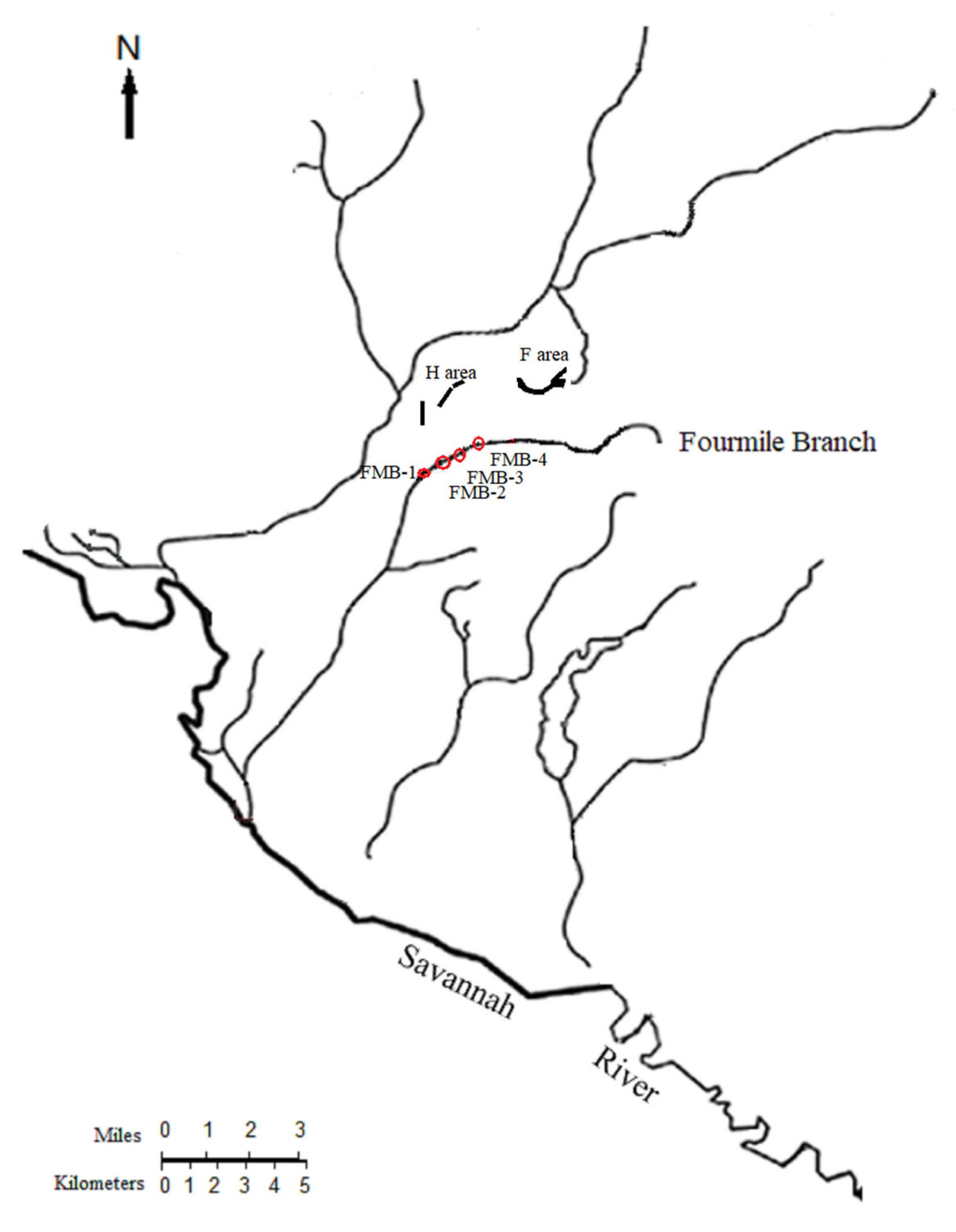
The watersheds of the Savannah River Site (SRS, Aiken, SC, USA) showed elevated Hg concentrations in the sediment and biota due to the legacy contamination from upstream industrial activities such as the Olin Corporation Chlor-Alkali Plant (Augusta, GA, USA), the historical agricultural runoff, and the SRS seepage basins that received liquid effluents containing Hg before the 1980s [23,47,48,49,50]. The Fourmile Branch (Figure 1) is a contaminated water body on the Savannah River Site; it received Hg release from multiple sources in different portions of the stream, with the two major sources having seeped through two basins—the F-area and H-area seepage basins [23,51,52]. As a third-order tributary of the Savannah River on the upper coastal plain of South Carolina, the FMB begins upstream from Road F, flows into the Savannah River through the Savannah River Swamp, and eventually becomes mixed with the Savannah River [53]. Since the Savannah River provides drinking water to the major metropolitan areas in Georgia (e.g., Augusta and Savannah) and South Carolina (Beaufort and Hilton Head), it is important to study the sources, environmental fate, and potential impacts of contaminants in the river and its tributaries, especially for contaminants of high concern such as Hg.

A previous study at the FMB explored Hg deposition and bioaccumulation near the H-area seepage basin [23]. To investigate the distribution of Hg in the FMB, this study focused on the other seepage basin: the F-area seepage basin. Four sampling sites were selected near the F-area seepage basin, based on Hg contamination levels, lithology, and plant root matter in the FMB [23,47]. The average water depth of the sampling sites was about 1 m. The sediments were mostly silt in the surface layer and sand in the medium and bottom layers for the four sites.

2.2. Sampling Strategy

Abiotic and biotic samples were taken from four sites at the FMB near the F-area seepage basin in the summers of 2017 and 2018 (Figure 1). Biotic samples, including biofilms, aquatic invertebrates, and fish, were first collected. Abiotic samples, including the bulk sediment and porewaters, were sampled after collecting biota to avoid the disturbance of the sediment and water systems. The porewaters were collected with a modified peeper device deployed in the sediment for 28 days, reaching a depth of approximately 28 cm below the SWI. At the end of the peeper deployment, bulk sediments were taken using traditional cores, and water quality parameters were measured at the SWI. A total of 4 sediment cores (with each core sectioned into 8 samples), 4 peepers (with each peeper containing 8 peeper vials), and 82 biotic samples were collected. All samples were properly processed and measured for total Hg and methyl-Hg concentrations. Details are included in Section 2.3, Section 2.4, Section 2.5 and Section 2.6.

2.3. Sediment Porewater

The sediment porewater was sampled using the peeper device designed by Pesch et al. [54], Serbst et al. [37], analyzed by Bufflap and Allen [55] and Brown and Caldwell [56], and modified by Qin et al. [57], as shown in Figure S1. One peeper device consisted of a polyvinyl chloride pipe (height: 102 cm; diameter: 8.9 cm) with 8 peeper vials (metal-free plastic vials; capacity: 50 mL; VWR International; Radnor, PA, USA) inserted at 4.0 cm intervals. The inserted peeper vials were constructed according to the designs described by Pesch et al. [54] and Serbst et al. [37]; a dialysis membrane disk (diameter: 4.9 cm; 0.45 µm; Biotrans; Brockton, MA, USA) was placed over the vial opening, and the original cap was perforated with several 0.5 cm holes. The peeper vials were assembled in a decontaminated and deoxygenated environment—a Milli-Q (Thermo Scientific; Waltham, MA, USA) water bath purged with nitrogen (oxygen < 0.5 mg/L). All vial components were washed with 5% nitric acid and rinsed before the assembly. The membrane disks, vials, caps, strings, and transport Ziploc bags were submerged in the water bath before the assembly. Deoxygenated water from the bath was used to fill each vial. The opening of the vial was covered with one membrane disk, secured with strings to keep the membrane in place, and closed with the perforated cap [57]. The assembled peeper vials were inspected to confirm that the edges of the membrane disks were secured and no air bubbles were retained. Each peeper vial was then placed into a submerged Ziploc bag, which was also filled with deoxygenated water from the bath and sealed while submerged. The Ziploc bags with the assembled peeper vials were preserved on ice in a cooler for transport to the field.

The peepers were installed onto the holding pipe in the field before deployment. One peeper pipe was deployed at each sampling site (FMB-1, FMB-2, FMB-3, and FMB-4; Figure 1). The peeper vials were taken out of the Ziploc bag and immediately inserted at the corresponding positions on the pipe. The assembled peeper pipe was then pushed into the sediment to the desired depth in the pre-determined sampling sites. The depth position of the pipe was determined by the upper two peeper vials; the second vial was kept just below the surface sediment, while the first vial was covered by the floc layer. According to our design and sampling protocol, each peeper pipe held 8 peeper vials at 4 cm intervals, with the top vial placed 4 cm above the SWI (0 cm), the second near the SWI (0 cm), and the other six at 4, 8, 12, 16, 20, and 24 cm below the SWI. In this study, the sampling depth above the SWI was presented as positive numbers and below as negative numbers. We did not deploy duplicate peeper pipes in each sampling site for two reasons: (1) after deploying one pipe, the sediment profiles nearby were extensively disturbed due to the difficulty of pushing the pipe into the hard sediment while keeping each vial in place on the pipe, so there would not be a real duplicate considering the disturbed status of the sediment; (2) we considered deploying duplicate pipes at the same distance to the F-Area seepage basin, but the sampling stream was too narrow to hold a duplicate pipe that was close enough to the first pipe to maintain the same distance to the seepage basin and far enough to avoid the sediment disturbance caused by deploying the first pipe.

The peeper pipes were retrieved after 28 days of deployment. The surface sediments around the pipe were carefully removed until the top four peeper vials were visible and the middle and bottom sediments were loosened. The pipe was then carefully pulled out of the sediment. Each peeper vial was checked for its position on the pipe and inspected for cap sealing. The particles outside the vial were rinsed with a gentle stream of Milli-Q water. The collected peeper vials were transported to the lab on ice. The membrane disk was carefully removed and inspected for integrity, color, biological growth, and precipitates. The peeper vial was then closed with an unperforated and cleaned (acid-washed and deoxygenated) cap. One peeper vial (FMB-1; −24 cm depth) was excluded from any future analysis because its membrane disk was damaged and there was dirt in the porewaters.

The porewater samples collected by each peeper vial were separated into several aliquots to analyze the THg, dissolved organic carbon (DOC), chloride, and sulfate concentrations. We did not measure the MHg concentrations in porewaters due to the unavoidable artifactual increase in MHg, as reported by Mason et al. [39]. The porewaters for the Hg measurements were preserved with acid, as described in Section 2.6, and for other measurements they were stored at 4 °C before the analysis.

2.4. Bulk Sediment

Manually deployed push tubes were used to collect sediment cores. Undisturbed sediment cores were taken before retrieving the peepers so that the sediment profile was not disturbed during the collection of porewaters. Each core was pushed to the same depth of the peeper pipe. One core was taken from each site near the sampling spot for the porewaters and at the same depth as the deployed peeper pipes. The reason for not taking duplicate sediment cores was the same as the reason for not deploying duplicate peeper pipes. The collected sediment cores were kept upright, put on ice, transferred to the lab, and stored at 4 °C for 4 to 8 h to let the flocculent precipitate.

The surface water on top of the flocculent layer and surface sediment was carefully siphoned off. The cores were then stored at −20 °C until frozen. Each sediment core was cut into 8 sections at 4 cm intervals, corresponding to the 8 peeper vials at the same depths. The organic matter above the SWI was the flocculent layer (depth: 4 cm), and the six sections below the SWI (depths: −4, −8, −12, −16, −20, and −24 cm) were the sediment layers. The cut and extruded sediment sections were then transferred to 50 mL metal-free tubes (VWR International; Radnor, PA, USA), freeze-dried (Labconco Corporation; Kansas City, MO, USA) until reaching a constant weight, and sieved with a mesh aperture of 2 mm before the Hg measurements.

2.5. Biota

The biotic samples were collected from the same sampling sites where the sediment cores and porewaters were taken (Figure 1). Un-baited traps, such as minnow traps and hoop nets, were used to catch fish and large aquatic invertebrates such as crustaceans and shrimps. The organisms were first identified after their capture in the field, then transported to the lab on ice and euthanized under the University of Georgia IACUC protocols (A2015 03-012-Y1-A1 and 12-009-Y3-A3). The wet weight and total length were determined for the fish and invertebrates. Eleven species were sampled: crayfish (Cambarus/Procambarus spp.), grass shrimp (Palaemonetes paludosus), dollar sunfish (Lepomis marginatus), spotted sunfish (Lepomis punctatus), bluespotted sunfish (Enneacanthus gloriosus), pirate perch (Aphredoderous sayanus), redfin pickerel (Esox americana), yellow bullhead (Ameiurus natalis), creek chubsucker (Erimyzon oblongus), dusky shiner (Notropis cummingsae), and coastal shiner (Notropis petersoni).

Biofilm was also collected from the four sampling sites with floating frames [23]. Eight frames were used in total, with two for each sampling site. Four polycarbonate sheets (30 × 30 cm) were secured to each frame. The floating frames were suspended in the water column (upper 35 cm) for a month. After the deployment, each polycarbonate sheet was placed in a plastic bag and transported to the lab on ice. Biofilm material was collected from each polycarbonate plate by scraping it into a 50 mL metal-free vial. Large debris (e.g., leaves and twigs) was removed from the biofilm materials. All biotic samples, including biofilm, invertebrates, and fish, were stored at −20 °C, freeze-dried, and homogenized before the analysis.

2.6. Chemical Analysis

The total Hg concentrations in the porewaters (µg/L), sediments (µg/kg, dry weight), and biotic samples (µg/kg, dry weight) were analyzed with the atomic absorption spectrophotometry by a Direct Mercury Analyzer-80 (Milestone; Shelton, CT, USA) at the University of Georgia’s Savannah River Ecology Lab (Aiken, SC, USA). The porewater samples were preserved with 12 N hydrochloride acid [58]. Calibration curves were built with DORM-3 (Fish protein; National Research Council of Canada; Ottawa, Canada) within each analytical session. The analytical precision and accuracy were quantified with blanks, replicated samples, matrix spike samples (spiked with a Hg standard from Sigma Aldrich; Rockville, MD, USA), and the certified standard reference material TORT-3 (Lobster hepatopancreas; National Research Council of Canada; Ottawa, ON, Canada). Each THg sample was measured three times and an average was calculated. The mean percent recovery of matrix spike samples was 98.6% (SD = 12.0%, n = 4) and of TORT-3 was 97.1% (SD = 6.0%, n = 12). The method precision, expressed as relative percent difference, averaged 3.4% (SD = 2.0%, n = 8) for the replicated aqueous samples and 5.4% (SD = 2.1%, n = 6) for the replicated solid samples. The method detection limits of THg were 0.06 ng and 0.03 ng for solid and aqueous samples, respectively.

The concentrations of MHg in the sediment (µg/kg, dry weight) and biotic samples (µg/kg, dry weight) were analyzed with a MERX Automated Methylmercury System (Brooks Rand; Seattle, WA, USA) at the University of Georgia’s Savannah River Ecology Lab (Aiken, SC). The sediment samples were prepared by acid leaching, solvent extraction, and water back-extraction [59]. The biotic samples were extracted with alkaline (25% (w/v) KOH in methanol) at 75 °C for 3 h [1]. Each MHg sample was measured three times and an average was calculated. Appropriate aliquots of water samples or diluted sediment extracts were then reacted with acetic acid and sodium tetraethylborate [60,61]. The reacted samples were introduced into gas chromatographic separation and pyrolysis and then measured using the cold vapor atomic fluorescence [1]. Calibration curves were built using the liquid CH₃HgCl (Brooks Rand; Seattle, WA, USA) within each analytical session. The analytical precision and accuracy were quantified with blanks, replicate samples, and the standard reference material TORT-3. The mean percent recovery of TORT-3 was 91.1% (SD = 7.0%, n = 12). The relative percent difference averaged 3.4% (SD = 2.5%, n = 6) for replicated solid samples. The method detection limits of MHg were 0.02 ng/g for solid samples.

Anions and organic matter in the porewaters were analyzed at the University of Georgia’s Center of Applied Isotope Studies (Athens, GA, USA). DOC concentrations were analyzed with a Total Carbon Analyzer-Model 500 (Shimadzu Inc; Durham, NC, USA) using high-temperature combustion. The mean percent recovery of the SPEX carbon standard (SPEX CertiPrep; Metuchen, NJ, USA) was 102.3% (SD = 0.12%, n = 3). Anion (sulfate and chloride) concentrations were measured with an ion chromatograph (Dionex; Sunnyvale, CA, USA). The mean percent recovery of the Dionex 7 Anion Standard II (Thermo Fisher Scientific; MA, USA) was 104.1% (SD = 1.5%, n = 2) for sulfate and 101.5% (SD = 3.9%, n = 2) for chloride. The relative percent differences for the replicated anion samples averaged 2.7% (SD = 3.8%, n = 4) for sulfate and 5.0% (SD = 7.1%, n = 4) for chloride.

The stable carbon and nitrogen isotopic signatures in the biotic samples were analyzed at the University of Georgia’s Center of Applied Isotope Studies (Athens, GA, USA). An aliquot of the freeze-dried and homogenized samples was weighed and packaged into a tin capsule. The isotopic ratios were determined with a PDZ Europa ANCA-GSL elemental analyzer interfaced with a PDZ Europa 20–20 isotope ratio mass spectrometer. Isotopic signatures were expressed as ratios (‰) normalized to the isotopic composition of Pee Dee Belemnite Limestone (δ¹³C) or atmospheric N₂ (δ¹⁵N) standards. The mean percent recoveries of 1577c (National Institute of Standards & Technology; Gaithersburg, MD, USA) were 100.0% (SD = 0.1%, n = 19) for carbon and 100.1% for nitrogen.

2.7. Statistics

The data were presented by the mean, standard deviation (SD), and sample size (n). SigmaPlot 13 (Systat 13; San Jose, CA, USA) was used for the general statistical analysis. We used multiple linear regression to explore variations in porewater Hg concentrations relative to the water quality chemistry, e.g., DOC, chloride, and sulfate. In this model, all variables were random effects, the interaction term was not involved, and all concentrations were log-transformed to meet the assumptions of normality and homogeneous variances across the levels of factors.

The mercury speciation in waters at the SWI was predicted with the Windermere Humic Aqueous Model 7 (WHAM 7; Lancaster, UK). Before the deployment and retrieval of the peepers, the water pH, temperature, and ORP (Oakton pH 6+ and ORPTestr 10; Vernon Hills, IL, USA) were measured twice in situ near the peeper pipes at the SWI (same depth as the second peeper vial). The measurement of water quality parameters followed the procedure described by Xu et al. [23]. The input variables of the speciation model included the water quality parameters measured in the field and the chemical concentrations (Hg, DOC, sulfate, and chloride) analyzed in the lab. The methyl-Hg concentrations in porewaters were derived from a previous study at the FMB [23]. Details of the model establishment were described by Xu and Mills [62].

The biomagnification model of MHg in the biotic samples was established with the relative trophic levels (TLs) estimated from stable carbon and nitrogen isotopic ratios. Assuming the biofilm trophic level is 1 [63] and the δ¹⁵N enriches 3.4‰ per trophic leve [64], the trophic level of the organism “i” can be calculated using Equation (1) based on its δ¹⁵N and the mean δ¹⁵N of biofilm [43]:

$$T{L}_i=1+\frac{{\delta }^{15}{N}_i-{\delta }^{15}{N}_{biofilm}}{3.4}$$

(1)

Linear regression was then fit to the log-transformed MHg concentrations for the collected biota using the relative TLs, as described in Equation (2):

$${\mathrm{Log}}_{10}\left[\mathrm{MHg}\right]=\mathrm{slope} \times \mathrm{TL}+\mathrm{intercept}$$

(2)

The food web magnification factor (FWMF) was eventually calculated using slopes in the linear regression, as shown in Equation (3):

$$\mathrm{FWMF}={10}^{\mathrm{slope}}$$

(3)

3. Results

3.1. Mercury in Bulk Sediment

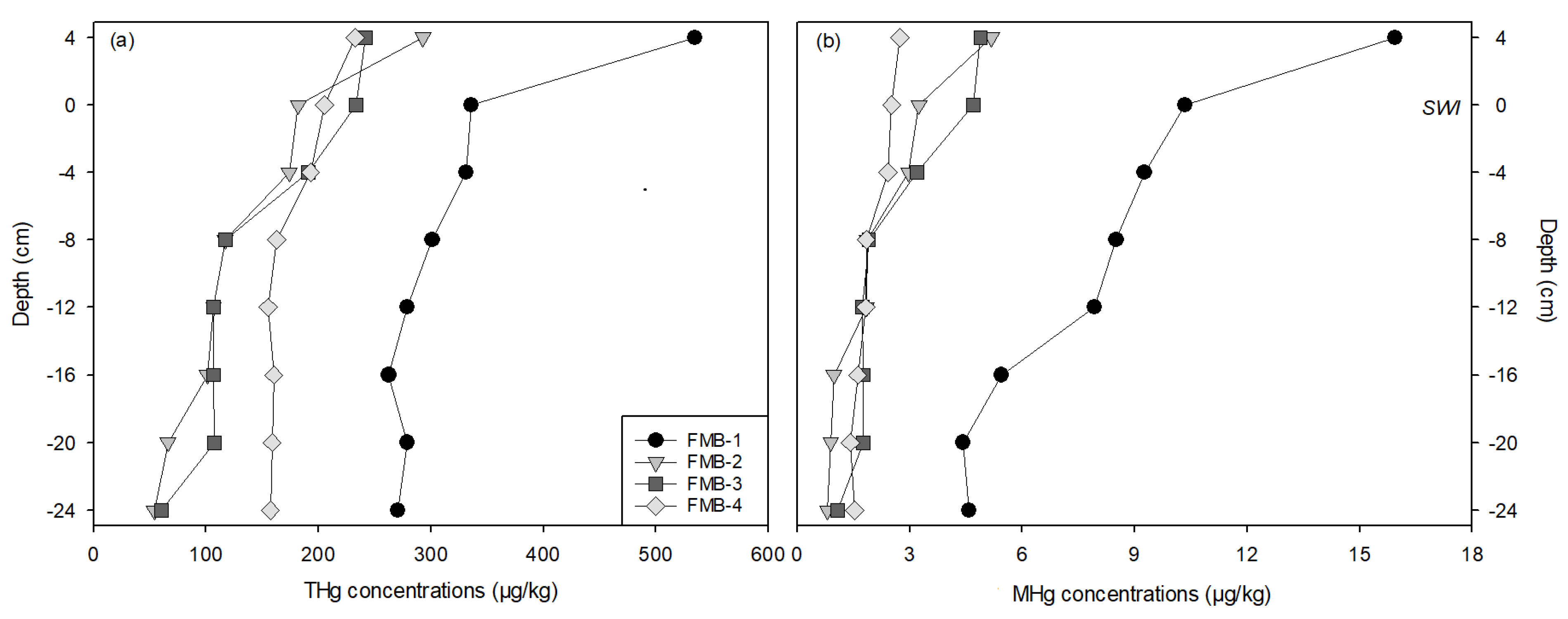
The depth profiles of Hg (THg and MHg) concentrations in bulk sediments are presented in Figure 2 and Table S2. The THg concentrations ranged from 53.8 to 534.3 µg/kg and the MHg concentrations from 0.8 to 15.9 µg/kg. Both the THg and MHg concentrations tended to decrease with increasing depth. The average concentrations of the upper three layers (4, 0, and −4 cm) were statistically higher than those of the other layers (p < 0.01) for all sites. FMB-1 presented the highest THg and MHg concentrations at each depth. The depth-averaged Hg concentrations were not statistically different among sites FMB-2, -3, and -4.

The %MHg at all depths and all sites was lower than 4% (0.9 to 3.1%). The mean %MHg in the lower three layers (−16, −20, and −24 cm) was statistically lower than those in the upper layers (p < 0.01). The highest and lowest depth-averaged %MHg was at FMB-1 and FMB-4, respectively.

3.2. Mercury in Sediment Porewaters

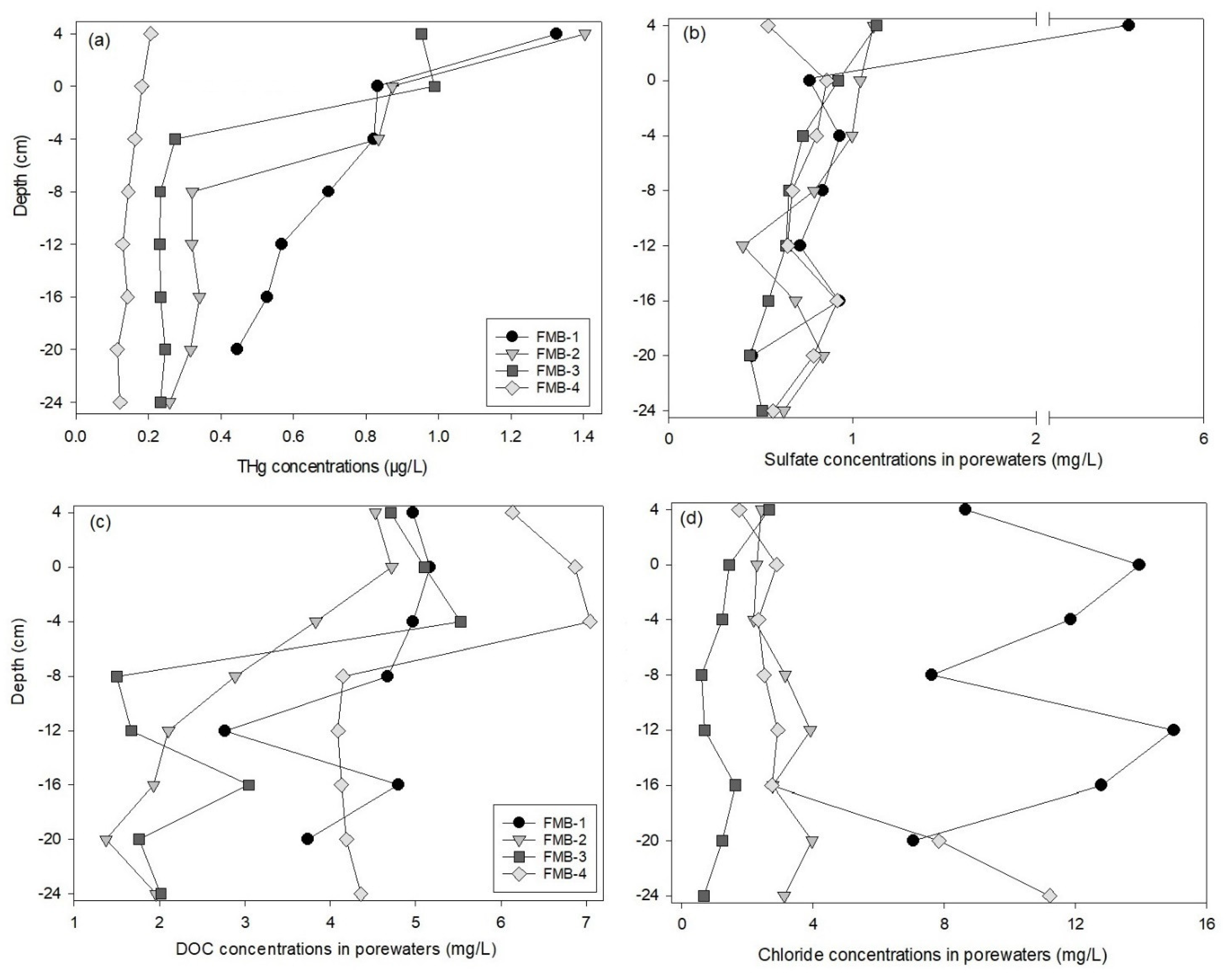
The depth profiles of Hg concentrations in the sediment porewaters are shown in Figure 3 and Table S3. The THg concentrations ranged from 0.11 to 1.40 µg/L. The layer (4 cm) above the SWI in FMB-2 indicated the highest THg concentrations among all sites and depths. The depth-averaged THg concentrations in FMB-4 (0.15 ± 0.03 µg/L) were statistically lower (p < 0.01) compared to the other sites. Sites FMB-1, -2, and -3 indicated obvious differences in Hg concentrations among depths; the THg concentrations tended to decrease with increasing depths and the average concentrations at and above the SWI (0 and 4 cm) were statistically higher than those below the SWI (p < 0.05). The THg concentrations of FMB-4, however, were relatively consistent among sampling depths.

Compared to the THg in the bulk sediments, the porewaters presented much lower concentrations at each depth for all sampling sites. The depth-averaged THg in the porewaters accounted for <0.5% of THg in the bulk sediment (FMB-1 = 0.2%, FMB-2 = 0.5%, FMB-3 = 0.3%, FMB-4 = 0.1%).

The depth profiles of the sulfate, chloride, and DOC concentrations in the sediment porewaters are presented in Figure 3 and Table S3. There were no statistical differences in the sulfate concentrations among the depths in all sites except for FMB-1, where the sulfate concentration above the SWI (4 cm) was about six times higher than those of other depths. The DOC concentrations in FMB-2, -3, and -4 near the SWI (4, 0, and −4 cm depths) were higher than those from other depths, but no differences were observed among the depths above and below the SWI in FMB-1. No trend was discovered for the vertical distributions of chloride concentrations. FMB-1 presented much higher chloride concentrations (averaged among depths: 10.6 ± 1.25 mg/L; p < 0.01) than the other sites (FMB-2: 2.91 ± 1.17 mg/L; FMB-3: 1.32 ± 1.42 mg/L; FMB-4: 3.47 ± 1.56 mg/L).

We used multiple linear regression to explore variations in the THg concentrations relative to the water quality chemistries (e.g., DOC, chloride, and sulfate) in the sediment porewaters (Table S4). Data from the four sampling sites were pooled in this model. Only the slope of Log₁₀^Sulfate (slope = 0.87, p = 0.005) was higher than zero, suggesting positive influences of sulfate on the THg accumulation in porewaters. It should be noted that the p value of the constant was also lower than 0.05 (slope = −0.37, p = 0.047), indicating that other variables not included in this model had negative influences on the porewater THg. Correspondingly, positive relationships between the THg and sulfate concentrations in the porewaters of FMB-1, -2, and -3 were observed (Figure S2).

3.3. Mercury Speciation

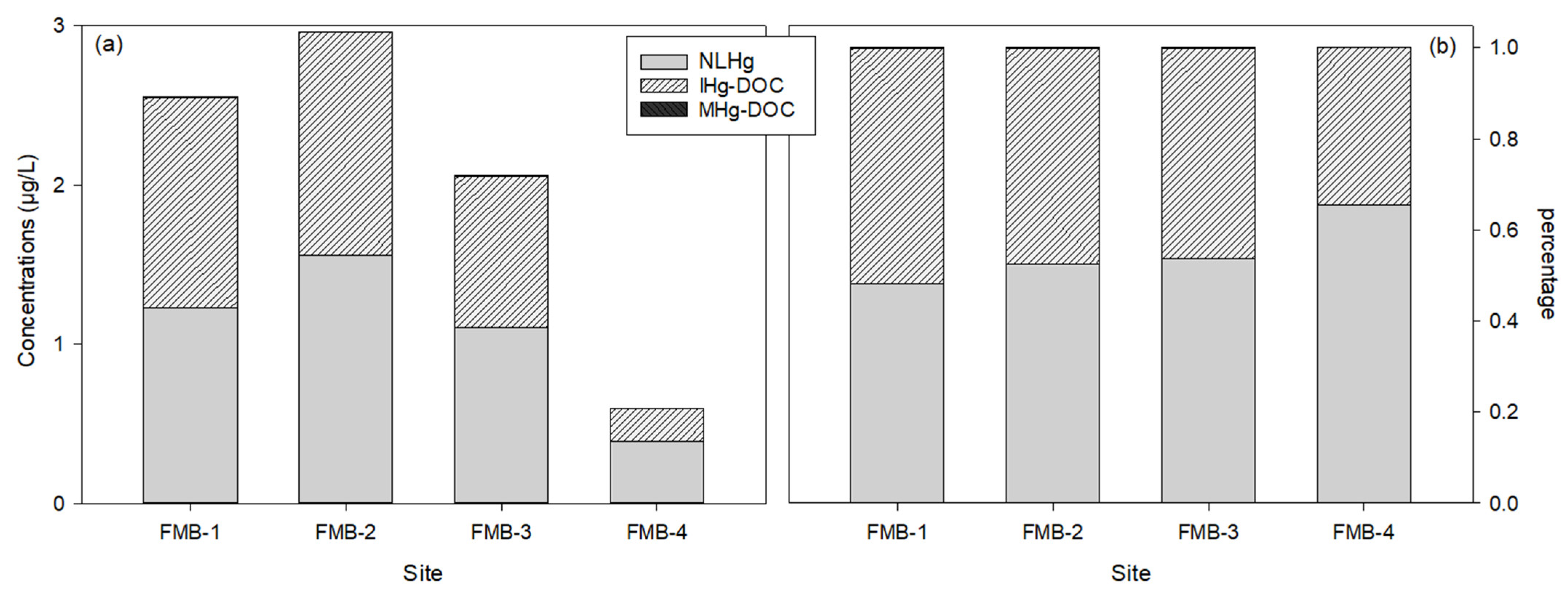
Figure 4 shows the Hg speciation at the SWI. The non-labile Hg (NLHg) concentrations were calculated by subtracting labile Hg from the THg (Table S1). Non-labile and labile Hg took an almost equal share of the THg; the site-averaged percentage of NLHg was 55.0%, and that of labile Hg was 45.0%. The labile Hg included inorganic Hg and methyl-Hg salts, and complexed inorganic Hg and methyl-Hg compounds. The dominant labile Hg species were DOC-complexed compounds, since IHg-DOC and MHg-DOC accounted for >99% of all the IHg and MHg species. The percentages of IHg and MHg salts were extremely low (<0.1%). When comparing the different speciation of IHg and MHg, IHg generally presented much higher concentrations in the DOC-complexed form (IHg-DOC: 0.97 µg/L) than MHg (MHg-DOC: 0.001 µg/L; p < 0.01). The IHg salts included Hg²⁺, HgOH⁺, Hg(OH)₂, Hg(OH)₃, and HgSO₄, and the MHg salts included CH₃Hg⁺ and CH₃HgOH. The concentrations of the IHg salts (5.2 × 10⁻²⁷ µg/L) were lower than the MHg salts (2.8 × 10⁻⁶ µg/L).

3.4. Mercury in Biota

The wet-weight-based THg concentrations in all the sampled fish were lower than the 300 µg/kg human health screening value [65]. The total Hg and methyl-Hg concentrations in the dry weight and %MHg in the biotic samples are shown in Figure S4 and Table S5. The %MHg in the THg of all fish ranged from 23 to 114%. The THg concentrations in the biofilms were relatively high, comparable to those in the dusky shiner, but the %MHg was the lowest among all biotic samples. There were no statistical differences in the THg or MHg concentrations for all fish species except for crayfish.

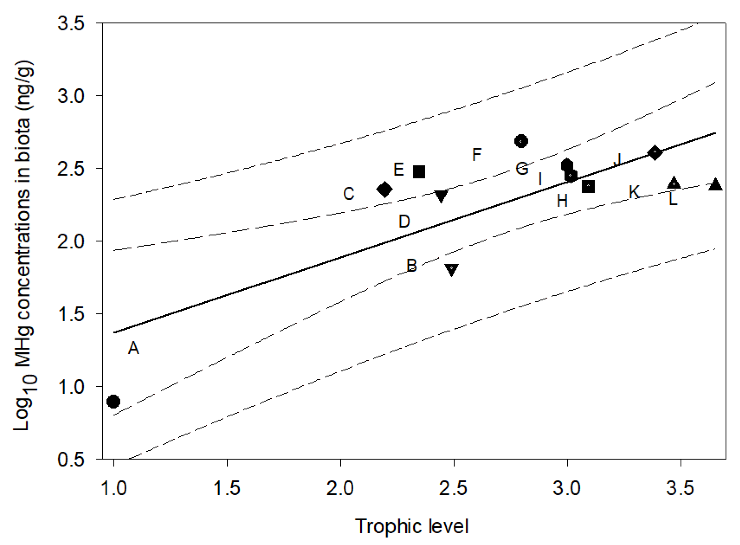
The MHg concentrations generally increased with δ¹⁵N values and trophic levels (Table S5). The biomagnification model for MHg was established for the collected biotic samples (Figure 5) using Equations (1) and (2):

$${\mathrm{Log}}_{10}\left[\mathrm{MHg}\right]=0.52\times \mathrm{TL}+0.84$$

(4)

where the p value of the slope was 0.003 and the adjusted r² was 0.55. The food web magnification factor was calculated using Equation (3):

$$\mathrm{FWMF}={10}^{0.52}=3.31$$

(5)

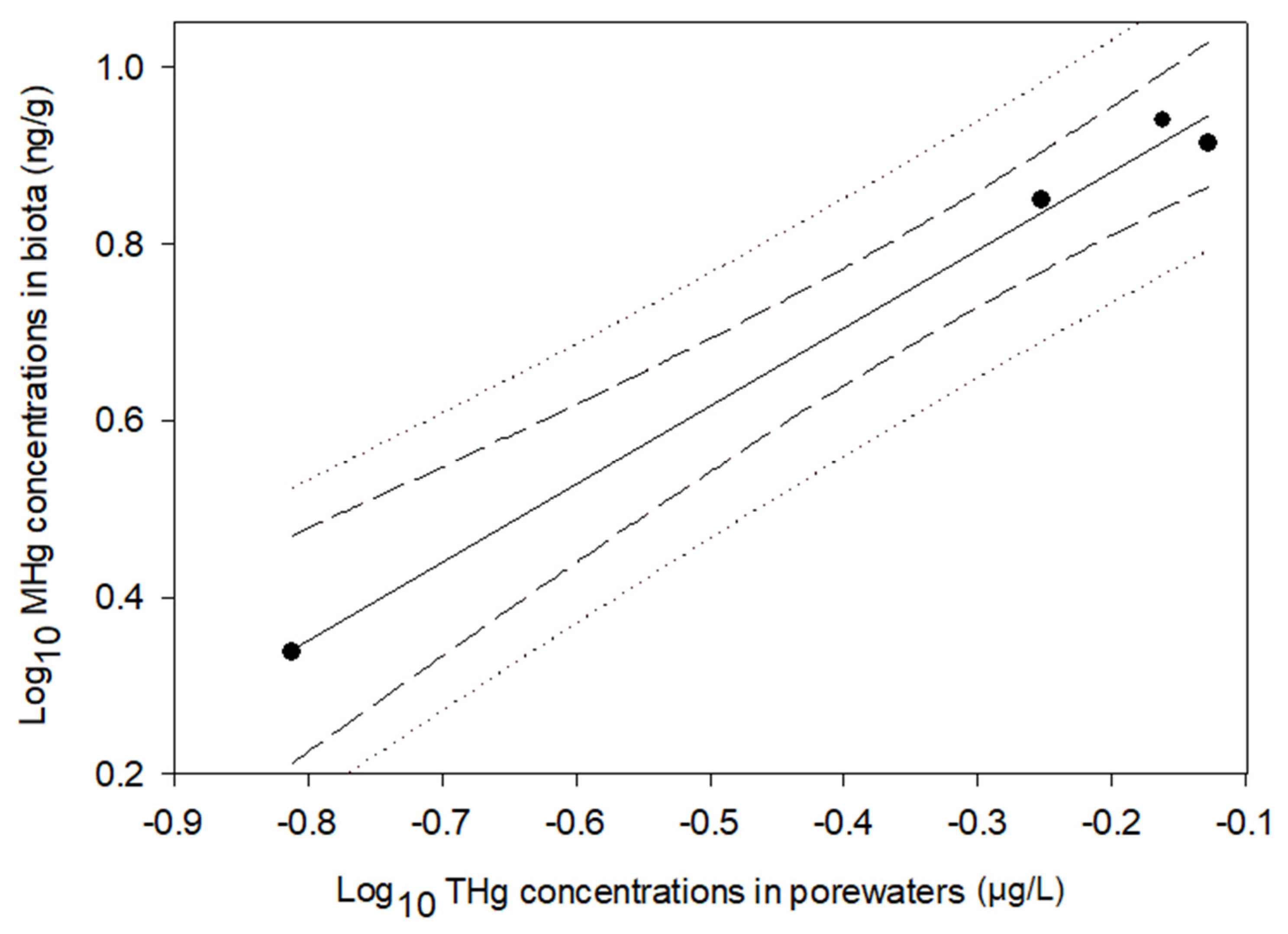
A positive relationship was observed between the THg concentrations in the sediment porewaters and the MHg concentrations in the biofilm (Figure 6):

Log₁₀[MHg_biofilm] = 0.91 Log₁₀[THg_porewater] − 1.13

(6)

where the p value of the slope was 0.006 and the adjusted r² was 0.98.

Therefore, the relationship between Hg in the biotic environment (biofilm) and Hg in the abiotic environment (sediment porewater) can be described as:

$$\left[{\mathrm{MHg}}_{\mathrm{biofilm}}\right]={10}^{\left(0.91\ast \log 10\left[\mathrm{THg} \mathrm{porewater}\right] – 1.13\right)}$$

(7)

4. Discussion

4.1. Mercury Deposition in the Sediment

Relatively high concentrations of total Hg (THg: 53.8 to 534.3 µg/kg) and methyl-Hg (MHg: 0.8 to 15.9 µg/kg, Figure 2) were observed in the sediment of the FMB. The vertical distributions of Hg in the bulk sediment and the porewaters presented consistent depositional features. The mercury concentrations in the top layers near the SWI (0 and 4 cm) were statistically higher than those of the bottom layers (p < 0.01), and the concentration decreased with increasing depths (Figure 2 and Figure 3). Previous studies have recorded similar vertical distributions. Sediment cores taken from the Pearl River Estuary (China) and Guanabara Bay (Brazil) both showed depositional profiles with the maximum Hg concentrations reaching from the surface to a depth of 10 cm below the surface [66,67]. Lambertsson and Nilsson [68] studied MHg in surface sediment of the Öre River Estuary (Sweden), where the MHg concentrations mostly varied in the upper 10 cm of sediments, peaking at depths between 0.5 and 2 cm.

The majority of deposited Hg in the sediment of the FMB was in the solid phase as non-labile species, because the Hg in the porewaters only made up <0.5% of the THg in the bulk sediment (Tables S2 and S3). As a soft B-group metal, Hg interacts weakly with oxygen-containing ligands, moderately with nitrogen-containing ligands, and strongly with sulfur-containing ligands. Among sulfur ligands, thiol-binding sites exhibit stronger interactions than oxidized sulfur sites [69]. The naturally occurring solid phase Hg, such as that in mine tailings, is usually associated with sulfur (α-HgS and β-HgS), oxygen (HgO), and chloride (HgCl₂). The importance of sulfide as a primary complexing agent for Hg has been pointed out by previous studies. Skyllberg [70] stated that, in an ecosystem without point sources, such as the current FMB, where the industrial release was ceased after the 1980s, sulfides are the only stable solid phases of IHg in the presence of natural organic matter (NOM). The role of NOM as a strong complexing agent for Hg has also been observed by many studies. The types of functional groups on the NOM determine the Hg speciation in the sediment. Mercury ions and salts tend to combine with the functional groups on NOM, especially the thiol groups, which determine the bonding of Hg to NOM pertaining to the solid and aqueous phases [10,22,71,72]. The Hg-NOM-thiol complexes in soils or sediment are usually formed as a two-coordinated linear complex with two thiol groups (Hg(SR)₂) in a stable bond, and with a third mono- or disulfide sulfur group in a weak bond if the Hg concentrations in the ambient environment are higher than 100 µg/g [73]. As the THg in the sediment of the FMB was lower than 100 µg/g, the major Hg-NOM-thiol complexes may form different coordinations (e.g., a one-coordinated linear complex). Furthermore, since the legacy Hg contamination in the FMB was mostly inorganic chloride salts released from industrial sources [48], the solid-phase Hg may also include HgCl₂-NOM and/or CH₃HgCl-NOM, although the NOM-complexed compounds are not as stable as the sulfur compounds.

The liquid-phase Hg in the sediment porewaters of the FMB (0.11 to 1.40 µg/L) was higher than reported data from other lakes (7.58 to 19.70 ng/L), estuaries (6.62 to 4.68 ng/L), and rivers (19 to 56 ng/L in the Toce River, Italy; 0.4 to 6.63 ng/L in the South River, VA, USA) [74,75,76,77]. We think the high THg levels in the porewaters might be related to reduced sulfur groups in the dissolved organic matter (DOM). Kneer et al. [78] conducted a similar study in the St. Louis River estuary sediments, where they found that the high THg concentrations in porewaters were related to high levels of reduced sulfur groups in the DOM, and the conditions facilitating greater partitioning of the THg to the porewaters were linked to sediments with low THg concentrations. Although reduced sulfur groups were not measured in the FMB, relatively high sulfate concentrations were observed in the porewaters. Thus, we assumed that the reduced sulfur in porewaters might have contribute to the high accumulations of liquid-phase Hg in the FMB sediment. Meanwhile, the THg concentrations in the bulk sediment of the FMB were not statistically different from Kneer et al.’s [78] results, also reflecting the conditions that sediments with low THg concentrations facilitate the partitioning of Hg to porewaters.

The primary Hg species in the porewaters of the FMB were DOC-complexed compounds. WHAM predicted a strong interaction between the THg and the DOC—that over 99% of the liquid-phase Hg was combined with DOC (Figure 4). The concentrations of the un-complexed Hg, the Hg salts, were extremely low (0.04 µg/L). The modeling output corresponds to previous experimental and modeling conclusions that the speciation of Hg compounds in aquatic systems is affected by the presence of inorganic (e.g., sulfide, chloride, and hydroxide) and/or organic (e.g., fulvic acid and humic acid) ligands, and that in freshwater systems, organic ligands likely dominate the chemistry of Hg species [23,79,80,81,82]. Similar to the speciation of solid-phase Hg, we think the complexes of the liquid-phase Hg in the porewaters were also combined with thiol functional groups on the DOC [72,83].

Complexity and diversity exist in the reactions between organic matter and Hg due to the various molecules comprising organic matter [84]. This study used the 0.45 µm dialysis to collect porewaters and arbitrarily defined the collected organic matter as dissolved versus particulate. Therefore, the collected DOM was likely a complex mixture of organic compounds that were either truly dissolved, aggregated into colloids, or associated with inorganic colloids or filterable particles [85,86].

4.2. Mercury Methylation and Methylmercury Production

The methylation of IHg determines the production and bioaccumulation of MHg in an ecosystem [8]. During microbial processes, the intracellular corrinoid-binding protein HgcA transfers one methyl group on MHg to IHg, and the ferredoxin HgcB reduces the cobalamin in HgcA for a new cycle of methylation [87,88]. It has been indicated that the cellular uptake of IHg by microorganisms and the biogeochemical factors that control the uptake are the factors that primarily determine the rate and amount of MHg production [11,12,89,90].

In aquatic systems, microbial methylation is subject to all geochemical perturbations related to methylation potentials and methylation reactions [10,24,25]. For instance, elevated sulfate concentrations could enhance sulfate reduction during in situ methylation, but the buildup of sulfide will instead limit the microbial processes [21]. Recent studies have found that the intermediate products generated from sulfate reduction and sulfide oxidation, such as thiosulfate and polysulfides, may increase the bioavailable Hg species within the water level fluctuation zone of a reservoir [18]. Organic matter is another major factor affecting the methylation capacity of an ecosystem. Generally, the chelation of IHg by organic matter tends to lower its bioavailability to methylators; however, this effect can be masked by stimulation microbes or the increased extent and duration of anoxic conditions in the water [19,20]. Additionally, the speciation of Hg, especially IHg as the major methylation potential, directly determines the bioavailability of Hg to microorganisms and thus influences microbial MHg production. Bioavailable IHg mostly does not exist on its own in anaerobic environments, but exists predominantly in forms that are complexed with NOM or sulfide particles, such as the weakly sorbed and amorphous IHg species, IHg-DOC complexes, and β-HgS nanoparticulate [10,22,23]. Mercury methylation also depends on the activity of the anaerobic microbiome that is capable of altering the environmental biogeochemistry, e.g., sulfide and organic matter, and subsequently alters the Hg speciation and bioavailability [22].

This study indicates positive influences of DOC and sulfate on the THg concentrations in porewaters (Table S4 and Figure 3). Sulfate is the essential stimulator for dissimilatory sulfate-reducing bacteria. DOC is the organic nutrient that provides energy for microbial activities. As two important methylation potentials, the combining conditions of DOC and sulfate enhanced the microbial methylation and MHg production in the FMB. Although the degradation of DOC may reduce Hg bioavailability and decrease methylation efficiency by forming complexes between IHg and inert organic matter (e.g., low-molecular weight and thiol-containing organic molecules) [91], we did not find any inhibiting effects of DOC. As the constant in the multiple linear regression indicated a significant negative influence on MHg variations (Table S4), other environmental factors such as the pH, alkalinity, and iron chemistry may have also influenced Hg methylation in the FMB sediment. Among these factors, iron is likely to have decreased MHg production by reducing the Hg bioavailability through chemical speciation [14,15].

Different sites presented different levels of Hg accumulation and methylation. Within the FMB, FMB-1 showed the highest Hg (THg and MHg) concentrations at all sampling depths in the bulk sediment, as well as the highest depth-averaged THg concentrations in the porewaters. We think the distance to the Hg source is the primary cause of the observed differences, because among the four sampling sites, FMB-1 was the closest to the F-area seep line (Figure 1). Meanwhile, the spatial heterogeneity of the river stretch may have also contributed to the observed differences. The above-mentioned reasons could also explain the higher sediment and porewater Hg concentrations observed by the present study in the F-area seepage basin, compared to those collected near the H-area seepage basin [23]. When compared to other aquatic systems, the %MHg in the THg of the sediments (0.9 to 3.1%, Table S2) of the FMB was generally higher than the estuarine sediments (<1%) [92], although Lambertsson and Nilsson [68] reported an expectedly high %MHg (4 to 13%) in the sediment of the Öre River estuary. The microbial activities and environmental factors related to methylation potentials and Hg speciation could have contributed to the differences among aquatic systems.

4.3. Mercury in Biotic and Abiotic Environments

Considering the disadvantages of biomonitoring in contamination monitoring, such as the expenses for collecting and processing procedures that pose limitations on sampling a normal population and excluding the influences of complicated biotic factors [93,94], alternative approaches such as passive samplers and geochemical speciation models have been adopted. This study applied WHAM to explore the speciation of labile Hg in sediment porewaters and collected labile Hg species with peepers. We aimed to link the Hg biomagnification to the labile Hg species in the sediment, so that Hg bioaccumulation at different trophic levels could be predicted through the data provided by passive samplers and modeling estimation.

First, the FWMF was calculated for the FMB. The MHg biomagnification model was established for the trophic web of the FMB (Figure 5) in this study, which stated that the MHg concentrations increased by 3.31 times per trophic level (FWMF = 3.31). This FWMF value was not statistically different from that derived from other portions of the FMB (4.4, 95%CI: 2.5–7.7) [23]. Therefore, the average of the two FWMFs was used here, which was 3.86. Secondly, a positive relationship between Hg in the biofilms and Hg in the porewaters was established (Figure 6, Equation (7)), indicating that the primary sources of bioaccumulative Hg originate from sediment porewaters. This positive correlation links Hg accumulation between abiotic (sediment) and biotic (biota) environments. For the future assessment of Hg in the tropic web of the FMB, it is possible to predict Hg bioaccumulation through Hg partitioning in porewaters: the Hg concentration in porewaters is transferred to biofilm first, and the Hg bioaccumulation of a certain trophic level can be calculated using the biofilm Hg and the FWMF (3.86) in Equation (5). This approach bypasses biota sampling as well as many other limitations associated with it, decreases the cost of contamination monitoring, and improves the efficiency of bioaccumulation assessment.

However, this approach will not apply to environments with continuous point sources where contaminants still deposit to the sediment. It also requires a thorough investigation of the Hg bioaccumulation in different seasons and sites of a target aquatic system, because the bioaccumulation pattern can vary with season or location. Although we did not observe differences in FWMF between two sampling locations in the FMB (near the F-area seepage basin and the H-area seepage basin) as discussed above [23], the Hg biomagnification could be variable in other sampling sites of the FMB. The FWMF in the winter season is also worth future studies, considering the seasonal changes in the parameters related to methylation, Hg speciation, and Hg bioavailability (e.g., DOC, sulfur, temperature, pH, ORP, etc.).

4.4. Application of Peepers

Contaminants in sediment porewater is always of great interest from a geochemical and toxicological perspective, as porewater is an important indicator of contaminant bioavailability and it mediates the fluxes between the sediment and the overlying water [95]. As one of the commonly applied passive samplers, the porewater diffusion equilibration sampler, or the so-called peeper, has been widely used to study the biogeochemistry of contaminants in the sediment for decades [37]. In the present study, we did not select the original peeper design, because a large area of its membrane was exposed to the ambient environment, making it vulnerable to the hard sediment of the FMB [30,96,97]. Our design, which stabilized the peeper vials on a holding pipe, was especially applied to solid sediment, but it could be used equally well in soft sediment and overlying water. It is worth noting that the depth interval on the peeper pipe, the numbers of attached peeper vials, and the deployment duration should be adjusted depending on specific research needs. Our results demonstrated the success of this peeper design in collecting small-scale structures of labile metals without disturbing the sediment profile, and it proved the feasibility of combining the geochemical model and the peeper for studying Hg speciation, methylation, and bioavailability in contaminated sediment.

5. Conclusions

This study investigated Hg deposition, speciation, methylation, and biomagnification in the abiotic and biotic environments of the FMB (SC < USA). Data were generated that corresponded to the four objectives of this study. (1) The majority of the Hg was deposited at the surface layers of the sediment, and the overall Hg concentrations in the bulk sediment (THg: 53.8 to 534.3 µg/kg; MHg: 0.8 to 15.9 µg/kg) and the porewater (THg: 0.11 to 1.40 µg/L) were high. The temporal and spatial variations of Hg deposition in the FMB were observed. (2) The sulfate level was the primary geochemical factor influencing Hg methylation and MHg production in the sediment. The dominant labile Hg species in the porewater was complexed with DOC, and concentrations of the IHg-DOC complexes (0.97 µg/L) were significantly higher than those of the MHg-DOC (0.001 µg/L). (3) MHg concentrations generally increased with trophic levels (biofilm < aquatic invertebrates < fish), and it increased by 3.31 times per trophic level. (4) As labile Hg concentrations in the porewaters were positively related to biofilm, a modified MHg magnification model was established to link the Hg in the abiotic environment (porewater) to the Hg bioaccumulation in the biotic environment (biota). In addition, our results also proved the feasibility of combining a geochemical model and a porewater sampler (peeper) for studying Hg speciation, methylation, and bioavailability in contaminated aquatic systems.

References

- Xu, X.; Zhang, Q.; Wang, W.-X. Linking mercury, carbon, and nitrogen stable isotopes in Tibetan biota: Implications for using mercury stable isotopes as source tracers. Sci. Rep. 2016, 6, 25394. [Google Scholar] [CrossRef] [PubMed] [Green Version]
- Branco, V.; Caito, S.; Farina, M.; daRocha, J.T.; Aschner, M.; Carvalho, C. Biomarkers of mercury toxicity: Past, present, and future trends. J. Toxicol. Environ. Health Part B Crit. Rev. 2017, 20, 119–154. [Google Scholar] [CrossRef] [PubMed]
- Newman, M.C.; Xu, X.; Condon, A.; Liang, L. Floodplain methylmercury biomagnification factor higher than that of the contiguous river (South River, Virginia USA). Environ. Pollut. 2011, 159, 2840–2844. [Google Scholar] [CrossRef] [PubMed]
- Jackson, T.A. Long-range atmospheric transport of mercury to ecosystems, and the importance of anthropogenic emissions—A critical review and evaluation of the published evidence. Environ. Rev. 1997, 5, 99–120. [Google Scholar] [CrossRef]
- Hudelson, K.E.; Drevnick, P.E.; Wang, F.; Armstrong, D.; Fisk, A.T. Mercury methylation and demethylation potentials in Arctic lake sediments. Chemosphere 2020, 248, 126001. [Google Scholar] [CrossRef]
- Liang, P.; Wu, S.; Zhang, C.; Xu, J.; Christie, P.; Zhang, J.; Cao, Y. The role of antibiotics in mercury methylation in marine sediments. J. Hazard Mater. 2018, 360, 1–5. [Google Scholar] [CrossRef]
- Ma, M.; Du, H.; Wang, D.; Kang, S.; Sun, T. Biotically mediated mercury methylation in the soils and sediments of Nam Co Lake, Tibetan Plateau. Environ. Pollut. 2017, 227, 243–251. [Google Scholar] [CrossRef]
- Compeau, G.; Bartha, R. Sulfate-reducing bacteria: Principal methylators of mercury in anoxic estuarine sediment. Appl. Environ. Microbiol. 1985, 50, 498–502. [Google Scholar] [CrossRef] [Green Version]
- Gerbig, C.; Kim, C.; Stegemeier, J.; Ryan, J.N.; Aiken, G.R. Formation of nanocolloidal metacinnabar in mercury-DOM-sulfide systems. Environ. Sci. Technol. 2011, 45, 9180–9187. [Google Scholar] [CrossRef]
- Deonarine, A.; Hsu-Kim, H. Precipitation of mercuric sulfide nanoparticles in NOM-containing water: Implications for the natural environment. Environ. Sci. Technol. 2009, 43, 2368–2373. [Google Scholar] [CrossRef]
- Wang, M.; Li, Y.; Zhao, D.; Zhuang, L.; Yang, G.; Gong, Y. Immobilization of mercury by iron sulfide nanoparticles alters mercury speciation and microbial methylation in contaminated groundwater. Chem. Eng. J. 2020, 381, 122664. [Google Scholar] [CrossRef]
- Gionfriddo, C.M.; Stott, M.B.; Power, J.F.; Ogorek, J.M.; Krabbenhoft, D.P.; Wick, R.; Holt, K.; Chen, L.; Thomas, B.C.; Banfield, J.F.; et al. Genome-resolved metagenomics and detailed geochemical speciation analyses yield new insights into microbial mercury cycling in geothermal springs. Appl. Environ. Microbiol. 2020, 86, e00176-20. [Google Scholar] [CrossRef] [PubMed]
- Liu, Y.; Whitman, W.B. Metabolic, phylogenetic, and ecological diversity of the methanogenic archaea. Ann. N. Y. Acad. Sci. 2008, 1125, 171–189. [Google Scholar] [CrossRef] [PubMed]
- Fleming, E.J.; Mack, E.E.; Green, P.G.; Nelson, D.C. Mercury methylation from unexpected sources: Molybdateinhibited freshwater sediments and an iron-reducing bacterium. Appl. Environ. Microbiol. 2006, 72, 457–464. [Google Scholar] [CrossRef] [Green Version]
- Kerin, E.J.; Gilmour, C.C.; Roden, E.; Suzuki, M.T.; Coates, J.D.; Mason, R.P. Mercury methylation by dissimilatory ironreducing bacteria. Appl. Environ. Microbiol. 2006, 72, 7919–7921. [Google Scholar] [CrossRef] [Green Version]
- Gilmour, C.C.; Podar, M.; Bullock, A.L.; Graham, A.M.; Brown, S.D.; Somenahally, A.C.; Johs, A.; Hurt, J.R.A.; Bailey, K.L.; Elias, D.A. Mercury methylation by novel microorganisms from new environments. Environ. Sci. Technol. 2013, 47, 11810–11820. [Google Scholar] [CrossRef]
- Yu, R.-O.; Reinfelder, J.R.; Hines, M.E.; Barkay, T. Mercury methylation by the methanogen Methanospirillum hungatei. Appl. Environ. Microbiol. 2013, 79, 6325–6330. [Google Scholar] [CrossRef] [Green Version]
- Liu, J.; Jiang, T.; Wang, F.; Zhang, J.; Wang, D.; Huang, R.; Yin, D.; Liu, Z.; Wang, J. Inorganic sulfur and mercury speciation in the water level fluctuation zone of the Three Gorges Reservoir, China: The role of inorganic reduced sulfur on mercury methylation. Environ. Pollut. 2018, 237, 1112–1123. [Google Scholar] [CrossRef]
- Mason, R.P.; Sheu, G.R. The role of the ocean in the global mercury cycle. Glob. Biogeochem. Cycles 2002, 16, 1093. [Google Scholar] [CrossRef]
- Schuster, P.F.; Shanley, J.B.; Marvin-Dipasquale, M.; Reddy, M.M.; Aiken, G.R.; Roth, D.A.; Taylor, H.E.; Krabbenhoft, D.P.; DeWild, J.F. Mercury and organic carbon dynamics during runoff episodes from a northeastern USA watershed. Water Air Soil 2008, 187, 89–108. [Google Scholar] [CrossRef] [Green Version]
- Benoit, J.M.; Gilmour, C.C.; Mason, R.P.; Heyes, A. Sulfide controls on mercury speciation and bioavailability to methylating bacteria in sediment pore waters. Environ. Sci. Technol. 1999, 33, 951–957. [Google Scholar] [CrossRef]
- Hsu-Kim, H.; Eckley, C.S.; Acha, D.; Feng, X.; Gilmour, C.C.; Jonsson, S.; Mitchell, C.P.J. Challenges and opportunities for managing aquatic mercury pollution in altered landscapes. Ambio 2018, 47, 141–169. [Google Scholar] [CrossRef] [PubMed] [Green Version]
- Xu, X.; Bryan, A.L.; Mills, G.L.; Korotasz, A.M. Mercury speciation, bioavailability, and biomagnification in contaminated streams on the Savannah River Site (SC, USA). Sci. Total Environ. 2019, 668, 261–270. [Google Scholar] [CrossRef] [PubMed]
- Obrist, D.; Kirk, J.L.; Zhang, L.; Sunderland, E.M.; Jiskra, M.; Selin, N.E. A review of global environmentalmercury processes in response to human and natural perturbations: Changes of emissions, climate, and land use. Ambio 2018, 47, 116–140. [Google Scholar] [CrossRef] [Green Version]
- Tang, W.-L.; Liu, Y.-R.; Guan, W.-Y.; Zhang, H.; Qu, X.-M.; Zhang, T. Understanding mercury methylation in the changing environment: Recent advances in assessing microbial methylators and mercury bioavailability. Sci. Total Environ. 2020, 714, 136827. [Google Scholar] [CrossRef]
- Rivera, N.A.; Bippus, P.M.; Hsu-Kim, H. Relative reactivity and bioavailability of mercury sorbed to or coprecipitated with aged iron sulfides. Environ. Sci. Technol. 2019, 53, 7391–7399. [Google Scholar] [CrossRef]
- Jiskra, M.; Saile, D.; Wiederhold, J.G.; Bourdon, B.; Bjorn, E.; Kretzschmar, R. Kinetics of Hg(II) exchange between organic ligands, goethite, and natural organic matter studied with an enriched stable isotope approach. Environ. Sci. Technol. 2014, 48, 13207–13217. [Google Scholar] [CrossRef] [Green Version]
- Stenzler, B.; Hinz, A.; Ruuskanen, M.; Poulain, A.J. Ionic strength differentially affects the bioavailability of neutral and negatively charged inorganic Hg complexes. Environ. Sci. Technol. 2017, 51, 9653–9662. [Google Scholar] [CrossRef]
- Ndu, U.; Christensen, G.A.; Rivera, N.A.; Gionfriddo, C.M.; Deshusses, M.A.; Elias, D.A.; Hsu-Kim, H. Quantification of mercury bioavailability for methylation using diffusive gradient in thin-film samplers. Environ. Sci. Technol. 2018, 52, 8521–8529. [Google Scholar] [CrossRef]
- Hesslein, R.H. An in situ sampler for close interval pore water studies. Limnol. Oceanogr. 1976, 21, 912–914. [Google Scholar] [CrossRef]
- Davison, W.; Grime, G.W.; Morgan, J.A.W.; Clarke, K. Distribution of dissolved iron in sediment pore waters at submillimeter resolution. Nature 1991, 352, 323–325. [Google Scholar] [CrossRef]
- Clarisse, O.; Foucher, D.; Hintelmann, H. Methylmercury speciation in the dissolved phase of a stratified lake using the diffusive gradient in thin film technique. Environ. Pollut. 2009, 157, 987–993. [Google Scholar] [CrossRef] [PubMed]
- Clarisse, O.; Dimock, B.; Hintelmann, H.; Best, E.P. Predicting net mercury methylation in sediments using diffusive gradient in thin films measurements. Environ. Sci. Technol. 2011, 45, 1506–1512. [Google Scholar] [CrossRef] [PubMed]
- Zhang, H.; Davison, W. Performance characteristics of diffusion gradients in thin films for the in situ measurement of trace metals in aqueous solution. Anal. Chem. 1995, 67, 3391–3400. [Google Scholar] [CrossRef]
- Philipps, R.R.; Xu, X.Y.; Bringolf, R.B.; Mills, G.L. Evaluation of the DGT technique for predicting uptake of metal mixtures by fathead minnow (Pimephales promelas) and yellow lampmussel (Lampsilis cariosa). Environ. Toxicol. Chem. 2019, 38, 61–70. [Google Scholar] [CrossRef] [Green Version]
- Philipps, R.R.; Xu, X.Y.; Mills, G.L.; Bringolf, R.B. Evaluation of diffusive gradients in thin films for prediction of copper bioaccumulation by yellow lampmussel (Lampsilis cariosa) and fathead minnow (Pimephales promelas). Environ. Toxicol. Chem. 2018, 37, 1535–1544. [Google Scholar] [CrossRef]
- Serbst, J.R.; Burgess, R.M.; Kuhn, A.; Edwards, P.A.; Cantwell, M.G.; Pelletier, M.C.; Berry, W.J. Precision of dialysis (peeper) sampling of cadmium in marine sediment interstitial water. Arch. Environ. Contam. Toxicol. 2003, 45, 297–305. [Google Scholar] [CrossRef]
- Liu, J.L.; Feng, X.B.; Qiu, G.L.; Yao, H.; Shang, L.H.; Yan, H.Y. Intercomparison and Applicability of Some Dynamic and Equilibrium Approaches to Determine Methylated Mercury Species in Pore Water. Environ. Toxicol. Chem. 2011, 30, 1739–1744. [Google Scholar] [CrossRef]
- Mason, R.; Bloom, N.; Cappellino, S.; Gill, G.; Benoit, J.; Dobbs, C. Investigation of porewater sampling methods for mercury and methylmercury. Environ. Sci. Technol. 1998, 32, 4031–4040. [Google Scholar] [CrossRef]
- Montgomery, S.; Mucci, A.; Lucotte, M. The application of in situ dialysis samplers for close interval investigations of total dissolved mercury in interstitial waters. Water Air Soil Poll. 1996, 87, 219–229. [Google Scholar] [CrossRef]
- Wang, J.; Newman, M.C.; Xiaoyu, X.; Condon, A.; Liang, L. Floodplain methylmercury biomagnification factor higher and more variable than that of the contiguous South River (Virginia USA). Ecotoxicol. Environ. Saf. 2013, 92, 191–198. [Google Scholar] [CrossRef] [PubMed]
- Mason, R.P.; Reinfelder, J.R.; Morel, F.M.M. Uptake, toxicity and trophic transfer of mercury in a coastal diatom. Environ. Sci. Technol. 1996, 30, 1835–1845. [Google Scholar] [CrossRef]
- Xu, X.; Newman, M.C.; Fabrizio, M.C.; Liang, L. An ecologically framed mercury survey of finfish of the lower Chesapeake Bay. Arch. Environ. Contam. Toxicol. 2013, 65, 510–520. [Google Scholar] [CrossRef] [PubMed]
- Watras, C.J.; Bloom, N.S. Mercury and Methylmercury in Individual Zooplankton—Implications for Bioaccumulation. Limnol. Oceanogr. 1992, 37, 1313–1318. [Google Scholar] [CrossRef]
- Bishop, C.A.; Koster, M.D.; Chek, A.A.; Hussell, D.J.T.; Jock, K. Chlorinated Hydrocarbons and Mercury in Sediments, Red-Winged Blackbirds (Agelaius-Phoeniceus) and Tree Swallows (Tachycineta Bicolor) from Wetlands in the Great-Lakes St-Lawrence-River Basin. Environ. Toxicol. Chem. 1995, 14, 491–501. [Google Scholar] [CrossRef]
- Horton, J.H. Mercury in the Separations Areas Seepage Basins; DPST-74-231; Du Pont: Aiken, SC, USA, 1997. [Google Scholar]
- Kuhne, W.W.; Halverson, N.V.; Jackson, D.G.; Jannik, G.T.; Looney, B.B.; Paller, M.H. 2015 Assessment of Mercury in the savannah River Site Environment and Responses to the Agency for Toxic Substances and Disease Registry 2012: Report on Assessment of Biota Exposure to Mercury Originating from the Savannah River Site; Savannah River Nuclear Solutions: Aiken, SC, USA, 2015. [Google Scholar]
- Smith, L.; Jagoe, C.; Carl, F. Chlor-alkali plant contributes to mercury contamination in the Savannah River. In Proceedings of the 2007 Georgia Water Resources Conference at the University of Georgia, Athens, GA, USA, 27–29 March 2007. [Google Scholar]
- Newman, M.C. Comprehensive cooling water report—Volume 2: Water quality. Natl. Tech. Inf. Serv. 1986, 2, 13–19. [Google Scholar]
- Haskins, D.; Brown, M.K.; Qin, C.; Xu, X.; Pilgrim, M.; Tuberville, T.D. Multi-decadal trends in mercury and methylmercury concentrations in the brown watersnake (Nerodia taxispilota). Environ. Pollut. 2021, 276, 116722. [Google Scholar] [CrossRef]
- Killian, T.H.; Colb, N.L.; Corbo, P.; Marine, I.W. Environmental Information Document F-Area Seepage Basin; Savannah River Lab: Aiken, SC, USA, 1987. [Google Scholar]
- Killian, T.H.; Colb, N.L.; Corbo, P.; Marine, I.W. Environmental Information Document H-Area Seepage Basin; Savannah River Lab: Aiken, SC, USA, 1987. [Google Scholar]
- Lanier, T.H. Determination of the 100-Year Flood Plain on Fourmile Branch at the Savannah River Site, South Carolina, 1996; Water-Resources Investigations Report 96-4271; U.S. Geological Survey: Columbia, SC, USA, 1997. [Google Scholar]
- Pesch, C.E.; Hansen, D.J.; Boothman, W.S.; Berry, W.J.; Mahony, J.D. The Role of Acid Volatile Sulfide and Interstitial Water Metal Concentrations in Determining Bioavailability of Cadmium and Nickel from Contaminated Sediments to the Marine Polychaete Neanthes Arenaceodentata. Environ. Toxicol. Chem. 1995, 14, 129–141. [Google Scholar] [CrossRef]
- Bufflap, S.E.; Allen, H.E. Comparison of pore-water sampling techniques for trace-metals. Water Res. 1995, 29, 2051–2054. [Google Scholar] [CrossRef]
- Brown, K.; Caldwell, D. Sampling Pore Water Sediments; Brown and Caldwell: Andover, MA, USA; Upper Saddle River, NJ, USA, 2016. [Google Scholar]
- Qin, C.; Xu, X.; Peck, E. Sink or source? Insights into the behavior of copper and zinc in the sediment porewater of a constructed wetland by peepers. Sci. Total Environ. 2022, 821, 153127. [Google Scholar] [CrossRef]
- USEPA. Method 1631, Revision E: Mercury in Water by Oxidation, Purge and Trap, and Cold Vapor Atomic Fluorescence Spectrometry; United States Environmental Protection Agency, Office of Water: Washington, DC, USA, 2002. [Google Scholar]
- Liang, L.; Horvat, M.; Feng, X.; Shang, L.; Li, H.; Pang, P. Re-evaluation of distillation and comparison with HNO3 leaching/solvent extraction for isolation of methylmercury compounds from sediment/soil samples. Appl. Organometal. Chem. 2004, 18, 264–270. [Google Scholar] [CrossRef]
- Liang, L.; Bloom, N.S.; Horvat, M. Simultaneous determination of mercury speciation in biological materials by GC/CVAFS after ethylation and room temperature precollection. Clin. Chem. 1994, 40, 602–607. [Google Scholar] [CrossRef] [PubMed]
- Liang, L.; Horvat, M.; Bloom, N.S. An improved speciation method for mercury by GC/CVAFS after aqueous phase ethylation and room temperature precollection. Talanta 1994, 41, 371–379. [Google Scholar] [CrossRef]
- Xu, X.; Mills, G.L. Do constructed wetlands remove metals or increase metal bioavailability? J. Environ. Manag. 2018, 218, 245–255. [Google Scholar] [CrossRef]
- Baird, D.; Ulanowicz, R.E. The seasonal dynamics of the Chesapeake Bay ecosystem. Ecol. Monogr. 1989, 59, 329–364. [Google Scholar] [CrossRef]
- Minagawa, M.; Wada, E. Stepwise enrichment of 15 N along food chains: Further evidence and the relation between 15 N and animal age. Geochim. Cosmochim. Acta 1984, 48, 1135–1140. [Google Scholar] [CrossRef]
- USEPA. EPA Releases Report on Fish Contamination in US Lakes and Reservoirs; United States Environmental Protection Agency, Office of Water: Washington, DC, USA, 2009. [Google Scholar]
- Shi, J.B.; Ip, C.C.M.; Zhang, G.; Jiang, G.B.; Li, X.D. Mercury profiles in sediments of the Pearl River Estuary and the surrounding coastal area of South China. Environ. Pollut. 2010, 158, 1974–1979. [Google Scholar] [CrossRef] [Green Version]
- Wasserman, J.C.; Freitas-Pinto, A.A.P.; Amouroux, D. Mercury concentrations in sediment profiles of a degraded tropical coastal environment. Environ. Technol. 2000, 21, 297–305. [Google Scholar] [CrossRef]
- Lambertsson, L.; Nilsson, M. Organic material: The primary control on mercury methylation and ambient methyl mercury concentrations in estuarine sediments. Environ. Sci. Technol. 2006, 40, 1822–1829. [Google Scholar] [CrossRef]
- Vairavamurthy, M.A.; Maletic, D.; Wang, S.K.; Manowitz, B.; Eglinton, T.; Lyons, T. Characterization of sulfur-containing functional groups in sedimentary humic substances by X-ray absorption near-edge structure spectroscopy. Energy Fuels 1997, 11, 546–553. [Google Scholar] [CrossRef]
- Skyllberg, U. Chemical speciation of mercury in soil and sediment. In Environmental Chemistry and Toxicology of Hg; Liu, G., Cai, Y., O’Driscoll, N., Eds.; John Wiley & Sons, Inc.: Hoboken, NJ, USA, 2012. [Google Scholar]
- Karlsson, T.; Skyllberg, U. Bonding of ppb levels of methyl mercury to reduced sulfur groups in soil organic matter. Environ. Sci. Technol. 2003, 37, 4912–4918. [Google Scholar] [CrossRef] [PubMed]
- Black, F.J.; Bruland, K.W.; Flegal, A.R. Competing ligand exchange-solid phase extraction method for the determination of the complexation of dissolved inorganic mercury(II) in natural waters. Anal. Chim. Acta 2007, 598, 318–333. [Google Scholar] [CrossRef] [PubMed]
- Skyllberg, U.; Bloom, P.R.; Qian, J.; Lin, C.M.; Bleam, W.F. Complexation of mercury(II) in soil organic matter: EXAFS evidence for linear two-coordination with reduced sulfur groups. Environ. Sci. Technol. 2006, 40, 4174–4180. [Google Scholar] [CrossRef] [PubMed]
- He, T.R.; Lu, J.; Yang, F.; Feng, X.B. Horizontal and vertical variability of mercury species in pore water and sediments in small lakes in Ontario. Sci. Total Environ. 2007, 386, 53–64. [Google Scholar] [CrossRef]
- Matsuyama, A.; Yano, S.; Taninaka, T.; Kindaichi, M.; Sonoda, I.; Tada, A.; Akagi, H. Chemical characteristics of dissolved mercury in the pore water of Minamata Bay sediments. Mar. Pollut. Bull. 2018, 129, 503–511. [Google Scholar] [CrossRef]
- Pisanello, F.; Marziali, L.; Rosignoli, F.; Poma, G.; Roscioli, C.; Pozzoni, F.; Guzzella, L. In situ bioavailability of DDT and Hg in sediments of the Toce River (Lake Maggiore basin, Northern Italy): Accumulation in benthic invertebrates and passive samplers. Environ. Sci. Pollut. Res. 2016, 23, 10542–10555. [Google Scholar] [CrossRef]
- Washburn, S.J.; Blum, J.D.; Kurz, A.Y.; Pizzuto, J.E. Spatial and temporal variation in the isotopic composition of mercury in the South River, VA. Chem. Geol. 2018, 494, 96–108. [Google Scholar] [CrossRef]
- Kneer, M.L.; White, A.; Rolfhus, K.R.; Jeremiason, J.D.; Johnson, N.W.; Ginder-Vogel, M. Impact of Dissolved Organic Matter on Porewater Hg and MeHg Concentrations in St. Louis River Estuary Sediments. ACS Earth Space Chem. 2020, 4, 1386–1397. [Google Scholar] [CrossRef]
- Liu, G.; Li, Y.; Cai, Y. Adsorption of mercury on soils in the aquatic environment. In Environmental Chemistry and Toxicology of Hg; Liu, G., Cai, Y., O’Driscoll, N., Eds.; John Wiley & Sons, Inc.: Hoboken, NJ, USA, 2012. [Google Scholar]
- Zhong, H.; Wang, W.X. Inorganic Mercury Binding with Different Sulfur Species in Anoxic Sediments and Their Gut Juice Extractions. Environ. Toxicol. Chem. 2009, 28, 1851–1857. [Google Scholar] [CrossRef] [Green Version]
- Fitzgerald, W.F.; Lamborg, C.H.; Hammerschmidt, C.R. Marine biogeochemical cycling of mercury. Chem. Rev. 2007, 107, 641–662. [Google Scholar] [CrossRef]
- Skyllberg, U.; Qian, J.; Frech, A. Combined XANES and EXAFS study on the bonding of methyl mercury to thiol groups in soil and aquatic organic matter. Phys. Scripta 2005, T115, 894–896. [Google Scholar] [CrossRef]
- Khwaja, A.R.; Bloom, P.R.; Brezonik, P.L. Binding strength of methylmercury to aquatic NOM. Environ. Sci. Technol. 2010, 44, 6151–6156. [Google Scholar] [CrossRef]
- Aiken, G.; Cotsaris, E. Soil and hydrology—Their effect on NOM. J. Am. Water Work. Assoc. 1995, 87, 36–45. [Google Scholar] [CrossRef]
- Pettit, R.E. Organic Matter, Humus, Humate, Humic Acid, Fulvic Acid and Humin: Their Importance in Soil Fertility and Plant Health. Available online: http://www.humates.com/pdf/ORGANICMATTERPettit.pdf (accessed on 1 May 2022).
- Gerbig, C.; Ryan, J.N.; Aiken, G.R. The effects of dissolved organic matter on mercury biogeochemistry. In Environmental Chemistry and Toxicology of Hg; Liu, G., Cai, Y., O’Driscoll, N., Eds.; John Wiley & Sons, Inc.: Hoboken, NJ, USA, 2012. [Google Scholar]
- Parks, J.M.; Johs, A.; Podar, M.; Bridou, R.; Hurt, R.A.; Smith, S.D.; Tomanicek, S.J.; Qian, Y.; Brown, S.D.; Brandt, C.C.; et al. The genetic basis for bacterial mercury methylation. Science 2013, 339, 1332–1335. [Google Scholar] [CrossRef] [Green Version]
- Zhou, J.; Riccardi, D.; Beste, A.; Smith, J.C.; Parks, J.M. Mercury Methylation by HgcA: Theory Supports Carbanion Transfer to Hg(II). Inorg. Chem. 2014, 53, 772–777. [Google Scholar] [CrossRef]
- Schaefer, J.K.; Rocks, S.S.; Zheng, W.; Liang, L.; Gu, B.; Morel, F.M.M. Active transport, substrate specificity, and methylation of Hg(II) in anaerobic bacteria. Proc. Natl. Acad. Sci. USA 2011, 108, 8714–8719. [Google Scholar] [CrossRef] [Green Version]
- Adediran, G.A.; Van, L.N.; Song, Y.; Schaefer, J.K.; Skyllberg, U.; Bjorn, E. Microbial biosynthesis of thiol compounds: Implications for speciation, cellular uptake, and methylation of Hg(II). Environ. Sci. Technol. 2019, 53, 8187–8196. [Google Scholar] [CrossRef]
- Barkay, T.; Gillman, M.; Turner, R.R. Effects of dissolved organic carbon and salinity on bioavailability of mercury. Appl. Environ. Microbiol. 1997, 63, 4267–4271. [Google Scholar] [CrossRef] [Green Version]
- Hines, M.E.; Horvat, M.; Faganeli, J.; Bonzongo, J.C.J.; Barkay, T.; Major, E.B.; Scott, K.J.; Bailey, E.A.; Warwick, J.J.; Lyons, W.B. Mercury biogeochemistry in the Idrija River, Slovenia, from above the mine into the Gulf of Trieste. Environ. Res. 2000, 83, 129–139. [Google Scholar] [CrossRef]
- Zhou, Q.; Zhang, J.; Fu, J.; Shi, J.; Jiang, G. Biomonitoring: An appealing tool for assessment of metal pollution in the aquatic ecosystem. Anal. Chim. Acta 2008, 606, 135–150. [Google Scholar] [CrossRef]
- Xu, X.; Peck, E.; Fletcher, D.E.; Korotasz, A.; Perry, J. Limitations of applying diffusive gradients in thin films to predict bioavailability of metal mixtures in aquatic systems with unstable water chemistries. Environ. Toxicol. Chem. 2020, 39, 2485–2495. [Google Scholar] [CrossRef]
- Teasdale, P.R.; Batley, G.E.; Apte, S.C.; Webster, I.T. Pore-water sampling with sediment peepers. Trac-Trend Anal. Chem. 1995, 14, 250–256. [Google Scholar] [CrossRef]
- Devereux, R.; Winfrey, M.R.; Winfrey, J.; Stahl, D.A. Depth profile of sulfate-reducing bacterial ribosomal RNA and mercury methylation in an estuarine sediment. FEMS Microbiol. Ecol. 1996, 20, 23–31. [Google Scholar] [CrossRef]
- Weston, N.B.; Porubsky, W.P.; Samarkin, V.A.; Erickson, M.; Macavoy, S.E.; Macavoy, S.B. Porewater stoichiometry of terminal metabolic products, sulfate, and dissolved organic carbon and nitrogen in estuarine intertidal creek-bank sediments. Biogeochemistry 2006, 77, 375–408. [Google Scholar] [CrossRef]
Figure 1.
Maps of Fourmile Branch and Savannah River. The four sampling sites and the seepage basins along the Fourmile Branch are indicated in the map.
Figure 2.
The depth profiles of total mercury (THg) (a) and methylmercury (MHg) (b) concentrations in the bulk sediment. The depth of 0 cm indicates the sediment–water interface.
Figure 3.
The depth profiles of total mercury (THg) (a), sulfate (b), dissolved organic carbon (DOC) (c), and chloride (d) in the sediment porewaters. The depth of 0 cm indicates the sediment–water interface.
Figure 4.
Concentrations of different mercury species (a) and percentages of each species in total mercury (b) at the sediment–water interface. The NLHg, IHg, and MHg indicate non-labile mercury, inorganic mercury, and methylmercury, respectively.
Figure 5.
The methylmercury biomagnification model: methylmercury concentrations versus trophic level at the Fourmile Branch. The solid line, the area of dashed lines, and the area of dotted lines indicate the fit of data, 95% CIs, and 95% prediction limits, respectively. The letters A, B, C, D, E, F, G, H, I, J, K, and L indicate biofilm, crayfish, shiner, coastal shiner, creek chubsucker, bluespotted sunfish, spotted sunfish, dollar sunfish, yellow bullhead, grass shrimp, redfin pickerel, and pirate perch, respectively.
Figure 6.
The relationship between the mercury concentrations in sediment porewaters and the mercury bioaccumulation in biofilm. The solid line, the area of dashed lines, and the area of dotted lines indicate the fit of these data, 95% CIs, and 95% prediction limits, respectively.
Publisher’s Note: MDPI stays neutral with regard to jurisdictional claims in published maps and institutional affiliations. |
© 2022 by the authors. Licensee MDPI, Basel, Switzerland. This article is an open access article distributed under the terms and conditions of the Creative Commons Attribution (CC BY) license (https://creativecommons.org/licenses/by/4.0/).
Share and Cite
MDPI and ACS Style
Xu, X.; Bryan, A.L.; Parks, J.R.; Gibson, K.N. Mercury Accumulation in a Stream Ecosystem: Linking Labile Mercury in Sediment Porewaters to Bioaccumulative Mercury in Trophic Webs. Water 2022, 14, 2003. https://doi.org/10.3390/w14132003
AMA Style
Xu X, Bryan AL, Parks JR, Gibson KN. Mercury Accumulation in a Stream Ecosystem: Linking Labile Mercury in Sediment Porewaters to Bioaccumulative Mercury in Trophic Webs. Water. 2022; 14(13):2003. https://doi.org/10.3390/w14132003
Chicago/Turabian StyleXu, Xiaoyu, Albert L. Bryan, Jasmine R. Parks, and Kara N. Gibson. 2022. "Mercury Accumulation in a Stream Ecosystem: Linking Labile Mercury in Sediment Porewaters to Bioaccumulative Mercury in Trophic Webs" Water 14, no. 13: 2003. https://doi.org/10.3390/w14132003
Note that from the first issue of 2016, this journal uses article numbers instead of page numbers. See further details here.