Water Balance Calculation Based on Hydrodynamics in Reservoir Operation

Abstract

Reservoir operation plays an important role in reservoir management. In reservoir operation, water balance calculation is a very important step. At present, one of the main challenges is that reservoir inflow cannot be calculated accurately due to jacking of the reservoir, which is produced by a downstream reservoir after the original course of the river has changed. Another reason that reservoir capacity cannot be calculated accurately is due to the influence of dynamic storage capacity. In order to overcome these problems, this report shows that the land zone in front of the dam can be used to calculate reservoir capacity, since it can serve as the boundary for a hydrodynamic model, which can then be used to calculate reservoir inflow to improve accuracy. The Three Gorges Dam was selected as a case study. The results show that compared with the measured data, the RMSE (root mean square error) of the proposed model was 8.5%, whereas the RMSE of the traditional model was 25.9%. The contributions and novelty of this paper are: (a) the proposed model combines a hydrodynamic model with a water balance calculation model to make the calculation of inflow more accurate; (b) the land zone in front of the dam can be used to make the calculation of reservoir capacity more accurate; (c) the proposed method provides a new way to calculate water balance, which can be used for short-term reservoir operation. The application results indicate that this study can provide technical support for the fine operation of reservoirs.

1. Introduction

With the completion of cascade hydropower stations in China and other countries all over the world, attention has gradually shifted to focus on improving the operation effectiveness and efficiency of existing reservoir systems to maximize the beneficial uses of these projects [1,2]. In the past 20 years, a series of hydraulic projects have been built and put into power generation, which has promoted the development and utilization of water resources [3,4]. At the same time, with the goal of energy conservation and emission reduction, the demand for clean energies has expanded greatly. Hydropower is one of the most important clean energies [5,6] that will become more important in the future [7]. With the continuous improvement of the status of hydropower in the power grid, demand for the fine operation of reservoirs has increased. In reservoir operation models, reservoir inflow is a very important input factor, affecting the accuracy of the reservoir dispatching schedule.

Inflow calculation methods, also known as flow propagation, can be divided into two categories, hydrological methods and hydrodynamic methods. The lag time method and Muskingum method are the most commonly used hydrological methods for flow propagation [8]. The lag time method only considers the time delay, which delays the outflow from the upper reservoir for a period of time without changing its value. However, flow propagation in a river can be divided into two parts: one is flow transposition and the other is flow attenuation [9]. Due to downstream reservoir jacking and flow attenuation, the lag time is not a constant, and this will lead to a large deviation in the calculation results. To solve this problem, Zhang and Liu [10] adopted data mining methods to find the relationship between the outflow of the upstream reservoir and the inflow of the downstream reservoir. The training of the model needs a large amount of data, which is hard to obtain, the interpretability of the model is low, and the effect in actual application is difficult to guarantee. The Muskingum method was used to overcome the disadvantage of the lag time method. The Muskingum model was proposed by Carthy [11] in 1938, and has been widely used in hydrology research. This model is derived from the Saint-Venant equations, which is suitable for natural channels [12]. Ji [9] used the Muskingum method to solve the problem of large flow calculation errors caused by lag time method. Many studies have shown that this method can solve the error problem caused by the lag time method [8,10]. However, when the river is jacked by a downstream reservoir, the linear tank storage assumption of the Muskingum method will fail, resulting in a calculation error [13]. The Muskingum method is a simplification of the one-dimensional hydrodynamic control equation. In order to solve the problem when the river is supported by a downstream reservoir, it is necessary to solve the complete one-dimensional hydrodynamic control equation for a more accurate calculation of reservoir inflow [12]. The fine operation of a reservoir requires an accurate calculation of inflow. Therefore, it is necessary to combine the one-dimensional hydrodynamic model with the reservoir operation model to achieve fine operation of the reservoir. The control equation of the one-dimensional hydrodynamic model is also called the Saint-Venant equations [14]. The one-dimensional Saint-Venant equations are hyperbolic partial differential equations [15], but they have no analytical solution, so many numerical methods have been proposed to solve the equations in the past few decades. Abbott presented a six-point implicit method to solve the Saint-Venant equations, which is used by DHI MIKE [16]. DHI MIKE is widely used to calculate flow propagation, but commercial software is not open source, and the computational efficiency of MIKE software is very low, which makes unsuitable for coupling with the reservoir operation model. The Riemann solver is another way to solve the Saint-Venant equations [17,18], but these methods are affected by CFL (Courant–Friedrichs–Lewy) conditions [19,20,21] so that the Riemann solver also has low computational efficiency. This disadvantage seriously restricts coupling the hydrodynamic model with the reservoir model. To overcome the low computational efficiency of the traditional hydrodynamic model, a hydrodynamic model using the ELM (Eulerian–Lagrangian approach) method was developed by Casulli [19]. The advantage of this model is that it is robust and efficient. Relevant tests show that a hydrodynamic model using the ELM method is 3~6 times faster than traditional hydrodynamic models [20,21]. This advantage makes it possible to couple the hydrodynamic model and the reservoir operation model. Hu et al. [20] proposed a hydrodynamic model using ELM to simulate a river network, which not only has these advantages, but also further improves the computational efficiency and robustness of the algorithm.

Furthermore, fine operation of a reservoir also requires an accurate calculation of its capacity. However, traditional reservoir operation models calculate capacity based on a level-capacity curve, which assumes that the water level is straight for the whole reservoir area. This method will cause large errors in the reservoir capacity due to the dynamic capacity. Because the water surface line of the reservoir is determined by geophysical factors [22,23] and the season, the water surface line for the reservoir in mountainous country cannot be ignored during the flood season. In view of this situation, the concept of the land zone in front of the dam was proposed [24]. Using the gradient of the water surface line [25,26], we divided the reservoir area into two parts, one for the land zone in front of the dam, and the other for a natural channel. The strictly straight land zone obeys the assumption of a static capacity curve, so the reservoir capacity can be calculated accurately.

In this paper we combine a hydrodynamic model with a reservoir operation model. The specific method is as follows: the land zone in front of the dam is used to establish a water balance calculation model, realizing accurate calculation of reservoir capacity through the straight section in front of the dam, and avoiding the influence of dynamic storage capacity; at the same time, a hydrodynamic model is used to provide inflow for the reservoir operation model for realizing accurate calculation of reservoir inflow.

The paper is organized as follows: An overview of the models used in this paper is provided in Section 2. In Section 3, the Three Gorges Reservoir area is used to verify the model proposed in this paper, and the data used in the research is introduced. Section 4 uses the Three Gorges Reservoir as the research object for discussion and analysis. Section 5 summarizes the research of the paper.

2. Methods

2.1. The Hydrodynamic Model

The governing equation for a one-dimensional hydrodynamic model is simplified from a two-dimensional shallow water equation. The governing equations include a continuity equation and a momentum equation and are given by:

$$B\frac{\partial \eta }{\partial t}+\frac{\partial Au}{\partial x}=q$$

(1)

$$\frac{\partial u}{\partial t}+u\frac{\partial u}{\partial x}=-g\frac{\partial \eta }{\partial x}-g\frac{n_m^{2}u\left|u\right|}{R^{4/3}}$$

(2)

where B is the width of the section water surface (m); $\eta$ is the central water level of the section (m); u is the cross-sectional averaged velocity (m/s); A is the cross-sectional area of water discharge (m²); g is gravitational acceleration (m²/s); n_m is the comprehensive roughness value for the river channel (m^−1/3/s); R is the hydraulic radius of the section (m); t is the calculation time step (s); x is the spatial step(m).

Here, we use a set of 1D cells to obtain a graphical description of the river. An unstructured staggered grid with a variable arrangement is used to discretize the equation (see Figure 1). The cross-section topology data is arranged at the center of the control volume. The control volume has at least two interfaces (see dotted line in Figure 1). The velocity u is defined at the interface centers, and the water level $\eta$ is defined at the cell centers. The biggest advantage is that, compared with a collocated grid, a staggered grid can maximize the use of measured terrain data without reconstructing the interface for interpolation. The control volumes are sequentially donated by i, i + 1,..., N.

To further describe the unstructured staggered grid, the following variables are introduced: (1) I34(i) is the number of interfaces of control volume i; (2) J(i,l) is the interface of the control volume; (3) IC(i,l) are the cells that have common interface; (4) s_i,l is a sign function that represents the positive direction of interface velocity and is calculated by the following equation:

$$s_{I,l}=\frac{I[J(I,l),2]-2I+I[J(I,l),1]}{I[J(I,l),2]-I[J(I,l),1]}$$

2.1.1. Discretizing the Momentum Equation

The momentum equation is discretized using the operator-splitting [14,27,28] technique. The advection term is solved by ELM. To eliminate the stability restriction caused by gravity waves, the semi-implicit method is introduced to discretize the water-level gradient term. After discretizing, the water-level gradient is as follows [20]:

$$\begin{array}{ll}\left(1+g\mathsf{\Delta }t\frac{n_m^2\left|u_{bt,i+1/2}^n\right|}{R_{i+1/2}^{n^{4/3}}}\right)u_{i+1/2}^{n+1}=& u_{bt,i+1/2}^n-(1-\theta )g\mathsf{\Delta }t\frac{{\eta }_{I(i+1/2,2)}^n-{\eta }_{I(i+1/2,1)}^n}{{\delta }_i}\\ & -\theta g\mathsf{\Delta }t\frac{{\eta }_{I(i+1/2,2)}^{n+1}-{\eta }_{I(i+1/2,1)}^{n+1}}{{\delta }_i}\end{array}$$

(3)

where the $u_{bt,i+1/2}^n$ is obtained by the ELM method; ${\delta }_i$ is the length of the control volume; θ is the implicit coefficient, which is between 0 and 1 [19]; $\mathsf{\Delta }t$ is the calculation time step. Equation (3) can be transformed into the following form:

$$u_{i+1/2}^{n+1}=\frac{G_{i+1/2}^n}{F_{i+1/2}^n}-\theta \mathsf{\Delta }\mathrm{tg}\frac{1}{F_{i+1/2}^n}\frac{{\eta }_{i+1}^{n+1}-{\eta }_i^{n+1}}{\mathsf{\Delta }{x}_{i+1/2}}$$

(4)

where $F_{i+1/2}^n=1+g\mathsf{\Delta }t{n}_m^2\left|u_{bt,i+1/2}^n\right|/R_{i+1/2}^{n4/3}$ and $G_{i+1/2}^n=u_{bt,i+1/2}^n-(1-\theta )g\mathsf{\Delta }t\frac{{\eta }_{I(i+1/2,2)}^n-{\eta }_{I(i+1/2,1)}^n}{{\delta }_i}$.

2.1.2. Discretizing the Continuity Equation

In the continuity Equation (1), the term $\partial \eta /\partial t$ can be descretized as $B^n({\eta }^{n+1}-{\eta }^n)$. For any control volume, the continuity equation can be rewritten as:

$$\begin{array}{ll}{B}_i^n\mathsf{\Delta }{x}_i\left({\eta }_i^{n+1}-{\eta }_i^n\right)=& -\theta \mathsf{\Delta }t{\displaystyle \sum _{l=1}^{I34(i)}{s}_{i,l}}{A}_{J(i,l)}^n{u}_{J(i,l)}^{n+1}\\ & -(1-\theta )\mathsf{\Delta }t{\displaystyle \sum _{l=1}^{I34(i)}{s}_{i,l}}{A}_{J(i,l)}^n{u}_{J(i,l)}^n+\mathsf{\Delta }t\mathsf{\Delta }{x}_i{q}_i^n\end{array}$$

(5)

After discretizing the continuity and momentum equations, we need to solve the velocity-pressure coupling problem. For one river (see Figure 1), velocity-pressure is performed by substituting Equation (4) with Equation (5), then we can get Equation (6).

$$C_i^a{\eta }_{i-1}^{n+1}+C_i^b{\eta }_i^{n+1}+C_i^c{\eta }_{i+1}^{n+1}=r_i^n$$

(6)

where $C_i^a=-\frac{g{\theta }^2\mathsf{\Delta }{t}^2{A}_{i-1/2}^n}{F_{i-1/2}^n\mathsf{\Delta }{x}_{i-1/2}},C_i^b=B_i^n\mathsf{\Delta }{x}_i+\frac{g{\theta }^2\mathsf{\Delta }{t}^2{A}_{i-1/2}^n}{F_{i-1/2}^n\mathsf{\Delta }{x}_{i-1/2}}+\frac{g{\theta }^2\mathsf{\Delta }{t}^2{A}_{i+1/2}^n}{F_{i+1/2}^n\mathsf{\Delta }{x}_{i+1/2}},C_i^c=-\frac{g{\theta }^2\mathsf{\Delta }{t}^2{A}_{i+1/2}^n}{F_{i+1/2}^n\mathsf{\Delta }{x}_{i+1/2}}$ and $\begin{array}{l}{r}_i^n=-\theta \mathsf{\Delta }t\left[A_{i+1/2}^n{G}_{i+1/2}^n/F_{i+1/2}^n-A_{i-1/2}^n{G}_{i-1/2}^n/F_{i-1/2}^n\right]\\ -(1-\theta )\mathsf{\Delta }t\left[A_{i+1/2}^n{u}_{i+1/2}^n-A_{i-1/2}^n{u}_{i-1/2}^n\right]+B_i^n\mathsf{\Delta }{x}_i{\eta }_i^n+\mathsf{\Delta }t\mathsf{\Delta }{x}_i{q}_i^n\end{array}$.

For a river after velocity-pressure coupling, we can get a tridiagonal linear system. This system has a symmetrical and positive definite coefficient matrix and can be solved directly without iterations. The system can be solved by Thomas algorithm. See the literature [14] for the detailed process.

2.1.3. The Difference between the Muskingum Model and Hydrodynamic Model

In most of the hydrology literature, the control equation for the Muskingum method is obtained in this way [12]:

$$V_2+\frac{\mathsf{\Delta }t}{2}{Q}_2=\frac{\mathsf{\Delta }t}{2}(I_2+I_1)-\frac{\mathsf{\Delta }t}{2}{Q}_1+V_1$$

(7)

$$V=K[xI+(1-x)Q]$$

(8)

Coupling Equations (7) and (8) yields the following formula:

$$Q_2=C_1{I}_1+C_2{I}_2+C_3{Q}_1$$

(9)

Equation (9) is the control equation for the Muskingum method [29].

However, there is another view of how to derive this equation. Cunge [17] proposed beginning with the following equation:

$$\frac{\partial Q}{\partial t}+c\frac{\partial Q}{\partial x}=0$$

(10)

where c is the wave speed that is calculated from $c=\frac{1}{n_m}{R}^{2/3}{S}_0^{1/2}+A\frac{1}{n_m}{S}_0^{1/2}\frac{d(R^{2/3})}{dA}$, $Q$ is the discharge (m³/s), $x$ is the longitudinal coordinate. Cunge derived the following classical finite difference weighted approximation for the partial derivatives of a four point scheme.

$$\frac{\partial Q}{\partial t}\approx \frac{\epsilon (Q_j^{i+1}-Q_j^i)+(1-\mu )(Q_{j+1}^{i+1}-Q_{j+1}^i)}{\mathsf{\Delta }t}$$

(11)

$$\frac{\partial Q}{\partial x}\approx \frac{\theta (Q_{j+1}^{i+1}-Q_j^{i+1})+(1-\mu )(Q_{j+1}^i-Q_j^i)}{\mathsf{\Delta }x}$$

(12)

where the μ is the space weighting factor, which is between 0 and 1, and ε is the time weighting factor, which is between 0 and 1. Equations (11) and (12) can lead to the following first order approximation of the kinematic wave equation:

$$\frac{\epsilon \left(Q_j^{i+1}-Q_j^i\right)+(1-\epsilon )\left(Q_{j+1}^{i+1}-Q_{j+1}^i\right)}{\mathsf{\Delta }t}+c\frac{\theta \left(Q_{j+1}^{i+1}-Q_j^{i+1}\right)+(1-\mu )\left(Q_{j+1}^i-Q_j^i\right)}{\mathsf{\Delta }x}=0$$

(13)

Assuming that θ is equal to 0.5 [17], Equation (13) can be rewritten as

$$\frac{\epsilon \left(Q_j^{i+1}-Q_j^i\right)+(1-\epsilon )\left(Q_{j+1}^{i+1}-Q_{j+1}^i\right)}{\mathsf{\Delta }t}+\frac{c}{2}\frac{\left(Q_{j+1}^{i+1}-Q_j^{i+1}\right)+\left(Q_{j+1}^i-Q_j^i\right)}{\mathsf{\Delta }x}=0$$

(14)

After combining and simplifying formula (14), Equation (9) can be obtained.

From the derivation process, we can see that the Muskingum method is not strictly satisfied with the momentum formula [12]. When the river is a natural channel, the flow propagation is not impacted by the water-level gradient term, which is ignored by the Muskingum method. However, if there is a reservoir downstream of the river, the flow propagation will be seriously impacted by the water-level gradient method. In this situation, the Muskingum method will produce large error.

2.2. The Water Balance Calculation

2.2.1. The Land Zone in Front of the Dam Section

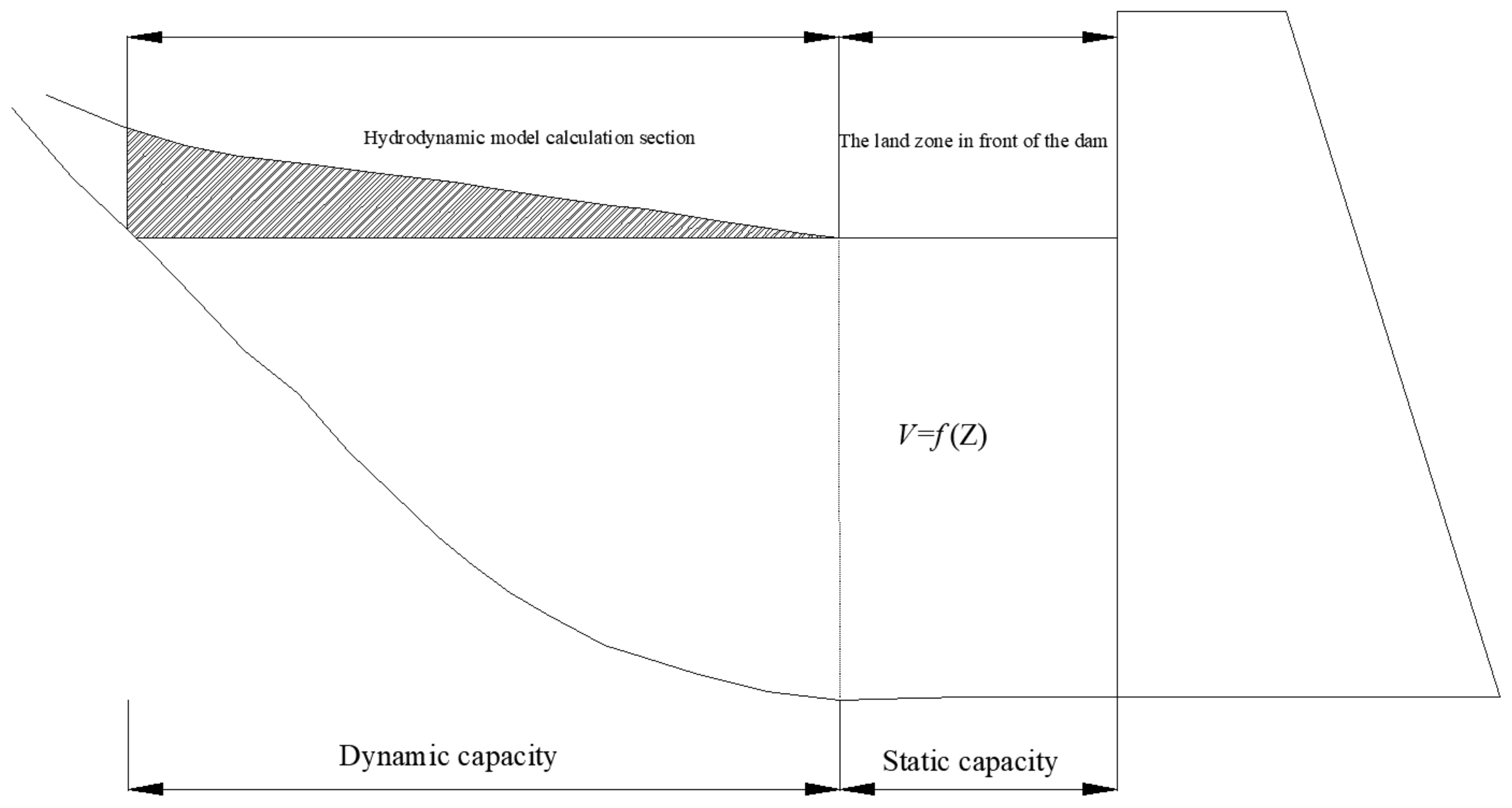
The water surface of river type reservoirs in mountainous areas will form a certain gradient, so the actual water surface is not horizontal, as shown in Figure 2 [30], which leads to the existence of dynamic storage capacity in the reservoir. The water surface in the reservoir area is divided into the land zone in front of dam and a warped section. The accuracy of the calculation results can be guaranteed when using a static storage capacity curve to calculate the storage capacity of the land zone in front of dam section, but the storage capacity will be smaller when calculating the warped section.

The length of the land zone in front of dam is not a constant. There are many factors affect the length of the land zone in front of the dam, such as the water level in front of the dam and inflow discharge.

2.2.2. Combining the Water Balance Calculation and Hydrodynamic Model through the Straight Zone in Front of the Dam

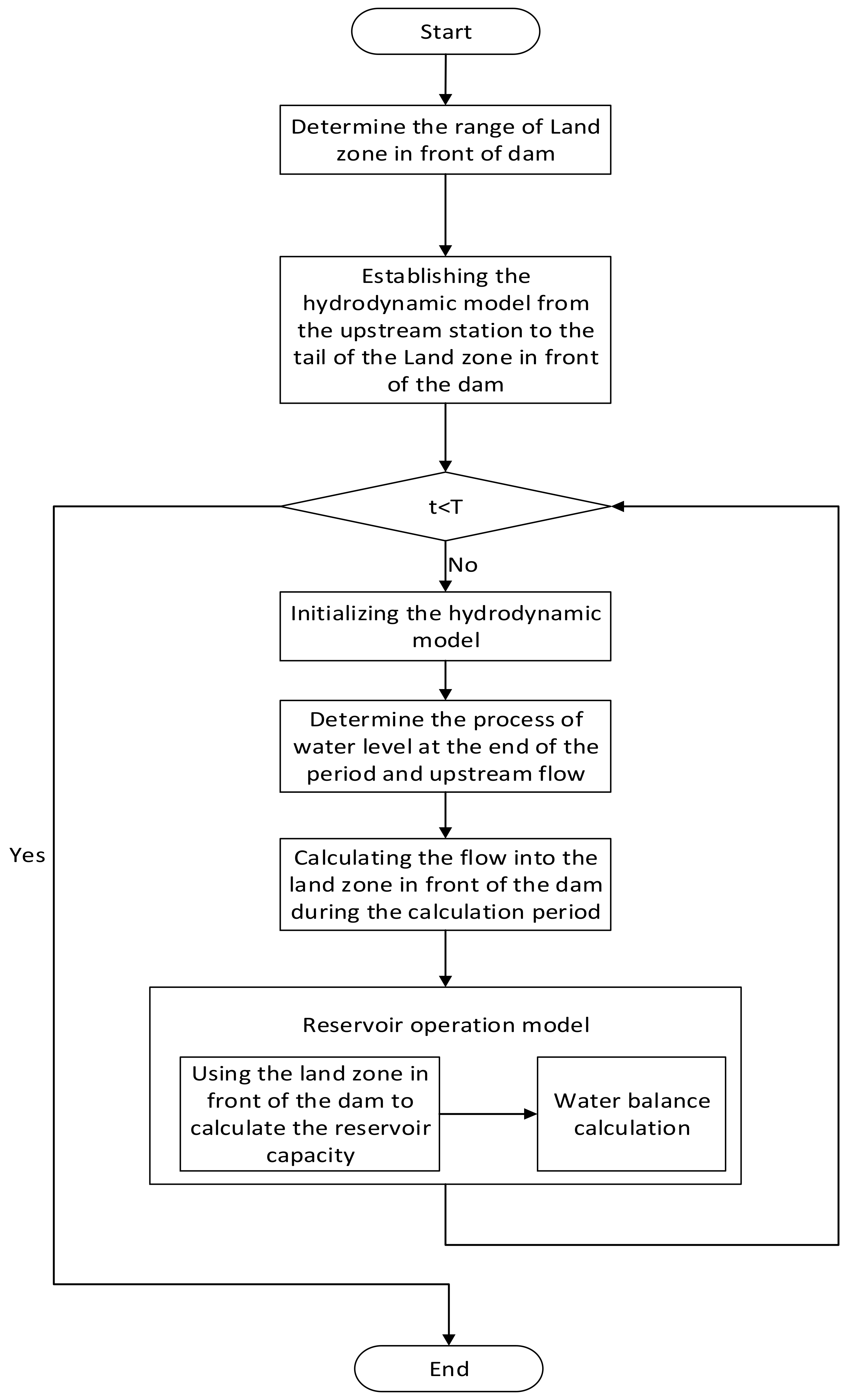
Taking the land zone in front of dam section as the medium, the hydrodynamic model from the upstream prediction station to the end of the land zone in front of the dam is established. The new water balance calculation model proposed in this paper uses the land zone in front of dam to establish a local control body for the water balance calculation. The calculation steps are given below as Figure 3, and all steps are completely automatic:

Step1: determining the range of the land zone in front of the dam by using the hydrological data and the calculation time (T).

Step2: establishing the hydrodynamic model between the upstream hydrological station and the end of the straight zone in front of dam using the measured domain data to establish the hydrodynamic model.

Step3: using the new model to deal with the water balance calculation.

3. Study Area and Data

3.1. Study Area

The Three Gorges Reservoir area, which is located downstream of the Jinsha River was selected as the study area, stretching from Zhutuo to the Three Gorges Dam. The length of the study area is about 760 km. The width of the Jinsha River is between 700 and 1700 m. The Three Gorges Reservoir area is located at the alternation of the second and third levels of topography in China. The geographical conditions are very complex in the Three Gorges Reservoir area, which is surrounded by the Qiling and Daba Mountains in the north and Wu Mountain in the south, and the area comprises 74% mountains, 21.7% hills and 4.3% plains [31]. It is a typical river-type reservoir, and therefore, the Three Gorges Reservoir has great dynamic capacity. The Three Gorges Reservoir area begins at the hydrological station in Zhutuo, as Figure 4 shows, and along the river, there are many hydrological stations, including Cuntan, Qingxichang, Wanxian and Fenghuangshan. The Fenghuangshan hydrological station is close to the dam, so we can use the data from this station on behalf of the water level in front of the dam. There are many small rivers in the reservoir area, such as Quxi River and Modao River, among others. The reservoir area has a subtropical monsoon climate, and the large amount of precipitation in the flood season will lead to interval runoff that cannot be ignored for the whole interval. Relevant studies show that the average contribution of interval inflow to the flood peak in the reservoir area is 20%, and the maximum is close to 50% [32]. The total storage capacity of the Three Gorges Reservoir is 39.3 billion m³, and the flood control storage capacity is 22.15 billion m³. The Three Gorges hydropower station is the largest hydropower station in the world, with a total installed capacity of 22.5 million kW that is produced by thirty-two 700,000 kW generating units and two 50,000 kW auxiliary power units. The normal water level of the Three Gorges Reservoir is 175 m, and the flood limited water level is 145 m.

3.2. Data

To compare the Muskingum method and hydrodynamic model, we used the measured hydrological data from 2005. This is because construction of the Three Gorges Dam was finished in 2006. After the dam was finished, the hydrological station in front of the dam could not measure flow in the river. Similarly, the year the dam was nearly finished also had an impact on the river. Thus, we can use the data from 2005 to compare the differences between the two methods.

To validate the new water balance model proposed in this paper, we used data from 2016 to calibrate the parameters and data from 2017 to test the accuracy of the model parameters. The data used in this article are measured hydrological data that have been reviewed for reliability, consistency and representativeness prior to use. To verify the accuracy of the model with actual operation data, the hourly scale data from 5 July 2019 to 10 July 2019 were combined with the straight section in front of the dam to verify the accuracy of the regulation and storage model.

4. Case Study

4.1. The Comparison between the Hydrodynamic Model and the Muskingum Method

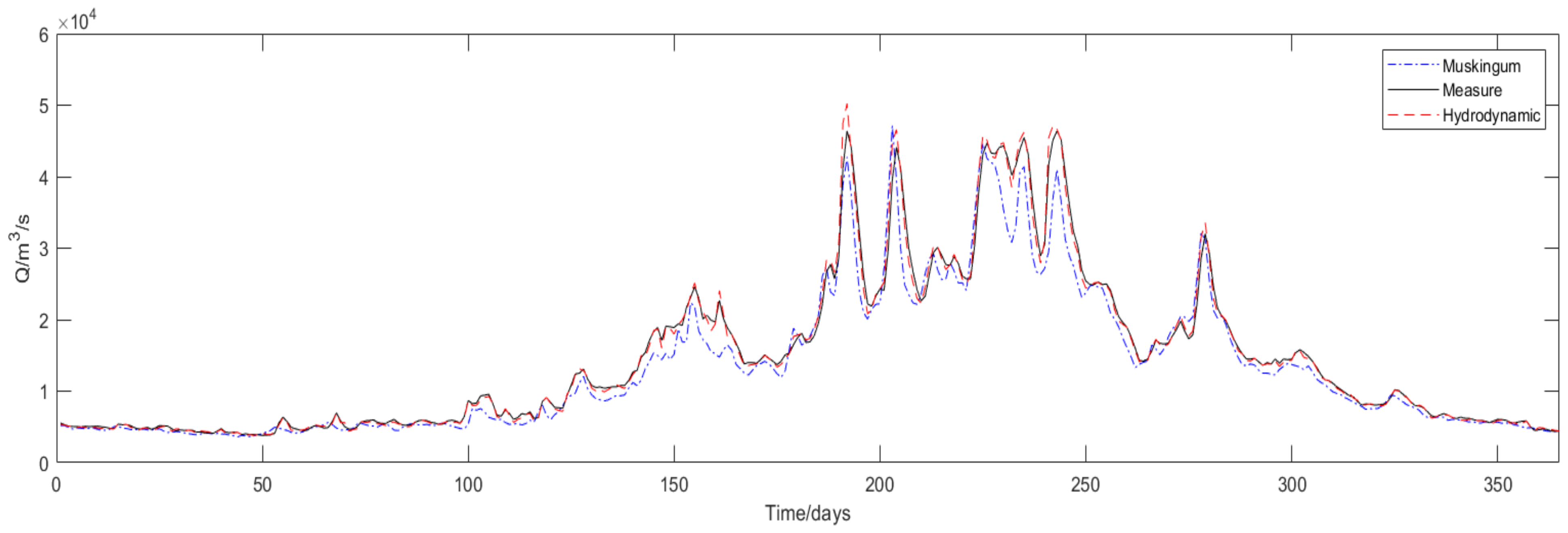
This paper uses Miaohe hydrology station, which is in front of the dam, to compare the two methods. As we can see from Figure 5, there is a large error between the Muskingum method and the measured values. It can be seen from the figure that in the case of multi-peak floods, the Muskingum method and hydrodynamic method are close to the measured values for the first peak, but the flow values from the Muskingum method decreased significantly later. This is because the Muskingum method is a free flow hypothesis, but after the dam was completed, the free flow hypothesis was no longer valid due to the jacking effect of the dam. The average relative error for the Muskingum method was 10.24%, however the average relative error for the hydrodynamic model was 2.79%. During flood season, the average relative error for the Muskingum method was 12.96% compared to 3.57% for the hydrodynamic model. The dam was not completed in 2005, but the Muskingum method still had a larger error than the hydrodynamic method. After the completion of the dam, jacking of the downstream water level was more obvious, so the Muskingum method will no longer be applicable.

4.2. Validation of the Improved Water Balance Calculation Model

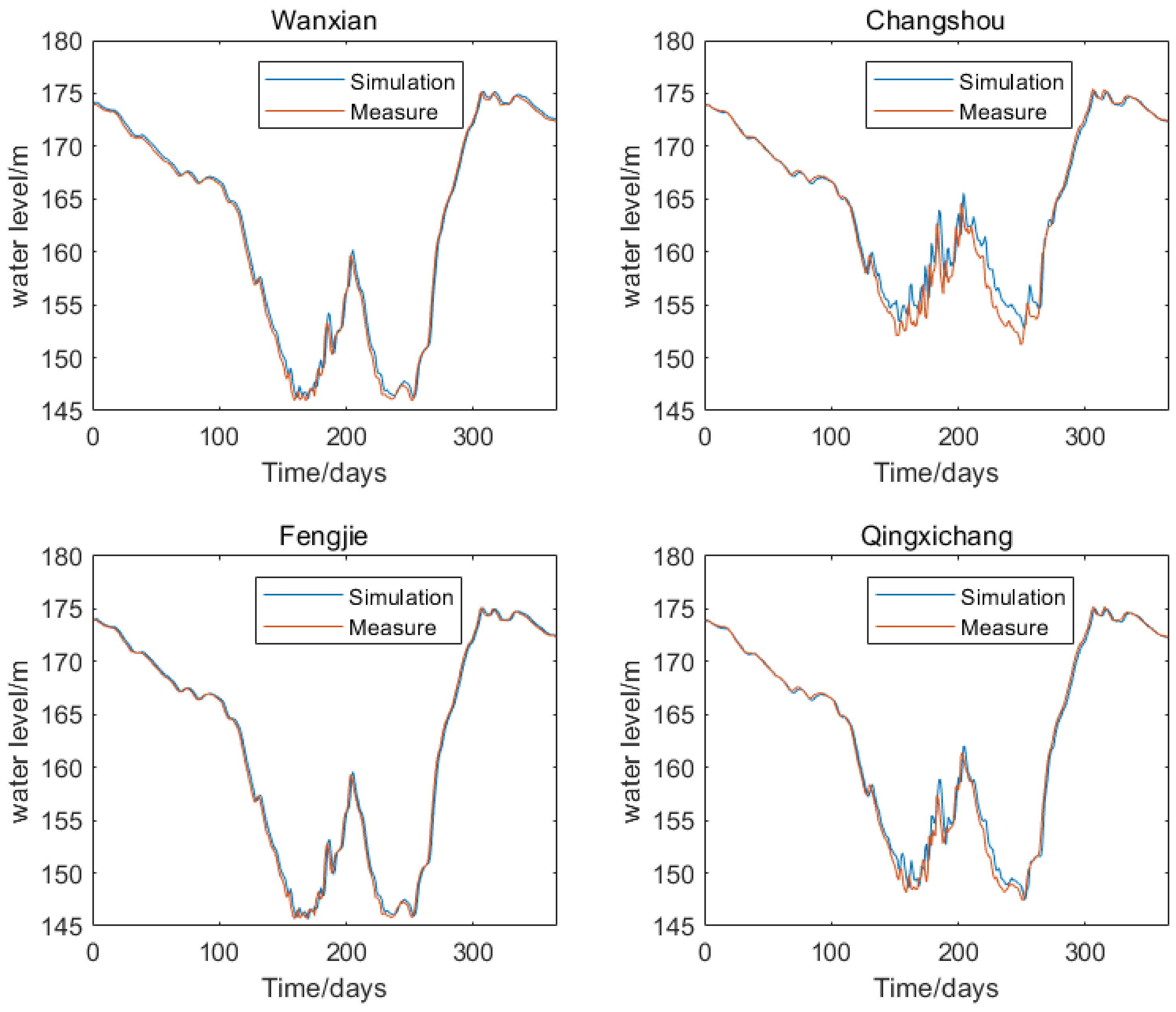
After the completion of the dam, the parameters of the hydrodynamic model needed to be calibrated again. The data from 2016 was chosen for calibration and 2017 data was selected to verify the parameter results. The calibration results are shown in Figure 6.

As can be seen in Figure 6, the closer the hydrological station is to the Three Gorges Dam, the more accurate the simulation results. It can be seen from

Table 1. Statistical comparison results for simulated and measured data at different hydrological sites.

Station Name	Wanxian	Changshou	Fengjie	Qingxichang
Maximum relative error	1.49%	3.54%	1.73%	2.41%
Minimum relative error	0.00%	0.00%	0.00%	0.00%
RMSE	0.32%	0.50%	0.29%	0.36%
Mean value of error	0.22	0.45	0.089	0.17
Variance of error with measured value	0.63	1.87	0.63	0.85

that the relative error for Changshou hydrological station is the largest, reaching 0.5%. It can be seen in Figure 4 that Changshou hydrological station is located at the tail of the Three Gorges Reservoir area. Changshou hydrological station is affected by the dynamic capacity during the flood season, and its water level fluctuates greatly. It can be seen in Figure 6 that the error is more obvious during the flood season, whereas the simulated and measured values are in good agreement during the non-flood season. This is because the manning coefficient differs with the different water levels at Changshou hydrological station, which affects the simulation results. It can be seen from Table 1 that the minimum relative error for the four stations is 0. This is because the Three Gorges Reservoir continues to operate at a water level of 175 m during the dry season and the flow velocity in the entire reservoir area is slow, so the relative error is very small. The calibration results for the Manning coefficient are shown in

Table 2. The Manning coefficient of the river.

Section	Manning Coefficient
Zhutuo, Beibei~Cuntan	0.030~0.038
Cuntan~Changshou	0.038~0.044
Changshou, Wulong~Qingxichang	0.042~0.046
Qingxichang~Zhongxian	0.035~0.038
Zhongxian~Wanxian	0.030~0.038
Wanxian~Fengjie	0.038~0.065
Fengjie~The Three Gorges	0.067~0.078

.

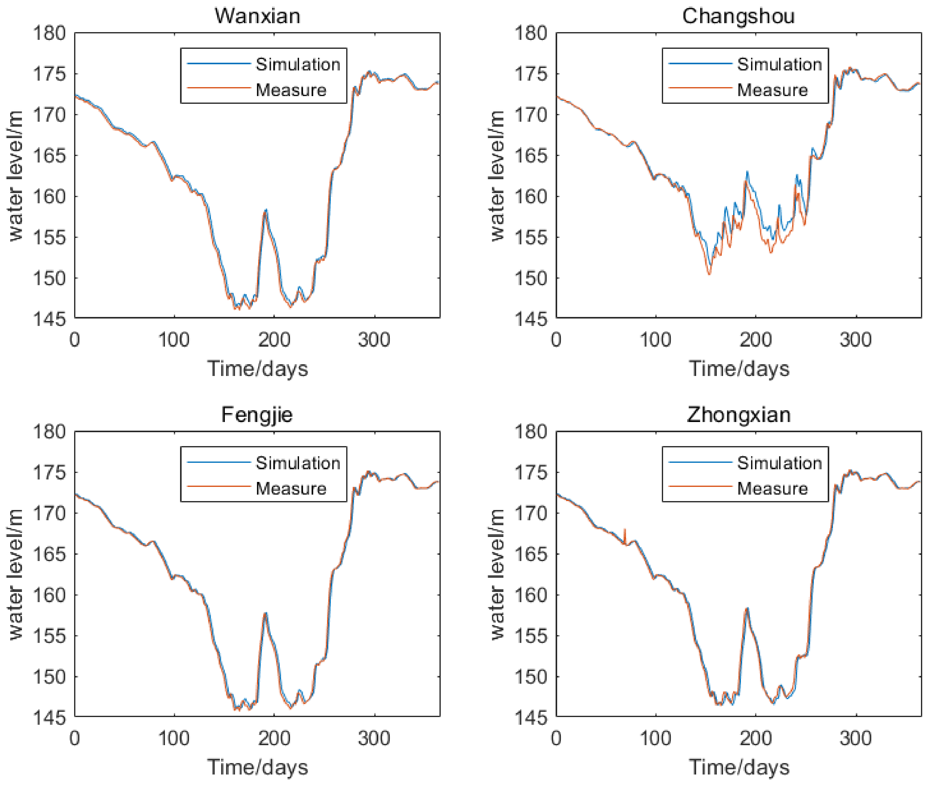
After completing parameter calibration for the hydrodynamic model, the data in 2017 was used to verify the accuracy of the model parameter calibration, and the results are shown in Figure 7.

It can be seen from Figure 7 and

Table 3. Comparison of simulation and measured results for different hydrological stations during the validation period.

Station Name	Wanxian	Changshou	Fengjie	Zhongxian
Maximum relative error	1.80%	2.59%	1.96%	2.04%
Minimum relative error	0.00%	0.00%	0.00%	0.00%
RMSE	0.30%	0.44%	0.26%	0.26%
Mean value of error	0.21	0.39	0.08	−0.01
Variance of error with measured value	0.62	1.04	0.65	0.65

that when considering interval inflow, the measured water level is consistent with the simulated water level, the average relative error at Changshou is only 0.44%, and the relative error for the whole reservoir area is less than 2%. As mentioned previously, Changshou station is located close to the tail of the reservoir. During the flood season, operation of the Three Gorges Reservoir is at the flood limit water level and upstream inflow is large, resulting in obvious dynamic storage capacity in the reservoir. The closer the dynamic storage capacity is to the tail of the reservoir, the greater its impact on reservoir operation activities, so the change is more intense. It can be seen from the figure that considering the interval inflow, the change in water level at Changshou station can be simulated more accurately, indicating that parameter calibration of the hydrodynamic model is more accurate.

4.3. The Model Establishment of Land Zone in Front of the Dam

After parameter calibration, we established a hydrodynamic model between the upstream hydrological station and the end of the land zone in front of the dam. First, we needed to determine where the land zone ended in front of the dam, so we revisited the work of Lu [24].

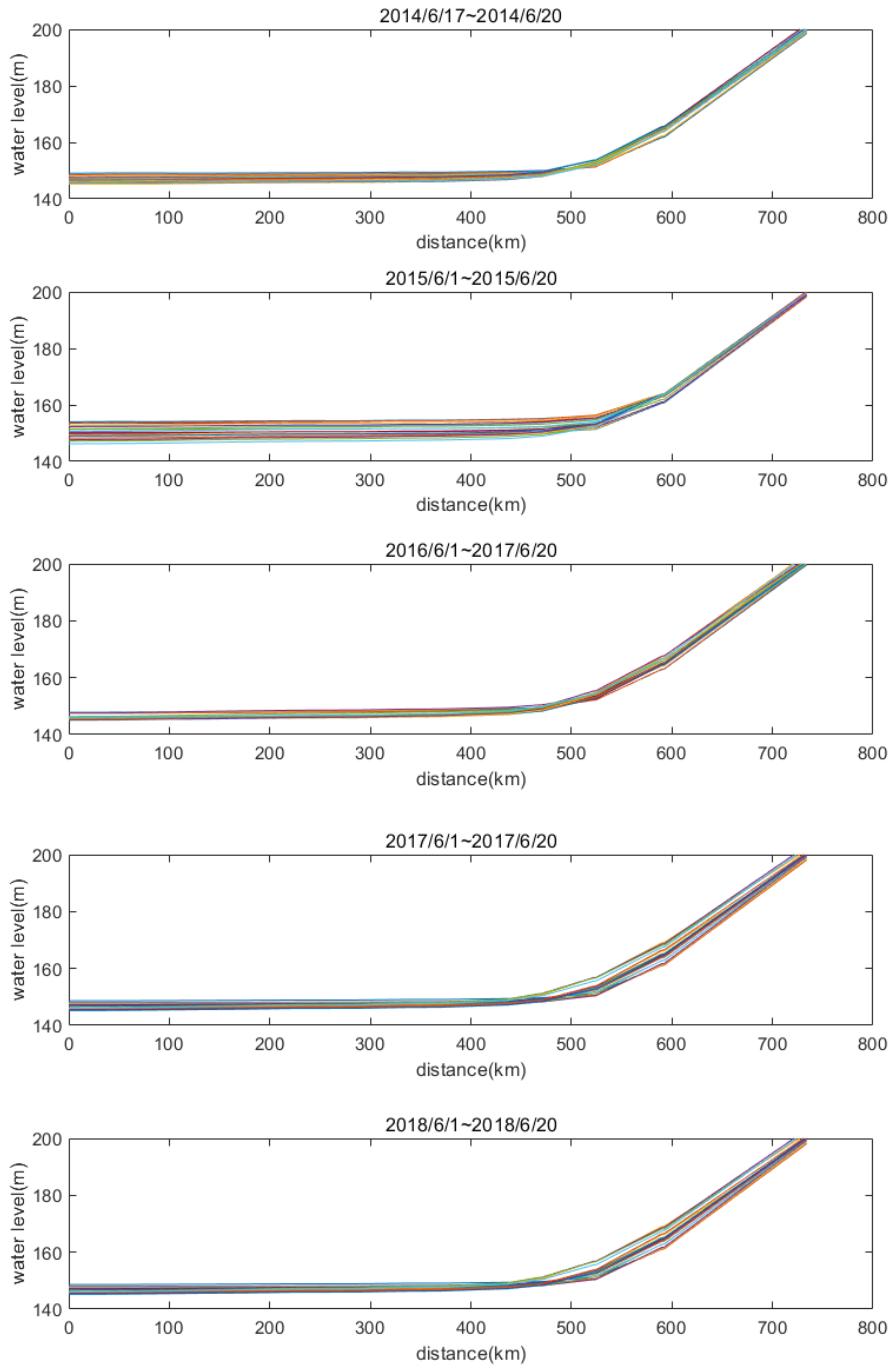
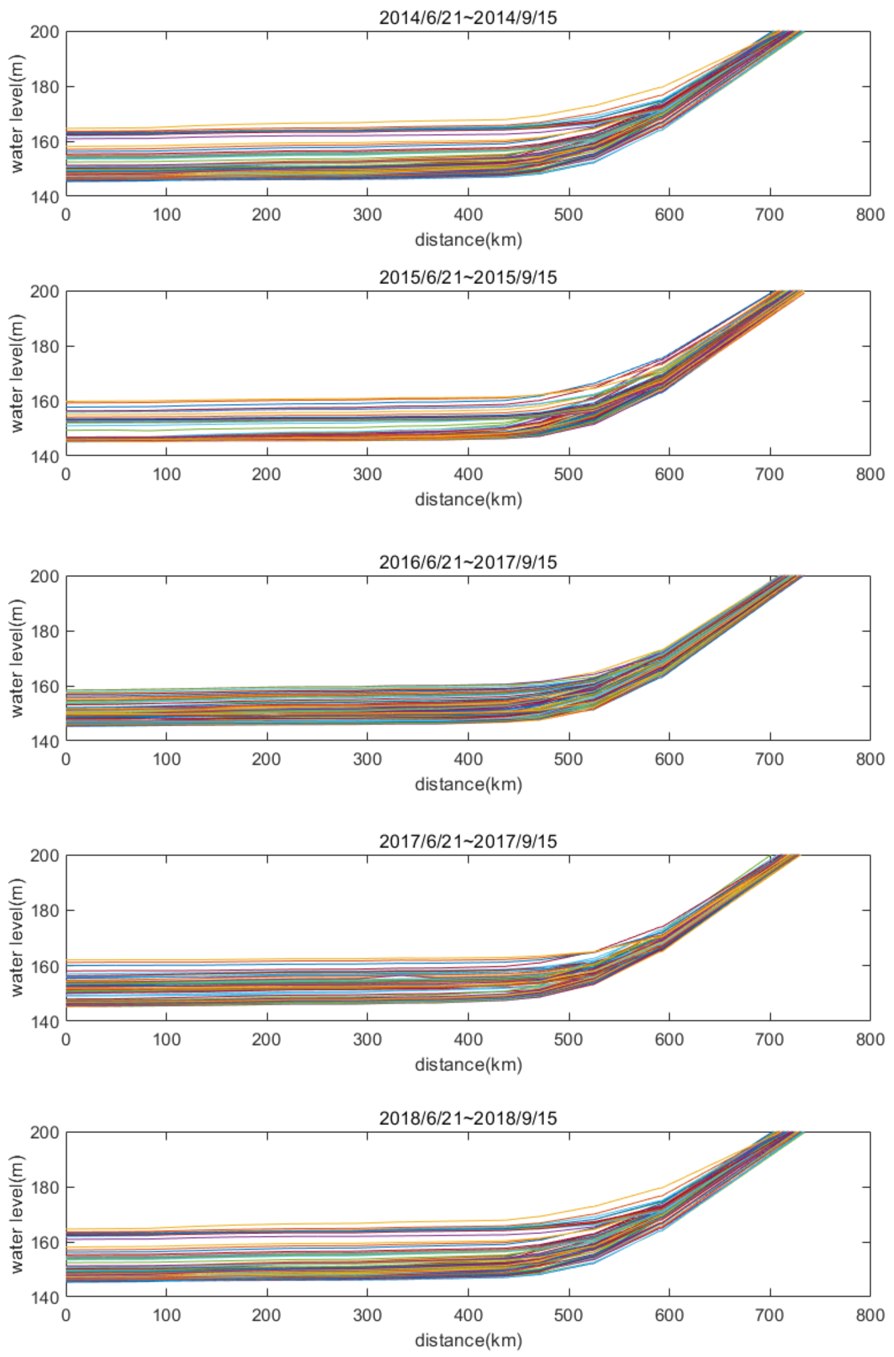
Using measured data from 2014 to 2018, changes in the water surface profile for the Three Gorges Reservoir during the flood season are shown in Figure 8 and Figure 9.

The Three Gorges Reservoir has a huge storage capacity. For every 1 cm change in water level, the water volume in the reservoir can change by millions of cubic meters. From Figure 8 we can see that when the variation range for the water level exceeds 1 cm, the straight section in front of the dam is at its shortest between Wushan and Fengjie hydrological stations and can reach the confluence of Wujiang River at its longest.

The water surface profile during the main flood season is shown in Figure 9. When 1 cm is taken as the judgment standard, the straight section in front of the dam is at its shortest between Badong and Zigui hydrological stations, and at its longest near Qingxichang hydrological station.

We can conclude that the water surface line between the Three Gorges Dam and Badong hydrological station is absolutely horizontal. Thus, for the calculation of water balance, the land zone in front of the dam is taken between the Three Gorges Dam and Badong hydrological station.

Based on the above rules, during short-term fine operation of the reservoir, it is necessary to formulate the daily reservoir operation plan on an hourly scale. The change law for the land zone in front of the dam shows that as the distance from the dam site increases, the changes become more intense. Therefore, an absolute straight section was selected to be combined with the hydrodynamic model. Badong hydrological station is within the confines of the absolute straight level; thus, we decided to use the section between the Three Gorges Dam and Badong hydrological station as the land zone in front of the dam.

Based on the land zone in front of the dam, a hydrodynamic model was established for the region between Zhutuo hydrological station and Badong hydrological station. Using the new water balance model to deal with flood routing through the reservoir, the results were compared with the traditional model.

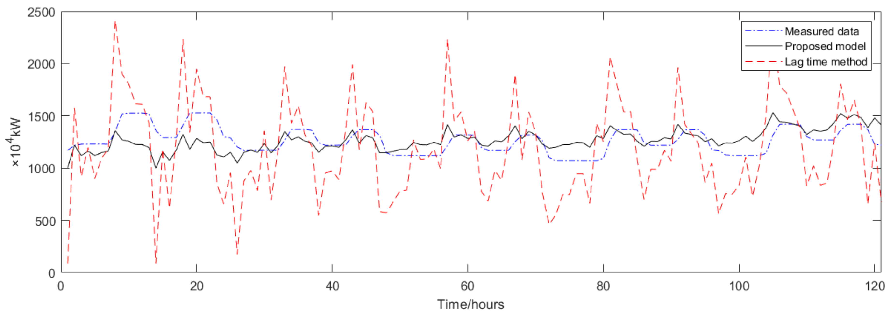
It can be seen from Figure 10 and Figure 11 that after adopting the new water balance calculation model proposed in this paper, the output process of the inversion is relatively consistent with the measured output, but the error for the lag time method is large. It can be seen from

Table 4. Comparison of output inversion error between the time lag method and the new method proposed in this paper.

Indicator	Lag Time Method	Proposed Model
RMSE	25.90%	8.50%

that the average relative error for the lag method is 25.9%, but the average relative error of the new water balance model is only 8.5%.

The reason that the lag time method has a larger error than the new model is that the inflow of the reservoir cannot be calculated accurately, and the flatness of water flow and interval inflow are not considered. Moreover, the control body established by the time lag method cannot accurately calculate the water volume of the reservoir, which has the problem of water imbalance. The new method proposed in this paper combines a hydrodynamic model with the interval inflow, fully considering displacement and flatness in the process of water flow transmission, and the straight section in front of the dam can be used to accurately calculate the reservoir capacity, so the final result is more accurate.

The Three Gorges Dam has a large dynamic capacity during the flood season. Due to the influence of the dynamic storage capacity in the reservoir, calculation of the reservoir storage capacity by the time lag method will be prone to error, and there will be large random factors and great fluctuations that will affect short-term operation of the reservoir. When the model proposed in this paper is used to calculate the output, the output trend is close to the measured trend. However, the traditional time lag method is still used to calculate the interval inflow, and there will be a deviation between the output and the measured output due to random factors during short-term operation of the reservoir.

5. Conclusion and Future Work

This paper proposes a new water balance model that combines a hydrodynamic model with the land zone in front of the dam. The innovations of the proposed model are: (a) compared with the Muskingum method, the hydrodynamic model can provide more accurate inflow for the water balance calculation; (b) by using the land zone in front of the dam, the storage capacity of reservoir can be calculated accurately; (c) compared with the lag time method, the results shows that the new water balance calculation model can calculate water balance more accurately. Using hourly scale data from 5 July 2019 to 10 July 2019, the new water balance calculation model was verified. The main conclusions can be summarized as follows:

(1)

The hydrodynamic model was used to accurately calculate the inflow of the reservoir. Compared with the lag time method, it overcomes the disadvantages caused by only considering flow transposition and not considering flow attenuation. At the same time, it overcomes the disadvantage of the Muskingum method, which cannot consider the influence of reservoir jacking. A case study of the Three Gorges Dam showed that the average relative error for the calculation of inflow was only 2.79%, which can provide more accurate inflow data for refinement of the reservoir.

(2)

Focusing on the problem of large errors in the calculation of reservoir storage capacity caused by dynamic capacity in the flood season, this paper introduces the land zone in front of the dam. The tail of the land zone in front of the dam and its upstream are all regarded as the river channel, and only the straight section in front of the dam is regarded as the reservoir so as to realize the accurate calculation of reservoir capacity.

(3)

In this paper, the land zone in front of the dam was coupled with a hydrodynamic model for the first time, and a new water balance calculation model is proposed. By coupling a one-dimensional hydrodynamic model with the reservoir operation model in front of the dam, an output inversion calculation was carried out for the Three Gorges Dam as the research object. The research results show that the accuracy of the proposed method was significantly improved compared with the traditional reservoir operation model, since the RMSE of the new method was only 8.5%.

The model proposed in this paper can be used for the short-term refined operation of reservoirs to provide more accurate values for inflow and storage capacity. In the future, according to the variation law for the land zone in front of the dam, the dynamic land zone in front of the dam will be used to calculate reservoir capacity more accurately.

References

- Labadie, J.W. Optimal operation of multireservoir systems: State-of-the-art review. J. Water Resour. Plan. Manag. 2004, 130, 93–111. [Google Scholar] [CrossRef]
- Ren, K.; Huang, S.; Huang, Q.; Wang, H.; Leng, G.; Wu, Y. Defining the robust operating rule for multi-purpose water reservoirs under deep uncertainties. J. Hydrol. 2019, 578, 124134. [Google Scholar] [CrossRef]
- Feng, Z.K.; Liu, S.; Niu, W.J.; Li, S.S.; Wu, H.J.; Wang, J.Y. Ecological operation of cascade hydropower reservoirs by elite-guide gravitational search algorithm with Lévy flight local search and mutation. J. Hydrol. 2020, 581, 124425. [Google Scholar] [CrossRef]
- Niu, W.J.; Feng, Z.K.; Liu, S.; Chen, Y.B.; Xu, Y.S.; Zhang, J. Multiple hydropower reservoirs operation by hyperbolic grey wolf optimizer based on elitism selection and adaptive mutation. Water Resour. Manag. 2021, 35, 573–591. [Google Scholar] [CrossRef]
- Yu, L.; Li, Y.P.; Huang, G.H. A fuzzy-stochastic simulation-optimization model for planning electric power systems with considering peak-electricity demand: A case study of Qingdao, China. Energy 2016, 98, 190–203. [Google Scholar] [CrossRef]
- Lv, S.; He, W.; Zhang, A.; Li, G.; Luo, B.; Liu, X. Modelling and analysis of a novel compressed air energy storage system for trigeneration based on electrical energy peak load shifting. Energy Convers. Manag. 2017, 135, 394–401. [Google Scholar] [CrossRef]
- Qiu, H.; Zhou, J.; Chen, L.; Zhu, Y. Multiple Strategies Based Salp Swarm Algorithm for Optimal Operation of Multiple Hydropower Reservoirs. Water 2021, 13, 2753. [Google Scholar] [CrossRef]
- Chen, X.; Zhou, J.; Jia, B.; Yang, X.; Zhou, C. Characterizing the hydraulic connection of cascade reservoirs for short-term generation dispatching via Gaussian process regression. IEEE Access 2020, 8, 145489–145502. [Google Scholar] [CrossRef]
- Ji, C.; Li, C.; Wang, B.; Liu, M.; Wang, L. Multi-stage dynamic programming method for short-term cascade reservoirs optimal operation with flow attenuation. Water Resour. Manag. 2017, 31, 4571–4586. [Google Scholar] [CrossRef]
- Zhang, Y.; Liu, Y.; Wu, Y.; Ji, C.; Ma, Q. Short-term optimal operation of cascade reservoirs considering dynamic water flow hysteresis. Water 2019, 11, 2098. [Google Scholar] [CrossRef] [Green Version]
- Kim, J.H.; Geem, Z.W.; Kim, E.S. Parameter estimation of the nonlinear muskingum model using harmony search 1. J. Am. Water Resour. Assoc. 2001, 37, 1131–1138. [Google Scholar] [CrossRef]
- Todini, E. A mass conservative and water storage consistent variable parameter Muskingum-Cunge approach. Hydrol. Earth Syst. Sci. 2007, 11, 1645–1659. [Google Scholar] [CrossRef] [Green Version]
- Huang, Y.; Liang, Z.; Singh, V.P.; Hu, Y.; Li, B.; Wang, J. A coupled dynamic system inversion model for higher accuracy in flood forecasting. Water Resour. Res. 2022, 58, e2021WR030531. [Google Scholar] [CrossRef]
- Hu, D.; Lu, C.; Yao, S.; Yuan, S.; Zhu, Y.; Duan, C.; Liu, Y. A prediction–correction solver for real-time simulation of free-surface flows in river networks. Water 2019, 11, 2525. [Google Scholar] [CrossRef] [Green Version]
- Toro, E.F. Shock-Capturing Methods for Free-Surface Shallow Flows; John Wiley & Sons: New York, NY, USA, 2001. [Google Scholar]
- DHI. A Modelling System for Rivers and Channels, Reference Manual; DHI: Horsholm, Denmark, 2014. [Google Scholar]
- Li, Q.; Liang, Q.; Xia, X. A novel 1D-2D coupled model for hydrodynamic simulation of flows in drainage networks. Adv. Water Resour. 2020, 137, 103519. [Google Scholar] [CrossRef]
- Ying, X.; Wang, S.S. Improved implementation of the HLL approximate Riemann solver for one-dimensional open channel flows. J. Hydraul. Res. 2008, 46, 21–34. [Google Scholar] [CrossRef]
- Casulli, V. Semi-implicit finite difference methods for the two-dimensional shallow water equations. J. Comput. Phys. 1990, 86, 56–74. [Google Scholar] [CrossRef]
- Hu, D.; Yao, S.; Duan, C.; Li, S. Real-time simulation of hydrodynamic and scalar transport in large river-lake systems. J. Hydrol. 2020, 582, 124531. [Google Scholar] [CrossRef]
- Walters, R.A.; Casulli, V. A robust, finite element model for hydrostatic surface water flows. Commun. Numer. Methods Eng. 1998, 14, 931–940. [Google Scholar] [CrossRef]
- Martyushev, D.A. Improving the geological and hydrodynamic model of a carbonate oil object by taking into account the permeability anisotropy parameter. J. Min. Inst. 2020, 243, 313. [Google Scholar] [CrossRef]
- Potashev, K.A.; Akhunov, R.R.; Mazo, A.B. Calculation of the flow rate between wells in the flow model of an oil reservoir using streamlines. Georesursy 2022, 24, 27–35. [Google Scholar] [CrossRef]
- Lu, C.W. Research and Application on Comprehensive Flood Control Dispatching of Reservoir Groups and Flood Detention Areas. Ph.D. Thesis, Huazhong University of Science and Technology, Wuhan, China, 2019. [Google Scholar]
- Yermekov, R.I.; Merkulov, V.P.; Chernova, O.S.; Korovin, M.O. Features of permeability anisotropy accounting in the hydrodynamic model. J. Min. Inst. 2020, 243, 299. [Google Scholar] [CrossRef]
- Martyushev, D.A. Rock stress state influence on permeability of carbonate reservoirs. Bull. Tomsk Polytech. Univ. Geo Assets Eng. 2020, 331, 24–33. [Google Scholar] [CrossRef]
- Robert, A. A stable numerical integration scheme for the primitive meteorological equations. Atmos. Ocean 1981, 19, 35–46. [Google Scholar] [CrossRef] [Green Version]
- Robert, A. A semi-Lagrangian and semi-implicit numerical integration scheme for the primitive meteorological equations. J. Meteorol. Soc. Jpn. Ser. II 1982, 60, 319–325. [Google Scholar] [CrossRef] [Green Version]
- Ren-Jun, Z. The Xinanjiang model applied in China. J. Hydrol. 1992, 135, 371–381. [Google Scholar] [CrossRef]
- Zhang, S.; Jing, Z.; Yi, Y.; Wu, Y.; Zhao, Y. The dynamic capacity calculation method and the flood control ability of the Three Gorges Reservoir. J. Hydrol. 2017, 555, 361–370. [Google Scholar] [CrossRef]
- Yan, Q.; Jing, Z.; Xia, Z.; Zhang, S. Flood Control Capacity of the Three Gorges Project for Different Frequency Floods. Environ. Eng. Sci. 2021, 38, 1195–1205. [Google Scholar] [CrossRef]
- Song, Z.; Liang, S.; Feng, L.; He, T.; Song, X.P.; Zhang, L. Temperature changes in three gorges reservoir area and linkage with three gorges project. J. Geophys. Res. Atmos. 2017, 122, 4866–4879. [Google Scholar] [CrossRef]
Figure 1.
The control volume and grid used in the hydrodynamic model.
Figure 2.
Schematic diagram of the straight section in front of a dam.
Figure 3.
The calculation steps for the new water balance model.
Figure 4.
Schematic diagram of the study area.
Figure 5.
Comparison of the results from the Muskingum method and the hydrodynamic model with measured data from 2005.
Figure 6.
Comparison of the results from the simulation with measured data from 2016.
Figure 7.
Comparison of the simulation and measured results during the verification period for each hydrological station.
Figure 8.
Water surface line during the early flood season from 2014 to 2018.
Figure 9.
Water surface line during the main flood season from 2014 to 2018.
Figure 10.
Comparison of the results from the traditional method with the proposed model.
Figure 11.
Comparison of the results from the proposed method with the measured data.