Temperature Modeling, a Key to Assessing Impact on Rivers Due to Urbanization and Climate Change

Abstract

With widespread ongoing urbanization and as climate change continues, the importance of protecting the water quality of streams and lakes is intensifying. However, while many water quality constituents in lakes and rivers are of overall interest, water temperature is a ‘key’ variable as temperature influences mixing within a waterbody, influences the acceptability of the habitat for flora and fauna, and serves as a guide to the general health of a stream. To enable the assessment, a physics-based, deterministic hydraulic and heat-balance modeling procedure using the combination of MIKE SHE, MIKE HYDRO and ECO Lab is described to assess heat transfer magnitudes in portions of the Credit River, Ontario. Changes in instream temperature regimes are examined, including both frequency and spatial extent, providing insights into the impacts of urbanization in terms of seasonal temperature shifts arising from land use changes. For flow and temperature regimes, Nash–Sutcliffe model efficiency coefficient (NSE) values of 0.49 and 0.955 were achieved, respectively, for current threshold conditions. Durations of temperature increases from threshold levels indicate that land use changes from current agriculture conditions to urbanization may change stream water temperatures for 9% of the time by 1 °C, and 2% of the time by 2 °C for distances of 1000 m downstream, because of land use change from agriculture to low-density urbanization, and for 20% of the time by 1 °C, and 4% of the time by 2 °C at distances of 1000 m downstream with land use change to high-density urbanization. With climate change RCP 4.5 Scenario in 2050 (Base, for a Wet Year—2017), the continuous amount of time the stream water temperature remains at elevated temperatures of more than 3 °C (from 5000 m to 25,607 m from the most upstream point of Fletchers Creek) for a distance of 20,000 m is more than 13 h. These elevations in temperature may have serious implications for flora and fauna in the creek, particularly impacting the cold-water and mixed-water fish species.

1. Introduction

With widespread and extensive urbanization, and as climate change continues, the challenges will increase to protect the water quality of ambient lakes and rivers. A fundamental part of the challenges involves ensuring there is sufficient accuracy implicit in assessing the impacts of urbanization and climate change, meaning there is need for a mathematical model able to assess the degree of change, and the potential merits of various protective actions. However, to ensure that such needs are correctly responded to, there is a key need to ensure the capability of a model is sufficiently robust to accurately assess the impacts.

While many water quality constituents in lakes and rivers are of overall interest, water temperature is a ‘key’ variable as temperature influences mixing within a waterbody, influences the acceptability of the habitat for flora and fauna, and serves as a guide to the general health of a stream. Furthermore, given that climate change is ongoing and land use changes continue, temperature is widely considered as a ‘master’ water quality variable due to its influence on a host of physical, chemical, and biological processes [1].

There are preferred temperature ranges for aquatic species such as fish, insects, zooplankton, phytoplankton, and more. Hence, when river flows are low, the assimilative heat capacity of rivers is reduced and less energy is required to warm the water, which in turn influences kinetic reactions. As a result, for streams with low flows due to their having less thermal mass, stream temperatures may react to atmospheric conditions more rapidly than streams with high flows [2]. Furthermore, as Fabris et al. [3] indicated, increasing water temperatures in many areas are in response to climate change with recent studies showing trends in local air temperature that are consistent with the temperature of rivers.

Given the array of important dimensions referred to above, the ability to characterize water temperatures in a river is a critical water parameter for aquatic systems. Hence, the ability to characterize the extent to which urbanization, water depth and climate change may elevate river temperatures, indicating there are many dimensions which are important. These include when precipitation strikes impervious surfaces exposed to sunlight; this may induce short-circuiting in ponds/lakes/rivers (e.g., [4,5,6,7]). As another example, many species are intolerant of thermal stress meaning that river temperature increases associated with climate change are especially important in high-latitude and high-altitude areas where freshwater ecosystems have adapted to lower temperatures.

Widespread interest exists to explore the capabilities to model temperatures arising from such features as climate change and urbanization (e.g., [8,9,10,11,12]). However, practitioners and regulators are challenged when translating the complex technologic and conceptual advances in river temperature research, into improvements in management practices. These circumstances are expected to be exacerbated by further increases in water abstractions and the impacts arising from urbanization. Water-temperature-modeling research has experienced important advances, from developing new monitoring and modelling tools, to better understanding the mechanisms of temperature feedback with biogeochemical and ecological processes. Deas et al. [13], Cassie [14] and Dugdale et al. [15] reviewed various process-based and linear and logistic regression and stochastic models. While several process-based stream temperature models are available, they are not physics-based models. As well, there are also now many machine-learning models becoming available (e.g., [16,17,18]), but these model types for stream temperature modeling have significant limitations due to the availability of data.

Due to the limitations expressed above, this paper describes use of deterministic (also known as process-based, physics-based and mechanistic) models. An evaluation of quantitative (physics-based) models, namely MIKE SHE, MIKE HYDRO and ECO Lab with all three being parts of the MIKE modeling system, each with individual aspects allowing assessment of change in land use and climate change. MIKE SHE is a physics-based deterministic model and able to dynamically integrate with a river model, MIKE HYDRO. In turn, MIKE HYDRO is a user-customizable water quality model, and ECO Lab enables simulation of temperature regimes in sub-catchments [19,20]. In this research, the utility of the MIKE modeling system was evaluated by application to a portion of the Credit River in Ontario, Canada. Using MIKE SHE as a watershed model to characterize the overland water movement, the unsaturated zone and the saturated zone enable characterization of water quantities, to provide lateral inflows from overland, saturated zone, and saturated zone drain contributions as input to MIKE HYDRO model. Next, MIKE HYDRO, a hydrodynamic model which uses an implicit, finite difference scheme to characterize unsteady flows in rivers, is coupled with MIKE SHE and linked with ECO Lab (the heat balance) model component, to simulate stream water temperature [21].

In this research, two land use change scenarios are evaluated: Scenario-1 by replacing the current agriculture and barren land use area to low-density urban land use change (henceforth called Scenario-1) and by replacing the current agriculture and barren land use area with high-density urban land use change (henceforth called Scenario-2), the changes in stream water temperature were used to characterize over distances along the stream to assess the impact of land use change, and (3) the impacts of climate change. MIKE-SHE relies upon mathematical representations of the underlying physics of heat exchange between the river and the surrounding environment and heat exchanges occurring within a waterbody [15,22]. These model types are more appropriate for assessing alternative impact scenarios from anthropogenic effects (e.g., impact of reservoirs, thermal discharges and assessing the impact of deforestation). They allow the estimation of water temperature at various scales, from focal points such as gauging stations to multiple locations throughout a watershed [14]. As a result, process-based models require significant observed data (e.g., catchment characteristics and geometry, and comprehensive meteorological data and hydraulic properties), making them relatively complex, plus their effective use is further limited due to scarcity of data which represents a common, major concern.

MIKE SHE links hydrology and hydrodynamics components (e.g., snowmelt, interception, overland flow, infiltration into soils, evapotranspiration from vegetation and subsurface flow) to characterize water quality impacts [23]. Coupling to MIKE HYDRO, the one-dimensional surface water model provides simulation of the fully dynamic channel flows and control structures [24,25] along with the user-customizable water quality model, ECO Lab. As a result, MIKE SHE can express the spatial heterogeneity of nature, while integrating surface–subsurface hydrologic processes on a physical basis. Examples of usage include [26] who reported that MIKE SHE has been utilized for international river basins (e.g., [24,27,28]), on catchments with areas of hundreds to thousands of km² [29,30,31,32], and small (<50 km²) catchments and individual wetlands [24,33,34,35,36].

2. Modelling Approach and Case Study Description

2.1. Temperature Regime Change in Fletchers Creek with Land Use Changes—A Case Study

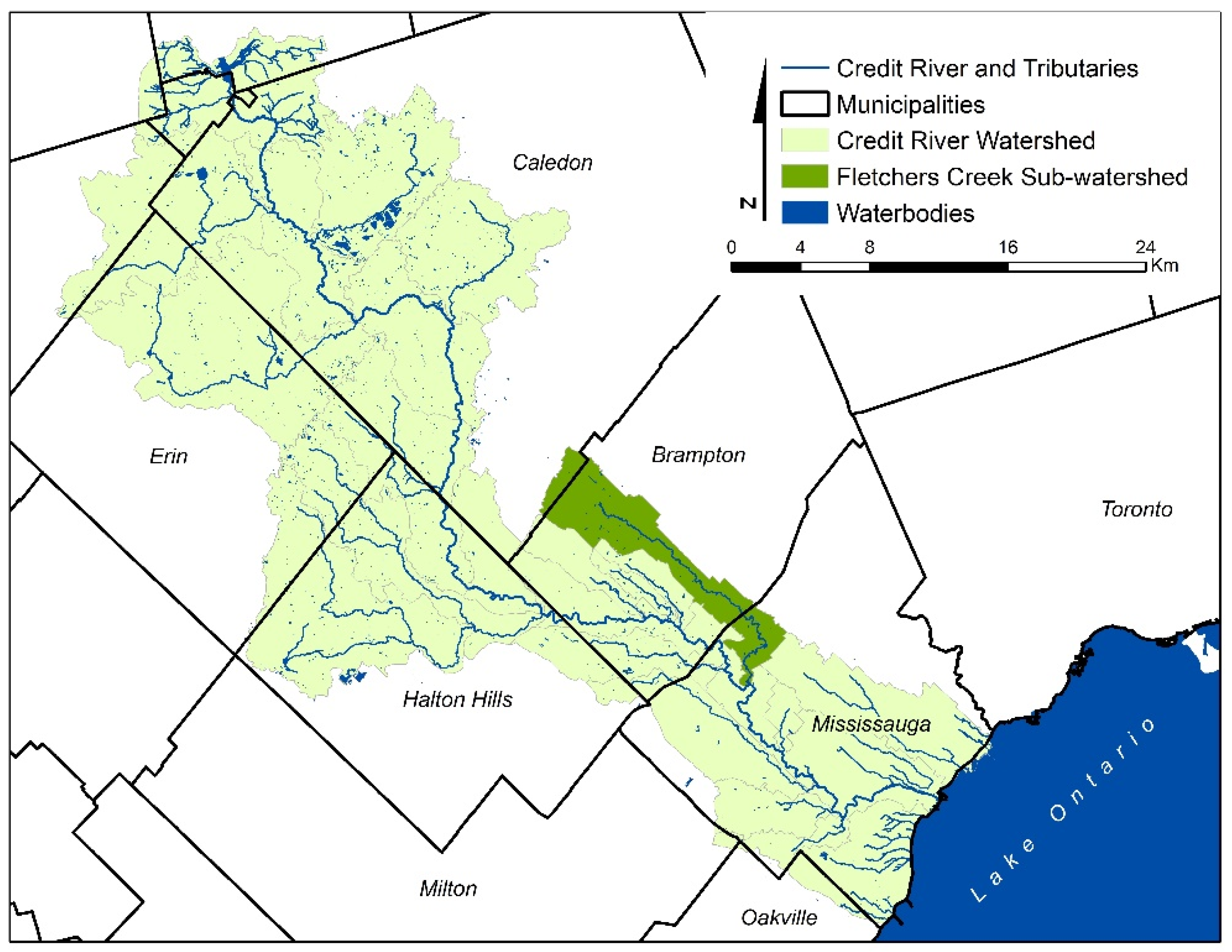
To assess changes in stream temperatures in receiving waterbodies to changes in adjacent land use (e.g., transformation from rural to urban), an application to Fletchers Creek, a watershed of the Credit River as shown in Figure 1, is described. Fletchers Creek watershed lies inside the lower third of the Credit River watershed, draining an area of ~45 km², 18 km in length. Currently, this area is predominantly agricultural, but planning is underway to urbanize significant additional portions of adjacent lands. Currently, this area has a diverse land use including some existing urban area, lands undergoing construction, and some agricultural areas.

Climate characterization includes air temperature, precipitation, evapotranspiration, humidity, wind speed, and degree-day coefficient. The climate of Fletchers Creek is characterized by mild winters and hot summers, with each of the four seasons having different precipitation patterns. The mean annual precipitation is 793 mm based on 30 years of climate data [37]. The driest months of the year are usually January through to March (42.6 to 57.1 mm/month), and the wettest months are typically May through September (72.5 to 79.6 mm/month). Based on a 30-year record, precipitation occurs, on average, 146 days of the year, and ~11 to 13 days per month. High runoff conditions may occur during the months of November, December, February, and March when the ground is saturated and/or frozen and when precipitation is characterized more as rainfall [37].

The observed precipitation and evapotranspiration data of Fletchers Creek sub-watershed from years 2008 to 2018 are shown in Table S1 in Supplementary. The annual precipitation ranged from 609 mm to 1026 mm and the annual evapotranspiration ranged from 599 mm to 770 mm.

The distribution of various types of soil is presented in Table S2. The soils of Fletchers Creek watershed are primarily clay loam and clay. The current land uses of Fletchers Creek are shown in

Table 1. Land Use Characteristics in Fletchers Creek Sub-watershed.

Code	Sub 05 Land Use	Area [ha]	Area %
2	Agriculture	506	10.6
3	Aquatic	40	0.84
4	Barren	227	4.73
5	Grass/Forb	388	8.1
6	Manicured	368	7.68
7	Paved	218	4.55
8	Shrub	40	0.84
9	Treed—Coniferous	2	0.04
10	Treed—Deciduous	226	4.71
11	Treed—Mixed	4	0.07
12	Urban—High	722	15.1
13	Urban—Low	21	0.43
14	Urban—Medium	2030	42.4
	Total:	4793	100

.

2.2. Model Set-Up for Coupled MIKE SHE/MIKE HYDRO/ECO Lab

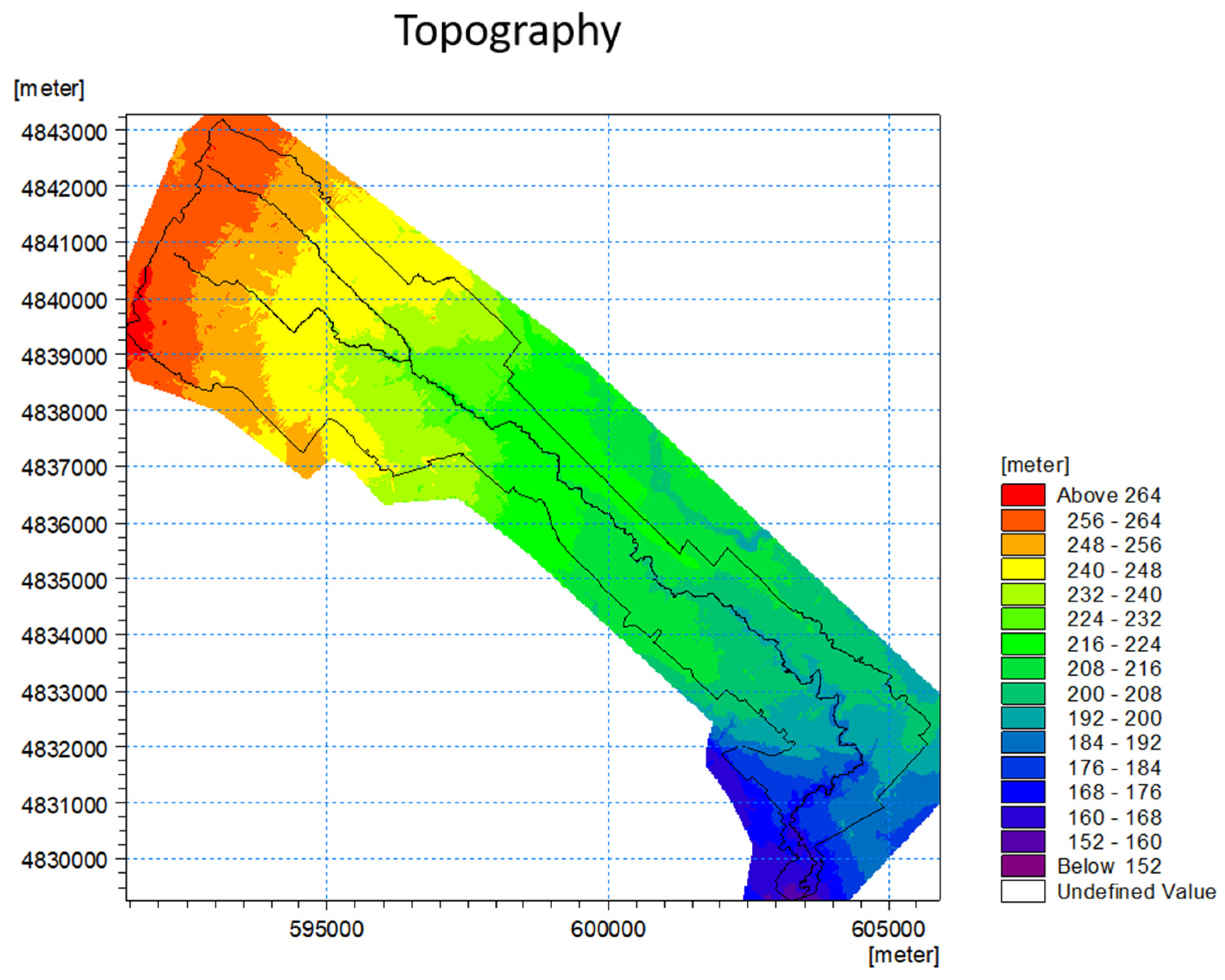
The study area and model domain were defined using a polygon shapefile with a model cell size of 50 m by 50 m. The surface elevation was defined by a Digital Elevation Model (DEM) with resolution of 1 m from CVC Lidar “bare earth” DEM owned by Airborne Imaging. The topography of Fletchers Creek and the hydrologic network are shown in Figure 2.

Using the entire Digital Elevation Model (DEM), grids and interpretation of various land uses, soil, overland, unsaturated zone, river network and saturated zone properties were determined using MIKE SHE. The river network was characterized by a total of 62 cross-sections. Land uses in the model setup were characterized using Leaf Area Index, Root Depth, and Crop Coefficient (Kc).

2.3. ECO Lab Model

The ECO Lab (for heat balance) model [38] was modified in this research by adding a volume coefficient to the water quality module in MIKE HYDRO. For the complete simulation to run, two MIKE HYDRO models were used, one for the hydrodynamics of the water within the stream network and the second for the advection–dispersion within the stream network. The heat balance portion of the simulation was calculated through the advection–dispersion model. The ECO Lab model was used for simulating heat transfer between the water body and atmosphere and income flows from surface and saturated zones. The temperature modeling included the atmospheric heat balance terms and surface water–groundwater heat exchange flux by both conduction and advection. The description is presented in S1 in Supplementary. The ECO Lab model calculates the change in water temperature derived from multiple components. Changes in temperature per time step were calculated as:

$$\frac{\mathrm{dT}}{\mathrm{dt}}=\frac{\mathrm{Qnet}\times \mathrm{SArea}\times 86400}{\mathrm{Cw}\times \mathsf{\rho }\mathrm{w}\times \mathrm{Volume}}$$

(1)

where Qnet is the sum of the incoming and outgoing energy (shortwave, longwave, convective, latent and sources) in J/m² s

SArea is the surface area (m²);

Cw is the specific heat of water (J/kg/C);

ρw is the density of water (kg/m³);

Volume is the volume of water of the calculation point (m³);

T is temperature in °C.

MIKE HYDRO (and ECO Lab) was used to model the heat balance within the stream. Since the heat balance in the stream is dependent on the temperature of lateral sources entering into the river, MIKE SHE was used to characterize the flow quantities of inputs re overland flow, base flow and saturated drain flow along with their respective temperatures. Projections of changes in stream temperature were modeled as heat fluxes from 5 different sources, arising as input to the river):

(1)

Atmospheric heat from sunlight, direct to the river;

(2)

Thermal impacts passed from (i) temperature of overland flow, (ii) stormwater flow from storm sewer systems, (iii) temperature of base flow from all the aquifer layers, and (iv) temperature of drain flow. Since every land use requires different calibrated numbers for detention storage and runoff coefficients, quantities of water in overland flow, base flow and saturated zone drain flow were calculated using the results of simulation model runs of water movement for Scenarios-1 and -2 used in this application.

In this research, overland flow temperatures were characterized by the air temperature (corrected to never go below 4 °C). For the temperature of the base flow and saturated zone drain water, the 25th, 50th or 75th percentile of the observed water temperatures series at monitoring point of 2 line were calibrated as shown in Figure 3 in Fletchers Creek. The ECO Lab model was implemented using a process equation solver ECO Lab Heatbalance M1D_PlaceholderV13.ecolab [39]. A comprehensive description of the Heat Balance model component can be found in [10].

ECO Lab Model Setup

ECO Lab model setup was accomplished by dynamically coupling the ECO Lab with MIKE SHE and MIKE HYDRO. ECO Lab was employed using the seasonality of the air temperature, humidity, wind speed at 10 m (W10), number of sunshine hours (Nsun) and the shortwave solar radiation (SolRad), observed solar radiation as input to the model.

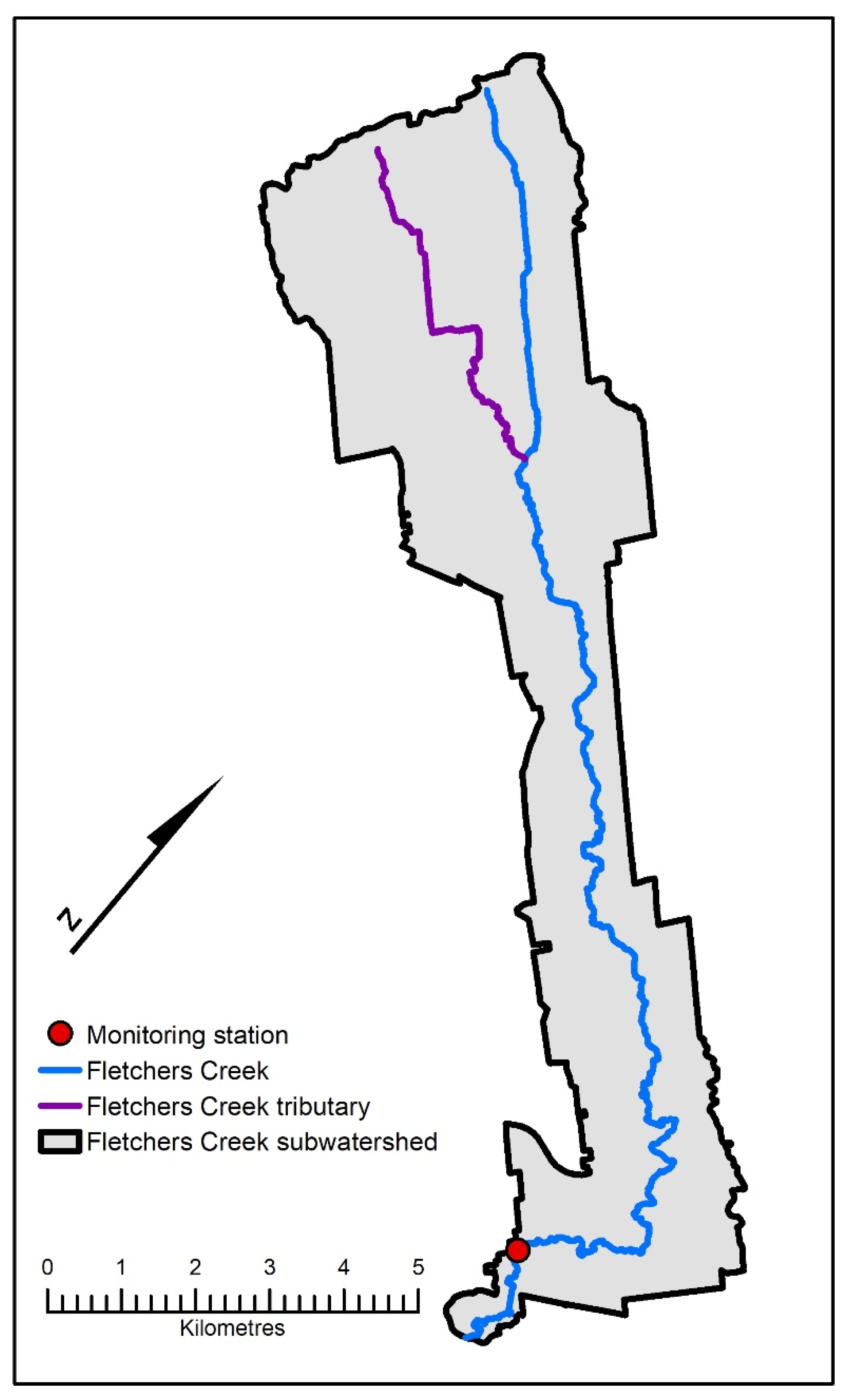
The river network of major streams (shown as green) of Fletchers Creek sub-watershed is represented as links on grid as shown in Figure 3.

3. Model Results

3.1. Water Movement Model

A water movement model was calibrated for the period of 2008 to 2013 and validated for 2014 and 2018.

Table 2. Data Sources for MIKE SHE Model.

Component	Data Type	Description	Range	Units	Reference Source
Topography	Digital Elevation Model	Surface Elevation	264–152	MSL	[40]
Climate	Precipitation Rate	Observed daily Precipitation	0–29.5	mm	[40]
	Reference Evapotranspiration	Calculated based on the FAO guidelines	0.3–6.4	mm	[40]
	Air Temperature	Observed hourly temperature	−29.6–38.1	°C	[40]
	Snow-Melting Temperature	Threshold Melting Temperature	0	°C
	Degree-Day Coefficient	Degree-day Melting or Freezing Coefficient	2	mm/°C/day
	Solar Radiation	Solar Radiation	0–4614	MJ/m2/h	[40]
Land Use	Leaf Area Index	Calibrated, Seasonal, Land Use Distributed	0.2–6	[-]	[40]
	Root Depth	Calibrated, Seasonal, Land Use Distributed	0–3000	mm	[40]
	Kc	Calibrated, Seasonal, Land Use Distributed	0.2–2.2	[-]	[40]
Evapotranspiration	Canopy Interception	Default	0.05	mm
	Soil Evaporation Factor	Default	0.3
	Plant transpiration Factor	Default	0.2
	Water Stress on the Transpiration Process Factor	Default	20	mm/day
	Rot Distribution in the Soil Factor	Default	0.25	/m
Overland Flow	Manning’s M	Calibrated	10	m1/3/s
	Detention Storage	Calibrated, Land Use Distributed	2.5–37.5	m
	OL Drain Depth		0.01	m
	OL Drain Inflow Constant	Default	0.001	/s
	OL Drain Outflow Constant	Calibrated	0.001	/s
	OL Drain Runoff Coefficient	Calibrated, Land Use Distributed	0.012–0.096	[-]
Unsaturated Flow	Hydraulic Conductivity at Saturation Ks	Soil Type Distributed	1.7 × 10−5–1.7 × 10−7	m/s	UNSODA basic soil classes
	Saturated Moisture Content	Soil Type Distributed	0.39–0.51		UNSODA basic soil classes
	Residual Moisture Content	Soil Type Distributed	0.074–0.129		UNSODA basic soil classes
	Alpha	Soil Type Distributed	0.021–0.035	/cm	UNSODA basic soil classes
	N	Soil Type Distributed	1.2–2.39	[-]	UNSODA basic soil classes
	Shape factor	Soil Type Distributed	0.5	[-]	UNSODA basic soil classes
Saturated Zone	Layer Thickness	Distributed	0.5–19.2	m	[40]
	Horizontal Hydraulic Conductivity	Distributed	0–9.6 × 10−3	m/s	[40]
	Vertical Hydraulic Conductivity	Distributed	0–6 × 10−5	m/s	[40]
	Specific Yield	Distributed	0.2–0.3
	Specific Storage	Distributed	1.5 × 10−3–3 × 10−3	/m	[40]
	SZ Drain Depth	Uniform	−0.5	m
	SZ Drain Area	Buffer around the full river network	20	m
	SZ Drain Time Constant	Calibrated	5.6 × 10−7

describes the data sources utilized in this application.

The time steps used for MIKE HYDRO and MIKE SHE are described in Table S3 in Supplementary.

Calibration and Validation Methodology for MIKE SHE and MIKE HYDRO

MIKE SHE and MIKE HYDRO for Fletchers Creek were calibrated and validated using the following statistical parameters: Mean Error (ME), Mean Absolute Error (MAE), Root-Mean-Square-Error (RMSE), Correlation Coefficient (R) and Nash–Sutcliffe model efficiency coefficient (NSE). The hourly model run statistics from the calibration period of 2014–2015 and validation period of 2016 to 2018 are indicated in

Table 3. Statistics of Calibrated and Validated Models.

	Period	ME	MAE	RMSE	R (Correlation)	Nash–Sutcliffe Model Efficiency Coefficient (NSE)
Calibration	January 2014–December 2015	0.066	0.21	0.55	0.68	0.46
Validation	January 2016–December 2018	0.002	0.25	0.56	0.76	0.55

.

3.2. ECO Lab Model Calibration

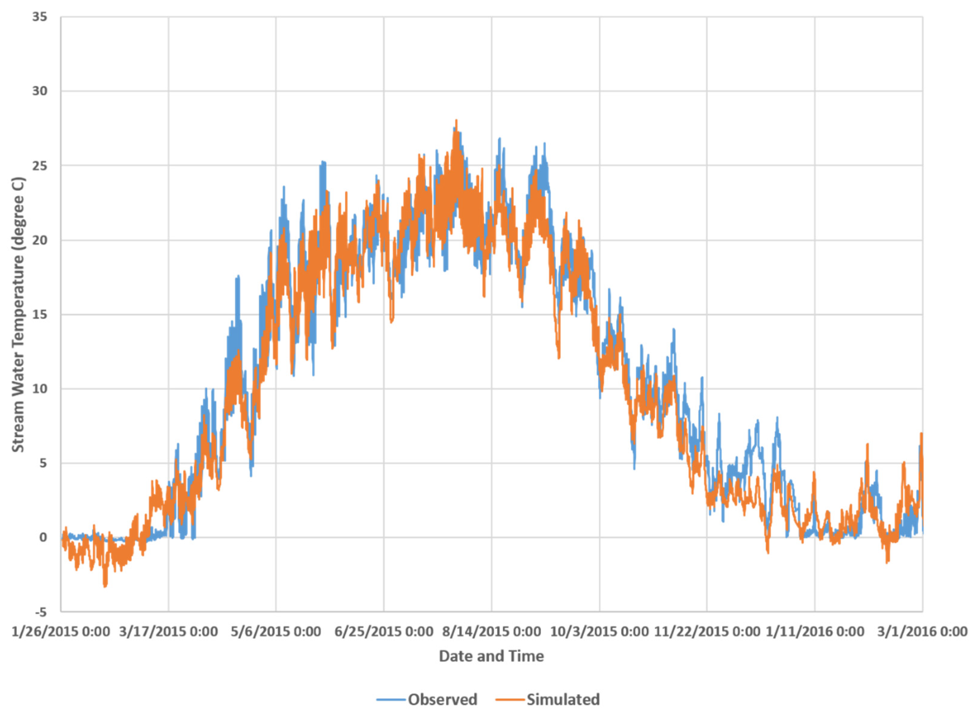
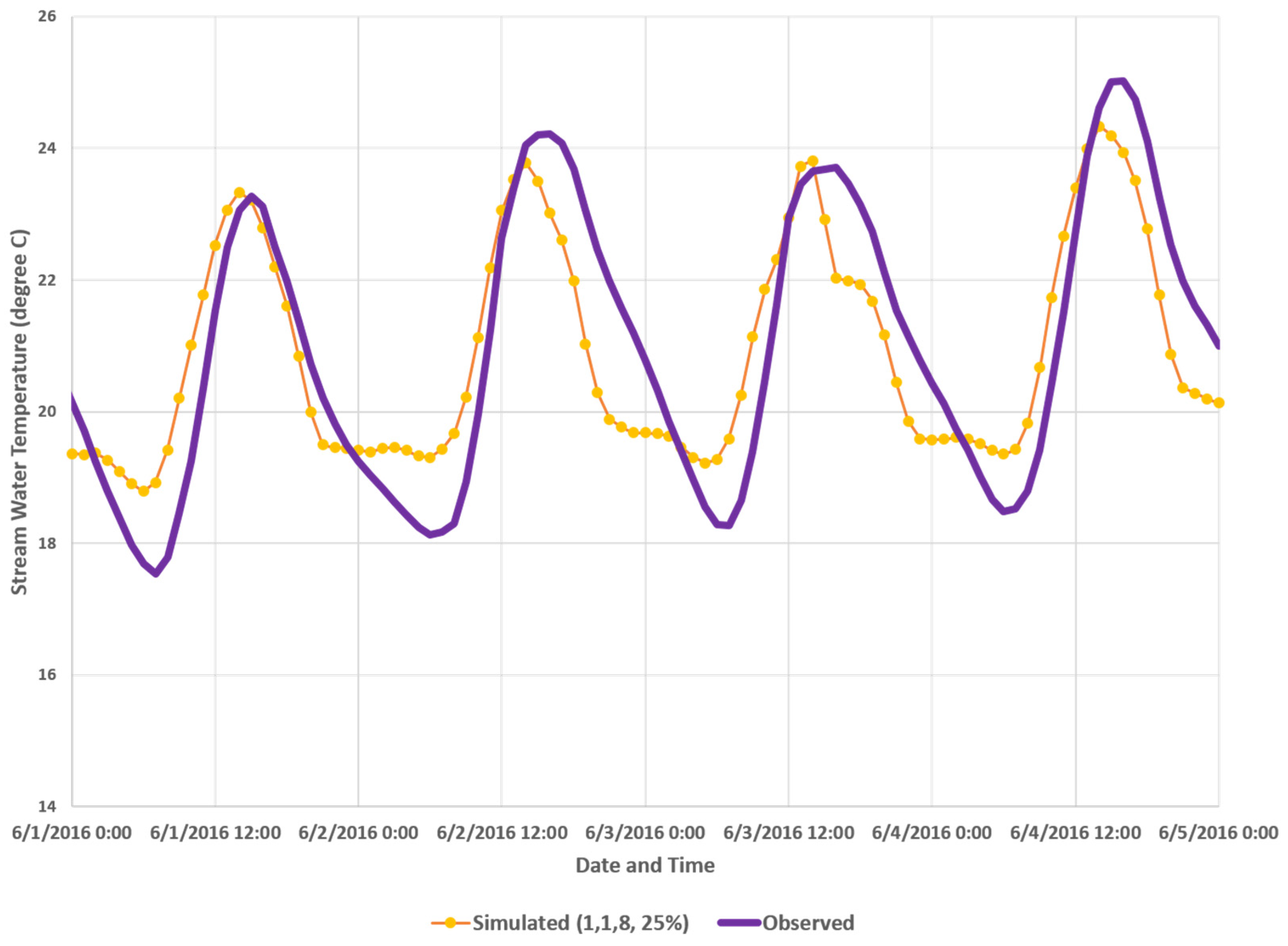
An example of calibration of the ECO Lab model is shown in Figure 4 for two years with observed and simulated stream water temperature for only a single year and in Figure 5 for the simulated and observed stream water temperatures shown for an example of a selected event using four parameters, namely, C1 latent constant (C1_latent), C2 latent constant (C2_latent), Volume Coefficient (Vol Coefficient) and various percentiles of SZ temperature time series. The calibrated parameters of 1, 1, 8 and 25 Percentiles yielded R of 0.96 and NSE of 0.955 for the duration from 27 January 2015 to 30 November 2016 (~2 years).

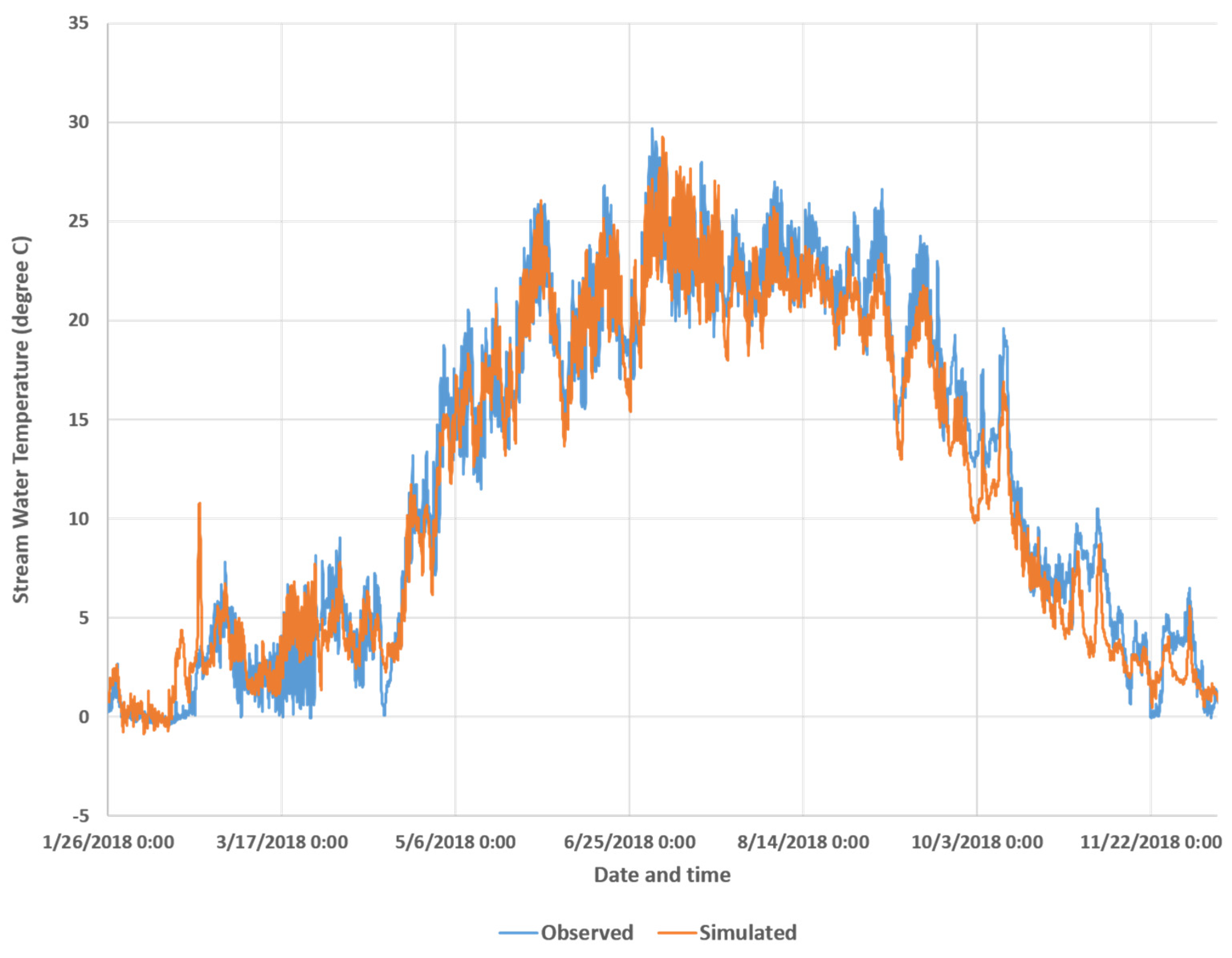
The results from validation of the ECO Lab model are shown in Figure 6 for two years as an example. The calibrated ECO Lab model was validated for the duration from 1 February 2017 to 30 November 2018 (~2 years) with statistical parameters of R of 0.96 and NSE of 0.958. These results indicate that brook trout, with a sustainable temperature range of 10–20 °C, would be impacted and cold-water fish species that are intolerant of water temperatures that exceed 22 °C in summer are in jeopardy, even pre-development conditions [41].

4. Scenario Assessments

4.1. Impact of Land Use Change

Indications of the existing land uses in Fletchers Creek watershed are demonstrated in Figure 7.

Figure 7 shows in the legend that there are land uses of agriculture and barren (no-2 and no-4) in the northern part of the Fletchers Creek sub-watershed. In that area, two land use scenarios are assessed to characterize the implications of land use changes, involving ~8.7% of Fletchers Creek sub-watershed being assessed, i.e., the upper area shown as dark blue and light blue as shown in Figure 7 is changed to (a) Low-Density Urban Land Use Change (Scenario-1) and (b) High-Density Urban Use Change (Scenario-2).

4.1.1. Evaluation of Land Use Change Impacts from Rural to Urban Areas, Scenarios Evaluated Using MIKE Model

For Scenarios-1 and -2, the same calibrated parameters for the Water Movement model and Heat Balance Model were used such as Leaf Area Index, Root Depth, Kc, detention storage, runoff coefficients, cross-sections, river links and thicknesses, horizontal and vertical hydraulic conductivities, specific storage, and safe yields of various aquifers for the water movement model. The same calibrated parameters for the ECO Lab model such as C1, C2, volume coefficients, and groundwater temperature percentile were employed.

4.1.2. Results of Water Balance of Fletchers Creek Watershed Bases with Land Use Change Scenarios

Both Scenarios-1 and -2 are shown for 2016 and 2017 where 2016 was a relatively dry year and 2017 a relatively wet year. Regarding the water movement,

Table 4. Water Balance of No Land Use Change (Existing), Low-Density Urban Land Use Change (Scenario-1) and High-Density Urban Land Use Change (Scenario-2)—Water Movement Model.

	2016—A Relatively Dry Year			2017—A Relatively Wet Year
	No Land Use Change	Scenario-1	Scenario-2	No Land Use Change	Scenario-1	Scenario-2
	Cumulated in mm			Cumulated in mm
Precipitation	608.7	608.7	608.7	791.9	791.9	791.9
Evapotranspiration	448.7	444.4	436.5	435.8	425.5	415.2
OL → River	56.9	78.8	80.7	194.9	202.1	205.9
SZ Drain → River	44.5	51.0	52.5	91.1	92.2	94.8
Base flow to river	57.8	56.7	56.8	73.4	73.5	73.5

shows the changes in various components of water balance in the watershed. There are some changes in overland flow quantities but minimal for base flow and saturated zone drain flows with the change from agriculture to high-density urban land use change.

The results in Table 4 indicate that evapotranspiration decreased from 448.7 mm to 444.4 and 436.5 with Scenario-1 and -2 for both dry and wet years. The overland flow (from 56.9 to 78.8 mm for Scenario-1 and 56.9 to 80.7 for Scenario-2) in a dry year and (from 194.9 to 202.1 mm for Scenario-1 and 194.9 to 205.9 for Scenario-2 in a wet year), and saturated drain flow (44.5 to 52.5 mm) increased more in Scenario-2 and less in Scenario-1.

4.1.3. Results of ECO Lab Model with Land Use Change Scenarios

Using the ECO Lab model, maximum hourly stream water temperature changes at various distances from most the upstream point of Fletchers Creek and Fletchers Creek tributary were analyzed for both scenarios.

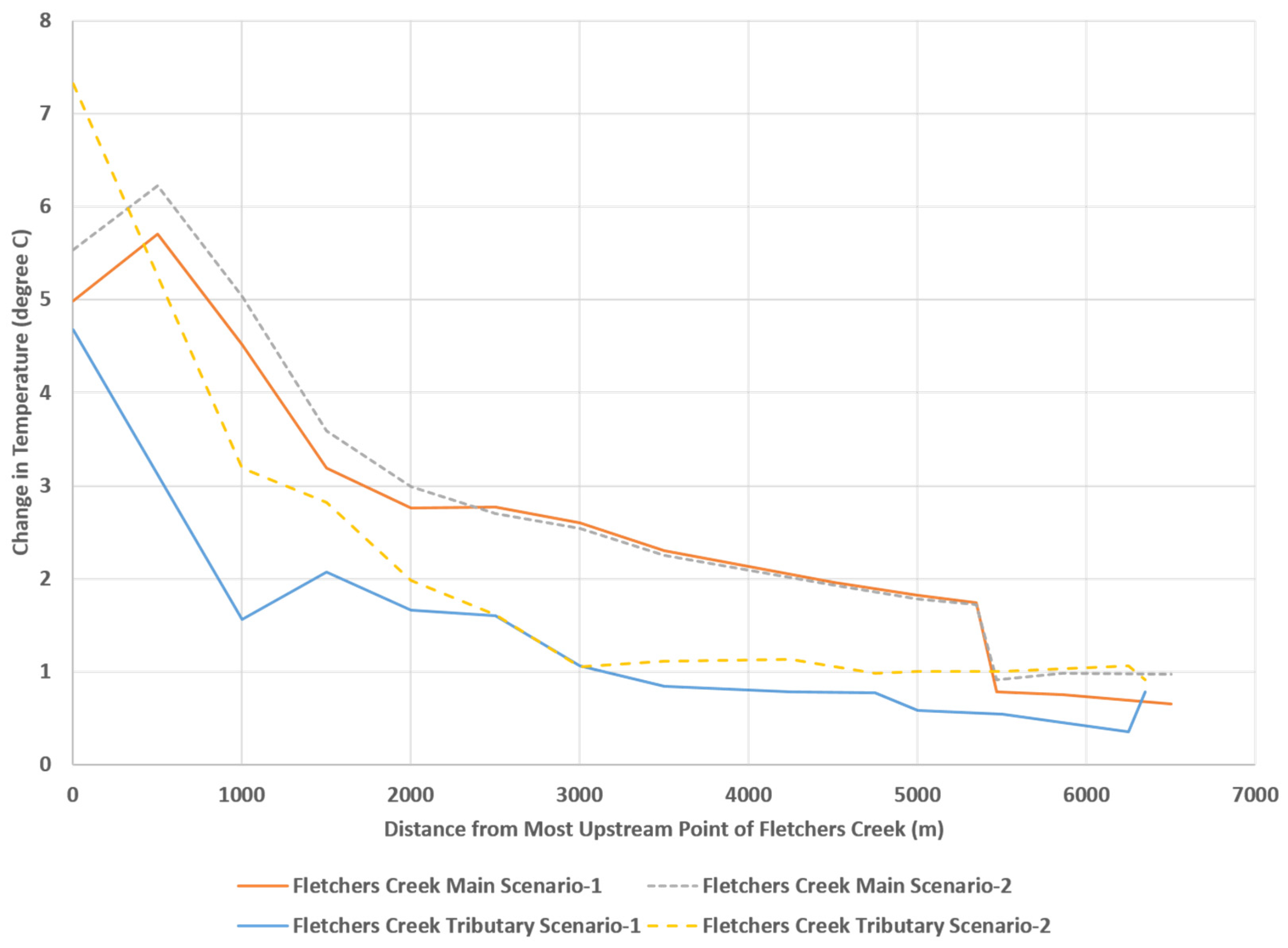
Figure 8 shows that in 2016 (a dry year) for Scenario-1, the maximum hourly stream water temperature is estimated to increase by ~4.8 °C at a 500 m distance from the most upstream point of Fletchers Creek to 3.80 °C at 2000 m distance from the most upstream point of Fletchers Creek, and 0.5 °C at a 6500 m distance from the most upstream point of Fletchers Creek. In Fletchers Creek tributary, as shown in Figure 8, the maximum hourly stream water temperature change increases by 5.92 °C at the origin from the most upstream point of Fletchers Creek tributary to 2.1 °C at a 1000 m distance from the most upstream point of Fletchers Creek and 0.25 °C at a 6000 m distance from the most upstream point of Fletchers Creek tributary.

Figure 8 also shows that in 2016 (a dry year) for Scenario-2, the maximum hourly stream water temperature increases by ~5.4 °C at a 500 m distance from the most upstream point of Fletchers Creek, by 3.6 °C at a 2000 m distance from the most upstream point of Fletchers Creek, by 0.6 °C at a 6500 m distance from the most upstream point of Fletchers Creek. In Fletchers Creek tributary, the maximum hourly stream water temperature is expected to increase by ~6.1 °C at 0 m, by 2.0 °C at a 1000 m distance from the most upstream point of Fletchers Creek and by 0.6 °C at a 6000 m distance from the most upstream point of Fletchers Creek tributary.

Figure 9 shows that in 2017 (a wet year) for Scenario-1, the maximum hourly stream water temperature increases by ~5.7 °C at a 500 m distance, by 2.78 °C at a 2000 m distance from the most upstream point of Fletchers Creek and by 0.66 °C at a 6500 m distance from the most upstream point of Fletchers Creek. In a tributary of Fletchers Creek, the maximum hourly stream water temperature increases by ~4.68 °C at 0 m distance, by 1.67 °C at a 1000 m distance from the most upstream point of Fletchers Creek and by 0.78 °C at 6350 m from the most upstream point of Fletchers Creek tributary.

Figure 9 shows that in 2017 (a wet year), Scenario-2 impacts the maximum hourly stream water temperature increases by ~6.3 °C at a 500 m distance from the most upstream point of Fletchers Creek, by 3.0 °C at a 2000 m distance from the most upstream point of Fletchers Creek and 0.9 °C at a 6500 m distance from the most upstream point of Fletchers Creek. In Fletchers Creek tributary, the maximum hourly stream water temperature increases by almost 7.3 °C at a 0 m distance from the most upstream point of Fletchers Creek tributary, by 3.2 °C at a 1000 m distance from the most upstream point of Fletchers Creek tributary and 0.9 °C at 6350 m from the most upstream point of Fletchers Creek tributary. Monthly maximum hourly stream water temperature change increases are shown in Figures S1–S4.

From the above findings, it is apparent that measurable temperature increases in water temperature occur at ~6500 m downstream due to land use changes.

Duration of the Stream Temperature Increase Due to Land Use Change

Cold-water fish communities are intolerant of water temperatures that exceed 22 °C while some species of salmonids that can tolerate maximum summer temperatures up to 24 °C for brief periods of time [41]. Therefore, analyses carried out for Scenario-2 involved characterization of the number of continuous hours the increases in stream water temperature remained above 1, 2, 3, 4 and 5 °C at various distances from the most upstream point of Fletchers Creek and its tributary. Examples of the results are provided in

Table 5. Number of Continuous Hours the Stream Water Remained Above Various °C at Various Distances.

Location	Increase in Temperature by °C by High Density Land Use Change (Scenario-2) in Fletchers Creek
	1	2	3	4	5
	°C
Fletchers Creek—0	24	11	5	1	1
Fletchers Creek—500	35	13	7	4	1
Fletchers Creek—1000	34	14	7	5	1
Fletchers Creek—1500	25	12	4	0	0
Fletchers Creek—2000	24	7	0	0	0
Fletchers Creek—2500	13	7	0	0	0
Fletchers Creek—3000	11	6	0	0	0
Fletchers Creek—3500	10	3	0	0	0
Fletchers Creek—4500	10	0	0	0	0
Fletchers Creek—5000	9	0	0	0	0
Fletchers Creek—5862	0	0	0	0	0

. The stream water temperature change increase remained continuously above 1 °C for 24, 35, 34, 25 and 24 h at 0, 500, 1000, 1500, 2000 m from the most upstream point of Fletchers Creek. At 5000 m from the most upstream point of Fletchers Creek, the stream water temperature change increased more than 1 °C for nine hours. The stream water temperature change remained continuously above 4 °C for 1, 4, and 5 h continuously at 0, 500, and 1000 m from the most upstream point of Fletchers Creek. In Fletchers Creek tributary, the stream water temperature change increases remained continuously above 1 °C for 49, 32, 18, 14, and 14 h at 0, 1000, 1500, 2000, and 2500 m from the most upstream point of Fletchers Creek’s tributary.

The stream water temperature change remained continuously above 1 °C for 24, 35, 34, 25, and 24 h at 0, 500, 1000, 1500, and 2000 m from the most upstream point of Fletchers Creek. At 5000 m from the most upstream point of Fletchers Creek, the stream water temperature change increased more than 1 °C for 9 h. The stream water temperature remained continuously above a 4 °C increase for 1, 4, and 5 h continuously at 0, 500, and 1000 m from the most upstream point of Fletchers Creek.

Table 5 shows that for 1500 m from the most upstream point of Fletchers Creek, the stream water temperature increase remained above 3 °C from 4 to 7 h. This continuous elevated temperature can destroy spawning habitats and block fish migration, especially for cold-water fish species. Fish such as trout are very temperature-dependent. Cold-water fish species are intolerant of water temperature that exceeds 22 °C in summer. Mixed-water fish species can tolerate water temperature that exceeds 24 °C for brief periods of time.

4.2. Impact of Climate Change

Thermal regimes in streams and rivers are critical to aquatic ecosystems and are anticipated to change as the Earth’s temperature rises due to climate change. To understand how these ecosystems are going to be affected by climate change, it is important have a description and attribution of stream temperature changes [42]. A temperature increase of 10 °C of water will approximately double the rate of physiological function for most fish. Some species can manage this metabolic rate better than others [43].

Riverine ecosystems are particularly vulnerable to climate change because (1) many species within these habitats have limited dispersal abilities as the environment changes, (2) water temperature and availability are climate-dependent, and (3) many systems are already exposed to numerous human-induced pressures [44]. The ecological consequences of future climate changes in freshwater ecosystems will largely depend on the rates and magnitudes of change.

Eleven years of precipitation and air temperature time series were updated by the future climate change RCP 4.5 scenario for 2050 as reported by Region of Peel [45] which provided seasonal mean temperature changes in °C and seasonal mean increases in precipitation. The temperature and precipitation time series of 2016 are assumed as a typical dry year and temperature and precipitation time series of 2017 as a typical wet year. Modified air temperature and precipitation time series for 2016 (a relatively dry year) and modified air temperature and precipitation time series for 2017 (a relatively wet year) are used for the stream temperature change analysis. A water balance analysis was conducted for 2016 and 2017 for MIKE model runs with climate change RCP 4.5 scenarios and are presented in Table S4 in Supplementary.

4.2.1. Results of ECO Lab Model with Climate Change Scenarios

Maximum Hourly Temperature Change in Fletchers Creek with Climate Change RCP 4.5 Scenario

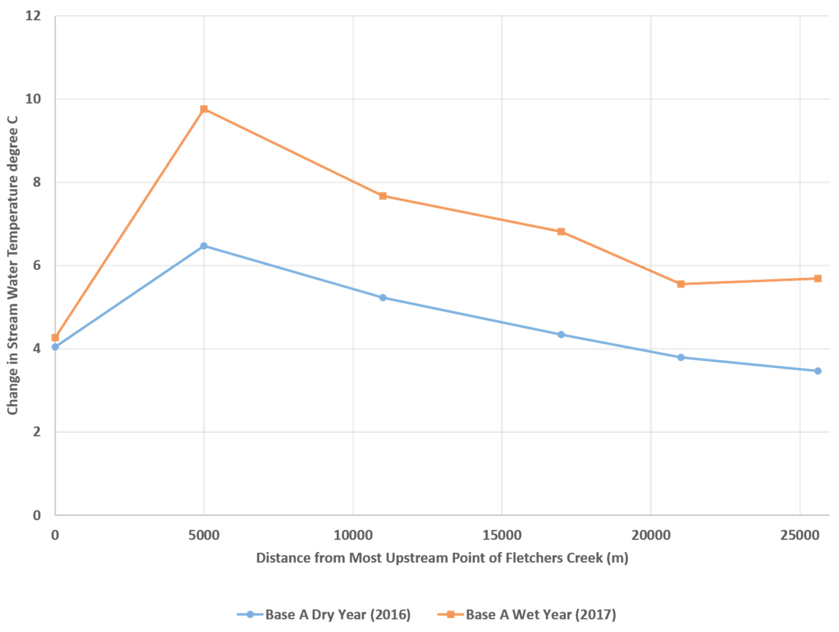
From the results of MIKE model runs, the maximum hourly temperature change in Fletchers Creek with RCP 4.5 Scenario is presented in Figure 10.

With Scenario RCP 4.5, the maximum hourly stream water temperature change in Fletchers Creek is predicted to increase up to 6.5 °C at a distance of 5000 m from the most upstream point and equal to 3.4 °C throughout Fletchers Creek in a typical dry year (Figure 10). As shown in Figure 10, with RCP 4.5, the maximum hourly stream water temperature change in Fletchers Creek can increase up to 9.8 °C for 5000 m and equal 5.7 °C in most of Fletchers Creek in a typical wet year. The total number of hours the Fletchers Creek temperature increases, with climate change RCP 4.5 Scenario in 2050 with Base as a Dry Year—2016 and Base as a Wet Year, are shown in Tables S5 and S6. On a monthly basis, the simulated results are presented in

Table 6. Maximum Monthly Hourly Temperature Change in Fletchers Creek with Climate Change RCP 4.5 Scenario (Typical Dry Year) versus Distance.

Months	Jan	Feb	Mar	Apr	May	Jun	Jul	Aug	Sep	Oct	Nov	Dec	Max
Distance (m)	°C
0	1.3	0.8	4.0	3.1	1.2	0.4	0.2	0.2	0.1	0.2	0.2	0.4	4.0
5000	2.7	5.9	6.2	5.2	6.5	1.7	0.6	0.7	0.7	1.4	4.0	5.8	6.5
11,000	2.4	4.9	5.1	4.9	4.3	1.0	0.7	1.3	0.9	1.2	3.1	5.2	5.2
17,000	2.2	3.3	4.2	4.3	3.9	1.0	1.1	2.2	1.6	0.9	2.3	4.3	4.3
21,000	1.9	2.6	3.5	3.5	2.5	0.8	0.8	1.6	1.0	0.8	1.6	3.8	3.8
25,607	1.7	2.2	3.3	3.1	3.2	0.7	0.7	1.4	1.0	0.7	1.6	3.5	3.5

and

Table 7. Maximum Monthly Hourly Temperature Changes in Fletchers Creek with Climate Change RCP 4.5 Scenario (Typical Wet Year).

Month	Jan	Feb	Mar	Apr	May	Jun	Jul	Aug	Sep	Oct	Nov	Dec	Max
Distance (m)	°C
0	2.3	2.5	3.5	4.3	2.7	4.0	0.3	0.2	0.3	0.2	0.2	0.3	4.3
5000	3.6	4.1	8.2	4.6	9.0	5.9	3.4	7.5	9.8	2.5	3.8	2.8	9.8
11,000	3.5	3.7	6.0	4.4	7.6	5.5	2.1	6.3	7.7	1.9	3.6	2.5	7.7
17,000	2.7	2.9	3.9	3.7	6.8	4.9	2.2	3.6	4.0	1.2	3.0	2.1	6.8
21,000	2.6	2.4	3.7	3.3	5.6	4.3	2.6	2.5	2.8	1.1	2.6	1.9	5.6
25,607	2.5	2.2	3.7	3.1	5.7	4.0	2.3	2.7	2.6	1.2	2.4	1.7	5.7

.

The increase in °C with RCP 4.5 in a dry year at various distances downstream in Fletchers Creek reaches a maximum in February (up to 5.9 °C), March (up to 6.2 °C), April (up to 5.2 °C) and in May (up to 6.5 °C) (Table 6).

Table 7 summarizes the increases in °C with RCP 4.5 in a wet year at various distances downstream in Fletchers Creek, with maxima in March, May, June, August and September.

Duration of the Stream Water Temperature Increases due to Climate Change

The duration of increases (in hours) the stream water temperature remains above a specified °C from the simulated results with RCP 4.5 as this may have an impact on flora and fauna of the stream. The results of these analyses are provided in

Table 8. Number of Continuous Hours the Temperature Increases with Climate Change RCP 4.5 Scenario in 2050 (for Dry Year—2017).

°C	1	2	3	4	5	6	7	8	9
Fletchers Creek at 0	19	8	2	1	0	0	0	0	0
Fletchers Creek at 5000	132	33	13	9	6	3	0	0	0
Fletchers Creek at 11,000	300	56	12	5	2	0	0	0	0
Fletchers Creek at 17,000	176	46	8	4	0	0	0	0	0
Fletchers Creek at 21,000	214	38	9	0	0	0	0	0	0
Fletchers Creek at 25,607	70	26	6	0	0	0	0	0	0

and

Table 9. Number of Continuous Hours of Temperature Increases with Climate Change RCP 4.5 Scenario in 2050 (Base a Wet Year—2017).

°C	1	2	3	4	5	6	7	8	9
Fletchers Creek at 0 m	18	11	7	4	0	0	0	0	0
Fletchers Creek at 5000	41	37	13	9	7	6	5	4	1
Fletchers Creek at 11,000	106	35	25	11	7	4	3	0	0
Fletchers Creek at 17,000	102	36	15	11	6	3	0	0	0
Fletchers Creek at 21,000	121	33	15	10	3	0	0	0	0
Fletchers Creek at 25,607	106	32	16	9	2	0	0	0	0

.

The continuous stream water temperature increases for a dry year (as shown in Table 8) range from 19 to 300 h at various downstream distances of Fletchers Creek above 1 °C, 8 to 56 h at various downstream distances above 2 °C, 2 to 13 h at downstream distances of Fletchers Creek above 3 °C, 1 to 9 h at various downstream distances of Fletchers Creek above 4 °C, and for 3 h above 6 °C at 5000 m downstream.

As shown in Table 8, with climate change, the continuous number of hours the stream water temperature remains elevated for more than 3 °C (from 5000 m to 25,607 m from the most upstream point of Fletchers Creek) for distances of 20,000 m for more than 6 h and for a distance of 6000 m for more than 12 h. This elevation in temperature may have serious implications for flora and fauna in the creek especially the cold-water and mixed-water fish species.

The continuous stream water temperature change increase for a wet year (as shown in Table 9) ranges from 18 to 121 h at various downstream distances of Fletchers Creek above 1 °C, 11–32 h at various downstream distances of Fletchers Creek above 2 °C, 7–25 h at various downstream distances of Fletchers Creek above 3 °C, 4–11 h at various downstream distances above 4 °C and 5 h above 7 °C at 5000 m downstream in Fletchers Creek.

As shown in Table 9, with climate change the continuous number of hours the stream water temperature remains elevated at more than 3 °C (from 5000 m to 25,607 m from the most upstream point of Fletchers creek) for 20,000 m is more than 13 h. This elevation in temperature may have serious implications for flora and fauna in the creek especially for the cold-water and mixed-water fish species. Cold-water fish such as trout and salmon, which are economically and recreationally valuable, are having their populations constrained by the rising water temperatures. For these fish species, there will be a net loss of habitat as the effects of climate change continue.

5. Summary on Scenario Assessments

These types of analyses can warn the creek manager to assess whether the flora and fauna can bear the shock of increases in stream water temperature. The analyses show that the duration of temperature increases from threshold levels are sufficient to impact the flora and fauna of the stream as examined using modeling results indicating that urbanization may change stream water temperatures for 9% of the time by 1 °C, and 2% of the time by 2 °C for distances of 1000 m downstream. This is as a result of land use change from agriculture to low-density urbanization (e.g., as apparent in [46]) where brook trout have a sustainable temperature range of only 10–20 °C and will be more severely impacted by the effects of both urbanization and climate change, as a result of the temperatures being elevated as calculated. Furthermore, water temperatures in the river change for 20% of the time by 1 °C, and 4% of the time by 2 °C at distances of 1000 m downstream with land use change to high urban development from agriculture. Assessment of climate change impacts for a typical dry year indicates the stream water temperature for 9% of the time will increase between 1 °C and 2 °C, and 2% of the time between 2 °C and 3 °C at distances of 17,000 m downstream with RCP 4.5 Scenario in 2050. Populations of many economically and recreationally valuable cold-water fish such as trout and salmon are already constrained by unsuitably warm temperatures. Net losses of habitat may occur with further warming, and the spatial and temporal impacts are certainly indicative of potential incremental impacts to aquatic life.

As reported by [47,48,49,50], these findings indicate there will be losses of habitat for trout and salmon due to the elevated temperatures from the combination of urbanization and climate change. As found in this research, MIKE models provide an excellent opportunity to spatially and dynamically integrate watershed and heat balance models to assess the impacts of various land use changes and climate change.

6. Conclusions

The conclusions of this research are:

(1)

Overall, the MIKE model combination was able to analyze the impacts of river regime contributions, for both changes in land use and in climate;

(2)

The integration of a physics-based hydraulic model (MIKE SHE) with MIKE HYDRO and ECO Lab was able to simulate stream flows and diurnal summer temperature variations in a case study;

(3)

The combination of models being able to predict the effects of different urbanization scenarios on water temperatures within an appropriate uncertainty framework in the streams was demonstrated, indicating the methods, pathways and a roadmap for conditions that can be expected;

(4)

Prediction of the effects of various climate change scenarios on stream water temperatures provide important insights into the spatial and temporal extent of impacts likely to occur in response to RCP 4.5;

(5)

With the delineation of the impacts of urbanization and climate change on temperatures, concerns with the spatial impacts of urbanization and climate change on portions of the Credit River warrant assessment as to the degree to which these impacts will influence aquatic life, suggesting that options for shading, etc., may be warranted for protection.

References

- Carrivick, J.L.; Brown, L.E.; Hannah, D.M.; Turner, A.G.D. Numerical modelling of spatio-temporal thermal heterogeneity in a complex river system. J. Hydrol. 2012, 414, 491–502. [Google Scholar] [CrossRef] [Green Version]
- Elmore, L.R.; Null, S.E.; Mouzon, N.R. Effects of Environmental Water Transfers on Stream Temperatures. River Res. Appl. 2015, 32, 1415–1427. [Google Scholar] [CrossRef] [Green Version]
- Fabris, L.; Malcolm, I.A.; Buddendorf, W.B.; Soulsby, C. Integrating process-based flow and temperature models to assess riparian forests and temperature amelioration in salmon streams. Hydrol. Processes 2018, 32, 776–791. [Google Scholar] [CrossRef]
- McBean, E.A.; Burn, D.H. Thermal Modeling in Urban Runoff and the Implications to Stormwater Pond Design. Presented at International Symposium on Urban Hydrology, Hydraulics and Sediment Control, Lexington, KY, USA, 25–28 July 1983; University of Kentucky: Lexington, KY, USA, 1983. [Google Scholar]
- Jones, M.P.; Hunt, W.F.; Winston, R.J. Effect of urban catchment composition on runoff temperature. J. Environ. Eng. 2012, 138, 1231–1236. [Google Scholar] [CrossRef]
- Hester, E.T.; Bauman, K.S. Stream and retention pond thermal response to heated summer Runoff from urban impervious surfaces. J. Am. Water Resour. Assoc. 2013, 49, 328–342. [Google Scholar] [CrossRef]
- Guzy, M.; Richardson, K.; Lambrinos, J.G. A tool for assisting municipalities in developing riparian shade inventories. Urban For. Urban Green. 2015, 14, 345–353. [Google Scholar] [CrossRef]
- Fabris, L.; Malcolm, I.A.; Buddendorf, W.B.; Millidine, K.J.; Tetzlaff, D.; Soulsby, C. Hydraulic modelling of the spatial and temporal variability in Atlantic salmon parr habitat availability in an upland stream. Sci. Total Environ. 2017, 601, 1046–1059. [Google Scholar] [CrossRef]
- Caldwell, P.; Segura, C.; Gull Laird, S.; Sun, G.; McNulty, S.G.; Sandercock, M.; Vose, J.M. Short-term stream water temperature observations permit rapid assessment of potential climate change impacts. Hydrol. Processes 2015, 29, 2196–2211. [Google Scholar] [CrossRef]
- Hannah, D.M.; Garner, G. River water temperature in the United Kingdom: Changes over the 20th century and possible changes over the 21st century. Prog. Phys. Geogr. 2015, 39, 68–92. [Google Scholar] [CrossRef] [Green Version]
- Michel, A.; Schaefli, B.; Wever, N.; Zekollari, H.; Lehning, M.; Huwald, H. Future water temperature of rivers in Switzerland under climate change investigated with physics-based models. Hydrol. Earth Syst. Sci. Discuss. 2021; in review. [Google Scholar] [CrossRef]
- Chen, H.; Huang, J.; McBean, E.; Singh, V. Evaluation of Alternative Two-Source Remote Sensing Models in Partitioning of Land Evapotranspiration. J. Hydrol. 2021, 597, 126029. [Google Scholar] [CrossRef]
- Deas, M.L.; Lowney, C.L. Water Temperature Modeling Review; Central Valley, Bay Delta Modeling Forum: Vacaville, CA, USA, 2000; p. 113. [Google Scholar]
- Caissie, D. The thermal regime of rivers: A review. Freshw. Biol. 2006, 51, 1389–1406. [Google Scholar] [CrossRef]
- Dugdale, J.; Hannah, D.M.; Malcolm, I.A. River temperature modelling: A review of process-based approaches and future directions, Earth. Earth-Sci. Rev. 2017, 175, 97–113. [Google Scholar] [CrossRef]
- Zhu, S.; Heddam, S.; Nyarko, E.K.; Hadzima-Nyarko, M.; Piccolroaz, S.; Wu, S. Modeling daily water temperature for rivers: Comparison between adaptive neuro-fuzzy inference systems and artificial neural networks models. Environ. Sci. Pollut. Res. 2019, 26, 402–420. [Google Scholar] [CrossRef] [PubMed]
- Islam, S.U.; Hay, R.W.; Déry, S.J.; Booth, B.P. Modelling the impacts of climate change on riverine thermal regimes in western Canada’s largest Pacifc watershed. Sci. Rep. 2019, 9, 11398. [Google Scholar] [CrossRef]
- Toffolon, M.; Piccolroaz, S. A hybrid model for river water temperature as a function of air temperature and discharge. Environ. Res. Lett. 2015, 10, 11. [Google Scholar] [CrossRef]
- DHI. MIKE SHE, Volume 1: User Guide, MIKE 2017; Agern Allé 5 2970: Hørsholm, Denmark, 2017. [Google Scholar]
- DHI. MIKE 11, A Modelling System for Rivers and Channels, MIKE 11, Reference Manual, MIKE 2017; Agern Allé 5 2970: Hørsholm, Denmark, 2017. [Google Scholar]
- DHI. MIKE ECO Lab, Numerical Lab for Ecological and Agent Based Modelling, User Guide, MIKE 2017; Agern Allé 5 2970: Hørsholm, Denmark, 2017. [Google Scholar]
- Ouellet, V.; Secretan, Y.; St-Hilaire, A.; Morin, J. Daily averaged 2D water temperature model for the St. Lawrence River. River Res. Appl. 2014, 30, 733–744. [Google Scholar] [CrossRef]
- Refsgaard, J.; Storm, B. MIKE SHE. In Computer Models of Watershed Hydrology; Singh, V., Ed.; Water Resources Publications: Englewood, CO, USA, 1995; pp. 809–846. [Google Scholar]
- Thompson, J.R.; Sørenson, H.R.; Gavin, H.; Refsgaard, A. Application of the coupled MIKE SHE/MIKE 11 modelling system to a lowland wet grassland in southeast England. J. Hydrol. 2004, 293, 151–179. [Google Scholar] [CrossRef]
- Butts, M.; Loinaz, M.C.; Bauer-Gottwein, P.; Blasone, R.; Von Christierson, B.; Hansen, F.T.; Jensen, J.K.; Poulsen, J.B. Eco-hydrological process simulations within an integrated surface water-groundwater model. In Proceedings of the 11th International Conference on Hydroinformatics, New York, NY, USA, 17–21 August 2014. [Google Scholar]
- House, M.C.; Thompson, A.R.; Sorensen, J.; Roberts, P.R.; Acreman, M.C. Modelling groundwater/surface water interaction in a managed riparian chalk valley wetland, Hydrological Processes. Hydrol. Processes 2016, 30, 447–462. [Google Scholar] [CrossRef] [Green Version]
- Andersen, J.; Refsgaard, J.C.; Jensen, K.H. Distributed hydrological modelling of the Senegal River Basin—Model construction and validation. J. Hydrol. 2001, 247, 200–214. [Google Scholar] [CrossRef]
- Stisen, S.; Jensen, K.H.; Sandholt, I.; Grimes, D.I. A remote sensing driven distributed hydrological model of the Senegal River basin. J. Hydrol. 2008, 354, 131–148. [Google Scholar] [CrossRef]
- Feyen, L.; Vázquez, R.; Christiaens, K.; Sels, O.; Feyen, J. Application of a distributed physically-based hydrological model to a medium size catchment. Hydrol. Earth Syst. Sci. Discuss. 2000, 4, 47–63. [Google Scholar] [CrossRef]
- Huang, Y.; Chen, X.; Li, Y.; Willems, P.; Liu, T. Integrated modeling system for water resources management of Tarim River Basin. Environ. Eng. Sci. 2010, 27, 255–269. [Google Scholar] [CrossRef]
- Singh, C.R.; Thompson, J.R.; Kingston, D.G.; French, J.R. Modelling water-level options for ecosystem services and assessment of climate change: Loktak Lake, northeast India. Special issue: Ecosystem Services of Wetlands. Hydrol. Sci. J.—J. Sci. Hydrol. 2011, 56, 2011. [Google Scholar]
- Wang, S.; Zhang, Z.; Sun, G.; Strauss, P.; Guo, J.; Tang, Y.; Yao, A. Multi-Site Calibration, Validation, and Sensitivity Analysis of the MIKE SHE Model for a Large Watershed in Northern China. Hydrol. Earth Syst. Sci. 2012, 16, 4621–4632. Available online: www.hydrol-earth-syst-sci.net/16/4621/2012/doi:10.5194/hess-16-4621-2012 (accessed on 17 July 2020). [CrossRef] [Green Version]
- Refsgaard, J.C.; Sørensen, H.R.; Mucha, I.; Rodak, D.; Hlavaty, Z.; Bansky, L.; Klucovska, J.; Topolska, J.; Takáč, J.; Kosc, V.; et al. An Integrated Model for the Danubian Lowland—Methodology and Applications. Water Resour. Manag. 1998, 12, 433–465. [Google Scholar] [CrossRef]
- Al-Khudhairy, D.H.A.; Thompson, J.R.; Gavin, H.; Hamm, N.A.S. Hydrological modelling of a drained grazing marsh under agricultural land use and the simulation of restoration management scenarios. Hydrol. Sci. J. 1999, 44, 943–971. [Google Scholar] [CrossRef]
- Thompson, J.R.; Laizé, C.L.R.; Green, A.J.; Acreman, M.C.; Kingston, D.G. Climate change uncertainty in environmental flows for the Mekong River. Special issue: Hydrological Science for Environmental Flows. Hydrol. Sci. J.—J. Sci. Hydrol. 2014, 59, 935–954. [Google Scholar] [CrossRef] [Green Version]
- Thompson, J.R.; Green, A.J.; Kingston, D.G. Potential evapotranspiration-related uncertainty in climate change impacts on river flow: An assessment for the Mekong River basin. J. Hydrol. 2014, 510, 259–279. [Google Scholar] [CrossRef] [Green Version]
- CVC. Fletchers Creek Restoration Study, Appendix 1, Characterization Report; Credit Valley Conservation: Mississauga, ON, Canada, 2012. [Google Scholar]
- CVC; (Credit Valley Conservation: Mississauga, ON, Canada). Personal Communication, 2020.
- CVC; (Credit Valley Conservation: Mississauga, ON, Canada). Personal Communication, 2021.
- CVC; (Credit Valley Conservation: Mississauga, ON, Canada). Personal Communication, 2019.
- CVC. A Cooperative Management Planning Initiative for the Credit River Fishery; Ministry of Natural Resources; Credit Valley Conservation: Mississauga, ON, Canada, 2002. [Google Scholar]
- Wright, J.; Imhof, J. Technical Background Report for the Grand River Fisheries Management Plan; Report to Grand River Conservation Authority and Ontario Ministry of Natural Resources: Cambridge, ON, Canada, 2001. [Google Scholar]
- Bennett, W.A.; Di Santo, V. Effect of rapid temperature change on resting routine metabolic rates of two benthic elasmobranchs. Fish Physiol. Biochem. 2011, 37, 929–934. [Google Scholar]
- Woodward, G.; Perkins, D.M.; Brown, L.E. Climate change and freshwater ecosystems: Impacts across multiple levels of organization. Philos. Trans. R. Soc. B Biol. Sci. 2010, 365, 2093–2106. [Google Scholar] [CrossRef] [Green Version]
- Auld, H.; Switzman, H.; Comer, N.; Eng, S.; Hazen, S.; Milner, G. Region of Peel. Climate Trends and Future Projections in Region of Peel, Technical Report; Ontario Climate Consortium: Toronto, ON, Canada, 2016. [Google Scholar]
- Mohseni, O.; Stefan, H.G.; Eaton, J.G. Global warming and potential changes in fish habitat in U.S. streams. Clim. Chang. 2003, 59, 389–409. [Google Scholar] [CrossRef]
- Isaak, D.J.; Wollrab, S.; Horan, D.; Chandler, G. Climate change effects on stream and river temperatures across the northwest U.S. from 1980–2009 and implications for salmonid fishes. Clim. Chang. 2012, 113, 499–524. [Google Scholar] [CrossRef] [Green Version]
- Rieman, B.E.; Isaak, D.J.; Adams, S.; Horan, D.; Nagel, D.; Luce, C.; Myers, D. Anticipated climate warming effects on bull trout habitats and populations across the Interior Columbia River Basin. Trans. Am. Fish Soc. 2007, 136, 1552–1565. [Google Scholar] [CrossRef]
- Isaak, D.J.; Luce, C.H.; Rieman, B.E.; Nagel, D.E.; Peterson, E.E.; Horan, D.L.; Parkes, S.; Chandler, G.L. Effects of climate change and recent wildfires on stream temperature and thermal habitat for two salmonids in a mountain river network. Ecol. Appl. 2010, 20, 1350–1371. [Google Scholar] [CrossRef] [PubMed] [Green Version]
- Wenger, S.J.; Isaak, D.J.; Luce, C.H.; Neville, H.M.; Fausch, K.D.; Dunham, J.D.; Dauwalter, D.C.; Young, M.K.; Elsner, M.M.; Rieman, B.E.; et al. Flow regime, temperature, and biotic interactions drive differential declines of trout species under climate change. Proc. Natl. Acad. Sci. USA 2011, 108, 14175–14180. [Google Scholar] [CrossRef] [PubMed] [Green Version]
Figure 1.
Delineation of Credit River Watershed, Including Fletchers Creek Sub-watershed.
Figure 2.
Topography and Hydrologic Network of Fletchers Creek Sub-Watershed.
Figure 3.
Major Streams in Fletchers Creek.
Figure 4.
Observed and Simulated Stream Water Temperature for 2015.
Figure 5.
Observed and Simulated Stream Water Temperature for an Event in 2016.
Figure 6.
Validation Results of Simulated Stream Water Temperature for 2018 year.
Figure 7.
Existing Land Use of Fletchers Creek Sub-watershed. Note: Land use referred to various codes are provided in Table 1 above.
Figure 8.
Maximum Hourly Temperature Changes in Fletchers Creek with Land Use Change from Existing to Low-Density Urban Land Use Change (Scenario-1) with High-Density Urban Land Use Change (Scenario-2) in 2016.