
Identification of High-Impact Uncertainty Sources for Urban Flood Models in Hillside Peri-Urban Catchments


1
Institute of Urban Water Management and Landscape Water Engineering, Graz University of Technology, 8010 Graz, Austria
2
Institute of Hydraulic Engineering and Water Resources Management, Graz University of Technology, 8010 Graz, Austria
*
Author to whom correspondence should be addressed.
Water 2022, 14(12), 1973; https://doi.org/10.3390/w14121973
Submission received: 13 May 2022
/
Revised: 14 June 2022
/
Accepted: 17 June 2022
/
Published: 20 June 2022
(This article belongs to the Section Urban Water Management)
Abstract
:Climate change, as well as increasing urbanization, lead to an increase in urban flooding events around the world. Accurate urban flood models are an established tool to predict flooding areas in urban as well as peri-urban catchments, to derive suitable measures to increase resilience against urban flooding. The high computational cost and complex processes of urban flooding with numerous subprocesses are the reason why many studies ignore the discussion of model uncertainties as well as model calibration and validation. In addition, the influence of steep surface (hillside) conditions on calibration parameters such as surface roughness are frequently left out of consideration. This study applies a variance-based approach to analyze the impact of three uncertainty sources on the two variables—flow and water depth—in a steep peri-urban catchment: (i) impact of DEM validation; (ii) calibration of the model parameter; (iii) differences between 1D/2D and 2D models. The results demonstrate the importance of optimizing sensitive model parameters, especially surface roughness, in steep catchments. Additional findings of this work indicate that the sewer system cannot be disregarded in the context of urban flood modeling. Further research with real heavy storm events is to be pursued to confirm the main results of this study.
1. Introduction
Heavy storm events have increased and will continue to increase in the future in both frequency and amplitude due to climate change [1,2,3,4]. This leads to adverse impacts on human and environmental systems, such as floods [5]. Urbanization as a socio-economic impact of urban population growth represents one main driver in the urban flooding context. Together with global climate change, it is one of the primary sources of increasing flood events [6,7], caused by the associated increase in the impervious surface area [3,8,9]. Numerous documented events worldwide in past years confirm the threat posed to society by urban floods (e.g., Ljubljana 2021 (Slovenia), Kufstein 2021 (Austria), North Rhine-Westphalia 2021 (Germany), Ankara 2020 (Turkey), Venice 2019 (Italy), Elblag 2017 (Poland), and Wallingford 2014 (UK) [10]).
Based on the observation of air temperature increase induced by climate change, a trend towards extreme storm events [11,12,13] and subsequent flooding can be expected in the future. The reason for this has been highlighted in several studies, which predict an increase of 7 percent in atmospheric water volume per degree of global warming based on the Clausius–Claperyron equation [13,14,15]. This is especially noticeable in the change of extreme storm events [16,17,18]. In urban catchments, flooding is a complex process that is difficult to describe. The increased damage potential is a result of the high building density [19], the often-occurring combination of fluvial and pluvial flooding and the high spatial and temporal variability of extreme storm events [17,20,21]. Additionally, several not-predictable conditions such as blockage scenarios in sewers, streams, or culverts can also have a significant impact on the flooding process [22]. Especially in peri-urban or hilly catchments, which are often characterized by small urban streams, sediment transport-induced blockages of drainage systems can be a likely cause of flooding. These will occur more frequently due to the increase of extreme storm events by climate change and the land cover changes by urbanization [23]. For this reason, urban flooding events are not simply of pluvial or fluvial type but can be defined as a stand-alone type of flooding, which is often a combination of several types [24].
Urban flood models estimating water depth and flow velocity are widely used and accepted tools among researchers and professional engineers [25,26,27]. Types of such flood models span simple and traditional 1D urban drainage models [28], hydrodynamic 2D flood models such as BASEMENT2D [29], raster-based 2D flood models such as CADDIES [30,31], and coupled model approaches, demonstrated by numerous studies [32,33,34,35,36,37].
The required level of model accuracy is one of the most discussed topics in the field of urban flooding. Despite numerous studies published in recent years, there is no clear answer to the question whether the urban drainage system must be included in an urban flood model [38,39,40], if it can be discarded or simplified with source and sink terms [41,42,43]. However, a trend in literature can be identified, leaning towards considering drainage systems in urban flood assessment [44]. While the focus of the past decade was on building a model with the highest accuracy, the current focus is on model application, such as real-time prediction [45,46,47] or the quantification of model uncertainties, sensitivities and calibration techniques [48]. However, model calibration in particular remains a challenge due to the spatially and temporally distributed properties of flooding and the often-poor data basis in terms of measurements [21,49].
A model is always a simplified representation of a real system and can therefore never be without error, which results in the necessity of communicating of model uncertainties [27,50]. Additionally, model complexity is directly related to data availability and consequently to model uncertainty [51,52].
The first step of uncertainty analysis is the identification of the main uncertainty source. This simplifies the quantification of model uncertainties in the workflow as the second step [27,53,54].
In general, four sources of uncertainty should be distinguished in environmental modeling: (i) input data; (ii) model parameters; (iii) model structure; (iv) observational data [54,55].
One key source regarding input data uncertainty is the digital elevation model (DEM), as it significantly impacts the spatial model discretization (2D mesh) of the surface runoff process [43]. If the DEM and the 2D mesh are available in a suitable resolution, the calibration of the sensitive model parameters is one further option to reduce the model uncertainties [56].
The surface roughness parameter particularly depends on the land cover and the surface slope described by the sheet flow condition [57,58]. This must be considered especially in urban hillside catchments where higher surface slopes dominate. The steep surface also influences further model parameters, such as the depression storage [59,60,61] and the hydraulic capacity of rainwater manholes on the streets [62,63]. Therefore, model parameters in hillside catchments must be selected in different ways than in flat urban catchments.
The uncertainties of model structures include the basic model approach (black box, grey box, white box) [64], the relevant processes (e.g., hydrological or hydraulic) [50] and the accurate mathematical description as well as the required boundary conditions [65].
The uncertainties of observations include a wide spectrum [66], from measured input data (e.g., precipitation data) to measured time series used for calibration, such as flow measurements [65]. The lack of measured calibration data often results in an alternative way based on damage data and field observations (e.g., photo and video documentation from social media) to qualitatively validate urban flood models [49,67,68]. Damage data itself introduces uncertainties, for instance resulting from the visual estimation of a selected model variable (e.g., water depth).
While there are numerous studies on flooding in flat urban and peri-urban catchments (e.g., [43,69,70,71,72]), sites with a hillside characteristic are rarely analyzed. Such catchments are often located on the border area of urban catchments. To bridge this gap, a flood model in a hillside peri-urban study site in Graz, Austria was developed in this work. To build up the model, two DEM in different qualities were used to address the impact of the main input data. The differences in slope inclination will influence the selections of model parameters and consequently the calibration and validation of the model. Additionally, two different model structures (with (1D/2D) and without sewer system (1D)) were generated to quantify the impact of the sewer system. These three main uncertainty sources (input data, model parameters, model structure) are analyzed with a variance-based method to identify the uncertainty source with the highest impact, to further the understanding of uncertainties of urban flood modeling, particularly peri-urban hillside catchments.
2. Materials and Methods
A state-of-the-art modeling framework was used to build the urban flood model [73] for the study site. We followed the three major steps in terms of modeling: (i) planning and preparation; (ii) model formulation; (iii) model build, model validation) [74].
The main study objective (planning and preparation) is to identify the most impactful uncertainty source within an urban flooding model. The dominant processes for urban flooding are hydrological runoff generation, the spatial and temporal distribution of surface water flow, flow in a potential urban stream and interaction with the sewer system in form of possible flooding in the urban drainage system [75]. This resulted in a 1D/2D urban flood model with three main model layers: (i) a fully distributed rainfall-runoff model; (ii) a fully distributed 2D surface runoff model (urban surface and urban stream); (iii) a hydrodynamical 1D sewer model. Calibration and validation of the model is based on surface flow and water depth at two monitoring sites and documentation from the sewer operator, fire department and interviews with affected persons. Based on this structure, an urban flood model was built for the hillside study site.
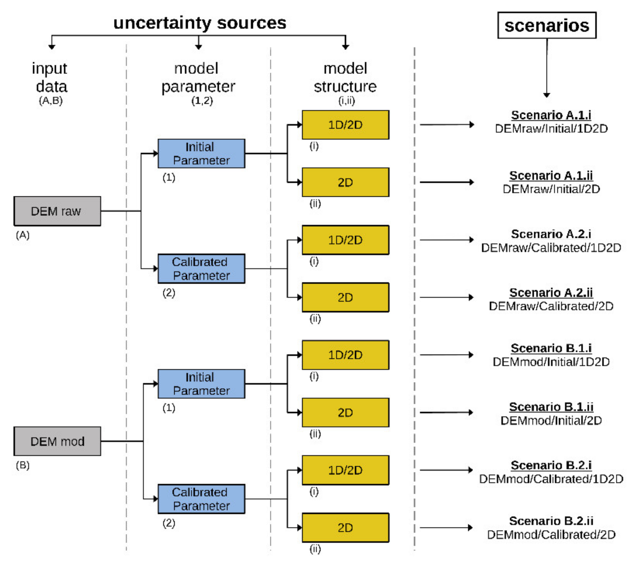
Three main uncertainty sources (n) are analyzed in this study and each of them has two options (k) which resulted in eight different scenarios (nk) (Figure 1). Two available digital elevation models (DEM) represent the main input data to create the urban flood model. The first one represents the original DEM (DEMraw) and the second will be modified with obstructions (DEMmod) as demonstrated by [43]. Furthermore, the spatial resolution of the DEMraw is 1 × 1 m and is lower than that of the DEMmod with 0.4 × 0.4 m.
Based on a comprehensive literature review the initial value of the sensitive model parameters were selected. Liu et al. [48] identified the surface roughness, the hydrological losses such as interception and the infiltration capacity as the key parameters in terms of urban flood modeling. These parameters were calibrated for the steep surface areas to quantify the influence of a high surface slope. This resulted in two different model scenarios with initial literature values for the sensitive model parameters and calibrated values for steep surface conditions. The last analyzed uncertainty source represents two different model structures to identify the impact of the sewer system. Therefore, a coupled 1D/2D model with the sewer system and secondly a 2D model without the sewer system were selected. Precipitation data of two heavy storm events are available for the catchment. One event was used to calibrate the basic model and the other to demonstrate the analysis regarding the identifications of the highest-impact uncertainty sources.
2.1. Study Site Annabach
A small study site in Graz, the capital of Styria, a southern province of Austria, with a total catchment area of 132 hectares was selected. Graz is located on the southern outskirts of the alps and is influenced by Alpine and Mediterranean climate and can be classified as a humid continental climate [76]. The local climate is also influenced by alpine conditions with cold winters and warm summers. Average precipitation per year is 860 mm and the majority of storms can be classified as convective summer storms [20].
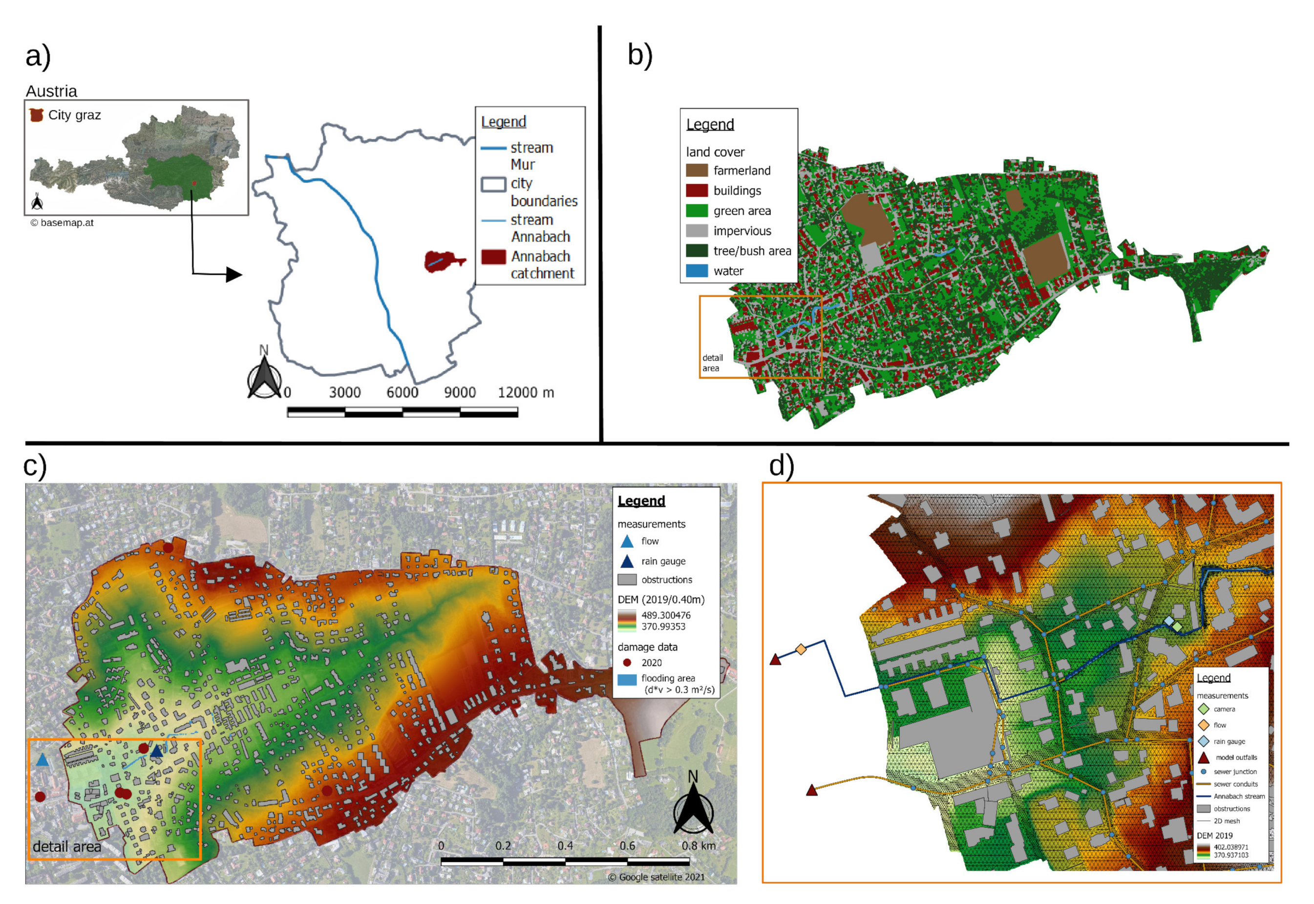
The Annabach catchment can be described as a small peri-urban valley on the outskirts of Graz, with two hillsides to the north (average slope about 10 degrees) and the south (average slope of about 15 degrees) (Figure 2). The catchment is predominantly serviced by a combined sewer system, with the selection of a few sub-catchments serviced with a separate sewer system. Therefore, the urban drainage system considers only the combined and the stormwater sewers. The catchment also includes a small urban stream with a base flow between 5 and 10 L per second. Due to the urban character of the catchment, the stream is situated next to and crossed by residential properties. The combination of runoff in the hillside and flat areas, the sewer system, and the buildings situated next to the urban stream result in a high damage potential in case of a heavy storm event in this catchment.
2.2. Data Requirements
The required data to model and analyze urban flooding in the Annabach catchment are categorized in three general groups [77,78]:
- Input data (e.g., rainfall data, terrain data, obstruction data);
- Modeling data (e.g., land cover data to define the model parameters);
- Calibration and validation data (e.g., streamflow measurement data, flood damage data, interviews, social media data)
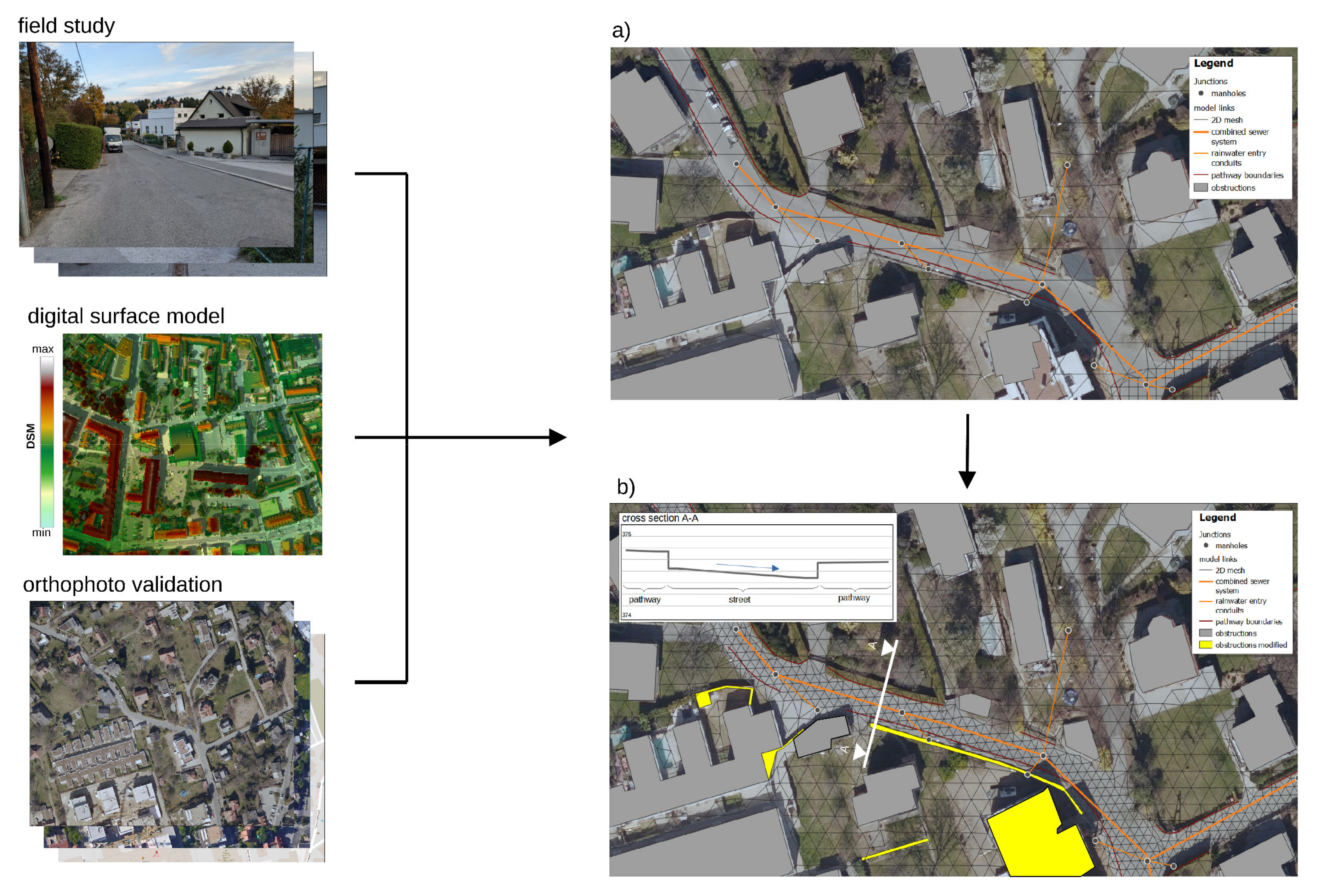
Two DEM based on airborne laser scan data (ALS) are available for the study site. The first DEMraw has a spatial resolution of 1 × 1 m. The second DEMmod include the modification of the micro-structures combined with a higher spatial resolution of 0.4 × 0.4 m. Wang et al. [43] demonstrated the importance of revising the DEM with urban micro-structures identified by a digital surface model (DSM). Additionally, culverts under bridges, micro-boundaries due to the flood paths along the streets and small walls along the private grounds must be considered. All these micro-structures influence water flow on the surface [43]. To quantify the impact of accurate terrain and obstruction data for urban flood analysis, these obstructions were revised based on Google Earth data, open data orthophotos (e.g., from https://basemap.at/ (accessed on 2 December 2021)), expert interviews and personal location inspections. Furthermore, the revised obstructions are integrated in the DEMmod. Based on these two DEMs, the spatial discretization of the surface runoff was generated with two different 2D meshes.
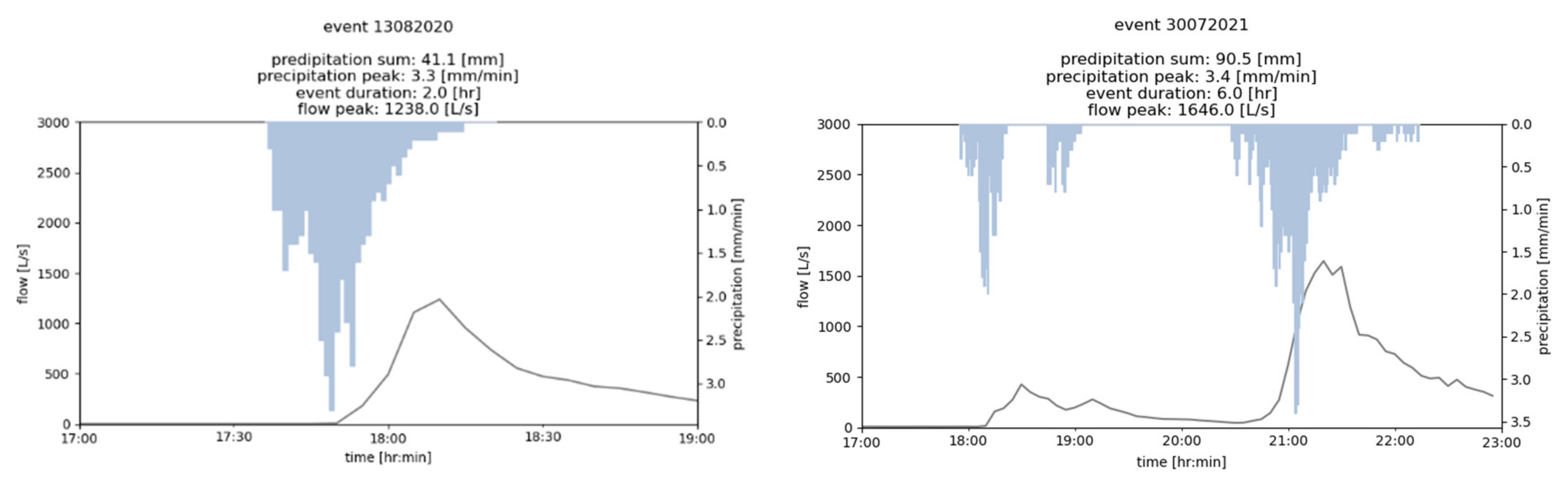
Two extreme storm events were observed in the catchment, one on 13 August 2020 with a return period of 90 years and one on 30 July 2021 with a return period greater than 100 years. Both events were convective storm events with high rainfall intensity and short event duration (Figure 3). The extreme storm event on 13 August 2020 was used to calibrate the model. The event on 30 July 2021 was used for the identification of the highest-impact uncertainty source. The precipitation data are measured by weighing precipitation gauge in the catchment (Figure 4) with a temporal resolution of one minute and measurement accuracy of 0.1 mm.
The required hydraulic and hydrological model parameters (e.g., surface roughness, hydrological losses, infiltration parameters) depend, among other factors, on the land cover. These data are provided by the surveying department of the city of Graz and were classified into six land cover classes (impervious, green areas, forest and trees, farmland, water areas and buildings (Figure 2)). The land cover types were revised with open data orthophotos (Google Earth, OpenStreetMap, basemap). The combined sewer network data (e.g., conduits, manholes, junctions, and special structures such as combined sewer overflows (CSO)) were provided by the operator, Holding Graz Water Management.
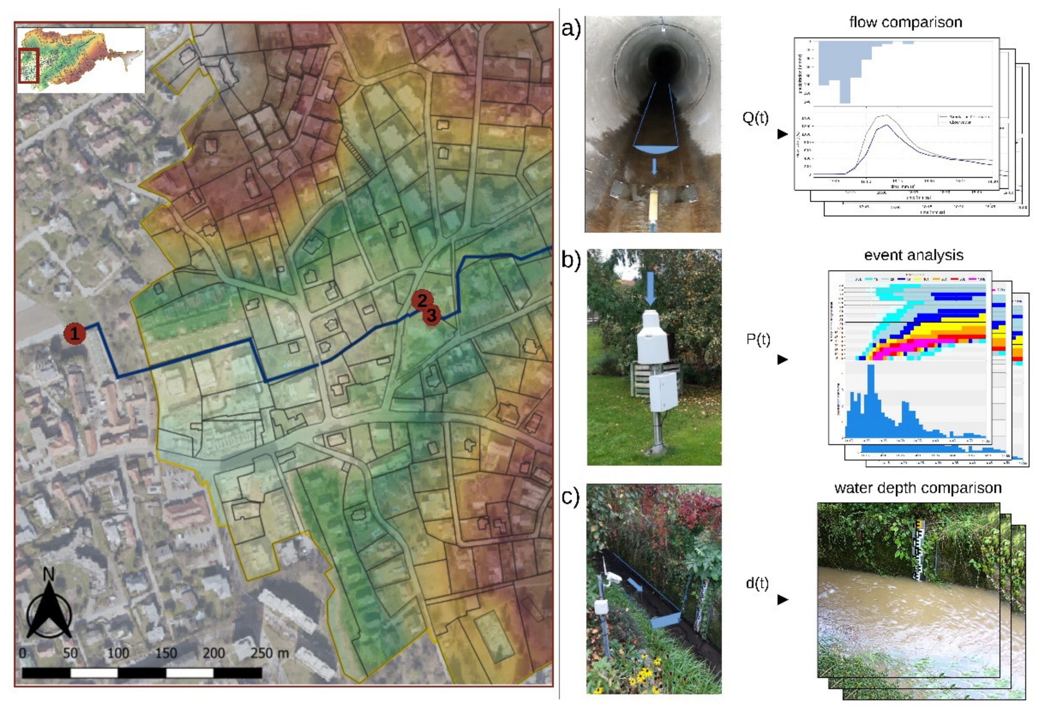
The available observation data are classified into quantitative and qualitative calibration data. The quantitative data stem from a portable flow measurement system (PCM-Pro) and a camera system that generates continuous photo series and videos of water depth gauges upon activation when a threshold water depth of 0.1 m is surpassed (Figure 4). Additionally, qualitative data, i.e., reported flood locations, based on emergency reports from local fire departments, were available. These include the locations and the severity of an emergency in the catchment. Further, spatial data on manhole clogging and sewer surcharging has been provided for the 13 August 2020 event. Both qualitative data and quantitative camera data are only available for the 30 July 2021 event. Therefore, the flow data and the damage data were selected to calibrate and validate the model. Both data sources were used to analyze the impact of the different uncertainty sources.
2.3. Uncertainty Source: Input Data
The flow direction of the modelled surface runoff is highly influenced by terrain data and its spatial resolution [56]. Therefore, the DEM represents one of the most sensitive model inputs. When structures such as buildings, walls, fences, and underpasses were not included, the calculated flow path resulted in unrealistic directions. One way to reduce this error was the revision of the DEM as the main input data to create the 2D mesh. A combination of information from web-based orthophotos (e.g., basemap, Google Maps, Google Earth or OpenStreetMap), the digital surface model (DSM) and field studies were used to identify microstructures impacting flow directions on the surface. Three main micro-structures were selected to work into the DEM and subsequently the 2D mesh (Figure 5):
- All micro-obstructions of the private and the public ground that obstruct flows (e.g., walls and fences);
- Validation of buildings with changes in geometry and implement new buildings that are not included in the old data source (e.g., land cover data);
- Take all pathway boundaries along the streets into account, including the gaps due to street entrances.
2.4. Uncertainty Source: Model Parameters
The sensitive model parameters on steep areas were optimized using the Sensitivity-based Radio Tuning algorithm (SRTC) which is demonstrated by [79]. The SRTC-algorithm can be described as a partial linear optimization algorithm that benefits from a suitable number of simulations due to the partwise linear approach. Non-linearity is approximated by the number of points within the selected parameter limits and an iterative validation simulation after the optimization.
Based on the study demonstrated by Liu et al. [48], the surface roughness, hydraulic conductivity and hydrological losses (i.e., interception and depression storage) have been identified as the parameters to calibrate in this research. Only locations with a high surface slope (>5 percent) were selected for calibration due to the hillside character (more than 70 percent of all hydraulic elements).
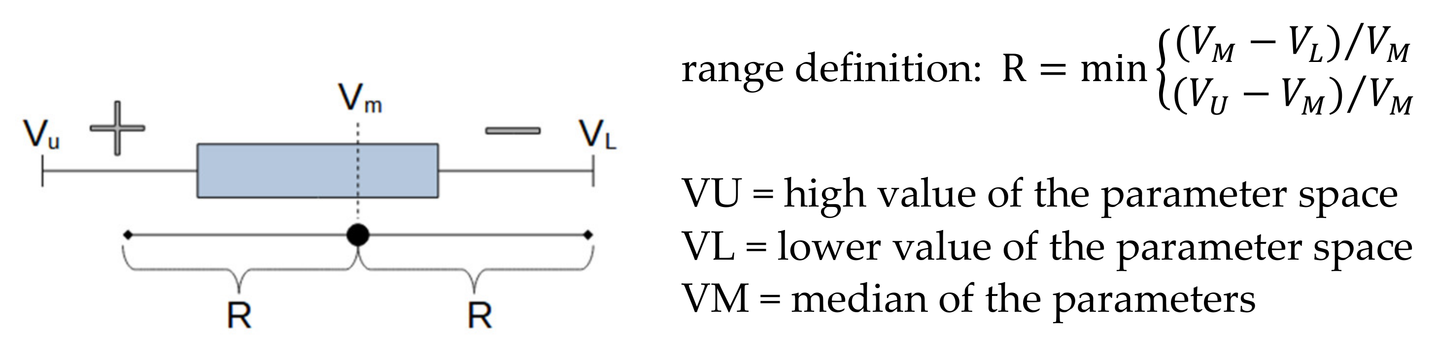
The SRTC algorithm started with an initial value as a reference scenario and varied within a predefined range (R) of realistic parameter values based on a comprehensive literature review (Appendix A.1.). For the definition of the parameter range, outliers in the parameter’s distribution were removed and the median was selected as the initial value. The outliers were defined as values over and under 1.5 times the interquartile range. For the variation of the parameters, the minimum of the difference to the upper or lower limit values was used to guarantee that the realistic parameter space is not exceeded (Figure 6).
Inside this range, eight sensitivity points were defined and each of them resulted in an independent simulation, leading to a total of 49 simulations. Due to the eight sensitivity points for each selected parameter, the non-linearity of the model could be considered. Based on the simulations, each sensitive model parameter could be varied individually and compared with the change of the observed time series (e.g., flow, water depth) by selected performance indicators. The variation of the parameter in hillside catchments depends on the surface slope. For example, the surface roughness as one key parameter was assumed to be higher on hillside areas than on flat terrain [57,58]. Equally, it can be assumed that the surface storage is lower in strongly sloped surfaces. This effect is described by the following relation between the surface slope, the depression storage in flat areas, and the spatial resolution of each land cover class. The complete description of Equation (1) is attached in Appendix A.2.
A = area of the 2D cell [m2]; DS = depression storage flat area [mm], = surface slope [–]; ds = reduced depression storage [mm].
The flow measurement data at the end of the catchment are used to compare the simulation results with the observation of the heavy storm event on 13 August 2020. Three objective functions are used to quantify the performance of the urban flood model (Nash-Sutcliff-Efficiency (NSE), Peak Error (PE), Volumen Error (VE)). VE and NSE were selected to evaluate the complete event on the one hand and the important peak flow value PE on the other hand.
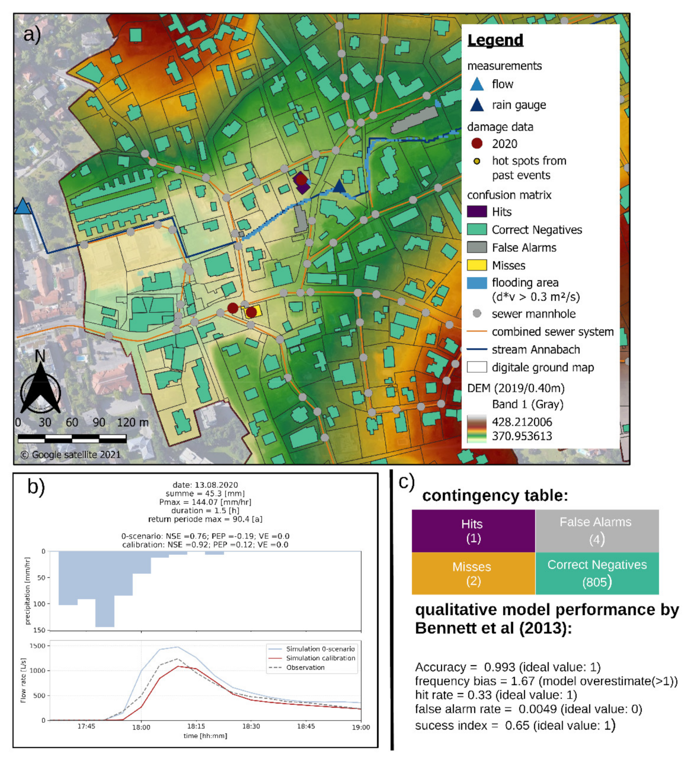
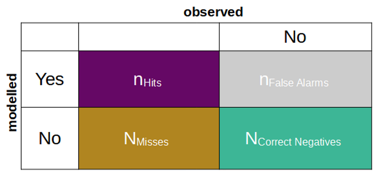
The second step was the validation of the urban flood model with the optimum parameter set after the calibration. The defined flooding areas were compared with the operating transcripts of the fire department, public interviews of affected persons, photo and video documentation of the sewer operator for the 13 August 2020 heavy storm event in a qualitative way. This is recommended to assess not only the temporal variation of the flow at one specific measurement point, but also the spatial distribution of the flooding area in the whole catchment area. Therefore, it is essential to determine the threshold value for the definition of the inundation area as well as the appropriate model variable. Previous studies based on experimental tests have demonstrated that a combination of flow velocity and water depth should be used to define the flooding area [80,81] with a threshold value of 0.3 m2/s [82]. Based on these values, the simulated flooding area can be compared with the observations of damages and quantified by the creation of the contingency table [83]. The following qualitative performance indicators based on the confusion matrix are selected to quantify the model quality and are attached to Appendix A.3. (model accuracy, frequency bias, hit rate, false alarm rate and success index).
2.5. Uncertainty Source: Model Structure
2.5.1. D/2D Urban Flood Model
The commercial modeling software PCSWMM2D (version 7.4.3240) [84] by CHI-Water (https://www.pcswmm.com/ (accessed on 22 December 2021)) was used for this study. The implemented urban flood model is based on the EPA Storm Water Management Model (SWMM) 5.1 [28]. This model was frequently applied in the field of urban drainage modeling (e.g., [85,86,87]). The model combines two general model types. A cell-based approach for spatial discretization resulting in a raster with a predefined spatial resolution and geometry (2D cells). This approach was similar to models based on cellular automata (CA) such as LISFLOOD-FP [88]. The full hydrodynamic 1D de Saint-Venant equations (continuity equation (Equation (2)) and conservation of momentum (Equation (3)) solved the water transport between each 2D cell. This resulted in a 2D mesh consisting of nodes and open conduits to determine water depth in each node and flow velocity in each conduit. Therefore, both models 1D and 2D can be described by the same mathematical formulations (Equation (2) and Equation (3)), which allows the use of the same timestep in both models. Each 2D cell represented one specified land cover class, allowing the determination of each relevant hydrological subprocess (infiltration, precipitation, evapotranspiration, or snow melting) for the generation of the surface runoff in a fully distributed way.
The implicit backwards Euler method is used to solve the 1D de Saint-Venant equations [89]. The appropriate choice of the variable time step depends primarily on the spatial discretization of the 2D surface. For this reason, the resolution of the 2D mesh is the key parameter regarding the required computational effort.
x = distance [m]; t = time [sec]; A = cross area [m²]; Q = flow rate [m³/sec]; H = hydraulic head [m]; Sf = friction slope [–]; hL = local energy loss [-]; g = acceleration of gravity [m/sec²].
Water transport in the sewer system is also determined by the full 1D de Saint-Venant equations. To determine the head at the nodes, the difference between inflow and outflow in the linked conduits is equal to the time difference of the volume for normal flow conditions (Equation (4)). If at one time-step all connected conduits are pressurized, the nodal continuity equation (Equation (5)) must be replaced with a perturbation equation (Equation (5)) [89].
V = node assembly volume [m³]; t = time [sec]; ASN = node assembly surface area [m²]; ASL = surface area of connected links; Q = flow rate [m³/sec]; H = hydraulic head [m]; DH = adjustment to the node head [m]; Cd = discharge coefficient [-]; A0 = open area [m²]; [-]; g = acceleration of gravity [m/sec²]; He = head difference [m].
The bidirectional connection between the surface and the sewer system is described with a bottom orifice as a hydraulic element in the model. The interaction with the surface in the case of a sewer surcharging is given by the Torricelli’s law in Equation (6) and needs only the water depth in the sewer node or the water depth on the connected surface node of the 2D Mesh. A detailed description of the mathematical formulation of the flow routing in the conduits and the exchange between the sewer system and the surface is given by Rossman [89].
Rainfall volume coming from buildings is considered in two ways in the model. The rainfall on the buildings erected before 2005 is directly connected to the sewer system. All other buildings drain the rainwater directly on the surface. This assumption had to be made due to a new regulation implemented by the city of Graz since 2005, specifying that stormwater cannot discharge directly into the sewer system.
2.5.2. D Model
The 2D model used the same approach to calculate the flooding areas as the 1D/2D model scenario. This resulted in the combination of the CA-approach and solving of the full 1D de Saint-Venant equations for the water transport between the cells. The surface runoff as the input for each cell based on the land cover class. The only difference to the 1D/2D model scenario is to ignore all processes of the sewer system such as sewer surcharging or sewer overflows. This resulted in a 2D model that only considered the surface runoff and the discharge in the stream.
2.6. Identification of Uncertainty Source
The main study objective is to identify the most impact of the three analyzed uncertainty sources: (i) influence of the DEM quality and resolution as one main input data for urban flood models; (ii) influence of three selected sensitive model parameters (surface roughness, hydrological losses, hydraulic conductivity); (iii) impact of the sewer system as one main element of the model structure. However, the presented method is designed for general usability, allowing it to analyze the impact of any source of uncertainty.
Model uncertainty is defined as the difference between the simulated and the observed objective value under consideration of all possible errors [51]. Therefore, the empirical variance as the mean squared deviation from the empirical mean value is suitable to quantify the impact of different uncertainty sources on the model, depending on the selected model variable. This is described with the uncertainty value UCk (Equation (12)). In this study, two measurement sites with different physical values (water depth and flow) are available. This allows the analysis of uncertainty sources with the highest impact on these two variables.
= simulated value at a timestep t; = observed value at a timestep t; = relative diviation at a timestep t; = vector of the relative deviation for each scenario s; Rs = range of each scenario s; = difference of range between two scenarios i and j; = mean value of all comparisons; UCk = uncertainty value of each comparison k; = empirical variance of the compared scenarios ; = identifier of the most impact uncertainty source.
First, the range (Rs) of the relative deviation for each of the eight scenarios and both model variables is determined using the differences between the observation and the simulation at each reported timestep (). Each of the three uncertainty sources has two options:
- DEMraw and DEMmod (input data);
- Sensitive model parameters with literature values and calibrated values (parameters);
- 1D/2D model and 2D model (model structure).
Consequently, four relative scenario comparisons regarding each source are used to estimate the value. The maximum of each UC value represented the identifier for the most impact uncertainty source UCmax (Equation (13)).
3. Results & Discussion
3.1. Model Calibration and Validation
The first step in the model evaluation was to optimize the sensitive model parameters at the point where the flow measurement system in the Annabach stream is situated (Figure 4). This step can be described as the quantitative model evaluation part.
Three sensitive hydrological parameters (hydrological losses, hydraulic conductivity and surface roughness) and one hydraulic model parameter (surface roughness) are used to calibrate the model. The surface roughness value in the hydrological model is also used for the hydraulic surface model. Each parameter was classified into six land-cover classes, which are generally divided into impervious and pervious areas.
Eight sensitivity points are used by the SRTC algorithm, and this resulted in 48 simulations to find the optimal parameter setup. Each scenario with the base DEM needs 1.5 h (minimum timestep of 0.15 sec) and for the revised DEM with the detailed 2D mesh 12 h (minimum timestep of 0.10 sec) to simulate the event of 13 August 2020 with a total event time of five hours. An Intel (R) Core (TM) i7-7700 CPU with 3,60 GHz and 16 GB RAM was used for all simulations. After the optimization and the validation with the SRTC algorithm, an optimized parameter vector can be determined (calibration value in Table 1).
The calibrated model resulted in good model performance in the corresponding reference point after the optimization, which is quantified by an NSE from 0.76 to 0.92, the PE from −0.18 to 0.12 and the low VE from zero. The influence of steep surface on the accurate model parameter selection can be assessed, because only the sensitive parameters in the hillside area are optimized. The results of the parameter optimization demonstrate that especially the roughness parameter should be increased in hillside areas. This also confirms the hypothesis to separate the parameter set-up in hillside areas from those in flat areas, which was derived from the studies demonstrated by LUBW [57] and USDA [58].
Moreover, the surface flow is based on the 1D de Saint-Venant equations in the ordinary global coordinate system. Juez et al. [90] recommend a transformation of the gravitation terms in the equations in a local coordinate system if a steep slope condition occurs. This is especially relevant if sediment transport processes and granular flows are investigated. The differences between the use of a global coordinate system and a local coordinate system can be compensated by increasing the roughness parameter in a realistic range [91]. Additionally, the effects are relevant for events with long durations. This could also be confirmed by the results of the calibration. Therefore, the calibration represents an essential part, especially if the traditional mathematical formulations and solving of the 1D de Saint-Venant equations are used. In contrast, the results of the calibration do not indicate a reduction of hydrological losses in hillside areas. Although this should occur due to the geometric relationships (Equation (1)). One possible explanation is that the precondition of the water content in the soil zones and the surface storage is considered as a very simplified initial condition in the model, which resulted in an undersized starting storage capacity [92]. Therefore, it can be deduced that even in event-based modeling, the pre-condition on the soil zones must always be analyzed in detail.
The qualitative evaluation represents the second part of the model evaluation. The results of the calibrated model are the basis for the qualitative evaluation, which aimed to verify the spatial distribution of the flooding areas in the whole catchment. This resulted in a model accuracy of 0.993 (best value 1), success index of 0.65 (best value 1) and a frequency bias of 1.67, which is an indicator that the model overestimates the flooding areas (frequency bias >1).
Based on the presented quantitative model calibration and qualitative model validation the spatial and temporal distribution of the flooding event on 13 August 2020 could be evaluated in a sufficient way (Figure 7). For this reason, the presented combination of two evaluation methods is suitable to evaluate the spatial and temporal distribution of the flooding processes, which results in a more robust model.
In addition, the simulation with the second event on 30 July 2021 confirms the selection of the sensitive calibrated model parameters in hillside areas, especially the surface roughness (NSE = 0.91, PE = 0.07, VE = 0.2).
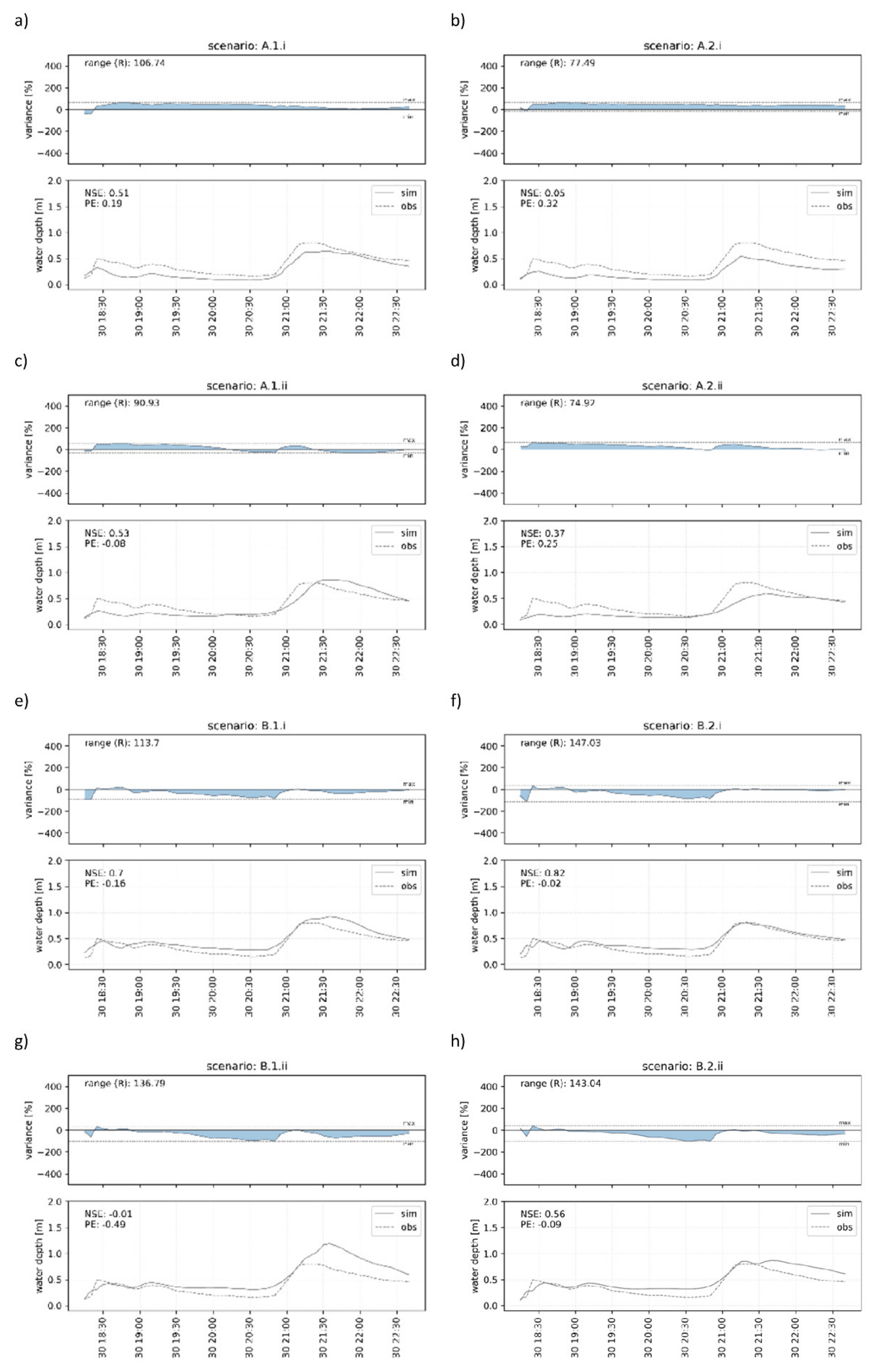
3.2. High-Impact Uncertainty Sources
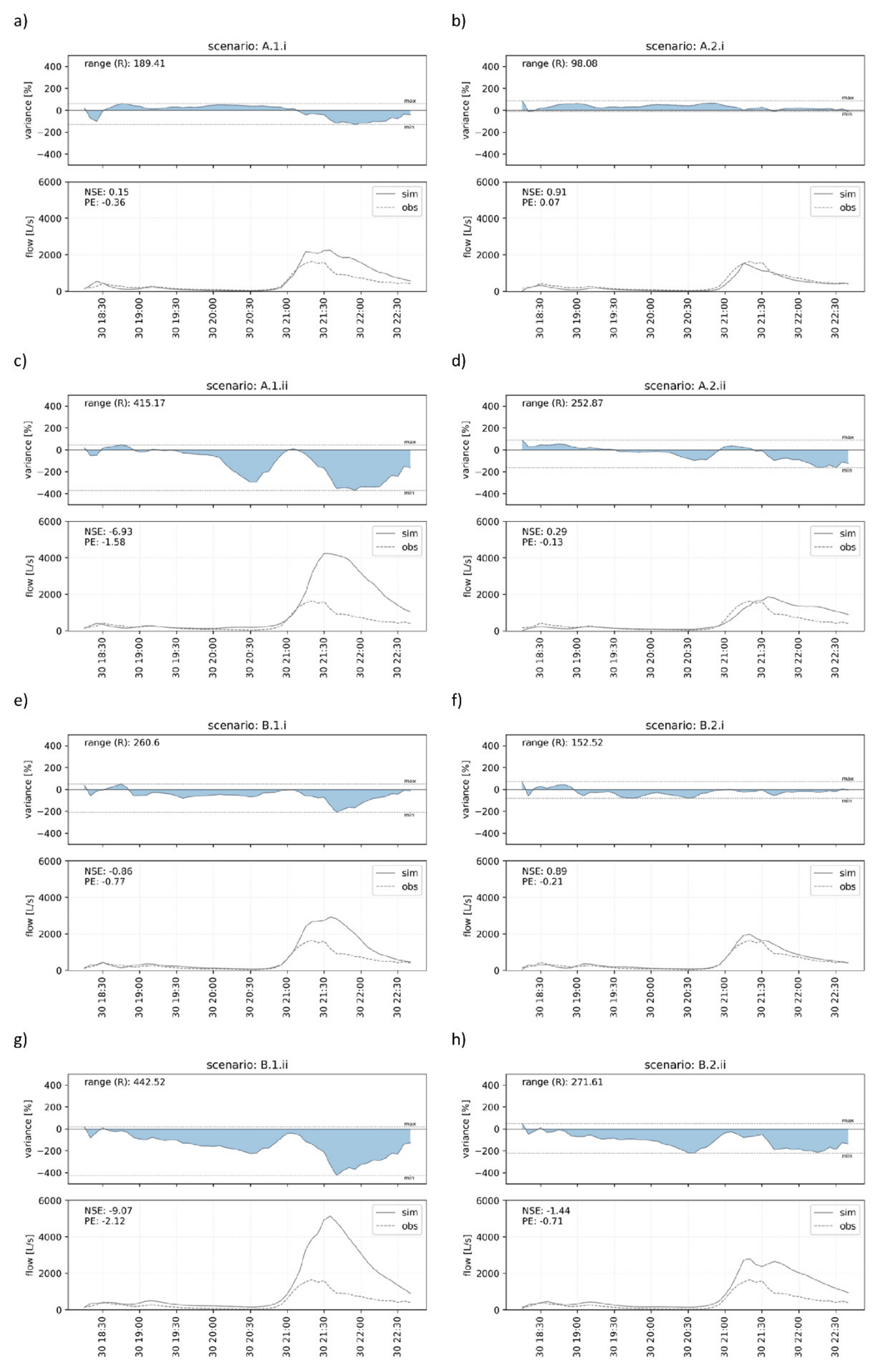
For the identification of the uncertainty sources with the highest impact, the event on 30 July 2021 is analyzed at two monitoring sites and consequently two variables, flow (Figure 8) and water depth (Figure 9). The range of the relative deviation (Rs) represents the value to quantify the impact of uncertainties. The presented NSE and PE are model performance indicators in comparison to the measurements for each of the analyzed scenarios. Rs is used to determine the UCk value for each scenario. This is required to identify the highest source of uncertainty and is not an indicator of model performance. This value can also be used to support the communication of uncertainties as, for example, required by Grayson and Blöschl [50] and Teng et al. [27].
The best model performance for the variable flow represents scenario A.2.i (Figure 8b) quantifies with the NSE of 0.91, which is in a similar range as scenario B.2.i with the NSE of 0.89 (Figure 8f). This is an indicator that the calibration of the model and the model structure have a high influence on the model performance. The best model performance of scenario B.2.i with an NSE of 0.82 regarding the variable water depth confirms these conclusions (Figure 9f).
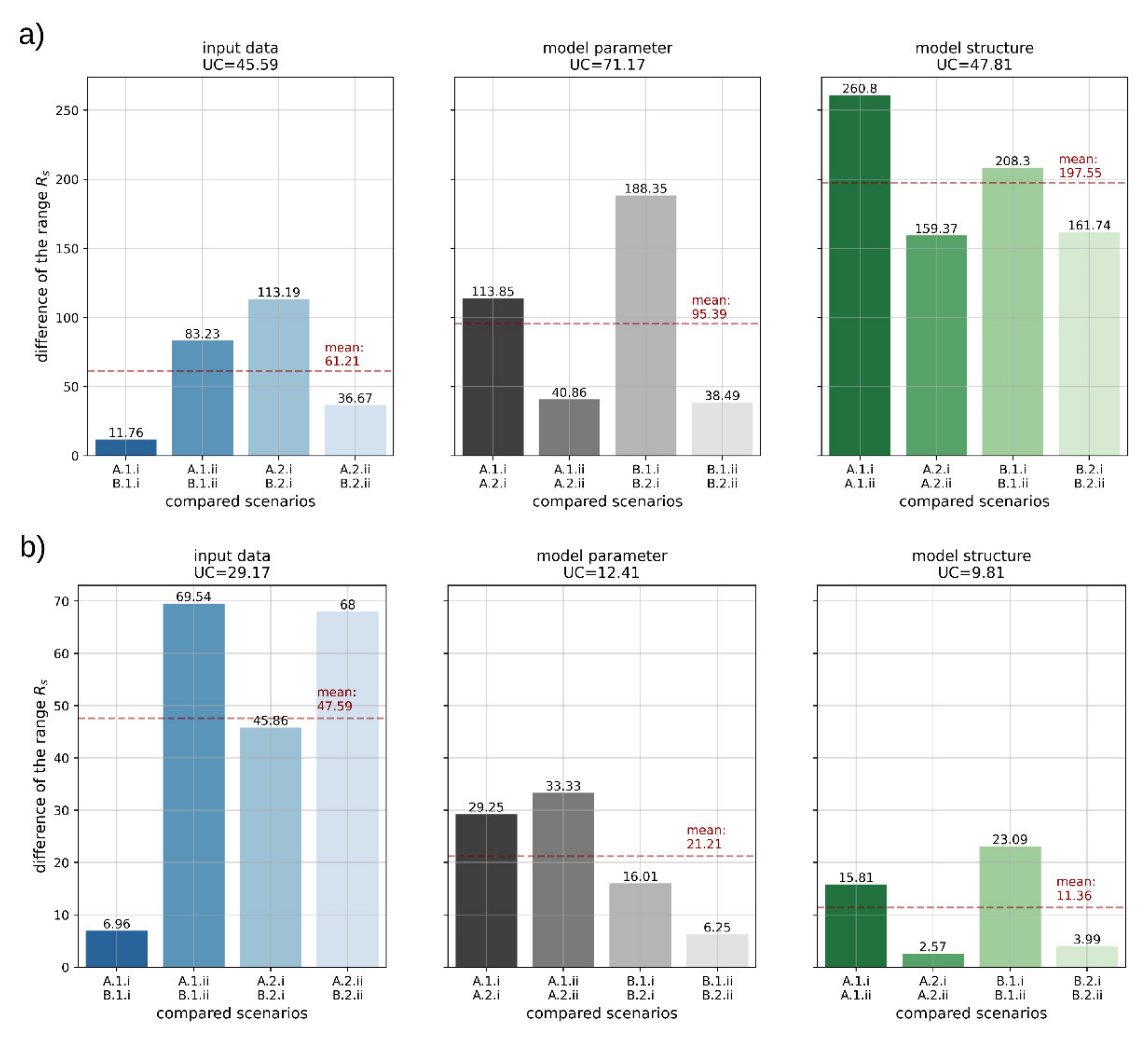
The comparison between the results of the eight scenarios regarding the variables flow and water depth shows a significant difference in the relative deviation range (Rs). The difference between the maximum and the minimum Rs of all eight simulated scenarios for variable flow is 344.49. In contrast, the difference for water depth is only 72.11. The identification of the highest-impact uncertainty source is dependent on the selected variable and the corresponding monitoring sites. For this reason, the interpretation of results regarding the high-impact uncertainty source is differentiated by the two variables flow (Figure 10a) and water depth (Figure 10b).
The resulting UC values for the uncertainty source input data regarding both variables are in a similar range (45.59 for flow and 29.17 for water depth). The same UC for the uncertainty source model parameter is about 71.17 for flow. In contrast, the UC value of water depth is 12.41. The UC values for the model structure as the uncertainty source are 47.81 for flow and 9.81 for water depth.
In comparison to the model parameter and model structure, the UC value regarding the flow and the input data as uncertainty source has the lowest value, but this UC has the highest value for the assessment in terms of the water depth. Thus, it can be derived that an improvement of the input data (validation of the micro-structures and higher resolution of the DEM) is only useful in the case of an assessment of the urban flooding concerning the water depth.
If the flow on the surface must be considered for an urban flood assessment, the optimization of the sensitive model parameters has the highest impact in hillside catchments (UC = 71.17). In particular, the optimization of the surface roughness in steep locations is impactful. This conclusion must be re-evaluated if a model is used with the formulation of the mathematical equations in a local coordinate system because this represents the flow characteristics more realistic at a steep surface [90,91]. In contrast, an optimization of the model parameters for an evaluation concerning the water depth does not have a large impact (UC = 12.41). Similar conclusions are reached by Hunter et al. [56], who identify model calibration as a useful way to reduce uncertainties in urban flooding modeling.
The influence of the sewer system as a source of uncertainty in the model structure has the most impact in terms of the absolute deviations of all four compared scenarios concerning the flow with of 197.55 (Figure 10a). This also confirms the conclusions of Dong et al. [38], GebreEgziabher and Demissie [39], and Zhou et al. [40]—that the sewer system can not be discarded in terms of urban flooding. Furthermore, a simplified approach with source and sink terms, as demonstrated by Wang et al. [43], should be used carefully.
In summary, the sensitive model parameters are identified as the highest-impact uncertainty source regarding the variable flow for urban flood modeling in hillside catchments. Therefore, especially when assessing the urban flood risk using damage functions that consider water depths and flow, the selection of sensitive model parameters (e.g., surface roughness) in the course of calibration is essential. If the water depth is the selected variable, the improvement of the DEM as the input data has the highest impact compared to the uncertainty sources model parameter and model structure. Therefore, the validation of microstructures and the resolution of the DEM represent the main potential to reduce the uncertainty in this context. In addition, the combination of a DEM revision, the optimization of sensitive model parameters and the use of a 1D/2D model as a general model structure provide the best results. Similar conclusions are expected in catchments with flat terrain conditions but need further investigation.
4. Conclusions
The focus of the study was to identify the most impact of three main uncertainty sources (input data, model parameter, model structure) in terms of urban flood modeling in a hillside study site. To identify the high impact source, a transferable variance-based approach with only one value (UC) was developed by using two monitoring sites and two variables (flow and water depth).
In general, the variable water depth represents the lower sensitive variable, which is demonstrated by the range of relative deviation (Ri) between simulations and observations (maximum Ri of 442.52 percent (flow) and maximum Ri of 147.03 percent (water depth)). Therefore, the main conclusions differentiated between the two available variables. The calibration of the sensitive model parameter represents the most-impact uncertainty source regarding the variable flow (UC = 71.17). Additionally, the high mean value of 197.55 ( for the uncertainty source model structure indicates the importance of the sewer system in terms of urban flooding in hillside catchments. For this reason, an urban flood model should include the sewer system. The comparisons of the eight scenarios with the observations confirm this conclusion because the scenarios with the 1D/2D model as model structure provide the best results (NSE of 0.91 for flow and NSE of 0.82 for water depth). The input data represents the high-impact uncertainty source if the water depth is selected as the relevant variable (UC = 29.17). Especially the validation of micro-structures (walls, pathway boundaries, buildings) resulted in good adaptions regarding the water depth (NSE of 0.82). Other input data such as spatially distributed precipitation can represent a further relevant uncertainty source, but they are not analyzed in this study.
The presented study includes only one hillside catchment and two real heavy storm events. For robustness of the derived conclusions, it is desirable to test the same method in several catchments with hillside locations and further real heavy storm events. Furthermore, it should be clear that not every possible uncertainty source can be analyzed in one study, but the results provide an initial picture regarding uncertainties in terms of urban flood modeling in hillside catchments.
Author Contributions
Conceptualization, S.R., G.K. and D.M.; methodology, S.R.; software, S.R.; validation, S.R.; formal analysis, S.R.; investigation, S.R.; data curation, S.R.; writing—original draft preparation, S.R.; writing—review and editing, S.R., G.K., M.P. and D.M.; visualization, S.R., M.P.; supervision, D.M.; project administration, D.M.; funding acquisition, D.M. All authors have read and agreed to the published version of the manuscript.
Funding
This research was funded by the Provincial Government of Styria in terms of the Interreg Central Europe Project RAINMAN (Interreg Central Europe Project CE968: https://www.interreg-central.eu/Content.Node/RAINMAN.html (accessed on 08 February 2022)). Additionally, the research was supported by Open Access Funding by the Graz University of Technology.
Data Availability Statement
All used data are provided by the city of Graz to build-up the model and for the model calibration the Institut of Urban Water Management and Landscape Engineering. These can be provided on request.
Acknowledgments
We want to thank all partners of the RAINMAN project team for their great work, input, and funding of this research. We would also like to thank numerous departments of the city Graz, who supported this work with the data to build-up the urban flood model. Additionally a big thank you to Computational Hydraulics International (CHI-Water) which supports this research by using the software PCSWMM2D. A special thank you goes to Michael Pointl and Albert Wilhelm König who supported this work through numerous discussions regarding paper structure and language style. A primary thank you to both reviewers which support this research with helpful comments.
Conflicts of Interest
The authors declare that they have no known competing financial interests or personal relationships that could have appeared to influence the work reported in this paper. The funders had no role in the design of the study; in the collection, analyses, or interpretation of data; in the writing of the manuscript, or in the decision to publish the results.
Appendix A
Appendix A.1. Overview of Sensitive Model Parameters of the Flooding Process

Table A1.
Overview of the model parameters surface roughness for urban flood models.
| Model Parameter: Surface Roughness [m-1/3/1] | ||||||
|---|---|---|---|---|---|---|
| Source | Impervious | Green Area | Trees and Bushes | Farmland | Water | Buildings |
| [93] | 0.12 | 0.352 | 0.3 | 0.09 | - | 0.011 |
| [45] * | 0.014 | - | 0.189 | 0.043 | 0.022 | 0.074 |
| [94] * | 0.048 | 0.275 | 0.4 | - | - | - |
| [95] | 0.015 | 0.28 | 0.45 | 0.02 | - | - |
| [51] | 0.015 | 0.28 | 0.45 | 0.02 | - | - |
| [48] * | 0.0176 | 0.285 | - | - | - | 0.012 |
| [57] | 0.036 | 0.233 | 0.25 | 0.096 | 0.0953 | 0.018 |
| [96] | 0.0155 | 0.3250 | 0.6 | 0.115 | - | - |
| [97] | 0.0105 | 0.014 | 0.012 | - | - | 0.0125 |
| [98] | 0.0125 | 0.2 | 0.25 | 0.04 | 0.02 | 0.05 |
| [99] | 0.0155 | 0.253 | - | 0.12 | 0.12 | 0.15 |
| [100] | 0.0105 | 0.065 | 0.12 | 0.038 | - | 0.035 |
* calibrated values.
Table A2.
Overview of the model parameters surface roughness for urban flood models.
| Model Parameter: Losses [mm] | |||||
|---|---|---|---|---|---|
| Source | Impervious | Green Area | Trees and Bushes | Farmland | Buildings |
| [101] | 1.88 | 3.75 | 8 | - | - |
| [102] * | 2.34 | 9.64 | 13.26 | 12.55 | - |
| [103] ** | 3 | 9 | 11.67 | 9 | 4 |
| [59] | 0.9 | 4 | 4 | 8.28 | 0.9 |
| [104] *** | 1.2 | 5.55 | 7.46 | 5.83 | 0.74 |
| [48] *** | 2 | 6 | 10 | - | 2 |
| [105] | 0.8 | 4.8 | 6.2 | 3.25 | - |
| [61] | 2.07 | 7.65 | 8.28 | 8.28 | 4.23 |
* interception and depression storage; ** only depression storage; *** calibrated values.
Table A3.
Overview of the parameter hydraulic conductivity for urban flood models.
| Model Parameter: Hydraulic Conductivity [mm/h] | |||||||||
|---|---|---|---|---|---|---|---|---|---|
| Source | Sand | Loamy Sand | Sandy Loam | Loam | Siltloam | Sandy Clayloam | SandyClay | Silty Clay | Clay |
| [106] | 11.4 | 7.6 | 7.6 | 3.8 | 1.3 | 1.3 | 1.3 | 1.3 | 1.3 |
| [107] * | 360 | 11.7 | - | 2.34 | - | - | - | - | 0.44 |
| [108] | 210 | - | - | 13.2 | - | - | - | - | 0.6 |
| [109] | 297 | - | - | 2.6 | - | 13.1 | - | - | 2.6 |
| [110] | 150 | - | 3.5 | - | - | 4.5 | - | 0.54 | - |
| [111] | 120.34 | 29.97 | 10.92 | 3.3 | 6.6 | 1.52 | 1.02 | 0.51 | 0.25 |
| [99] | 210 | 61 | 26 | 13 | 6.8 | 4.3 | 1.2 | 0.9 | 0.6 |
| [112] | - | - | 44.2 | 10.4 | 4.5 | 13.08 | - | - | 2.58 |
* experimental values.
Appendix A.2. Reduction of the Depression Storage in Hillside Areas
Figure A1.
Conceptual approach to reduce the model parameter depression storage depending on the surface slope.
Figure A1.
Conceptual approach to reduce the model parameter depression storage depending on the surface slope.

Appendix A.3. Qualitative Objective Functions
Figure A2.
Definition of the contingency table values (Hits, False Alarms, Misses, Correct Negatives) as qualitative comparison between modelled and observed flooded areas [113].
Figure A2.
Definition of the contingency table values (Hits, False Alarms, Misses, Correct Negatives) as qualitative comparison between modelled and observed flooded areas [113].

Appendix A.4. Quantitative Objective Functions
References
- Kundzewicz, Z.W.; Ulbrich, U.; Brücher, T.; Graczyk, D.; Krüger, A.; Leckebusch, G.C.; Menzel, L.; Pińskwar, I.; Radziejewski, M.; Szwed, M. Summer Floods in Central Europe–Climate Change Track? Nat. Hazards 2005, 36, 165–189. [Google Scholar] [CrossRef]
- The Mediterranean Region under Climate Change: A Scientific Update; Moatti, J.-P.; Thiébault, S. (Eds.) IRD Éditions: Marseille, France, 2016; ISBN 978-2-7099-2219-7. [Google Scholar]
- Berndtsson, R.; Becker, P.; Persson, A.; Aspegren, H.; Haghighatafshar, S.; Jönsson, K.; Larsson, R.; Mobini, S.; Mottaghi, M.; Nilsson, J.; et al. Drivers of changing urban flood risk: A framework for action. J. Environ. Manag. 2019, 240, 47–56. [Google Scholar] [CrossRef] [PubMed]
- O’Donnell, E.C.; Thorne, C.R. Drivers of future urban flood risk. Philos. Trans. R. Soc. London. Ser. A Math. Phys. Eng. Sci. 2020, 378, 20190216. [Google Scholar] [CrossRef] [PubMed] [Green Version]
- IPCC. Global Warming of 1.5 °C. An IPCC Special Report on the Impacts of Global Warming of 1.5 °C above Pre-Industrial Levels and Related Global Greenhouse Gas Emission Pathways, in the Context of Strengthening the Global Response to the Threat of Climate Change, Sustainable Development, and Efforts to Eradicate Povertyte; lntergovernmental Panel on Clima Change: Geneva, Switzerland, 2018. [Google Scholar]
- Ashley, R.M.; Balmforth, D.J.; Saul, A.J.; Blanskby, J.D. Flooding in the Future–Predicting Climate Change, Risks and Responses in Urban Areas. Water Sci. Technol. 2005, 52, 265–273. [Google Scholar] [CrossRef] [PubMed]
- Freddy, V.; El Mehdi Saidi, M.; Douvinet, D.; Fehri, N.; Nasrallah, W.; Menad, W.; Mellas, S. Urbanization and Land Use as a Driver of Flood Risk. In The Mediterranen Region under Climate Change; Institut de Recherche Pour Le Développement Marseille; Ird Éditions Institut De Recherche Pour Le Développement: Marseille, France, 2016; pp. 563–575. ISBN 978-2-7099-2219-7. [Google Scholar]
- Trenberth, K.E. Changes in precipitation with climate change. Clim. Res. 2011, 47, 123–138. [Google Scholar] [CrossRef] [Green Version]
- Kundzewicz, Z.W.; Pińskwar, I.; Brakenridge, G. Changes in river flood hazard in Europe: A review. Hydrol. Res. 2018, 49, 294–302. [Google Scholar] [CrossRef]
- Davis, R. Flood and Hight Water Marks. Available online: http://floodlist.com/dealing-with-floods/flood-high-water-marks (accessed on 25 December 2021).
- Dankers, R.; Hiederer, D. Extreme Temperatures and Precipitation in Europe: Analysis of a High-Resolution Climate Change Scenario; The Publications Office of the European Union: Luxembourg, 2008. [Google Scholar]
- Nikulin, G.; Kjellstrom, E.; Hansson, U.; Strandberg, G.; Ullerstig, A. Evaluation and future projections of temperature, precipitation and wind extremes over Europe in an ensemble of regional climate simulations. Tellus A: Dyn. Meteorol. Oceanogr. 2011, 63, 41–55. [Google Scholar] [CrossRef] [Green Version]
- ZAMG Vermehrte Starkniederschläge? Available online: https://www.zamg.ac.at/cms/de/klima/informationsportal-klimawandel/klimavergangenheit/neoklima/starkniederschlag (accessed on 4 February 2021).
- Westra, S.J.; Fowler, H.J.; Evans, J.P.; Alexander, L.V.; Berg, P.R.; Johnson, F.; Kendon, E.J.; Lenderink, G.; Roberts, N.M. Future changes to the intensity and frequency of short-duration extreme rainfall: Future intensity of sub-daily rain-fall. Rev. Geophys. 2014, 52, 522–555. [Google Scholar] [CrossRef]
- KLIWA. Starkniederschläge Entwicklung in Vergangenheit Und Zukunft–Kurzbericht; Arbeitskreis KLIWA: Offenbach, Germany, 2019. [Google Scholar]
- Lehmann, J.; Coumou, D.; Frieler, K. Increased record-breaking precipitation events under global warming. Clim. Chang. 2015, 132, 501–515. [Google Scholar] [CrossRef]
- Berg, P.M.V.D.; Moseley, C.; Haerter, O.J. Strong increase in convective precipitation in response to higher temperatures. Nat. Geosci. 2013, 6, 181–185. [Google Scholar] [CrossRef]
- Pall, P.; Allen, M.R.; Stone, D.A. Testing the Clausius–Clapeyron constraint on changes in extreme precipitation under CO2 warming. Clim. Dyn. 2007, 28, 351–363. [Google Scholar] [CrossRef]
- Yin, J.; Ye, M.; Yin, Z.; Xu, S. A review of advances in urban flood risk analysis over China. Stoch. Hydrol. Hydraul. 2015, 29, 1063–1070. [Google Scholar] [CrossRef]
- Maier, R.; Krebs, G.; Pichler, M.; Muschalla, D.; Gruber, G. Spatial Rainfall Variability in Urban Environments—High-Density Precipitation Measurements on a City-Scale. Water 2020, 12, 1157. [Google Scholar] [CrossRef] [Green Version]
- Sapountzis, M.; Kastridis, A.; Kazamias, A.-P.; Karagiannidis, A.; Nikopoulos, P.; Lagouvardos, K. Utilization and Uncertainties of Satellite Precipitation Data in Flash Flood Hydrological Analysis in Ungauged Watersheds. Glob. NEST J. 2021, 23, 388–399. [Google Scholar] [CrossRef]
- Wild, T.; Dempsey, N.; Broadhead, A. Volunteered information on nature-based solutions–Dredging for data on deculverting. Urban For. Urban Green. 2019, 40, 254–263. [Google Scholar] [CrossRef]
- Plumb, B.D.; Juez, C.; Annable, W.K.; McKie, C.W.; Franca, M.J. The impact of hydrograph variability and frequency on sediment transport dynamics in a gravel-bed flume. Earth Surf. Process. Landforms 2019, 45, 816–830. [Google Scholar] [CrossRef]
- Galloway, G.; Brody, S.; Reilly, A.; Highfield, W. The Growing Threat of Urban Flooding; University of Maryland, Center for Disaster Resilience: College Park, MD, USA, 2018. [Google Scholar]
- Henonin, J.; Russo, B.; Mark, O.; Gourbesville, P. Real-time urban flood forecasting and modelling–A state of the art. J. Hydroinform. 2013, 15, 717–736. [Google Scholar] [CrossRef]
- Salvadore, E.; Bronders, J.; Batelaan, O. Hydrological modelling of urbanized catchments: A review and future directions. J. Hydrol. 2015, 529, 62–81. [Google Scholar] [CrossRef]
- Teng, J.; Jakeman, A.J.; Vaze, J.; Croke, B.F.W.; Dutta, D.; Kim, S. Flood inundation modelling: A review of methods, recent advances and uncertainty analysis. Environ. Model. Softw. 2017, 90, 201–216. [Google Scholar] [CrossRef]
- Rossman, L.A. Storm Water Management Model User’s Manual Version 5.1; US EPA National Risk Management Research Laboratory: Cincinnati, OH, USA, 2015. [Google Scholar]
- Vetsch, D.; Siviglia, A.; Bürgler, M.; Caponi, F.; Ehrbar, D.; Facchini, M.; Faeh, R.; Farshi, D.; Gerber, M.; Gerke, E.; et al. System Manuals of BASEMENT, Version 2.8.2; ETH Zurich, Laboratory of Hydraulics, Glaciology and Hydrology: Zurich, Switzerland, 2022; Available online: http://people.ee.ethz.ch/~basement/baseweb/download/documentation/BMdoc_System_Manual_v2-8-2.pdf (accessed on 23 May 2022).
- Ghimire, B.; Chen, A.S.; Guidolin, M.; Keedwell, E.C.; Djordjevic, S.; Savic, D. Formulation of a fast 2D urban pluvial flood model using a cellular automata approach. J. Hydroinform. 2013, 15, 676–686. [Google Scholar] [CrossRef] [Green Version]
- Guidolin, M.; Chen, A.; Ghimire, B.; Keedwell, E.C.; Djordjević, S.; Savić, D.A. A weighted cellular automata 2D inundation model for rapid flood analysis. Environ. Model. Softw. 2016, 84, 378–394. [Google Scholar] [CrossRef] [Green Version]
- Schmitt, T.G.; Thomas, M.; Ettrich, N. Analysis and modeling of flooding in urban drainage systems. J. Hydrol. 2004, 299, 300–311. [Google Scholar] [CrossRef]
- Djordjević, S.; Prodanovic, D.; Maksimović, C.; Ivetić, M.; Savić, D. SIPSON–Simulation of Interaction between Pipe flow and Surface Overland flow in Networks. Water Sci. Technol. 2005, 52, 275–283. [Google Scholar] [CrossRef]
- Leandro, J.; Chen, A.S.; Djordjević, S.; Savić, D.A. Comparison of 1D/1D and 1D/2D Coupled (Sewer/Surface) Hydraulic Models for Urban Flood Simulation. J. Hydraul. Eng. 2009, 135, 495–504. [Google Scholar] [CrossRef]
- Li, W.; Chen, Q.; Mao, J. Development of 1D and 2D coupled model to simulate urban inundation: An application to Beijing Olympic Village. Sci. Bull. 2009, 54, 1613–1621. [Google Scholar] [CrossRef] [Green Version]
- Vojinovic, Z.; Tutulic, D. On the use of 1D and coupled 1D-2D modelling approaches for assessment of flood damage in urban areas. Urban Water J. 2009, 6, 183–199. [Google Scholar] [CrossRef]
- Fan, Y.; Ao, T.; Yu, H.; Huang, G.; Li, X. A Coupled 1D-2D Hydrodynamic Model for Urban Flood Inundation. Adv. Meteorol. 2017, 2017, 1–12. [Google Scholar] [CrossRef] [Green Version]
- Dong, B.; Xia, J.; Zhou, M.; Deng, S.; Ahmadian, R.; Falconer, R.A. Experimental and numerical model studies on flash flood inundation processes over a typical urban street. Adv. Water Resour. 2021, 147, 103824. [Google Scholar] [CrossRef]
- Gebreegziabher, M.; Demissie, Y. Modeling Urban Flood Inundation and Recession Impacted by Manholes. Water 2020, 12, 1160. [Google Scholar] [CrossRef] [Green Version]
- Zhou, Q.; Leng, G.; Su, J.; Ren, Y. Comparison of urbanization and climate change impacts on urban flood volumes: Importance of urban planning and drainage adaptation. Sci. Total Environ. 2019, 658, 24–33. [Google Scholar] [CrossRef]
- Starl, H. Hangwassermodellierungen und deren Möglichkeit zur Abschätzung von potenziellen Gefährdungen für Gebäude. Bautechnik 2020, 97, 255–267. [Google Scholar] [CrossRef]
- Nielsen, R.; Thorndahl, S. Sensitivity Analysis of an Integrated Urban Flood Model. In New Trends in Urban Drainage Modelling; Mannina, G., Ed.; Green Energy and Technology; Springer International Publishing: Cham, Switzerland, 2019; pp. 723–728. ISBN 978-3-319-99866-4. [Google Scholar]
- Wang, Y.; Chen, A.; Fu, G.; Djordjevic, S.; Zhang, C.; Savić, D.A. An integrated framework for high-resolution urban flood modelling considering multiple information sources and urban features. Environ. Model. Softw. 2018, 107, 85–95. [Google Scholar] [CrossRef]
- Bulti, D.T.; Abebe, B.G. A review of flood modeling methods for urban pluvial flood application. Model. Earth Syst. Environ. 2020, 6, 1293–1302. [Google Scholar] [CrossRef]
- Bhola, P.K.; Leandro, J.; Disse, M. Framework for Offline Flood Inundation Forecasts for Two-Dimensional Hydrodynamic Models. Geosciences 2018, 8, 346. [Google Scholar] [CrossRef] [Green Version]
- Crotti, G.; Leandro, J.; Bhola, P.K. A 2D Real-Time Flood Forecast Framework Based on a Hybrid Historical and Synthetic Runoff Database. Water 2019, 12, 114. [Google Scholar] [CrossRef] [Green Version]
- Hofmann, J.; Schüttrumpf, H. Risk-Based and Hydrodynamic Pluvial Flood Forecasts in Real Time. Water 2020, 12, 1895. [Google Scholar] [CrossRef]
- Liu, J.; Shao, W.; Xiang, C.; Mei, C.; Li, Z. Uncertainties of urban flood modeling: Influence of parameters for different underlying surfaces. Environ. Res. 2020, 182, 108929. [Google Scholar] [CrossRef]
- Diakakis, M.; Andreadakis, E.; Nikolopoulos, E.; Spyrou, N.; Gogou, M.; Deligiannakis, G.; Katsetsiadou, N.; Antoniadis, Z.; Melaki, M.; Georgakopoulos, A.; et al. An integrated approach of ground and aerial observations in flash flood disaster investigations. The case of the 2017 Mandra flash flood in Greece. Int. J. Disaster Risk Reduct. 2019, 33, 290–309. [Google Scholar] [CrossRef]
- Grayson, R.; Blöschl, G. Spatial Modelling of Catchment Dynamics. In Spatial Patterns in Catchment Hydrology: Observations and Modelling; Grayson, R., Blöschl, G., Eds.; Cambridge University Press: Cambridge, UK, 2000; pp. 51–81. ISBN 978-0-521-63316-1. [Google Scholar]
- James, W. (Ed.) Rules for Responsible Modeling, 4th ed.; CHI: Guelph, ON, Canada, 2003; ISBN 0-9683681-5-8. [Google Scholar]
- EPA. Guidance Document on the Development, Evaluation, and Application of Environmental Models; US EPA: Washington, DC, USA, 2009. [Google Scholar]
- Dottori, F.; Di Baldassarre, G.; Todini, E. Detailed data is welcome, but with a pinch of salt: Accuracy, precision, and uncertainty in flood inundation modeling. Water Resour. Res. 2013, 49, 6079–6085. [Google Scholar] [CrossRef]
- Beven, K.; Lamb, R.; Leedal, D.; Hunter, N. Communicating uncertainty in flood inundation mapping: A case study. Int. J. River Basin Manag. 2015, 13, 285–295. [Google Scholar] [CrossRef]
- Bates, P.D.; Pappenberger, F.; Romanowicz, R.J. Uncertainty in Flood Inundation Modelling. In Applied Uncertainty Analysis for Flood Risk Management; Imperial College Press: London, UK, 2014; pp. 232–269. ISBN 978-1-84816-270-9. [Google Scholar]
- Hunter, N.M.; Bates, P.D.; Neelz, S.; Pender, G.; Villanueva, I.; Wright, N.G.; Liang, D.; Falconer, R.A.; Lin, B.; Waller, S.; et al. Benchmarking 2D Hydraulic Models for Urban Flooding. Proc. Inst. Civ. Eng. Water Manag. 2008, 161, 13–30. [Google Scholar] [CrossRef] [Green Version]
- LUBW Anhänge 1a, b, c Zum Leitfaden Kommunales Starkregenrisikomanagement in Baden-Württemberg. In Leitfaden Kommunales Starkregenrisikomanagement in Baden-Württemberg; Landesanstalt für Umwelt Baden-Württemberg: Karlsruhe, Germany, 2020; ISBN 978-3-88251-391-2.
- USDA. Urban Hydrology for Small Watersheds–TR-55; United States Department of Agriculture–Natural Resources Conservation Service–Conservation Engineering Division: Washington, DC, USA, 1986. [Google Scholar]
- Kidd, C.H.R. Rainfall-Runoff Processes over Urban Surfaces. In Proceedings of the International Workshop held at the Institute of Hydrology, Wallingford, UK, April 1978; Available online: https://nora.nerc.ac.uk/id/eprint/5787/1/IH_060.pdf (accessed on 1 June 2022).
- Viessman, W.; Lewis, G.L. Introduction to Hydrology, 5th ed.; Prentice Hall: Upper Saddle River, NJ, USA, 2003; ISBN 978-0-673-99337-3. [Google Scholar]
- Rossman, L.; Huber, W. Storm Water Management Model Reference Manual–Volume I–Hydrology (Revised); United States Environmental Protection Agency: Washington, DC, USA, 2016. [Google Scholar]
- Russo, B.; Gómez, M.; Tellez, J.; Tellez-Alvarez, J. Methodology to Estimate the Hydraulic Efficiency of Nontested Continuous Transverse Grates. J. Irrig. Drain. Eng. 2013, 139, 864–871. [Google Scholar] [CrossRef]
- Carvalho, R.F.; Lopes, P.; Leandro, J.; David, L.M. Numerical Research of Flows into Gullies with Different Outlet Locations. Water 2019, 11, 794. [Google Scholar] [CrossRef] [Green Version]
- Refsgaard, J.C. Hydrological Modelling and River Basin Management. Ph.D. Thesis, Geological Survey of Denmark and Greenland (GEUS), Danish Ministry of the Environment, Copenhagen, Denmark, 2007. [Google Scholar]
- Deletic, A.; Dotto, C.B.S.; McCarthy, D.T.; Kleidorfer, M.; Freni, G.; Mannina, G.; Uhl, M.; Henrichs, M.; Fletcher, T.D.; Rauch, W.; et al. Assessing uncertainties in urban drainage models. Phys. Chem. Earth, Parts A/B/C 2012, 42–44, 3–10. [Google Scholar] [CrossRef] [Green Version]
- Comité commun des guides en métrologie, B. international des poids et mesures I.C.E.I.I.I.S.O.U.U.O. Evaluation of Measurement Data-Guide to the Expression of Uncertainty in Measurement Évaluation Des Données de Mesure (GUM 1995); JCGM: [S.l.]. 2008. Available online: https://www.bipm.org/documents/20126/2071204/JCGM_100_2008_E.pdf/cb0ef43f-baa5-11cf-3f85-4dcd86f77bd6 (accessed on 5 April 2022).
- René, J.-R.; Djordjević, S.; Butler, D.; Mark, O.; Hénonin, J.; Eisum, N.; Madsen, H. A real-time pluvial flood forecasting system for Castries, St. Lucia. J. Flood Risk Manag. 2015, 11, S269–S283. [Google Scholar] [CrossRef] [Green Version]
- Matzinger, A.; Pilger, M.L.; Nebauer, M.; Rouault, P. Potenzial von Bilddaten Aus Sozialen Medien Für Die Urbane Über-flutungsvorsorge–Versuch Einer Anwendung Für Zwei Extreme Starkregenereignisse in Berlin. In Proceedings of the Aqua Urbanica, Rigi-Kaltbad, Switzerland, 9–10 September 2019; p. 6. [Google Scholar]
- Néelz, S.; Pender, G. Benchmarking the Latest Generation of Hydraulic Modelling Packages; Department for Environment Food & Rural Affairs: Bristol, UK, 2013. [Google Scholar]
- Löwe, R.; Urich, C.; Domingo, N.S.; Mark, O.; Deletic, A.; Arnbjerg-Nielsen, K. Assessment of urban pluvial flood risk and efficiency of adaptation options through simulations–A new generation of urban planning tools. J. Hydrol. 2017, 550, 355–367. [Google Scholar] [CrossRef] [Green Version]
- Jamali, B.; Bach, P.M.; Deletic, A. Rainwater harvesting for urban flood management–An integrated modelling framework. Water Res. 2020, 171, 115372. [Google Scholar] [CrossRef]
- Bagheri, K.; Requieron, W.; Tavakol, H. Rick Engineering a Comparative Study of 2-Dimensional Hydraulic Modeling Software, Case Study: Sorrento Valley, San Diego, California. J. Water Manag. Model. 2020, 28, c471. [Google Scholar] [CrossRef]
- SEPA. Flood Modelling Guidance for Responsible Authorities; Scottish Environment Protection Agency: Stirling, UK, 2021. [Google Scholar]
- Mark, O.; Hénonin, J.; Domingo, N.; Russo, B.; Chen, A.; Djordjevic, S. Report and Papers with Guidelines on Calibration of Urban Flood Models; DHI Water, Environment & Health: Lakewood, CO, USA, 2014. [Google Scholar]
- Sene, K. Flash Floods: Forecasting and Warning; Springer: Berlin/Heidelberg, Germany, 2015; ISBN 978-94-007-9304-0. [Google Scholar]
- Belda, M.; Holtanová, E.; Halenka, T.; Kalvová, J. Climate classification revisited: From Köppen to Trewartha. Clim. Res. 2014, 59, 1–13. [Google Scholar] [CrossRef] [Green Version]
- Smith, M.; Edwards, E. Exploitation of new data types to create digital surface models for flood inundation modelling. Res. Rep. UR3 2006, 86. [Google Scholar]
- Mason, D.C.; Schumann, G.-P.; Bates, P.D. Data Utilization in Flood Inundation Models. In Flood Risk Science and Management; Wiley-Blackwell: Hoboken, NJ, USA, 2011; ISBN 978-1-4051-8657-5. [Google Scholar]
- Akhter, M.S.; Hewa, G.A. The Use of PCSWMM for Assessing the Impacts of Land Use Changes on Hydrological Responses and Performance of WSUD in Managing the Impacts at Myponga Catchment, South Australia. Water 2016, 8, 511. [Google Scholar] [CrossRef]
- Smith, G.P.; Davey, E.K.; Cox, R. Flood Hazard WRL Technical Report 2014/07; University of New South Wales: Sydney, Australia, 2014. [Google Scholar]
- Ball, J.; Babister, M.; Nathan, R.; Weeks, W.; Weinmann, E.; Retallick, M.; Testoni, I. (Eds.) Australian Rainfall and Runoff: A Guide to Flood Estimation; Commonwealth of Australia: Canberra, Australia, 2019. [Google Scholar]
- Reinstaller, S.; Muschalla, D. Qualitative Techniques to Evaluate Urban Flood Models. In Proceedings of the 12th International Conference of Urban Drainage Modelling, Costa Mesa, CA, USA, 10–12 January 2022. [Google Scholar]
- Bennett, N.D.; Croke, B.F.W.; Guariso, G.; Guillaume, J.H.A.; Hamilton, S.H.; Jakeman, A.J.; Marsili-Libell, S.; Newham, L.T.H.; Norton, J.P.; Perrin, C.; et al. Characterising performance of environmental models. Environ. Model. Softw. 2013, 40, 1–20. [Google Scholar] [CrossRef]
- James, R.; Finney, K.; Perera, N.; Peyron, N. SWMM5/PCSWMM Integrated 1D-2D Modeling. Presented at the Engineering Conferences International ECI Digital Archives. 2012. Available online: http://www.latornell.ca/wp-content/uploads/files/presentations/2015/Latornell_2015_W3F_Rob_James.pdf (accessed on 28 December 2021).
- Leandro, J.; Martins, R. A methodology for linking 2D overland flow models with the sewer network model SWMM 5.1 based on dynamic link libraries. Water Sci. Technol. 2016, 73, 3017–3026. [Google Scholar] [CrossRef] [PubMed]
- Sañudo, E.; Cea, L.; Puertas, J. Modelling Pluvial Flooding in Urban Areas Coupling the Models Iber and SWMM. Water 2020, 12, 2647. [Google Scholar] [CrossRef]
- Reyes-Silva, J.; Frauches, A.; Rojas-Gómez, K.; Helm, B.; Krebs, P. Determination of Optimal Meshness of Sewer Network Based on a Cost—Benefit Analysis. Water 2021, 13, 1090. [Google Scholar] [CrossRef]
- Bates, P.; De Roo, A. A simple raster-based model for flood inundation simulation. J. Hydrol. 2000, 236, 54–77. [Google Scholar] [CrossRef]
- Rossman, L.A. Storm Water Management Model Reference Manual Volume II–Hydraulics; US EPA National Risk Management Research Laboratory: Cincinnati, OH, USA, 2017. [Google Scholar]
- Juez, C.; Murillo, J.; García-Navarro, P. 2D simulation of granular flow over irregular steep slopes using global and local coordinates. J. Comput. Phys. 2013, 255, 166–204. [Google Scholar] [CrossRef]
- Ni, Y.; Cao, Z.; Liu, Q. Mathematical modeling of shallow-water flows on steep slopes. J. Hydrol. Hydromechanics 2019, 67, 252–259. [Google Scholar] [CrossRef] [Green Version]
- Leimgruber, J.; Krebs, G.; Camhy, D.; Muschalla, D. Sensitivity of Model-Based Water Balance to Low Impact Development Parameters. Water 2018, 10, 1838. [Google Scholar] [CrossRef] [Green Version]
- Bernet, D.B.; Zischg, A.P.; Prasuhn, V.; Weingartner, R. Modeling the extent of surface water floods in rural areas: Lessons learned from the application of various uncalibrated models. Environ. Model. Softw. 2018, 109, 134–151. [Google Scholar] [CrossRef]
- Crawford, N.H.; Linsley, R.K. Digital Simulation in Hydrology: Stanford Watershed Model IV; Civil Engineering Department, Stanford University: Palo Alto, CA, USA, 1966. [Google Scholar]
- Engman, E.T. Roughness Coefficients for Routing Surface Runoff. J. Irrig. Drain. Eng. 1986, 112, 39–53. [Google Scholar] [CrossRef]
- McCuen, R.; Johnson, P.; Ragan, R. Highway Hydrology; Federal Highway Administration: Washington, DC, USA, 1996. [Google Scholar]
- Monschein, M.; Gamerith, V. 1D/2D Gekoppelte Hydrodynamische Modellierung Urbaner Sturzfluten-Los1; Hydroconsult GmbH: Graz, Austria, 2020. [Google Scholar]
- Tyrna, B.; Assmann, A.; Fritsch, K.; Johann, G. Large-scale high-resolution pluvial flood hazard mapping using the raster-based hydrodynamic two-dimensional model FloodAreaHPC. J. Flood Risk Manag. 2018, 11, S1024–S1037. [Google Scholar] [CrossRef] [Green Version]
- USDA. KINEROS. A Kinematic Runoff and Erosion Model–Documentation and User Manuel; USDA: Washington, DC, USA, 1990. [Google Scholar]
- Yen, B.C. Hydraulics of Sewer Systems; Elsevier: New York, NY, USA, 2001. [Google Scholar]
- ASCE Design and Construction of Urban Stormwater Management Systems. In ASCE Manuals and Reports of Engineering Practice No. 77 Manual of Practice. No. 5; WEF Manual Practice FD-20; ASCE: New York, NY, USA, 1992; ISBN 0-7844-7366-8.
- Barr Engineering Company Abstractions (Interception and Depression Storage) (Item 5, Work Order 1); Minneapolis. 2010. Available online: http://ecoursesonline.iasri.res.in/mod/page/view.php?id=2214 (accessed on 25 November 2021).
- Endreny, T. Land Use and Land Cover Effects on Runoff Processes: Urban and Suburban Development. In Encyclopedia of Hydrological Sciences; American Cancer Society: New York, NY, USA, 2006; ISBN 978-0-470-84894-4. [Google Scholar]
- Krebs, G.; Kokkonen, T.; Setälä, H.; Koivusalo, H. Parameterization of a Hydrological Model for a Large, Ungauged Urban Catchment. Water 2016, 8, 443. [Google Scholar] [CrossRef]
- Maniak, U. Hydrologie und Wasserwirtschaft: Eine Einführung für Ingenieure; Springer: Berlin, Germany, 2016; ISBN 978-3-662-49087-7. [Google Scholar]
- Akan, A.O. Urban Stormwater Hydrology a Guide to Engineering Calculations; CRC Press: Boca Raton, FL, USA, 1993. [Google Scholar]
- Ali, S.; Islam, A.; Mishra, P.; Sikka, A.K. Green-Ampt approximations: A comprehensive analysis. J. Hydrol. 2016, 535, 340–355. [Google Scholar] [CrossRef]
- Brooks, R.H.; Corey, A.T. Hydraulic Properties of Porous Media; Hydrology Papers Colorado State University: Fort Collins, CO, USA, 1964. [Google Scholar]
- Chen, L.; Xiang, L.; Young, M.H.; Yin, J.; Yu, Z.; van Genuchten, M. Optimal parameters for the Green-Ampt infiltration model under rainfall conditions. J. Hydrol. Hydromech. 2015, 63, 93–101. [Google Scholar] [CrossRef] [Green Version]
- Deng, P.; Zhu, J. Analysis of effective Green–Ampt hydraulic parameters for vertically layered soils. J. Hydrol. 2016, 538, 705–712. [Google Scholar] [CrossRef]
- Rawls, W.J.; Brakensiek, D.L.; Miller, N. Green-ampt Infiltration Parameters from Soils Data. J. Hydraul. Eng. 1983, 109, 62–70. [Google Scholar] [CrossRef] [Green Version]
- Del Vigo, Á.; Zubelzu, S.; Juana, L. Infiltration models and soil characterisation for hemispherical and disc sources based on Green-Ampt assumptions. J. Hydrol. 2021, 595, 125966. [Google Scholar] [CrossRef]
- Thiemig, V.; Bisselink, B.; Pappenberger, F.; Thielen, J. A Pan-African Flood Forecasting System. Hydrol. Earth Syst. Sci. Discuss. 2014, 11, 5559–5597. [Google Scholar]
Figure 1.
The model scenarios used to identify the highest-impact uncertainty source (input data: DEM raw (A), DEM mod (B); model parameter: initial parameter set-up (1), calibrated parameter set-up (2) and model structure: integrated 1D/2D (i), only 2D (ii)).
Figure 1.
The model scenarios used to identify the highest-impact uncertainty source (input data: DEM raw (A), DEM mod (B); model parameter: initial parameter set-up (1), calibrated parameter set-up (2) and model structure: integrated 1D/2D (i), only 2D (ii)).

Figure 2.
The location of the Annabach catchment inside the City Graz in Austria (a), the land cover distribution in the Annabach catchment (b), the locations of the measurement systems (c) and the recorded damage data in Annabach catchment (d).
Figure 2.
The location of the Annabach catchment inside the City Graz in Austria (a), the land cover distribution in the Annabach catchment (b), the locations of the measurement systems (c) and the recorded damage data in Annabach catchment (d).

Figure 3.
Extreme storm events in the Annabach catchment including flow in the Annabach stream used for calibration (left side) and identification of the most impact uncertainty source (right side).
Figure 3.
Extreme storm events in the Annabach catchment including flow in the Annabach stream used for calibration (left side) and identification of the most impact uncertainty source (right side).

Figure 4.
Locations of the measurement systems in the Annabach Catchment: (a): flow measurement system, (b): rain gauge, (c): camera system to generate frames of water depth in the Annabach stream).
Figure 4.
Locations of the measurement systems in the Annabach Catchment: (a): flow measurement system, (b): rain gauge, (c): camera system to generate frames of water depth in the Annabach stream).

Figure 5.
Modification of the DEMraw (a) and the revised 2D mesh (b) as a result of a field study with photo documentation, identification of missing obstructions with the digital surface model and validation of the spatial structure with open online-mapping tools such as Google Maps, Google Earth, or OpenStreetMap.

Figure 6.
Definition of the parameter range to use the Sensitivity-based Radio Tuning method (SRTC).
Figure 6.
Definition of the parameter range to use the Sensitivity-based Radio Tuning method (SRTC).

Figure 7.
Model calibration and validation with the real heavy storm event on 13 August 2020: validation of the spatial distribution of the urban flooding process with the recorded damage data and flooding area (a); consideration of the temporal distribution of urban flooding with the surface flow comparison in the Annabach stream on the end of the study site (b); resulting contingency table and the performance indicators (c).

Figure 8.
Range of relative deviation (Rs) for the model variable flow to estimate UCk of each scenario (a–h) for the identification of the most impact uncertainty source and NSE and the PE to evaluate the model performance of each scenario.
Figure 8.
Range of relative deviation (Rs) for the model variable flow to estimate UCk of each scenario (a–h) for the identification of the most impact uncertainty source and NSE and the PE to evaluate the model performance of each scenario.

Figure 9.
Range of relative deviation (Rs) for the model variable water depth to estimate UCk of each scenario (a–h) for the identification of the most impact uncertainty source and NSE and the PE to evaluate the model performance of each scenario.
Figure 9.
Range of relative deviation (Rs) for the model variable water depth to estimate UCk of each scenario (a–h) for the identification of the most impact uncertainty source and NSE and the PE to evaluate the model performance of each scenario.

Figure 10.
Identification of the most impact uncertainty source with the standard deviation UC of the four scenarios comparisons for each uncertainty source (input data, model parameter, model structure) and the two analyzed model variables flow (a) and water depth (b).
Figure 10.
Identification of the most impact uncertainty source with the standard deviation UC of the four scenarios comparisons for each uncertainty source (input data, model parameter, model structure) and the two analyzed model variables flow (a) and water depth (b).

Table 1.
Calibration of the sensitive model parameter surface roughness, hydrological losses (depression storage and interception), and the hydraulic conductivity.
Table 1.
Calibration of the sensitive model parameter surface roughness, hydrological losses (depression storage and interception), and the hydraulic conductivity.
| Model Parameter: Surface Roughness [m−1/3/1] | ||||
| Land Cover | Parameter Range | Initial Value | Calibration Value | Rel. Difference[%] |
| impervious | 0.0105–0.024 | 0.016 | 0.02 | 34 |
| green area | 0.13–0.352 | 0.275 | 0.34 | 28 |
| forest/tree/bush | 0.012–0.8 | 0.275 | 0.51 | 95 |
| farmerland | 0.02–0.18 | 0.041 | 0.14 | 151 |
| water | 0.02–0.2 | 0.059 | 0.03 | 66 |
| Buildings | 0.011–0.074 | 0.018 | 0.023 | 38 |
| model parameter: losses [mm] | ||||
| land cover | parameter range | initial value | calibration value | range (R) [%] |
| impervious | 0.8–2.34 | 1.94 | 2.35 | 21 |
| green area | 3.75–9.64 | 5.78 | 8.09 | 35 |
| forest/tree/ bush | 4–13.26 | 8.14 | 11.4 | 51 |
| farmerland | 3.25–12.55 | 7.06 | 11.4 | 53 |
| water | - | - | - | - |
| buildings | 0.74–4.23 | 2 | 3.28 | 63 |
| model parameter: hydraulic conductivity [mm/h] | ||||
| soil type | parameter range | initial value | calibration value | range (R) [%] |
| loam-sand | 0.25–360 | 29.9 (loamy sand) | 59.94 (sand) | 100 |
Publisher’s Note: MDPI stays neutral with regard to jurisdictional claims in published maps and institutional affiliations. |
© 2022 by the authors. Licensee MDPI, Basel, Switzerland. This article is an open access article distributed under the terms and conditions of the Creative Commons Attribution (CC BY) license (https://creativecommons.org/licenses/by/4.0/).
Share and Cite
MDPI and ACS Style
Reinstaller, S.; Krebs, G.; Pichler, M.; Muschalla, D. Identification of High-Impact Uncertainty Sources for Urban Flood Models in Hillside Peri-Urban Catchments. Water 2022, 14, 1973. https://doi.org/10.3390/w14121973
AMA Style
Reinstaller S, Krebs G, Pichler M, Muschalla D. Identification of High-Impact Uncertainty Sources for Urban Flood Models in Hillside Peri-Urban Catchments. Water. 2022; 14(12):1973. https://doi.org/10.3390/w14121973
Chicago/Turabian StyleReinstaller, Stefan, Gerald Krebs, Markus Pichler, and Dirk Muschalla. 2022. "Identification of High-Impact Uncertainty Sources for Urban Flood Models in Hillside Peri-Urban Catchments" Water 14, no. 12: 1973. https://doi.org/10.3390/w14121973
Note that from the first issue of 2016, this journal uses article numbers instead of page numbers. See further details here.