A Comprehensive Model for Hydraulic Analysis and Wetting Patterns Simulation under Subsurface Drip Laterals

Abstract

In the absence of suitable specialized models to simulate the soil wetting patterns in subsurface drip irrigation systems considering the hydraulic conditions along the laterals, a new model was developed and named a “comprehensive model” in this study. This model couples the subsurface drip irrigation lateral characteristics with the soil hydraulic properties and utilizes the Hydrus-3D software as a complementary section of the model to simulate the wetting front beneath the lateral. To evaluate the model, three 16 mm drip-line pipes of 62 m length with 20, 40, and 50 cm spacing emitters and 2 to 5 L/h discharge were buried at 0.2 m depth in a soil box containing clay loamy soil. Then, the experiments were conducted at 50, 100, and 150 kPa pressures, and the wetting pattern geometry associated with each lateral was measured at 1, 2, 3, and 24 h and compared with the model simulations. Moreover, the values of the root mean square error (RMSE), mean absolute error (MAE), and the refined index of agreement of the wetting depth beneath the lateral ranged from 0.013 to 0.03 m, 0.002 to 0.004 m, and 0.886 to 0.927 m, respectively. In addition, the mentioned indexes values at the first and the last cross-sections of the laterals varied between 0.001 and 0.004 m, 0.011 and 0.035 m, 0.814 and 0.942 m, respectively. These results proved that the differences between measured and predicted dimensions of the wetting pattern are not significant and comprehensive model provides good estimations of the emitter flow rates, as well as realistic wetting patterns.

1. Introduction

Soil water distribution and redistribution processes have been largely investigated by several researchers. The geometry of the wetted region under the laterals of subsurface drip irrigation (SDI) systems is affected by the discharge rate per unit length of laterals, the total volume of depleted water into the soil, the root water uptake, and the soil’s physical properties [1]. Therefore, in the drip laterals of subsurface drip irrigation systems, the geometry of the wetted soil is affected by the soil hydrodynamic properties and the volume of water discharged into the soil at any position along the buried lateral. In addition, the soil–water dynamic beneath the emitters is not easily visible in subsurface drip irrigation systems and is therefore costly and time-consuming for observational study. Consequently, water dynamic prediction in the soil requires the use of appropriate models for an approximate representation of reality. Several experimental, analytical, and numerical models have been proposed to estimate the wetting front geometry in the soil [2,3,4,5,6]. These analytical and empirical models have been developed for specific settings and conditions and can only be utilized under the same conditions. Numerical models are more efficient and accurate than other models and can precisely simulate water flow and moisture distribution under various soil conditions [7]. Such models can estimate the water distribution in unsaturated soil through solving nonlinear flow equations under specific initial and boundary conditions [8]. Hydrus-2D/3D has recently been successfully applied in several studies to simulate the soil water distribution under micro irrigation system sources [9,10,11,12]. Elmaloglou and Diamantopoulos [13] investigated the water flow under a subsurface drip line source. They presented a mathematical model by considering the root water uptake, evaporation from the soil surface, and the hysteresis of the soil–water retention curve. Kandelous et al. [10] showed that the Hydrus-3D model could accurately describe the complex dynamics of soil moisture in subsurface drip irrigation systems during all the irrigation stages.

Simultaneously, other models and procedures have been developed for hydraulic design and analysis of micro irrigation systems. One of these studies focused on applying the control volume method (CVM) to calculate the pressure and discharge variations of buried lateral pipes [14]. Holzapfel et al. [15] used several decision variables such as emission rate and the number of drippers in each lateral as effective factors to develop a nonlinear optimization model to design and manage drip irrigation systems. Warrick and Yitayew [16] used the Runge-Kutta numeric solution to solve the nonlinear partial differential equations describing the flow in a drip lateral. Furthermore, the finite element method was used to solve the second-order nonlinear partial differential equations based on the pressure in another study [17]. Rodríguez-Sinobas et al. [18] analyzed the flow through the laterals and irrigation units to predict the water distribution in a drip lateral. Ren et al. [19] presented a nonlinear mathematical model of lateral hydraulics and the soil’s physical parameters. They presented a new emitter discharge (ED) equation that considers the soil initial water content (SIWC), soil bulk density (SBD), mass fractal dimension (MFD), and head pressure.

To the best of our knowledge, none of the available models are able to predict the wetting patterns around a buried emitter using easily accessible parameters of the subsurface drip irrigation system. Here, we present a comprehensive model to simulate water distribution around buried laterals in subsurface drip irrigation systems based on the relationships between hydraulics parameters of the lateral and soil properties affecting the geometry of the wetting patterns.

2. Model Development

The flow rate–pressure head relationship, valid for an orifice or an emitter, is:

$$q_o=C_d{H}^x$$

(1)

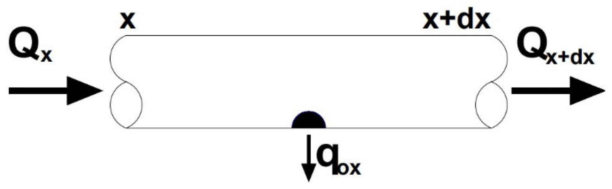
where q_o is the discharged flow rate, H is the pressure head at the orifice or emitter inlet, C_d is the discharge coefficient, and x is the emitter exponent. When the emitter is buried in the soil, the coefficient C_d also includes the orifice’s resistance and the soil around the pipe. Figure 1 shows an infinitesimal section of a drip lateral with length d_x. The water movement is regulated by the continuity and the motion equations.

$$Q_x=Q_{x+dx}+q_{ox}$$

(2)

$$A{V}_x=A{V}_{x+dx}+q_{ox}$$

(3)

where Q_x and Q_x+dx are the flow discharge at section x and x + d_x, q_ox is the emitter discharge at section x, A is the cross-sectional area of the lateral pipe, and V_x and V_x+dx are the flow velocity corresponding to Q_x and Q_x+dx, respectively.

Based on the equation of motion, the variation of pressure head between the sections x and x + dx of the lateral is given by:

$$H_x+\frac{V_x{}^2}{2g}=H_{x+dx}+\frac{V^2{}_{x+dx}}{2g}+dE+h_f$$

(4)

where H_x and H_x+dx are the pressure head at the sections x and x + dx, dE is the elevation difference that is due to the lateral slope S (positive for uphill and negative for downhill), h_f is the total head loss (friction and local losses), and g is the gravitational acceleration. The value of dE is given by:

$$dE=S.dx$$

(5)

The relationship between the flow velocity at the pipe section x, V_x, and the flow velocity at the section x + dx can be written as:

$$V_{x+dx}=V_x+\frac{\partial V_x}{\partial x}dx$$

(6)

Hence, considering that $H_{x+dx}=H_x+\frac{\partial H_x}{\partial x}dx$ and $h_f=\frac{\partial h_f}{\partial x}dx$, and substituting Equations (5) and (6) into Equation (4), it results in:

$$H_x+\frac{V_x{}^2}{2g}=H_x+\frac{\partial H_x}{\partial x}dx+\frac{1}{2g}(V_x{}^2+2V_x\frac{\partial V_x}{\partial x}dx+{(\frac{\partial V_x}{\partial x}dx)}^2)+Sdx+\frac{\partial h_f}{\partial x}dx$$

(7)

By neglecting the small quantities corresponding to the term ${(\frac{\partial V_x}{\partial x}dx)}^2$, the equation simplifies as:

$$\frac{\partial H_x}{\partial x}dx+\frac{V_x}{g}\frac{\partial V_x}{\partial x}dx+Sdx+\frac{\partial h_f}{\partial x}dx=0$$

(8)

The values of h_f can be evaluated with the Darcy–Weisbach equation:

$$h_f=\frac{f{V}_x^2}{2gD}{d}_x$$

(9)

where f is the dimensionless friction factor, d_x is the length of the pipe section, and D is the inner diameter of the lateral. As known, the friction factor f depends on the Reynolds number, R, and the pipe roughness. In smooth plastic pipes, the friction factor can be expressed with the Blasius or similar empirical equations [20].

To compute $\frac{\partial h_f}{\partial x}$, the implicit function theorem with respect to d_x was applied. Because d_x length is so small, the V_x and f variation are very small and negligible. In addition, the lateral diameter is constant and its variation is equal to zero. Therefore, the partial differential of the hf with respect to length is considered as $\frac{\partial h_f}{\partial x}$. By substituting from Equation (6) into Equation (3) and then into Equation (8) along with Equation (9), the continuity and the equations of motion result in:

$$A\frac{\partial V_x}{\partial x}dx+q_{ox}=0$$

(10)

$$\frac{\partial H_x}{\partial x}dx-\frac{V_x{q}_{ox}}{Ag}+Sdx+\frac{f{V}_x{}^2}{2gD}dx=0$$

(11)

By introducing λ = Ag/Vx and ω = (AgS/Vx + AfVx/2D) and explicating for q_ox, Equation (11) can be written as:

$$q_{ox}=\lambda \frac{\partial H_x}{\partial x}dx+\omega d_x$$

(12)

Two notes should be explained in Equation (12). First of all, as explained in Equation (1), the effect of soil resistance on emitter flow rate is included in the discharge coefficient, C_d. Therefore, the water discharged by buried emitters can be estimated from the pressure variations along the lateral. Second, when the distance between the emitters is small, the flow rate discharged by the lateral can be assumed as a linear source [21]. Moreover, when the pipe is horizontal or its slope is small, the term ωd_x can be neglected. In addition, because all the water discharged by the lateral reaches the soil, the rate of the water infiltration in the soil from the emitters has to be considered equal to the sum of the emitters discharge, q_ox. On the other hand, to identify the comprehensive model, Equation (12) has to be integrated into the soil moisture characteristic equation. Therefore, based on water mass volume change and considering that the water flowing in the soil from an area “a” around the buried emitters, we can write:

$$d{\theta }^{}a=q_{ox}dt=\lambda \frac{\partial H_x}{\partial x}d{x}^{}dt$$

(13)

To solve Equation (13), the value of “a” can be assumed constant and equal to the product of the distance between the emitters by half the circumference of the lateral. In the common conditions in a subsurface drip irrigation system using a drip line with small emitter spacing, in fact, the moisture at the beginning of the irrigation spreads rapidly in the soil and, after a short time, the wetting bulb around each emitter overlaps with that produced by the adjacent emitters. Finally, by introducing Equation (12) into Equation (13) and dividing for the area, it results in:

$$\frac{\partial \theta }{\partial t}=\frac{\lambda }{a}\frac{\partial H_x}{\partial x}dx$$

(14)

Equation (14) can be used to couple the lateral hydraulic parameters with the governing equation of soil and water movements, such as the Richards equation. Each of the two sides of this equation can be evaluated through the use of a specific computational program. The solution corresponding to the right side of Equation (14) has already been explained. To determine the value associated with the left side of the equation, the Richards equation should be solved based on the initial and boundary conditions. A three-dimensional numerical simulator is required to study the wetting fronts under the line source, such as the Hydrus-3D model, which can numerically solve the three-dimensional Richards equation for a line source [9,10]. Therefore, the Hydrus-3D model was chosen as a complementary section of the comprehensive model for the simulation of soil water infiltration and redistribution processes.

3. Materials and Methods

To assess the performance of the comprehensive model, the experimental components, including drip line hydraulic characteristics, soil texture, test pressures, and other test conditions were selected based on a set of common conditions of subsurface drip irrigation installation and operations. Therefore, the generated model can be used in other possible operating conditions.

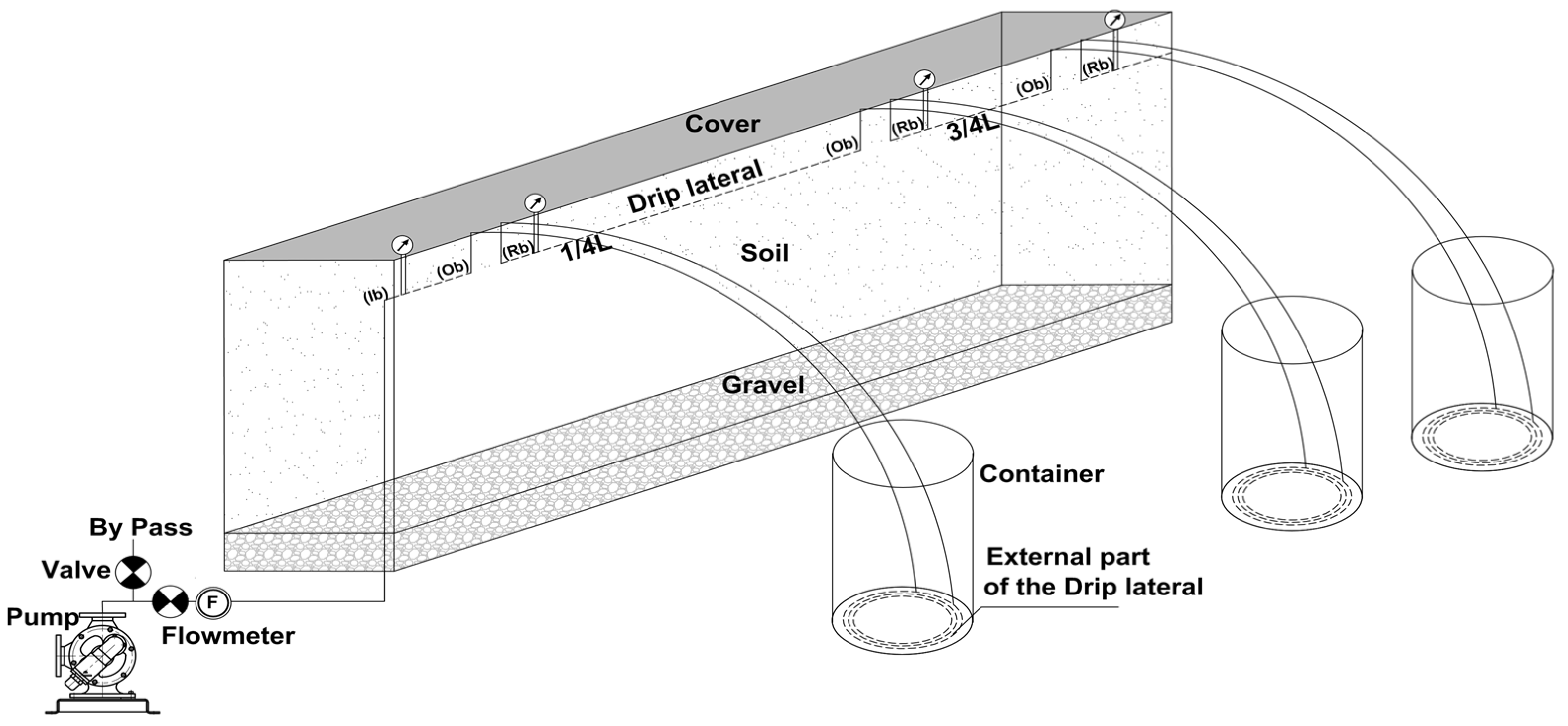
This study was conducted in an Isfahan municipality greenhouse in Iran (32°36′50″ N, 51°43′19″ E). The experiment was planned and carried out in a glass box with a size of 2 m × 0.4 m × 1.2 m (Figure 2), in which it was possible to control the initial and boundary conditions later used to run the Hydrus-3D model. Because all the sides of this soil box were transparent, the wetting patterns were visible during the experiment. The soil physical and hydraulic properties are presented in

Table 1. Soil physical and hydraulic properties.

Soil Properties	Sand (%)	Silt (%)	Clay (%)	Soil BD (gr/cm3)	Residual Water Content θr (cm3/cm3)	Saturated Water Content θs (cm3/cm3)	Shape Parameters			Saturated Hydraulic Conductivity Ks (cm/h)
							A (1/m)	n	l
Clay loam	36	31	33	1.57	0.08	0.41	1.34	1.37	0.5	0.3

.

Soil texture, bulk density, and saturated water content were directly measured through the laboratory methods and thereafter the water retention curve was gained by using the pressure plate apparatus for the pressures ranging from −33 to −1500 kPa. Then, the soil hydraulic parameters were optimized by running the Hydrus 3D inverse solution based on the soil water contents at the small part of the observation nodes measured at the pressure of one atmosphere for the drip line with 50 cm emitter spacing. This data was removed from the final model evaluation. The soil was sieved at 2 mm and packed in the soil box in 5 cm layers to prepare the experimental setup. Then, three samples of polyethylene pipe, with 16 mm nominal diameter and 62 m length, were used as subsurface drip irrigation drip laterals. These laterals contained co-extruded emitters whose flow rate ranged approximately from 2 to 5 L/h under different test pressures. The emitter spacings in the three pipes were 20, 40, and 50 cm. Considering that the distance between the emission points along the lateral pipes was less than 1 meter, the lateral pipe was supposed as a line source [21].

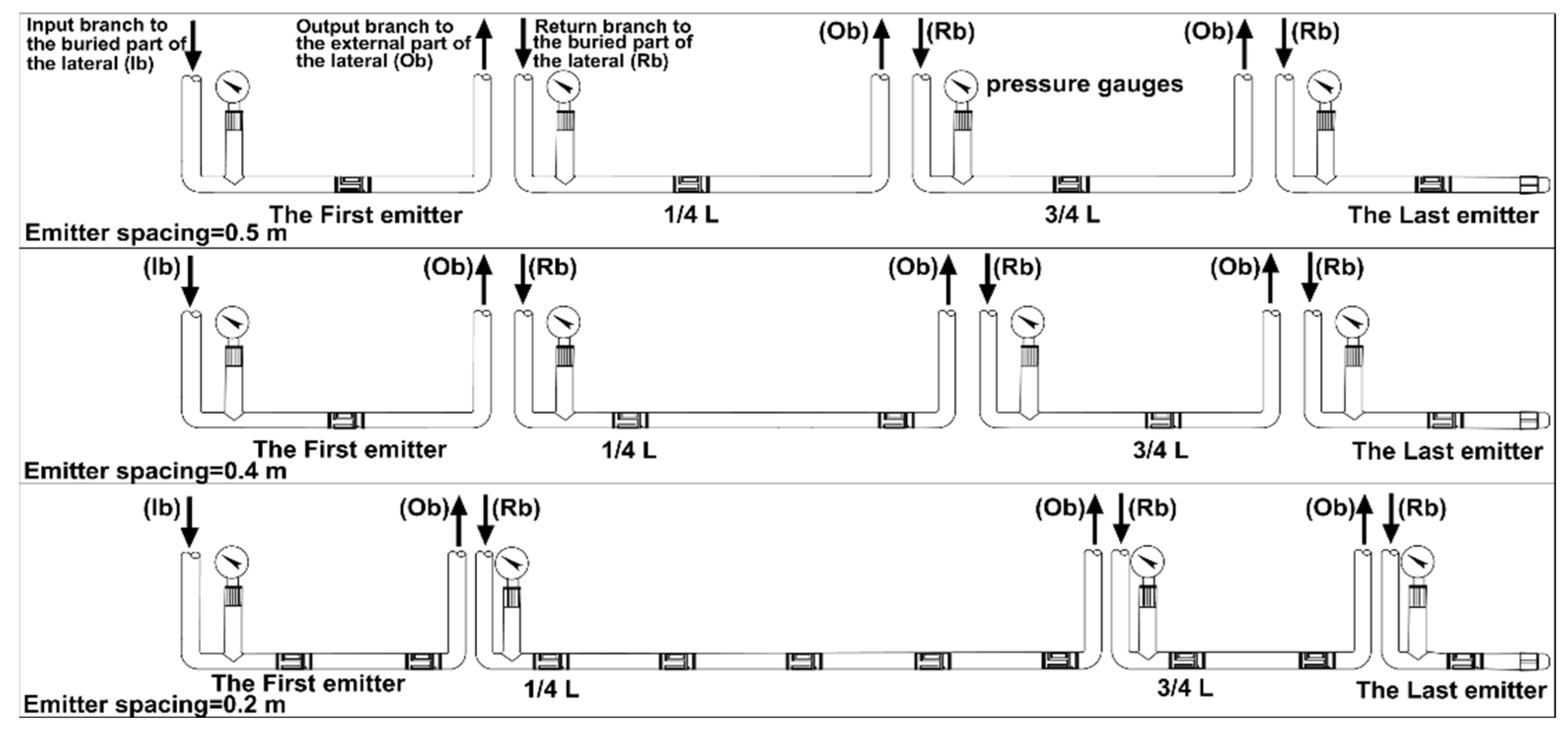
The governing relationship between the flow rate of the buried emitters and the pressure head was preliminarily determined through specific tests using the same hydraulic conditions occurring in the soil box to minimize unintended experimental errors. Four pressure gauges with a measurement accuracy of ±3% were installed in the hydraulic circuit: the first corresponded to the initial section of the buried pipe and the others beside the return branches next to the first quarter, fourth quarter, and the end of the lateral. Only 2 m of the lateral were buried into the soil box, whereas the other parts were removed from the soil box and put into three separate containers. The remaining lengths consisted of 15, 30, and 15 m of the drip lateral that were respectively installed outside the soil box (Figure 2). The portion of the lateral inside the box was installed at 20 cm depth, following its longitudinal wall, and connected to a pump and the other required tools such as bypass pipe, valves, flow meter, etc. Figure 3 shows a planar view of the input, output, return branches, and emitter positions in the buried part of the three drip laterals.

Operating pressures of 50, 100, and 150 kPa were applied by a pump and adjusted by a bypass valve. In all the experiments, the water temperature and the total suspended solids, TSS, were equal to 20 °C and 5 mg/L, respectively. All the experiments were carried out when the initial volumetric soil water content in the box was quite uniform and equal to 12%. To ensure the stability in the condition, water contents were measured in soil samples collected at 0, 20, and 40 cm away from the lateral and 20, 40, and 60 cm depths in the soil box before each experiment. The experiments related to the different drip laterals were carried out under the same explained condition in the soil box. The duration of each watering was 3 h, and the wetting pattern dimensions in two perpendicular planes were measured through the transparent walls of the container 1, 2, 3, and 24 h after the beginning of each experiment through photographs taken from the longitudinal and crosswise wetting patterns.

The soil moisture content in the area inside the wetting front is greater than the initial soil moisture content [22]. Therefore, a sampler was used to collect soil samples (with a minimum of 100 gr weight) in a soil volume of 20 cm × 20 cm × 20 cm around the emitter to determine the soil moisture distribution and the wetting pattern at the end of the experiments and 24 h after the beginning of each experiment. For determining the water volume infiltrated in the soil, the water volume discharged by the portions of pipe outside the soil box and collected into the containers was subtracted from the total volume measured with the flow meter.

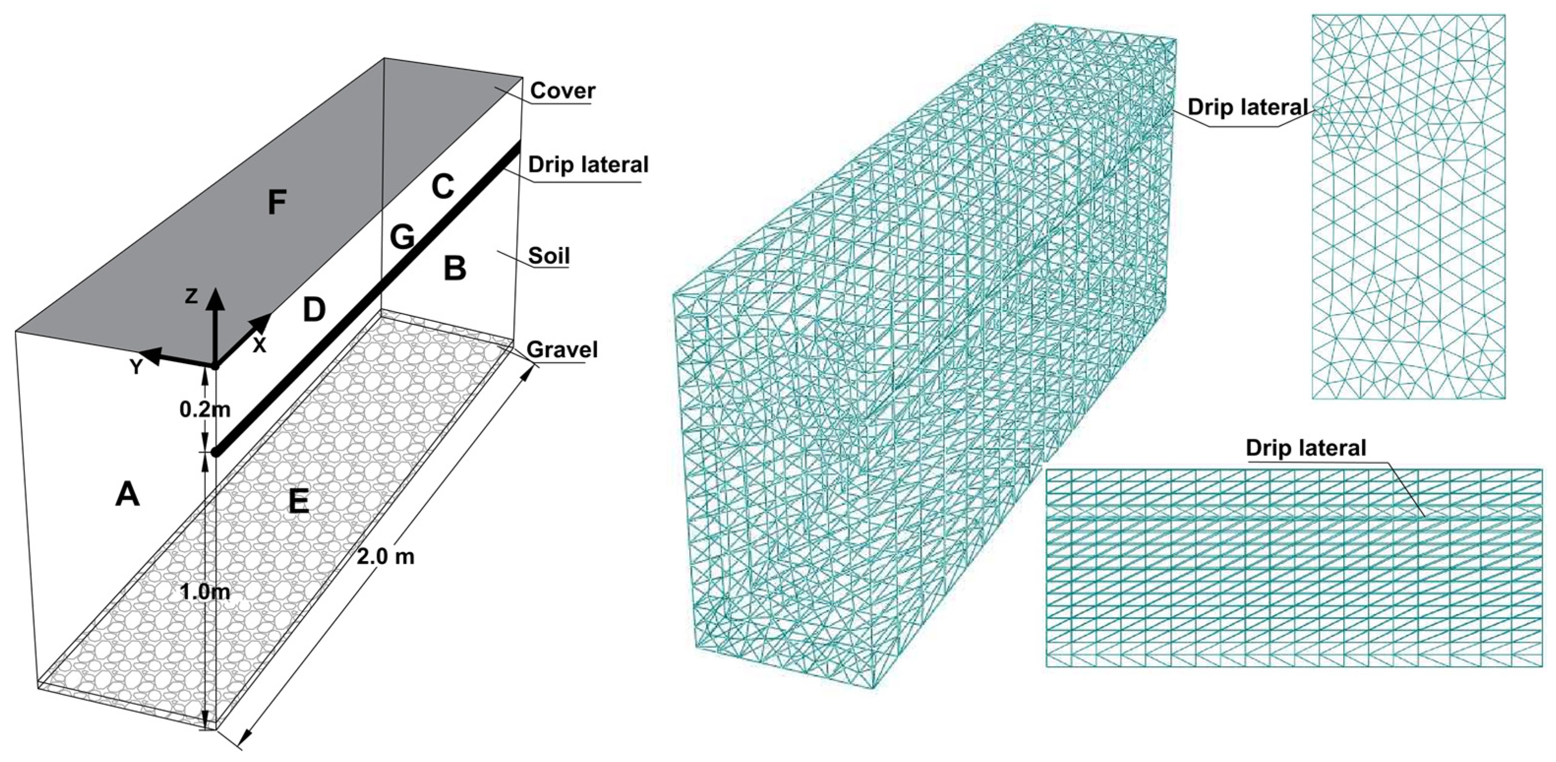
To run Hydrus-3D, it was necessary to discretize the flow domain according to a mesh. An unstructured triangular mesh was automatically generated with 4520 nodes for all the simulations. Figure 4 shows the soil box with the schematization of the grid and the subsurface drip irrigation lateral, as considered to run the Hydrus 3D model. Finite elements were smaller in the soil volume close to the upper boundary layer where the hydraulic gradient is higher and larger at increasing depth.

The smallest elements were located around the lateral and the size of the finite triangular elements became larger at increasing distances from the lateral.

The transport domain of the simulations, shown in Figure 4, was discretized with 50, 400, and 22,800 1D elements, 2D elements, and 3D elements, respectively. The comprehensive model can determine the pressure variation along the lateral by considering the available pressure head at the lateral inlet. Other geometrical and physical specifications, including the length, diameter, emitter spacing, emitters discharge, and ground slope, should be specified in the model input. Consequently, to perform the comprehensive model, a computer program developed in MATLAB was first applied to determine the pressure variations and flow fluxes along the lateral side. Then, the obtained fluxes with the other required parameters, including the soil hydraulic characteristics and the initial and boundary conditions were used as input to the HYDRUS-3D model to predict the wetting front dimensions along the pipe direction, as well as at the initial and final pipe sections.

The initial condition at t = 0 was assumed as:

$$\theta (x,y,z,t)={\theta }_0(x,y,z),(0<x<X,0<y<Y,0<z<Z,t=0);$$

(15)

For all the planes represented in Figure 4, the following boundary conditions were considered to reproduce the actual conditions observed in the soil box:

$$t>0, \frac{\partial h}{\partial z}=0, \mathrm{Plane} \mathrm{F};$$

(16)

$$t>0, \frac{\partial h}{\partial x}=\frac{\partial h}{\partial y}=0, \mathrm{Planes} \mathrm{A}, \mathrm{B}, \mathrm{C}, \mathrm{and} \mathrm{D};$$

(17)

$$t>0, \frac{\partial \theta }{\partial t}=\frac{\partial q_0}{\partial x}\ne 0, \mathrm{Surface} \mathrm{G};$$

(18)

$$t>0, \frac{\partial h}{\partial z}<0, \mathrm{Plane} \mathrm{E}.$$

(19)

4. Statistical Analysis

The accuracy and ability of the model to simulate the horizontal and vertical dimensions of the wetting front were assessed by using both the simulated and measured dimensions of the wetting zone, based on the mean absolute errors (MAE), the root mean square error (RMSE), and the refined index of agreement (dr) [23,24]:

$$MAE=\frac{1}{n}{\displaystyle \sum _{i=1}^n\left|(P_i-O_i)\right|}$$

(20)

$$RMSE=\sqrt{\frac{{\displaystyle \sum _{i=1}^n{(P_i-O_i)}^2}}{n}}$$

(21)

$$dr=\{\begin{array}{l}1-\frac{{\displaystyle \sum _{i=1}^n\left|P_i-O_i\right|}}{c{\displaystyle \sum _{i=1}^n\left|O_i-\overline{O}\right|}},when{\displaystyle \sum _{i=1}^n\left|P_i-O_i\right|}\le c{\displaystyle \sum _{i=1}^n\left|O_i-\overline{O}\right|}\\ \frac{c{\displaystyle \sum _{i=1}^n\left|O_i-\overline{O}\right|}}{{\displaystyle \sum _{i=1}^n\left|P_i-O_i\right|}}-1,when{\displaystyle \sum _{i=1}^n\left|P_i-O_i\right|}>c{\displaystyle \sum _{i=1}^n\left|O_i-\overline{O}\right|}\end{array}$$

(22)

where c is equal to two, O_i is the observed value, P_i is the predicted value, n is the number of observations, and Ō is the mean of the observed data. The dr index ranges from −1 to 1 and quantifies the prediction errors of the model relative to the observed deviations from the observed mean. Thus, a perfect agreement between data sets would result in dr = 1. In addition, the values of RMSE and MAE indices close to zero indicate an excellent performance for the model. In this study, RMSE, MAE, and dr values were applied to compare separately the soil wetted width and depth. For this purpose, the observed and predicted dimensions of the wetting front at the selected points have been determined. These points were intended at the first and last cross-sections of the lateral, as well as at 10 cm intervals along the longitudinal direction of the lateral.

5. Results and Discussion

The accurate estimation of the wetting front is one of the most effective factors for the optimal design and management of subsurface drip irrigation systems [10,25]. Therefore, in this study, the comprehensive model was developed and its performance verified. To investigate the model efficiency, the hydraulic analysis of the tested laterals was initially carried out, including the comparison between the water pressures measured by the manometers and the corresponding calculations by the model, based on the step-by-step procedure.

The results of the analysis for the different examined conditions are summarized in

Table 2. Summary of the hydraulic analysis results including the head losses, the measured (Hm) and estimated (He) pressure heads, their relative difference (RE), and the mean discharge of the buried emitters (q_o).

Emitter Spacing (cm)	Pressure (kPa)	50				100				150
	Selected Section	0	L/4	3L/4	L	0	L/4	3L/4	L	0	L/4	3L/4	L
50	Hf (m)	0.000	0.366	0.773	0.794	0.000	0.672	1.421	1.475	0.000	0.949	2.012	2.089
	He (m)	5.000	4.634	4.227	4.206	10.000	9.328	8.579	8.525	15.000	14.051	12.988	12.911
	Hm (m)	5.000	4.600	4.200	4.300	10.000	9.500	8.400	8.800	15.000	14.300	13.400	12.900
	RE (%)	0.000	0.739	0.643	2.186	0.000	1.811	2.131	3.125	0.000	1.741	3.075	0.085
	qo (l/h)	2.417	2.326	2.222	2.216	3.419	3.302	3.166	3.157	4.188	4.054	3.897	3.886
40	Hf (m)	0.000	0.547	1.146	1.186	0.000	0.792	1.907	1.983	0.000	1.436	2.994	3.100
	He (m)	5.000	4.453	3.854	3.814	10.000	9.208	8.093	8.017	15.000	13.564	12.006	11.900
	Hm (m)	5.000	4.500	4.050	4.000	10.000	9.500	8.200	7.900	15.000	13.700	11.900	11.700
	RE (%)	0.000	1.044	4.840	4.650	0.000	3.074	1.305	1.481	0.000	0.993	0.891	1.709
	qo (l/h)	2.417	2.281	2.124	2.113	3.419	3.281	3.076	3.061	4.188	3.983	3.747	3.730
20	Hf (m)	0.000	0.550	2.428	2.519	0.000	3.335	6.019	6.151	0.000	4.805	8.734	8.929
	He (m)	5.000	4.450	2.572	2.481	10.000	6.665	3.981	3.849	15.000	10.195	6.266	6.071
	Hm (m)	5.000	4.500	2.900	2.800	10.000	6.500	4.100	3.700	15.000	9.900	6.300	6.100
	RE (%)	0.000	1.111	11.310	11.393	0.000	2.538	2.902	4.027	0.000	2.980	0.540	0.475
	qo (l/h)	2.417	2.280	1.733	1.702	3.419	2.791	2.156	2.110	4.188	3.452	2.706	2.663

. For each tested emitter spacing and applied operating pressure at the lateral inlet, the values of head losses, the measured (H_m), and estimated (H_e) pressure heads, their relative difference (RE), as well as the mean discharge of the buried emitters corresponding to the emitters installed at 0, L/4, 3/4L, and L from the lateral inlet, are reported. To give an example, for the drip lines with 20 cm emitter spacing, the head loss between the emitter placed at a distance of 3/4L (46.4 m) from the lateral inlet and the upstream end of the lateral resulted in 2.428 m, 6.019 m, and 8.734 m under an applied pressure of 50, 100, and 150 kPa, respectively. A similar trend was also observed for the other examined cases. Moreover, for any fixed operating pressure, as a consequence of the pressure head reductions along the lateral even the flow rates discharged by the emitters decreased and the wetting profiles developed non-uniform patterns in the different sections of the laterals.

The hydraulic analysis of the lateral evidenced that the errors associated with the pressure head estimated by the model were generally lower than 5%, with an average value of about 2%. Maximum RE values of 3.125%, 4.84%, and 11.393% were obtained for drip laterals with 50, 40, and 20 cm emitter spacing, respectively, while the minimum values for the same three cases resulted in 0.085%, 0.891%, and 0.475%, respectively.

Considering that the emitter flow rate depends on the square root of the pressure head, the minor errors associated with the latter had no relevant effects on the emitter discharge. Therefore, the head losses along with the lateral were calculated step by step, accounting for the actual emitter discharge for model development. The model accuracy when determining the effective pressure heads on the emitters increased considerably and, consequently, the hydraulic section of the comprehensive model provided accurate estimations of water flux along the lateral and emitters’ outflow, whose values were used as the main input of the Hydrus 3D model to improve the performance of the simulations.

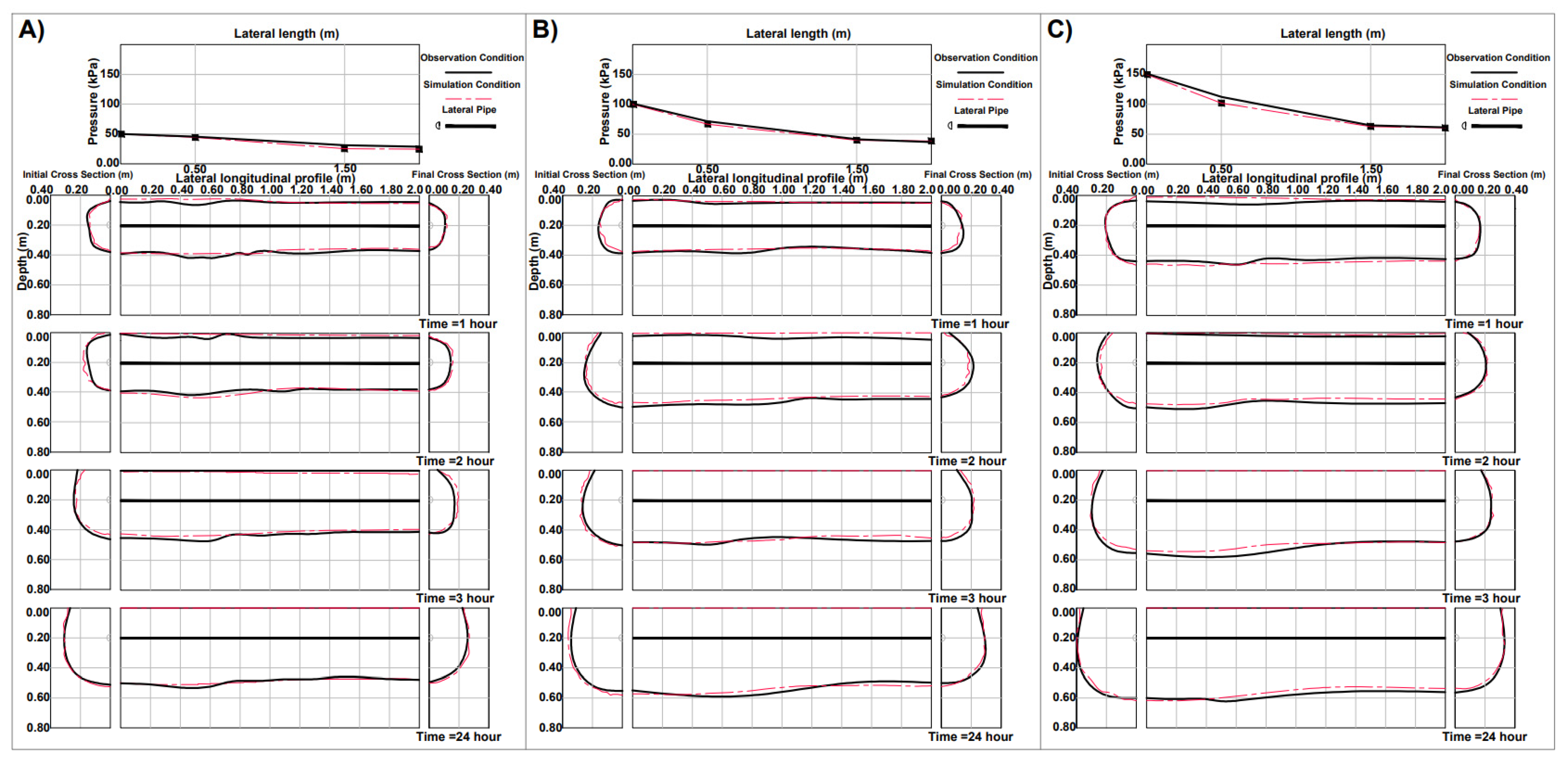
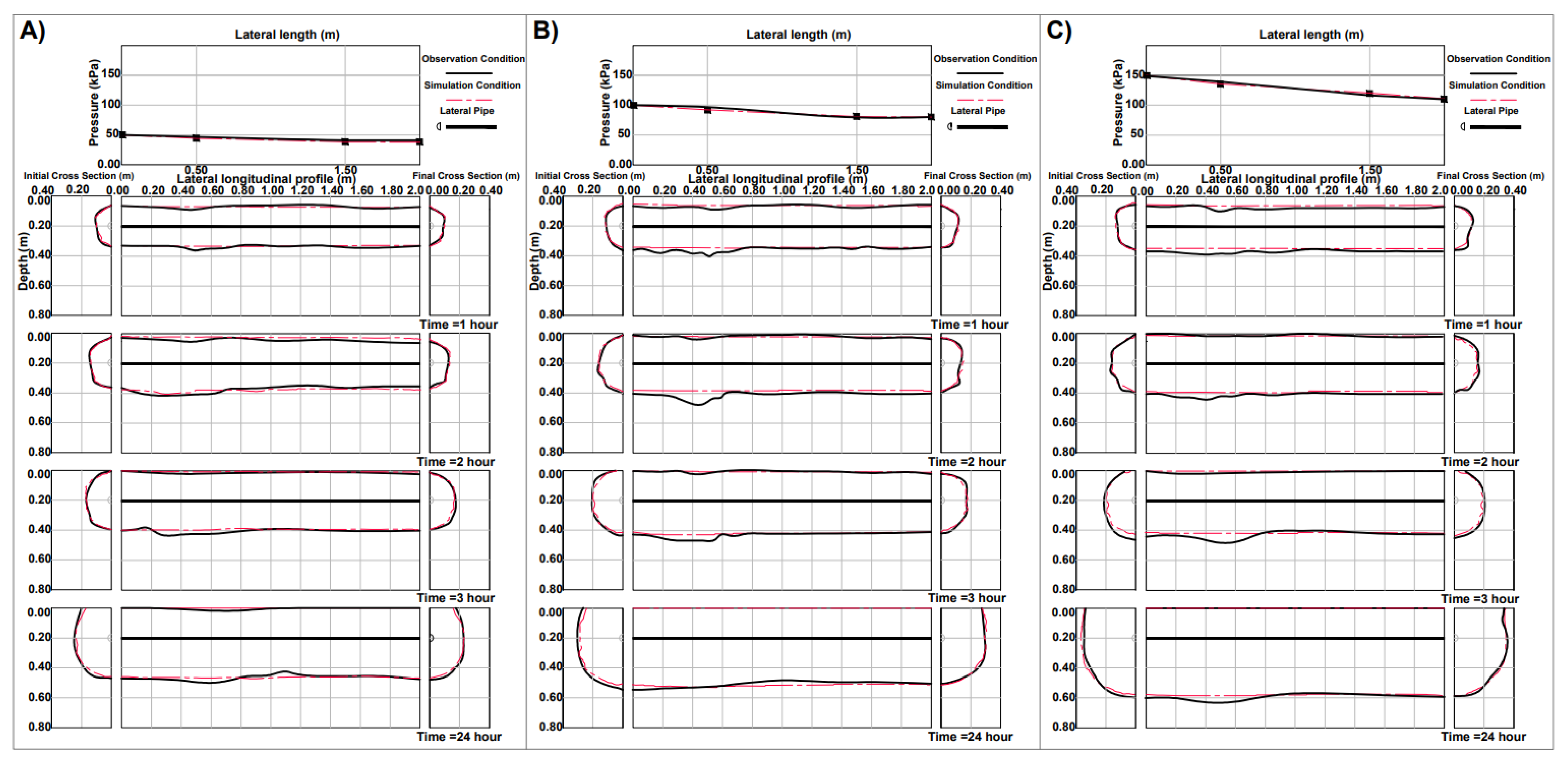
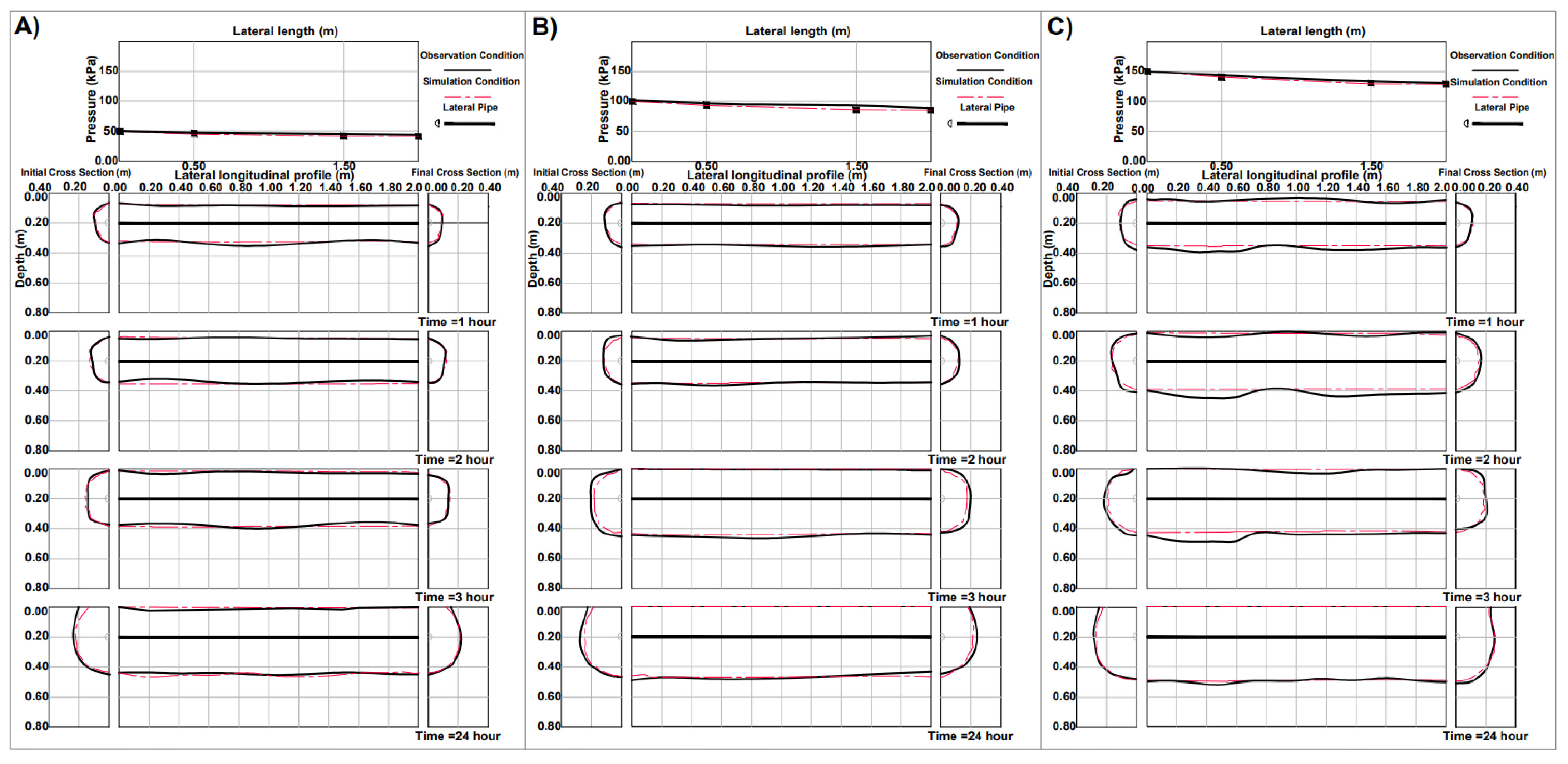
The observed and simulated wetting fronts, under the examined conditions, are shown in Figure 5, Figure 6 and Figure 7. Due to the negative slope of the energy gradient line, the water flux decreases along the flow direction. In fact, at increasing head losses, the effective pressure head on the emitters decreased, with the consequent reduction of the emitters’ outflow.

The volume of the water discharged in the soil container, the longitudinal wetted area along the lateral, and the transversal wetted area corresponding to the first and last cross-sections under the different examined conditions are summarized in

Table 3. Volumes of water discharged (V_w), the mean rate of the discharged water per emitter (q_sm), and wetted area measured along the longitudinal direction (A_L), initial (A_1C), and final (A_2C) cross-sections were obtained in all the experiments. The ratios between the discharged water to the wetted area are also indicated.

Operating Pressure (kPa)	Time-T (h)		1			2			3			24
	Emitter Spacing (cm)	50	40	20	50	40	20	50	40	20	50	40	20
50	VW (m3)	0.009	0.012	0.022	0.019	0.023	0.043	0.028	0.034	0.063	0.028	0.034	0.063
	qsm (l/h)	2.371	2.320	2.170	2.360	2.280	2.140	2.340	2.240	2.100	-	-	-
	AL (m2)	0.497	0.538	0.679	0.570	0.657	0.701	0.697	0.786	0.867	0.856	0.921	0.980
	VW/AL (m)	0.019	0.022	0.032	0.033	0.035	0.061	0.040	0.043	0.073	0.033	0.036	0.064
	A1C (m2)	0.021	0.023	0.042	0.028	0.040	0.046	0.054	0.052	0.097	0.080	0.099	0.137
	VW/A1C (m)	0.452	0.513	0.523	0.674	0.577	0.930	0.520	0.642	0.649	0.351	0.339	0.460
	A2C (m2)	0.018	0.018	0.030	0.029	0.030	0.040	0.047	0.052	0.060	0.086	0.095	0.107
	VW/A2C (m)	0.527	0.630	0.723	0.651	0.760	1.070	0.597	0.646	1.047	0.327	0.354	0.589
100	VW (m3)	0.013	0.017	0.034	0.026	0.033	0.066	0.039	0.048	0.095	0.039	0.048	0.095
	qsm (l/h)	3.320	3.300	3.400	3.280	3.250	3.300	3.220	3.220	3.150	-	-	-
	AL (m2)	0.537	0.574	0.684	0.625	0.782	0.870	0.886	0.891	0.936	0.933	1.011	1.075
	VW/AL (m)	0.025	0.029	0.050	0.042	0.042	0.076	0.044	0.054	0.101	0.041	0.048	0.088
	A1C (m2)	0.026	0.027	0.043	0.032	0.046	0.102	0.077	0.077	0.111	0.119	0.151	0.180
	VW/A1C (m)	0.511	0.623	0.791	0.820	0.710	0.647	0.502	0.626	0.851	0.325	0.320	0.525
	A2C (m2)	0.026	0.026	0.043	0.042	0.043	0.069	0.072	0.075	0.082	0.094	0.135	0.134
	VW/A2C (m)	0.511	0.635	0.789	0.625	0.756	0.952	0.540	0.642	1.148	0.411	0.358	0.705
150	VW (m3)	0.017	0.020	0.038	0.031	0.038	0.066	0.042	0.047	0.105	0.042	0.047	0.105
	qsm (l/h)	4.180	4.000	3.800	3.850	3.770	3.300	3.500	3.150	3.500	-	-	-
	AL (m2)	0.650	0.686	0.772	0.745	0.790	0.917	0.898	0.900	1.030	0.990	1.140	1.160
	VW/AL (m)	0.026	0.029	0.050	0.042	0.048	0.072	0.047	0.053	0.102	0.042	0.041	0.091
	A1C (m2)	0.029	0.032	0.052	0.038	0.048	0.104	0.081	0.079	0.136	0.120	0.181	0.220
	VW/A1C (m)	0.587	0.625	0.731	0.811	0.785	0.635	0.519	0.597	0.772	0.350	0.261	0.477
	A2C (m2)	0.028	0.029	0.053	0.050	0.051	0.070	0.072	0.077	0.100	0.113	0.160	0.163
	VW/A2C (m)	0.597	0.690	0.724	0.616	0.739	0.939	0.583	0.614	1.050	0.372	0.295	0.644

. For example, for the drip lateral with 20 cm emitter spacing after 24 h at the operating pressure of 150 kPa, the wetted area along the longitudinal direction and at the initial and final cross-sections were equal to 1.16, 0.22, and 0.163 m², respectively. These values were larger than the corresponding observed values in the experimental cases. On the contrary, the minimum wetted areas were 0.497, 0.021, and 0.018 m² after 1 h beneath the drip lateral with 50 cm emitter spacing at the operating pressure of 50 kPa.

The largest and smallest wetted area corresponded to the highest and the lowest discharged volumes, equal to 0.105 and 0.009 m³, respectively. The mean flow rates of the emitters in the mentioned cases varied from 2.1 to 4.18 L/h. Accordingly, at decreasing emitter spacing and increasing observation time and operating pressure, the wetted zone area and the ratio between the discharged water and the wetted area mostly increased. The results showed how the width and depth of the wetted zone increased with the emitter discharge rate. These results are in agreement with those presented by [5,26]. This phenomenon was observed even after the redistribution phase in the wetted longitudinal profiles, as well as in both cross-sections. The higher operating pressures, similar to the reductions of the emitter spacing, not only determined the increase of the discharged volume but also caused the expansion of the wetted bulb during both the distribution and redistribution processes.

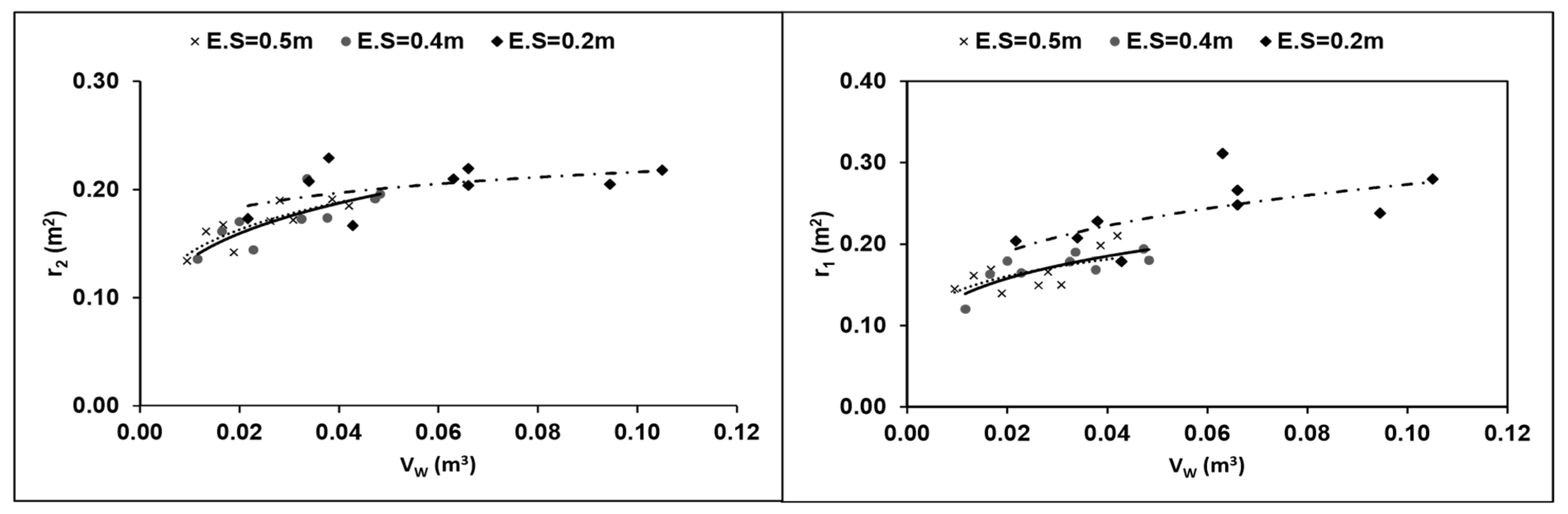
The results also proved that the diameter of wetted soil volume at initial (r₁) and final (r₂) cross-sections of the lateral with various emitter spacings (E.S) were related to the volume of water discharged (V_w) into the soil that is in agreement with the results of Thorburn et al. [27]; the diameter of wetted soil volume increased nonlinearly with applied water volume (Figure 8).

To evaluate the comprehensive model efficiency when simulating the wetting front dimensions, the model outputs were compared with the corresponding measured ones in each stage. To better investigate the results, soil water movement around the line source was divided into three time-steps. The first started from the beginning of the experiments and continued until the overlapping of wetted bulbs. The second lasted until the end of watering (3rd h) and the third, after the water redistribution process, lasted until the end of the experiments (24th h).

During the first stage of the infiltration process (when the soil is dry) overlapping of the wetting patterns between the emitters occurred earlier in the lateral with 20 cm emitter spacing compared to the other laterals with 40 cm and 50 cm emitter spacings. Similarly, in all of the examined drip lines, the increasing of the operating pressure determined the rise of the emitters’ discharges and the associated wetting front. These occurrences were a consequence of the closer distance between consecutive emitters, as well as of the dominant effect of the capillary on the gravity forces during the early stages of the infiltration process. Therefore, at first, the soil water content increased faster along the longitudinal direction (x-axis) compared to the transversal direction (y and z axes). In the following stage, the water moved in the radial direction. Accordingly, at the first stage of the soil– water distribution process, the comparison between simulated and measured wetting patterns confirmed that the sharper spreading wetting patterns occurred under the line source with higher water flux. In the second stage, after the overlap of the wetting front, a saturated layer formed around the lateral so that a positive pressure developed around the emitters. At this time, in line with the findings of Shani et al. [28], the emitter discharge reduced so that the total flow rate of the lateral, measured by the flow meter, decreased. In this situation, the capillary effect on the spreading wetted zone was negligible. Consequently, the mechanism of soil moisture distribution changed and the moisture mostly depleted from the saturated layer around the lateral to the neighboring area. Hence, at this stage, the rates of water movement and the spreading wetting front decreased. Similar to the Elmaloglou and Diamantopoulos [13] results, higher soil water content around the lateral was observed at relatively higher water fluxes; however, in contrast with their results, larger dimensions of wetting patterns resulted from additional water flux. As shown in Figure 5, particularly for the drip line with 20 cm emitter spacing, the observed and simulated wetting patterns followed the test pressure and the increasing water flux determined the expansion of the wetted zone.

In the third stage, after the end of watering, the redistribution process was also evaluated. Due to the different emitter spacing and flow rates, the volume of water discharged into the soil from each lateral resulted in being quite different from the other ones. Therefore, the water accumulated in wetted layers close to the laterals was gradually redistributed to the surrounding volume and increased the wetting front area beneath the lateral. Of course, relatively higher water flux applied during watering caused larger dimensions of the wetted zone. Both the model simulations and the experimental results indicated that the wetted area was greater during the redistribution process (stage three) than in the other stages. Moreover, even downward infiltration was greater than the corresponding upward. Figure 5, Figure 6 and Figure 7 indicated that the upper borders of the wetting patterns remained approximately at 6 ± 1 cm depth from the soil surface; soil wetting was not observed on the soil surface in the first hour of all the experiments. It can be argued that at the beginning of the tests, the upward moisture movement was affected by the capillary forces. Therefore, the water accumulated close to the lateral tended to move in the direction of minimum resistance after the merging of the wetting front. As indicated above, upward wetted soil developed faster immediately after the saturation of the soil around the lateral. Figure 5, Figure 6 and Figure 7 indicate that the wetted longitudinal profiles were uniform at the early times of the experiments, mainly during the first and second stages. Nevertheless, the continuity of further water flux in the first part of the lateral resulted in non-uniform water distribution through the soil, particularly at the end of the third stage. Additionally, the statistical parameters, including MAE, RMSE, and dr indices, were calculated to assess the model’s ability to predict the wetted profiles around buried laterals, as well as the cross-sections at the beginning and the end of the lateral. The summary of the statistical parameters in the different experiments is presented in

Table 4. Mean absolute errors (MAE), the root mean square error (RMSE), and the refined index of agreement (dr) indices obtained when comparing the observed and predicted wetted areas in the longitudinal and transversal flow directions.

	The Wetted Area around the Buried Lateral
Emitter Spacing	Mean Absolute Errors (m)			Root Mean Square Error (m)			Refined Index of Agreement
	50 kPa	100 kPa	150 kPa	50 kPa	100 kPa	150 kPa	50 kPa	100 kPa	150 kPa
20 cm	0.002	0.003	0.004	0.015	0.020	0.024	0.913	0.918	0.924
40 cm	0.002	0.002	0.004	0.013	0.020	0.030	0.920	0.921	0.902
50 cm	0.002	0.002	0.004	0.015	0.013	0.027	0.924	0.927	0.886
	Initial and final cross-sections of the lateral
20 cm	0.003	0.004	0.002	0.020	0.020	0.020	0.912	0.814	0.914
40 cm	0.001	0.003	0.002	0.011	0.035	0.014	0.937	0.876	0.939
50 cm	0.001	0.003	0.001	0.014	0.021	0.012	0.942	0.919	0.921

.

Based on Table 4, MAE values ranged from 0.001 to 0.004 m and RMSE values varied from 0.011 to 0.035 m. In addition, the minimum and maximum values of the dr were 0.814 and 0.942, respectively. Hence, the refined index of agreement values of the proposed model is fairly close to one. In addition, low RMSE values indicate that simulated values are very similar to the measured ones. Therefore, even the statistical analysis revealed that the differences between measured and predicted values of the wetting dimensions are quite negligible.

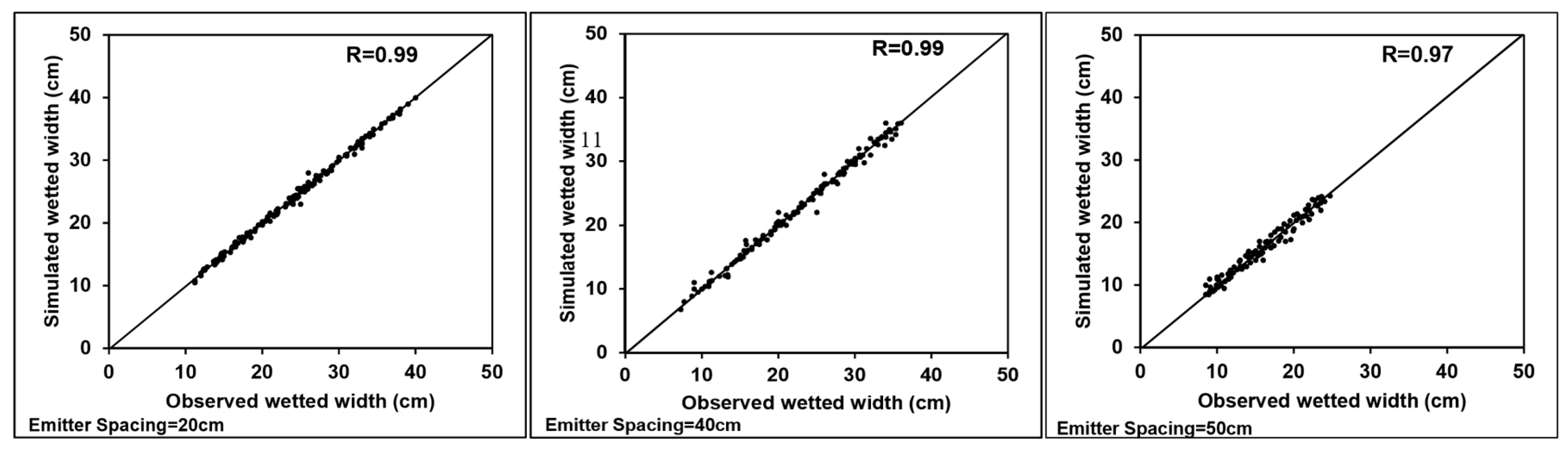
Figure 9 illustrates the comparison between observed and predicted wetted width at the first and last cross-sections of the laterals with emitter spacing of 20, 40, and 50 cm.

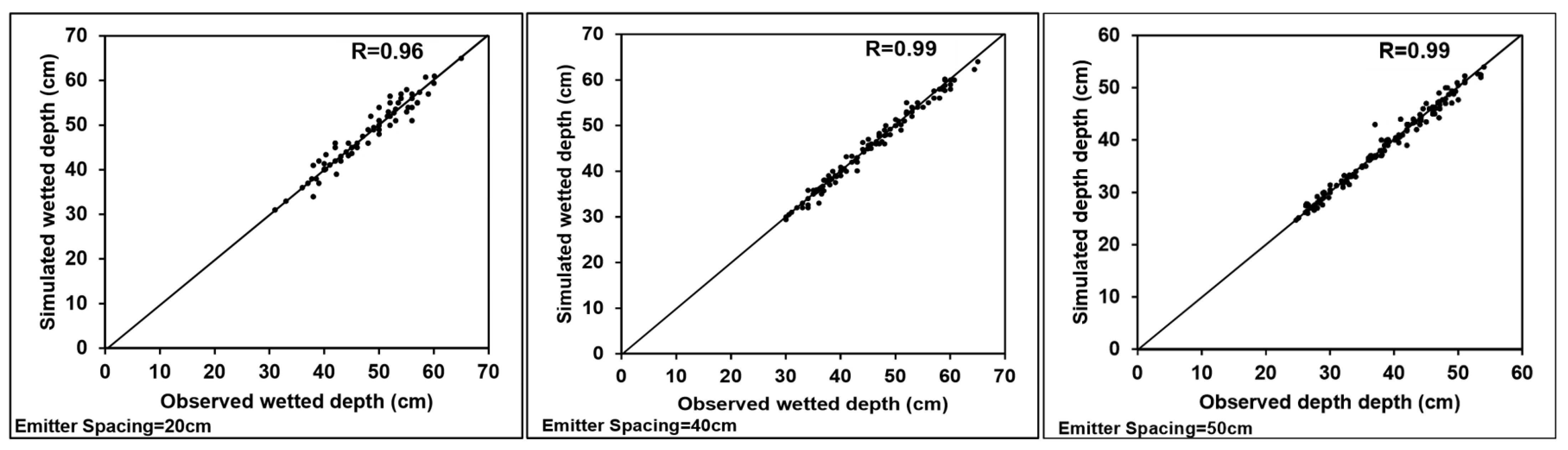
Similarly, Figure 10 shows the comparison between observed and predicted wetted depth obtained under the different operating pressures at distances of 0, L/4, 3L/4, and L from the upstream end of the laterals during both the water distribution and redistribution processes. As shown in Figure 9, the simulated values closely and homogeneously cluster around the 1:1 line. In addition, even based on Figure 10, the simulated wetted depths in all the examined cases were very close to the observed ones. Moreover, the values of the correlation coefficient in all the charts are positive and approximately close to +1, which indicates that the simulated values have perfect positive correlation with observed values and so relationships between the simulated and observed values are very close and both variables move in the same direction together.

Finally, it can be concluded that the comprehensive model provided a good estimation of the emitters’ outflows and represented realistic wetting fronts in all the stages of the experiments.

6. Conclusions

Based on the good agreement between the observed and model-simulated values for both the emitter flow rates and the wetting front dimensions, the comprehensive model can be considered reliable, useful, and efficient for estimating the variability of the emitter discharge and the wetting patterns throughout the soil profile in which a subsurface drip irrigation lateral is buried. The proposed model has several advantages over the existing models. First of all, the reduction of the emitter’s outflow because of the positive water pressure in the cavity around the emitter is accounted for in the discharge coefficient of the emitter flow rate-pressure head relationship. Second, instead of calculating the total head loss along the lateral using the discharge reduction coefficient, the model can determine the actual pipe friction losses in each lateral section. This model does not require any assumptions to be made for the lateral pressure analysis, as normally applied in other models (equal emitter discharge and/or discharge reduction coefficient). Finally, the good agreement between the simulated and observed dimensions of the wetting front also proved the good performance of the model outcomes during both the water distribution and redistribution processes.

Consequently, the comprehensive model can provide an accurate prediction of the wetting patterns around a buried SDI system lateral using easily accessible hydraulic parameters of the buried lateral and soil properties. Therefore, applying this model can improve the design accuracy and optimize the water management and consequently reduce the losses of water, fertilizer, and nutrients.

On the basis of the promising findings presented in this paper, it is recommended to apply and evaluate the model performance in field conditions.

References

- Schwartzman, M.; Zur, B. Emitter spacing and geometry of wetted soil volume. J. Irrig. Drain. Eng. 1986, 112, 242–253. [Google Scholar] [CrossRef]
- Warrick, A.; Lomen, D.; Amoozegar-Fard, A. Linearized moisture flow with root extraction for three dimensional, steady conditions. Soil Sci. Soc. Am. J. 1980, 44, 911–914. [Google Scholar] [CrossRef]
- Shiri, J.; Karimi, B.; Karimi, N.; Kazemi, M.H.; Karimi, S. Simulating wetting front dimensions of drip irrigation systems: Multi criteria assessment of soft computing models. J. Hydrol. 2020, 585, 124792. [Google Scholar] [CrossRef]
- Simunek, J. Models of water flow and solute transport in the unsaturated zone. Encycl. Hydrol. Sci. 2006. [Google Scholar] [CrossRef]
- Singh, D.; Rajput, T.; Sikarwar, H.; Sahoo, R.; Ahmad, T. Simulation of soil wetting pattern with subsurface drip irrigation from line source. Agric. Water Manag. 2006, 83, 130–134. [Google Scholar] [CrossRef]
- Cook, F.J.; Thorburn, P.J.; Fitch, P.; Bristow, K.L. WetUp: A software tool to display approximate wetting patterns from drippers. Irrig. Sci. 2003, 22, 129–134. [Google Scholar] [CrossRef]
- Bouchemella, S.; Seridi, A.; Alimi-Ichola, I. Numerical simulation of water flow in unsaturated soils: Comparative study of different forms of Richards equation. Eur. J. Environ. Civ. Eng. 2015, 19, 1–26. [Google Scholar] [CrossRef]
- Elmaloglou, S.; Malamos, N. A method to estimate soil-water movement under a trickle surface line source, with water extraction by roots. Irrig. Drain. J. Int. Comm. Irrig. Drain. 2003, 52, 273–284. [Google Scholar] [CrossRef]
- Honari, M.; Ashrafzadeh, A.; Khaledian, M.; Vazifedoust, M.; Mailhol, J. Comparison of HYDRUS-3D soil moisture simulations of subsurface drip irrigation with experimental observations in the south of France. J. Irrig. Drain. Eng. 2017, 143, 04017014. [Google Scholar] [CrossRef] [Green Version]
- Kandelous, M.M.; Simunek, J.; Van Genuchten, M.T.; Malek, K. Soil water content distributions between two emitters of a subsurface drip irrigation system. Soil Sci. Soc. Am. J. 2011, 75, 488–497. [Google Scholar] [CrossRef]
- Karandish, F.; Simunek, J. A comparison of the HYDRUS (2D/3D) and SALTMED models to investigate the influence of various water-saving irrigation strategies on the maize water footprint. Agric. Water Manag. 2019, 213, 809–820. [Google Scholar] [CrossRef] [Green Version]
- Sakaguchi, A.; Yanai, Y.; Sasaki, H. Subsurface irrigation system design for vegetable production using HYDRUS-2D. Agric. Water Manag. 2019, 219, 12–18. [Google Scholar] [CrossRef]
- Elmaloglou, S.; Diamantopoulos, E. Simulation of soil water dynamics under subsurface drip irrigation from line sources. Agric. Water Manag. 2009, 96, 1587–1595. [Google Scholar] [CrossRef]
- Hathoot, H.M.; Al-Amoud, A.I.; Mohammad, F.S. Analysis and design of trickle-irrigation laterals. J. Irrig. Drain. Eng. 1993, 119, 756–767. [Google Scholar] [CrossRef]
- Holzapfel, E.A.; Mario, M.A.; Valenzuela, A. Drip irrigation nonlinear optimization model. J. Irrig. Drain. Eng. 1990, 116, 479–496. [Google Scholar] [CrossRef]
- Warrick, A.; Yitayew, M. Trickle lateral hydraulics. I: Analytical solution. J. Irrig. Drain. Eng. 1988, 114, 281–288. [Google Scholar] [CrossRef]
- Kang, Y.; Nishiyama, S. Analysis and design of microirrigation laterals. J. Irrig. Drain. Eng. 1996, 122, 75–82. [Google Scholar] [CrossRef]
- Rodríguez-Sinobas, L.; Gil, M.; Juana, L.; Sánchez, R. Water distribution in laterals and units of subsurface drip irrigation. I: Simulation. J. Irrig. Drain. Eng. 2009, 135, 721–728. [Google Scholar] [CrossRef]
- Ren, C.; Zhao, Y.; Dan, B.; Wang, J.; Gong, J.; He, G. Lateral hydraulic performance of subsurface drip irrigation based on spatial variability of soil: Experiment. Agric. Water Manag. 2018, 204, 118–125. [Google Scholar] [CrossRef]
- Bagarello, V.; Ferro, V.; Provenzano, G.; Pumo, D. Experimental study on flow-resistance law for small-diameter plastic pipes. J. Irrig. Drain. Eng. 1995, 121, 313–316. [Google Scholar] [CrossRef]
- Lamm, F.R.; Ayars, J.E.; Nakayama, F.S. Microirrigation for Crop Production: Design, Operation, and Management; Elsevier: Amsterdam, The Netherlands, 2006. [Google Scholar]
- Bresler, E.; Heller, J.; Diner, N.; Ben-Asher, I.; Brandt, A.; Goldberg, D. Infiltration from a trickle source: II. Experimental data and theoretical predictions. Soil Sci. Soc. Am. J. 1971, 35, 683–689. [Google Scholar] [CrossRef]
- Nash, J.E.; Sutcliffe, J.V. River flow forecasting through conceptual models part I—A discussion of principles. J. Hydrol. 1970, 10, 282–290. [Google Scholar] [CrossRef]
- Willmott, C.J. Some comments on the evaluation of model performance. Bull. Am. Meteorol. Soc. 1982, 63, 1309–1313. [Google Scholar] [CrossRef] [Green Version]
- Cote, C.M.; Bristow, K.L.; Charlesworth, P.B.; Cook, F.J.; Thorburn, P.J. Analysis of soil wetting and solute transport in subsurface trickle irrigation. Irrig. Sci. 2003, 22, 143–156. [Google Scholar] [CrossRef]
- Liu, Z.; Li, P.; Hu, Y.; Wang, J. Wetting patterns and water distributions in cultivation media under drip irrigation. Comput. Electron. Agric. 2015, 112, 200–208. [Google Scholar] [CrossRef]
- Thorburn, P.J.; Cook, F.J.; Bristow, K.L. Soil-dependent wetting from trickle emitters: Implications for system design and management. Irrig. Sci. 2003, 22, 121–127. [Google Scholar] [CrossRef]
- Shani, U.; Xue, S.; Gordin-Katz, R.; Warrick, A. Soil-limiting flow from subsurface emitters. I: Pressure measurements. J. Irrig. Drain. Eng. 1996, 122, 291–295. [Google Scholar] [CrossRef]
Figure 1.
Elemental section of a drip lateral having length dx and with one emitter.
Figure 2.
Schematic view of the experimental setup.
Figure 3.
Planar view of the input, output, return branches, and the emitter positions in the buried part of the three drip laterals at the 0.2 m depth in the soil box.
Figure 4.
Finite element representation of the soil box and schematization of the lateral.
Figure 5.
Comparison between observed and simulated wetting fronts for drip lateral with 20 cm emitter spacing at operating pressures of (A) 50 kPa, (B) 100 kPa, and (C) 150 kPa.
Figure 6.
Comparison between observed and simulated wetting fronts for drip lateral with 40 cm emitter spacing at operating pressures of (A) 50 kPa, (B) 100 kPa, and (C) 150 kPa.
Figure 7.
Comparison between observed and simulated wetting fronts for drip lateral with 50 cm emitter spacing at operating pressures of (A) 50 kPa, (B) 100 kPa, and (C) 150 kPa.
Figure 8.
Relationship between the radiuses of the first and last cross-sections (r1&r2) and volume of water discharged (Vw) of the drip laterals with emitter spacing of 20, 40, and 50 cm.
Figure 9.
Simulated vs. observed wetted width at the first and last cross-sections of drip laterals with emitter spacing of 20, 40, and 50 cm.
Figure 10.
Simulated vs. observed wetted depth obtained at distances of 0, L/4, 3L/4, and L from the upstream section of the laterals with emitter spacing of 20, 40, and 50 cm.