
A Simplified Method for Leakage Estimation of Clay Core Dams with Different Groundwater Levels


1
State Key Laboratory of Hydrology-Water Resources and Hydraulic Engineering, Hohai University, Nanjing 210098, China
2
The College of Water Conservancy and Hydropower Engineering, Hohai University, Nanjing 210098, China
*
Author to whom correspondence should be addressed.
Water 2022, 14(12), 1961; https://doi.org/10.3390/w14121961
Submission received: 31 May 2022
/
Revised: 16 June 2022
/
Accepted: 17 June 2022
/
Published: 19 June 2022
(This article belongs to the Special Issue Safety Monitoring and Management of Reservoir and Dams)
Abstract
:Clay core dams are widely applied in reservoir construction, regulating water resource and provide electric power. Leakage is a common problem in reservoir construction, and the leakage amount, which not only affects the economic benefits of the project, but also relates to the safety of the dam body, is difficult to estimate. According to Darcy’s law and stable seepage theory, an analytical method can be proposed to calculate the leakage of the clay core dam to gain the seepage flux in a short time. By making some reasonable assumptions, we propose formulae for seepage calculation in different conditions of the position of the groundwater levels, below or above the reservoir bottom. Both sets of formulae contain two parts of leakage calculation, i.e., leakage from the reservoir bottom and leakage from the dam body. By using the proposed analytical method, the leakage of clay core dams can be estimated considering the influence of the groundwater level. To prove the rationality of the analytical method, a simple numerical model can be established using Geo-studio 2020 to calculate the seepage flux of the clay core dam, where relative errors between numerical solutions and analytical solutions are less than 10%. To verify the feasibility in engineering applications, the proposed method was applied to calculate the seepage of a clay core dam in Sichuan, China, which was also calculated using numerical methods by establishing a three-dimensional model. The results show the rationality of the analytical method, which can strike a balance between precision and efficiency.
1. Introduction
A clay core dam is a special kind of earth rock dam which has a long history and is widely used in hydraulic engineering to regulate water resources and provide electric power [1,2]. The dam body is made of local materials, with low transportation costs, a simple structure, and a long service life. Different from a homogeneous dam, a clay core dam is equipped with a special impervious core in the dam body, which uses sand and stone with high permeability as the dam shell, and the impervious core adopts cohesive soil with good impervious performance. In the normal operation of the clay core dam, leakage problems endanger the hydraulic engineering in many aspects [3,4,5,6,7]. Some serious leakage problems even result in dam breakage due to a variety of mechanisms such as fracturing and collapse [8]. The Mostiště embankment dam, the first compacted rockfill dam with a relatively thin inclined impervious core in the Czech Republic, was troubled by seepage problems 36 years after its completion. The defects could not be determined due to the lack of a drainage and seepage observation system. The leakage problem worsened, and at the end of 2004, the reservoir level was significantly lowered, threatening the life and property safety of downstream residents [9]. Internal erosion in embankment dams, which leads to ageing effects and further causes dam failures, accidents, and deterioration of dams, is still not a completely understood phenomenon. Mattsson et al. [10] developed a numerical model that can capture the processes of internal erosion in a physically sound fashion in the simulation, and the method may become a tool for future improvements regarding dam safety issues. Many scholars have conducted research on leakage problems of reservoirs. A seepage measurement system is an important part of a dam monitoring system. Temperature and resistivity measurements are two methods for seepage monitoring of embankment [11,12,13]. The identification of singularities with increased leakage can be performed using various techniques. Ghafoori et al. [14] reviewed the different techniques of DTS measurement calibration and the interpretation methods of temperature data. These techniques are all helpful in seepage monitoring, but before the project construction, they cannot help estimate the leakage amount, based on which proper measures can be taken to reduce the leakage amount and maintain the safe operation of the project. To estimate the leakage amount of a clay core dam during the design stage, effective methods should be strategized.
There are two main methods for seepage calculation of the clay core dam, i.e., numerical methods and analytical methods. Numerical methods were first employed to calculate the seepage flux several decades age [15], and have developed rapidly since the improvement of computer performance in recent years. Usually, there are three main numerical methods for seepage simulation, namely, the finite element method (FEM) [16,17,18,19], the finite difference method (FDM) [20,21,22], and the boundary element method (BEM) [23,24,25,26]. Aldulaimi [16] adopted a numerical approach utilizing FEM to simulate the seepage field of an earthfill dam, and the approach was used to carry out seepage analysis on an earth dam in Iraq. Salmasi et al. [17] established numerical models to simulate the seepage field of clay core dams and compared the performance of dams with a vertical core and with an inclined core. Li et al. [18] applied ABAQUS to calculate the seepage discharge of earth-rock dams under different conditions, based on which the phreatic line can be obtained. Elkamhawy et al. [19] established a two-dimensional steady state model to calculate the leakage amount of the Ismailia canal and assessed the anti-seepage effect of lining. Smith et al. [27] calibrated a numerical simulation tool, which can be widely used for seepage analysis. Beiranvand and Komasi [28] investigated the anti-seepage effects of the cut-off wall of the Eyvashan earth dam based on the numerical solutions and the experimental results. In recent times, research involving soft computing methods has been carried out to establish seepage parameters [29]. There are numerous recent studies on seepage modeling using soft computing methods. For example, based on recorded data, Parsaie et al. [30] used soft computing models to estimate the phreatic line and discharge of dams. These studies can help solve leakage problems and have guiding significance for the construction and operation of hydraulic engineering. However, it often takes substantial time to establish numerical models. It is difficult to gain seepage flux information within a short time despite the accuracy of numerical methods.
Another main way to estimate leakage is the use of analytical methods, which are more time-saving and convenient compared to numerical methods. Seepage flux information can be obtained quickly when the requirement for accuracy is relatively low. To solve seepage problems using analytical methods, it is important to establish acceptable simplifications and relevant boundary conditions [31,32,33,34,35]. Many well-known researchers studied analytical solutions to seepage through embankments, including Pavlovsky [36], Dachler [37], Davison and Rosenhead [38], Casagrande [39], Nelson-Skornyakov [40], and Aravin and Numerov [41,42]. These “old” models can be used to calculate the seepage flux and the phreatic line by assuming the cross-section of the dam to be a homogeneous entity. Mao [43] summarized the common seepage problems in hydraulic engineering and proposed a series of analytical methods for seepage calculation in various hydraulic structures based on the above “old” models. In recent years, Kacimov et al. [44,45,46] researched analytical solutions concerning seepage through clay core dams. An analytical calculation study was conducted on seepage through a zoned clay core dam, where the flow rate and phreatic surface were calculated [44]. Kacimov and Obnosov [45] analyzed the seepage of a clay core dam with a core of relatively low permeability, and further investigated the transition characteristics of seepage in different regions. Numerical solutions were used to compare with the analytical solutions, showing that analytical and numerical solutions are consistent in case of minor soil capillarity [46]. Rezk [47] developed an analytical solution to investigate the effect of core with different permeability levels on seepage flow and phreatic line position. Fakhari and Ghanbari [48] studied many numerical models of clay core dams to develop new approximate equations for seepage calculation and gained relatively high precision. Additionally, seepage through cores may be also obtained using velocity hodographs [45]. These studies have helped in obtaining seepage flux through the dam body, but ignore the leakage of water from the reservoir bottom and periphery, which are important parts of the total leakage. Additionally, the influence of different groundwater levels on the leakage amount is not considered.
In order to make the engineering design process quicker and more targeted, analytical methods should be applied to calculate the leakage amount of the clay core dam. By simplifying the calculation process, engineers can gain results in a short time to assess the engineering safety and economy. In this research, by making some reasonable assumptions, an analytical method is proposed for the seepage calculation of the clay core dam (including the dam body and the reservoir bottom). According to Darcy’s law and stable seepage theory, two sets of formulae are proposed for seepage calculation of the clay core dam in different conditions of the position of the groundwater levels. A simple numerical model was built to calculate the seepage flux of the clay core dam using Geo-studio 2020 software to verify the rationality of the formulae. At last, the simplified method was used for leakage calculation of a clay core dam in Sichuan, China, which demonstrates its feasibility in engineering applications.
2. Method
2.1. Basic Assumptions
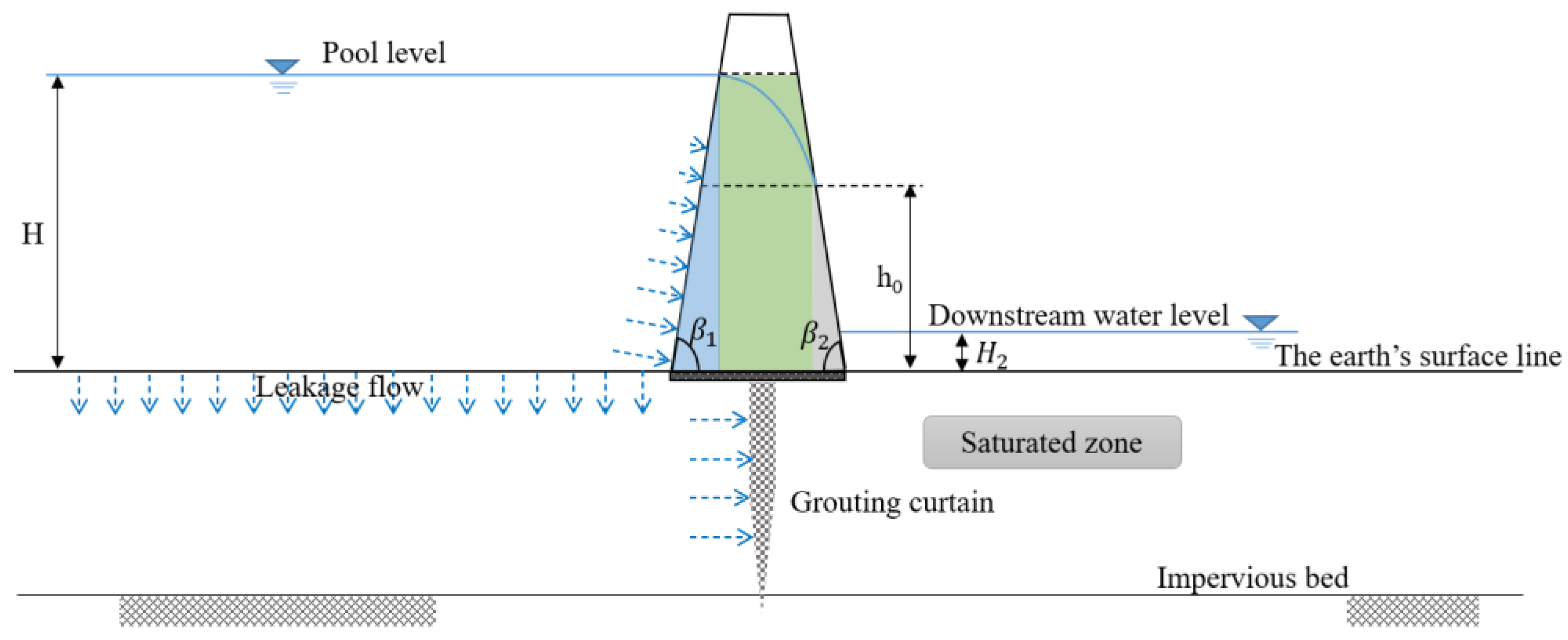
Figure 1 is the cross-section of a simplified clay core dam. Some basic assumptions can be made for the calculation of seepage:
(1) The position of the groundwater level remains constant.
The focus of the following analytical method is to estimate the leakage amount in a steady state, and an unchanged groundwater level is necessary.
(2) There is no centralized leakage channel in the reservoir area or dam body.
It is a common engineering problem that there exists a centralized leakage channel, through which a large amount of leakage water may flow away. The focus of this problem is how to find the leakage channel and plug it effectively, rather than calculate the seepage flow of the centralized leakage channel. Therefore, the centralized leakage channel is not considered in this paper.
(3) The rock-soil body is homogeneous and isotropic.
In practical engineering, the geological conditions and project design are more complex and detailed. The rock-soil body is often inhomogeneous and anisotropic, and it is difficult to homogenize the dam filling. For example, some dam site areas are layered with inclination of layers, and probably result in anisotropy. It is unrealistic and complex to obtain the analytical solutions considering the geological conditions in detail. Therefore, such an assumption is needed in practical engineering to gain hydraulic conductivities of different zones for leakage estimation.
(4) Rock, soil, and water are incompressible, and the pore size and porosity of soil mass remain unchanged.
(5) The lag of the soil moisture characteristic curve and its correlation with volume deformation should be ignored.
Studies on the seepage of earths dam usually focus on the gravitational water, which is a very complex problem, and it needs to be simplified in the analytical calculation. The structure of rock-soil body, the shape and size of particles, the porosity, and the saturation of water all affect the permeability. Therefore, in order to facilitate the calculation, assumptions (3)–(5) need to be made. Many engineering examples show that the calculation results can meet the accuracy requirements of the project if they are assumed to be within the allowable range. In the seepage field, if only a local area does not meet the assumptions of (3)–(5), the results are still reliable [43].
2.2. Simplified Calculation Method
According to different groundwater levels, i.e., below or above the reservoir bottom, the simplified calculation can be mainly divided into two situations.
2.2.1. Groundwater Level below the Reservoir Bottom
(1) The groundwater level is deep.
When the groundwater level is deep, the rock-soil body below the reservoir is unsaturated. Since the hydraulic conductivity of the rockfill area is much greater than that of the core, the role of the rockfill area in dam anti-seepage is usually ignored. The leakage amount of the clay core dam is mainly associated with the hydraulic conductivity of the core and the reservoir bottom.
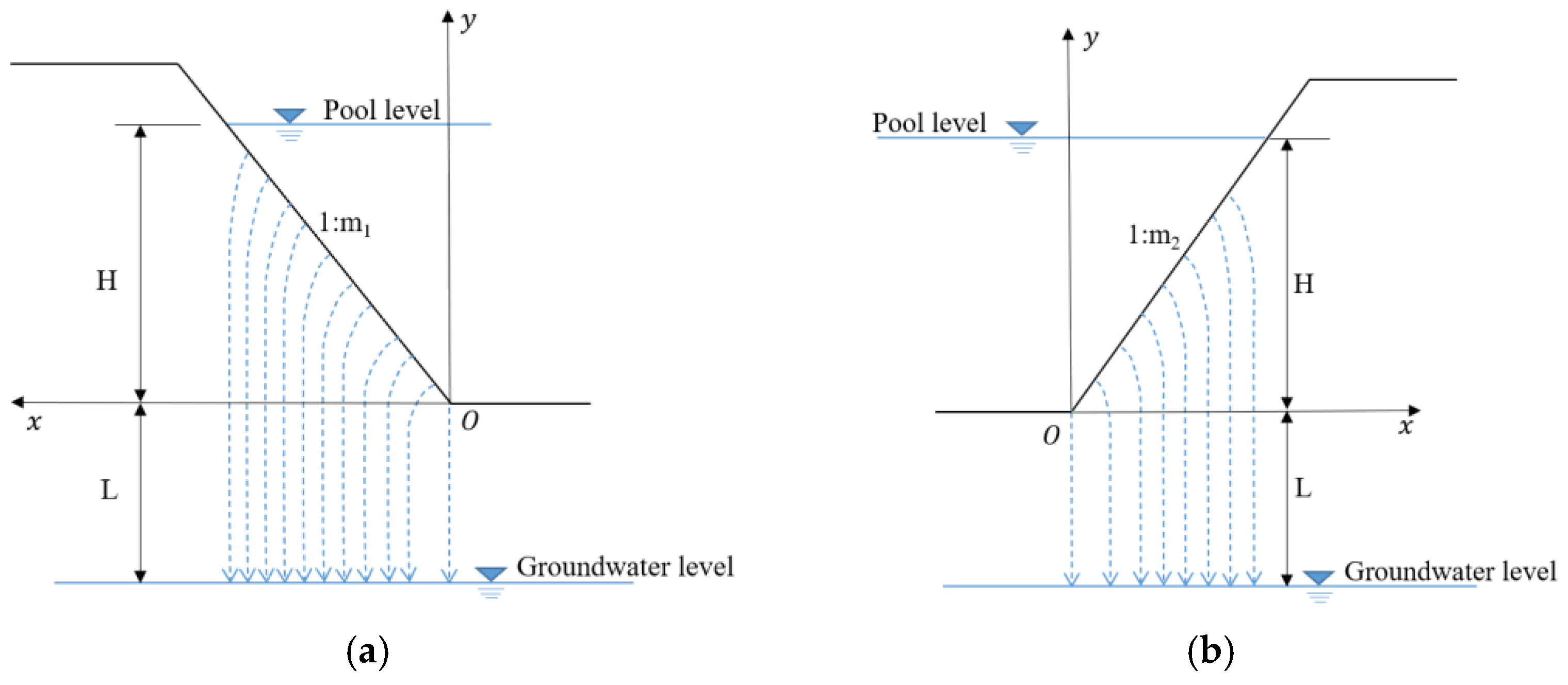
For leakage from the reservoir bottom, there are two main periods after the reservoir starts filling. Firstly, the leakage water from the reservoir gradually wets the rock-soil body to the groundwater level. With the increase in the range of the wet rock-soil body, the leakage amount will decrease gradually. This period can be called the unsteady free leakage stage (Figure 2a). Secondly, the leakage amount will remain constant. There is no direct hydraulic association between the leakage water and the groundwater; as a result, the leakage amount will not change. This period can be called the steady free leakage stage (Figure 2b).
In the steady leakage stage, the leakage amount relates to the size of the reservoir and the hydraulic conductivity of the rock-soil body below the reservoir. In Figure 2, the slopes on both sides of the reservoir are 1:m1 and 1:m2. The seepage flux can be calculated as follows [43]:
where represents the seepage flux per unit length of reservoir, m2/s; represents the hydraulic conductivity of the rock-soil body close to the reservoir, m/s; represents the width of the pool level in the cross-section of the reservoir, m; is height of the pool level, m; and is the coefficient depending on the value of , , and . The value of can be determined empirically by Figure 3 [43].
The total leakage from the reservoir bottom can be written as follows:
where is the length upstream of the dam body, m. If the shape of the reservoir valley section substantially varies, data from multiple sections should be taken for averaging to obtain the total leakage from the reservoir bottom.
For leakage from the core, the core can be divided into three sections, i.e., the upstream section (blue section), the middle section (green section), and the downstream section (gray section), as is shown in Figure 4. is the angle of the upstream slope of the core, and is the angle of the downstream slope of the core. is the height of the seepage face at the intersection of the phreatic line and downstream slope.
In the upstream section, the triangular region can be transformed into an equivalent rectangular region for the convenience of seepage flux calculation. As is shown in Figure 5, a rectangular coordinate system can be established.
The basic assumption of Dupuit’s equation is that the pressure at each point on the section conforms to the hydrostatic pressure distribution—that is, the piezometric heads along the vertical are equal, and the isohead line is a vertical line. This situation is only approximate when the seepage flow is slowly changing. Many experimental studies show that the seepage movement in the middle section of the earth dam is a slowly changing seepage movement, so the application of Dupuit’s equation is also approximate [43]. According to the analysis of Dupuit’s equation and relevant test data, Dupuit’s equation has sufficient accuracy.
The width of the equivalent rectangular region depends on the seepage resistance of the upstream section, which is associated with the values of and . According to the solution of fluid mechanics, a semi-empirical formula can be presented:
where denotes the width of the equivalent rectangular region, m. According to Dupuit´s postulates, the seepage flux per unit through the upstream section and the middle section can be written as [43]:
where is the pool level, m; is the bottom width of the middle section and the downstream section, m; and is the hydraulic conductivity of the core, m/s. The discharge per unit through the downstream section can be written as:
According to the continuity equation, the seepage flux through different sections should remain constant. Hence, the value of is equal to . Combining Equations (4) and (5), the following equation can be obtained as:
The solution of the above equation is:
When , the value of is greater than the pool level , which is unreasonable. As a result, the value of should be .
Therefore, we substitute the value of into Equation (5), and the seepage flux per unit through the core can be obtained as:
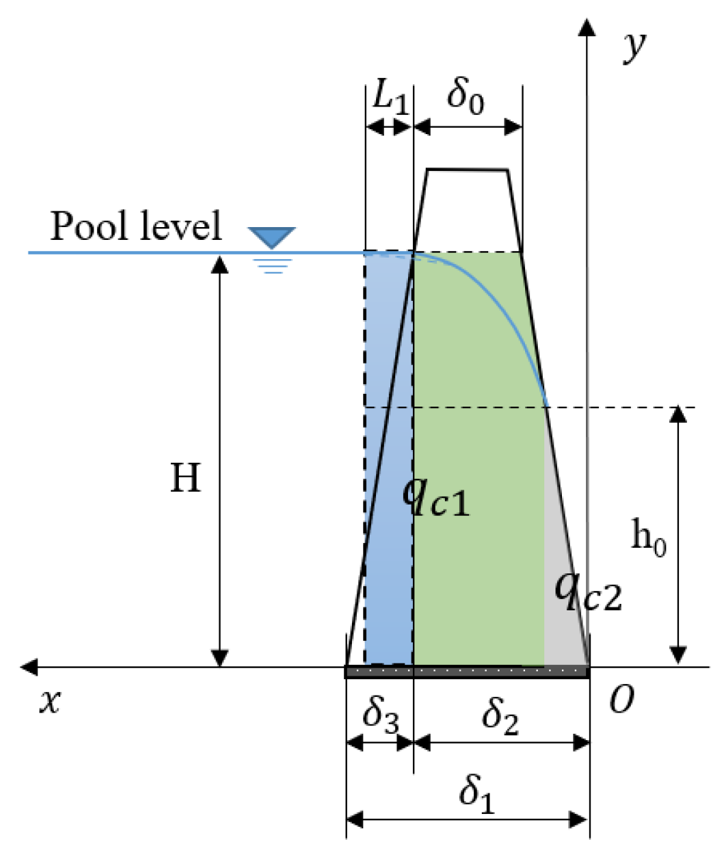
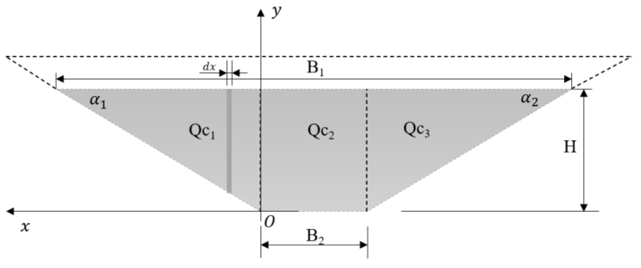
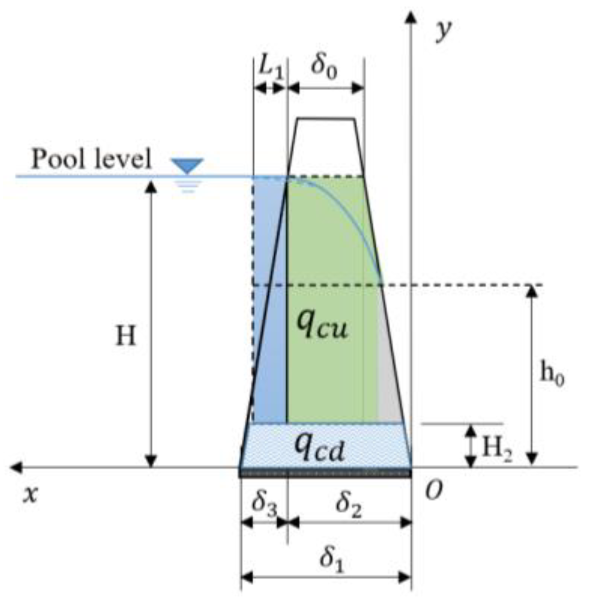
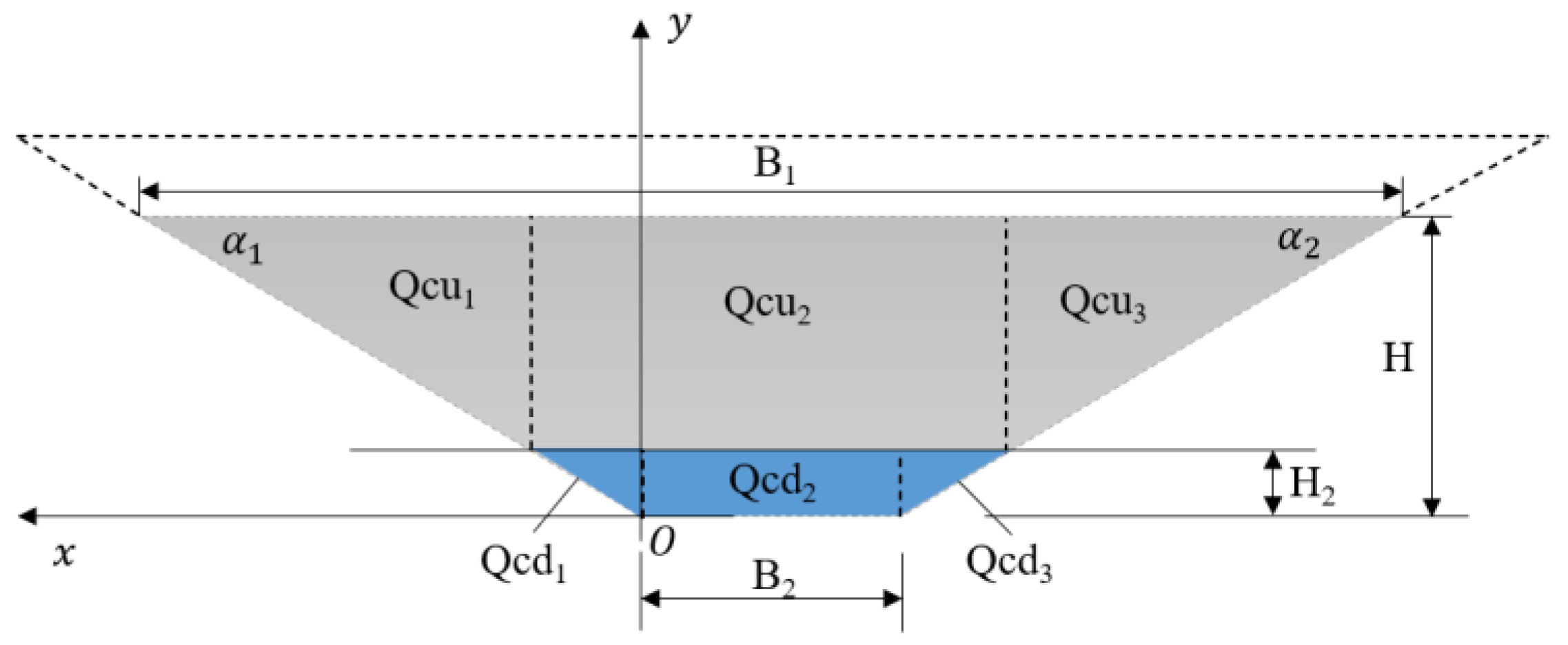
The longitudinal section of the core can be simplified as a trapezoid, as is shown in Figure 6. The gray part of the longitudinal section is below the pool level. and represent the length, m, of the top and bottom of the gray part, respectively. and represent the included angle between the left and right sides of the core and the horizontal plane, respectively. The core can be divided into three parts for convenience of calculation.
The seepage flux through the middle rectangular part can be written as:
To calculate the discharge through the left part , a rectangular coordinate system, as shown in Figure 6, can be established.
Considering the seepage flux over the length , the seepage flux can be written as:
Integrating Equation (10) with from 0 to , the seepage flux can be obtained as:
where .
Similarly, the seepage flux through the right part can be written as:
The total leakage from the core can be written as:
The total leakage of the clay core dam is combined by two parts, i.e., leakage from the reservoir bottom and leakage from the core, and it can be written as follows:
(2) The groundwater level is shallow.
In this situation, leakage from the reservoir bottom continuously replenishes groundwater, and the area below the reservoir bottom is saturated. There exists hydraulic association between the leakage water and the groundwater; as a result, the leakage amount relates not only to the permeability of the rock-soil body below the reservoir, but also to the position of the groundwater level. As is shown in Figure 7, leakage water flows into the rock-soil body vertically, and then flows towards the groundwater.
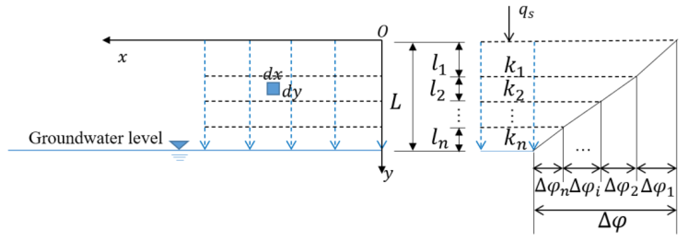
For leakage from the reservoir bottom, a rectangular system, as shown in Figure 8, can be established. Suppose that the rock-soil body below the reservoir has layers. and are the thickness and the hydraulic conductivity of each layer, respectively. is the hydraulic head drop of each layer.
Based on Darcy’s law, the discharge through the reservoir can be written as [31]:
where represents the reservoir bottom length, m, in the cross-section.
Therefore, can be written as:
It should be noted that .
Then, the total drop can be written as [35]:
Replacing the above formation system with a continuous variation of hydraulic permeability, Equation (17) can be written as:
By integrating Equation (18), the head drop at depth can be written as:
As a result, if the hydraulic head drop is known, the seepage flux can be easily obtained as follows:
The leakage from the bottom of the reservoir can be written as:
For leakage from the reservoir periphery, rectangular systems, as shown in Figure 9, can be established.
According to Equation (20), the seepage flux through the periphery of the reservoir on the left side (shown in Figure 9a) can be obtained as follows:
Similarly, the seepage flux through the periphery of the reservoir on the right side (shown in Figure 9b) can be obtained as follows:
The total leakage from the reservoir bottom can be written as:
For leakage from the core, because the downstream water level is still below the reservoir bottom, the calculation of the seepage flux can refer to Equations (9), (11), and (12).
The total leakage from the core can be written as:
The total leakage of the clay core dam can be expressed as follows:
(3) The above two situations can be distinguished according to the following standards.
Assuming that the water table is far from the earth surface, the seepage flux from the reservoir bottom can be written as follows, according to Equation (2):
Additionally, according to Equations (21)–(24), the seepage flux from the reservoir bottom can be written as follows:
Combining Equations (27) and (28), the value of can be obtained.
Therefore, when , Equation (2) can be applied, and when , Equation (24) can be applied.
2.2.2. Groundwater Level above the Reservoir Bottom
In this case, the rock-soil body below the groundwater level is saturated and the downstream water level is higher than the reservoir bottom. There exists hydraulic association between the reservoir leakage and the groundwater. The calculation of the seepage flux mainly considers the hydraulic conductivity of the rock-soil body and the core, as well as the position of the downstream water level.
For leakage from the reservoir bottom, Figure 10 is the cross-section of the reservoir for simplified calculation.
Referring to Equation (21), the seepage flux through the reservoir bottom can be obtained as:
where represents the depth of the saturated zone, m, and represents the distance between the groundwater level and the reservoir bottom, m.
Similar to situation in which the groundwater level is close to reservoir bottom, as is shown in Figure 11, the seepage flux through both sides of the periphery of the reservoir (Figure 11a), (Figure 11b) can be obtained as:
Therefore, the total leakage from the reservoir can be written as:
For leakage from the core, like the previous segmentation method, the simplified diagram of the calculation is shown in Figure 12. is the downstream water level.
To calculate the seepage flux through the core, the core can be divided into two parts to calculate the seepage flow separately, i.e., the part of core below the downstream water level and the part of core above the downstream water level, as is shown in Figure 13.
In the part of core below the downstream water level, the seepage flux can be calculated as seepage under pressure. To calculate the seepage flux through this part, a rectangular coordinate system, as shown in Figure 13, can be established. Based on Darcy’s law, the discharge through this part can be written as:
By integrating Equation (33) with from 0 to , the seepage flux through this part can be obtained as follows:
In the part of core above the downstream water level, the calculation of seepage flux is similar to Equation (8), which can be written as:
In Equation (35), and respectively represent:
The longitudinal section of the core can be simplified as a trapezoid, as is shown in Figure 14. The gray part of the longitudinal section is between the upstream water level and the downstream water level, and the blue part is below the downstream level. The core can be divided into six parts for convenience of calculation.
The seepage flux through the middle rectangular blue part can be written as:
To calculate the seepage flux through the left blue part , a rectangular coordinate system, as shown in Figure 14, can be established.
Considering the seepage flux over the length , the seepage flux can be written as:
Integrating Equation (39) with from 0 to , the seepage flux can be obtained as:
where .
Similarly, the seepage flux through the right part can be written as:
To calculate the seepage flux through the gray part, the solutions to , , and , referring to Equations (9), (11), and (12), can be obtained as follows:
where and .
The total leakage from the core can be written as:
The total leakage of the clay core dam can be expressed as follows:
2.3. Case Verification
To prove the rationality of the proposed formulae, a simple numerical model of a clay core dam was established using Geo-studio 2020 SEEP/W [49], as is shown in Figure 15. Figure 15a is the cross-section of the core. The width of the bottom of the core is 40 m, the angle of the upstream slope of the core is 77.5°, and the angle of the downstream slope of the core is 78.1°. The hydraulic conductivity of the core is 1 × 10⁻⁹ m/s. Figure 15b is the cross-section of the reservoir. The width of the bottom of the reservoir is 59 m, the slope on the left side of the reservoir is 1:1.3, and the slope on the right side of the reservoir is 1:1.2. The rock-soil body can be divided into four layers under the reservoir, and the thicknesses and hydraulic conductivities are listed in Table 1.
For leakage from the reservoir bottom, suppose the pool level is 50 m; when the groundwater level is below the reservoir bottom, the value of can be solved as 11.36 m. As a result, when = 5 m, Equation (24) should be used, and when = 40 m, Equation (2) should be used. When the groundwater level is above the reservoir bottom, Equation (32) should be used.
For leakage from the core, suppose the pool level is 50 m; when the downstream water level is below the reservoir bottom, Equation (13) should be used; when the downstream water level is above the reservoir bottom, Equation (45) should be used. By applying the proposed analytical method and the Geo-studio 2020 SEEP/W analysis, the seepage flux can be calculated.
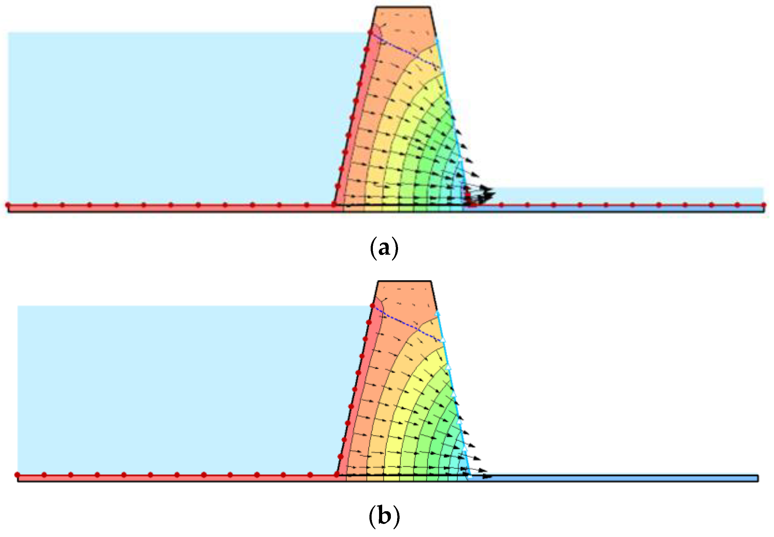
The calculation results are shown in Table 2 and Table 3. Figure 16 and Figure 17 are the streamline directions analyzed by Geo-studio 2020, and different areas in different colors represent different equipotential regions.
Based on the above results, the analytical results are consistent with the software modeling results in calculating the discharge of both the reservoir bottom and the core, where the relative errors are less than 10%. By this simple case, it is verified that the proposed method is reliable.
3. Engineering Application
The Jinsha River is the name for the upper reaches of the Yangtze River. It originates from the southern foot of the Bayankala Mountains in Yushu County, Qinghai Province. Its largest tributary is the Yalong River. The total length of the river is about 1570 km, and the drainage area is about 136,000 km2, accounting for about 27.1% of the catchment area of the Jinsha River (above Yibin). The average annual discharge of the estuary is 1930 m3/s, and the annual runoff is 60.9 billion m3. The Lianghekou hydropower station is located on the main stream of the Yalong River in Yajiang Country, Sichuan Province, China (shown in Figure 18).
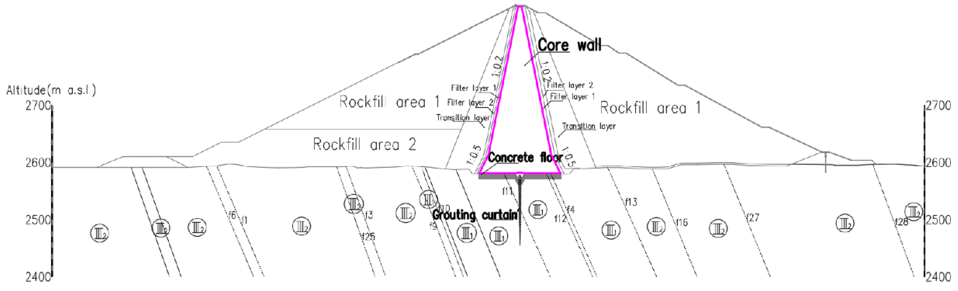
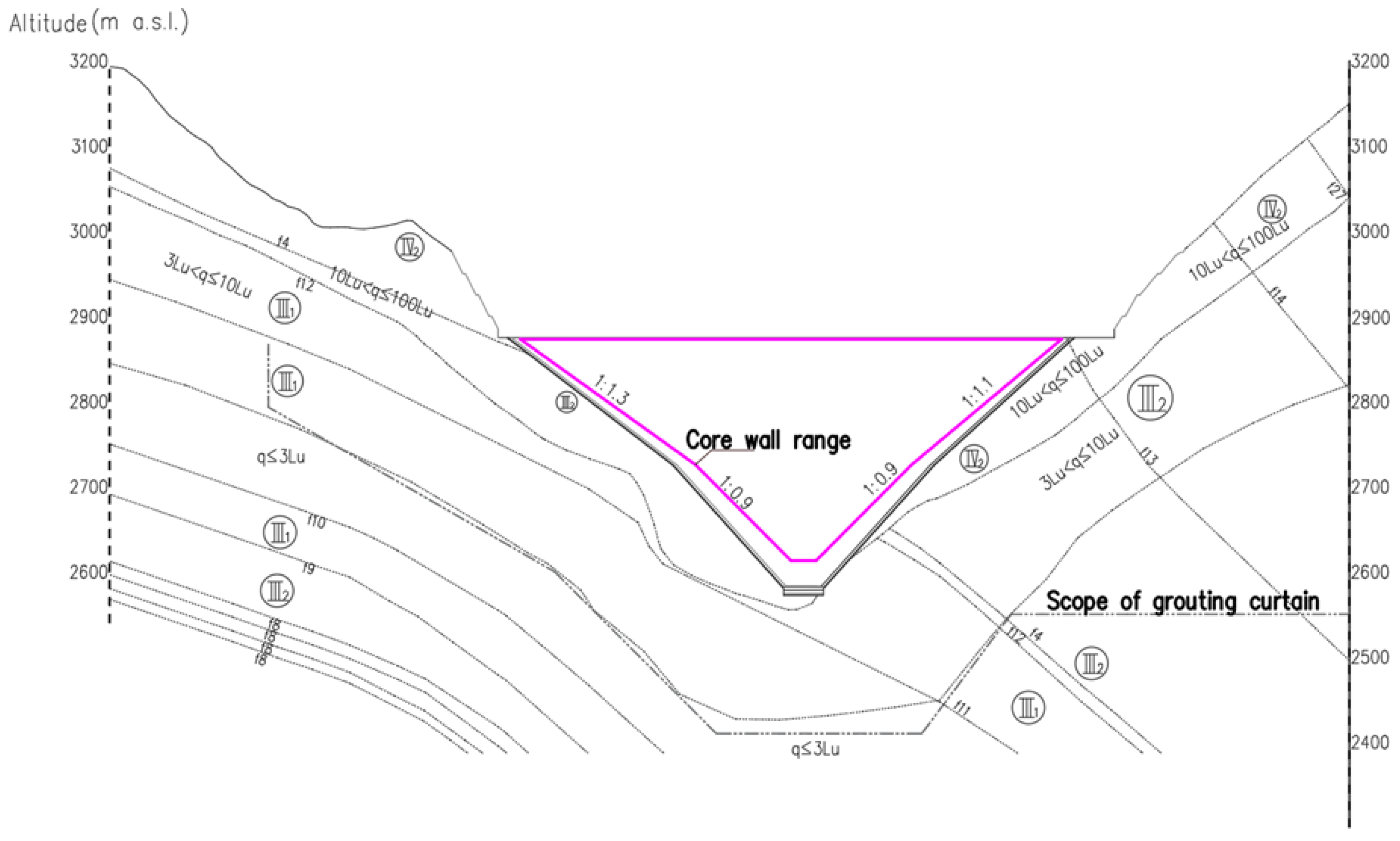
The power station adopts a clay core dam to store water and generate electricity, with a maximum dam height of 295 meters. The normal pool level of the reservoir is 2865.00 m a.s.l., and the storage is more than 10 billion m3. The dam crest elevation is 2875.00 m a.s.l., and the excavation elevation of the core bottom is 2580.00 m a.s.l. The top width of the core is 6 m, the top elevation is 2874.00 m a.s.l., and the upstream and downstream slope ratio of the core are both 1:0.2. The bottom width of the core is 153 m and the bottom elevation is 2583.00 m a.s.l. The cross-sections of the dam body and the reservoir are shown in Figure 19 and Figure 20, and the region in magenta is the range of the core. In Figure 19 and Figure 20, different areas of the dam body have been marked. Circled Roman numerals indicate different rock grades and “f+ numerals” indicate different faults.
Based on the occurrence conditions of groundwater and the characteristics of water-bearing medium, lithology, and its combination, the types of groundwater are divided into loose accumulation layer pore phreatic water and bedrock fissure water. The bedrock fissure water is shallow weathering unloading bedrock fissure water and fissure-confined water. The spatial form of groundwater in the dam site area is pore phreatic water and bedrock fissure water, and the lower part is fissure-confined water. Pore phreatic water is related to the distribution of overburden and is locally exposed. Shallow weathering unloading fissure water is exposed in the weathering unloading zone of rock mass. The phreatic water is generally a one-sided aquifer with a relatively stable groundwater level. Fissure-confined water is mainly exposed in siltstone and fine sandstone, which is a banded water-bearing body. The river valley in the dam area is deep and the bank slope is steep. Generally, the groundwater supplies the river water. Based on engineering geological and hydrogeological data, the hydraulic conductivities of different zones of the dam body are shown in Table 4, and the hydraulic conductivities of different layers of the rock-soil body under the reservoir bottom are shown in Table 5.
3.1. Analytical Solution
The normal pool level is 2865.00 m a.s.l., and the downstream water level is 2610 m a.s.l., indicating that Equations (32) and (45) should be used to calculate the seepage flux of the reservoir and the dam body, respectively. The values of different parameters in this condition are listed in Table 6.
3.2. Numerical Solution
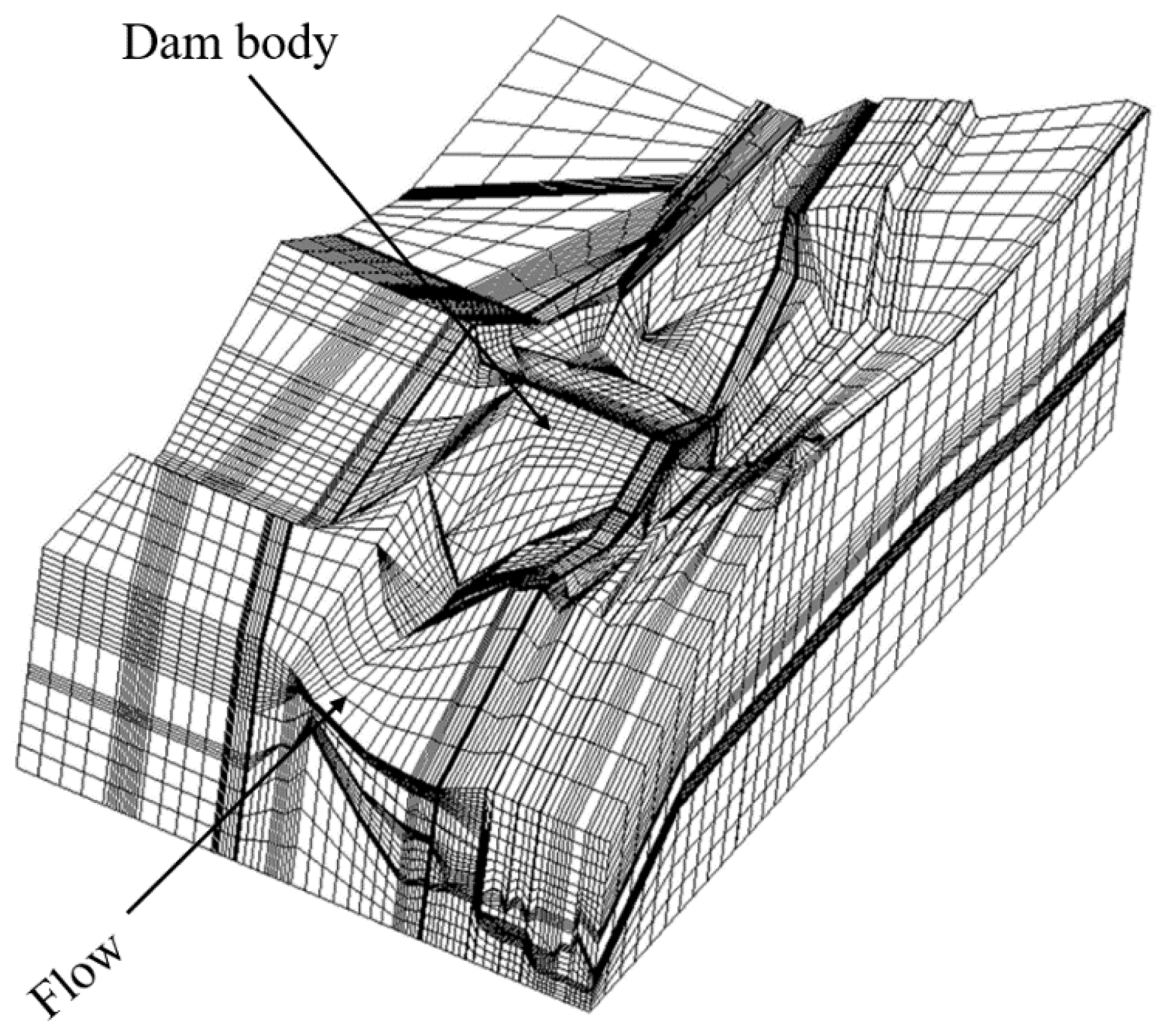
In addition to the proposed analytical method, an FEM numerical method was built to model the seepage field of the clay core dam. Figure 21 is the three-dimensional model of the reservoir area. The numerical calculation adopts the self-developed three-dimensional stable seepage finite element calculation and analysis program, whose reliability has been proven in the seepage calculation of dozens of water conservancy projects at home and abroad. The zone below the water level of the upstream reservoir and the location of the groundwater level have a Dirichlet boundary. The bottom and surroundings of the model are considered as an aquifuge, with a Neumann boundary. The top of the model is a free surface boundary. Other calculation parameters are the same as in Section 3.1.
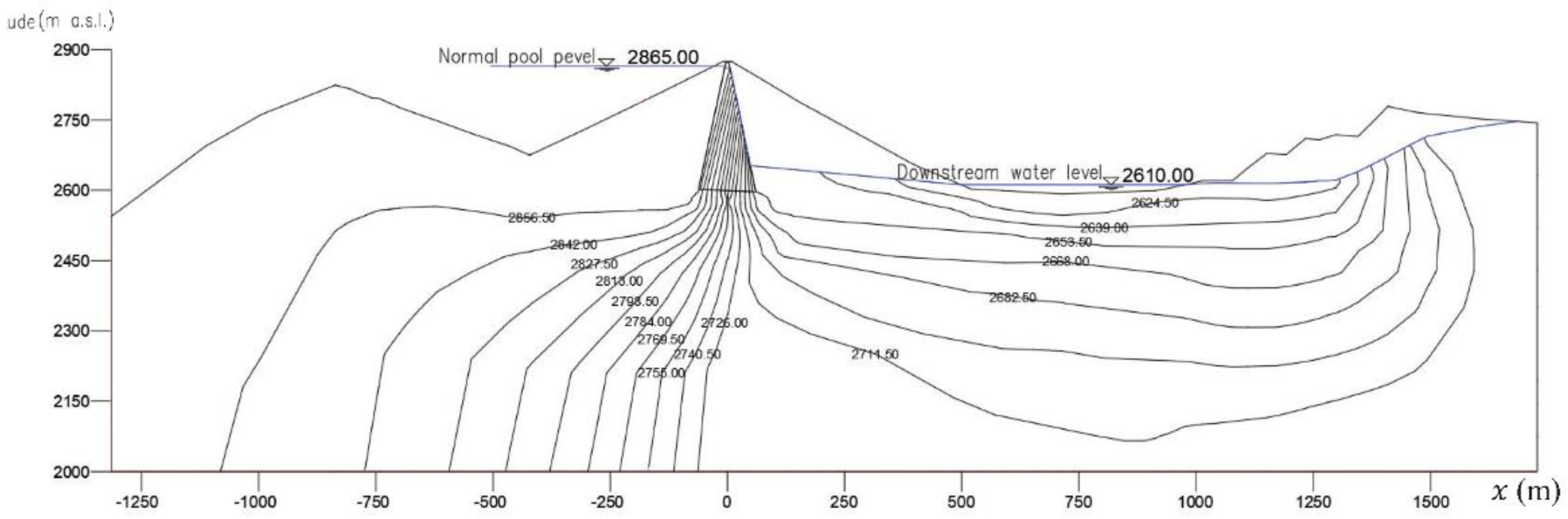
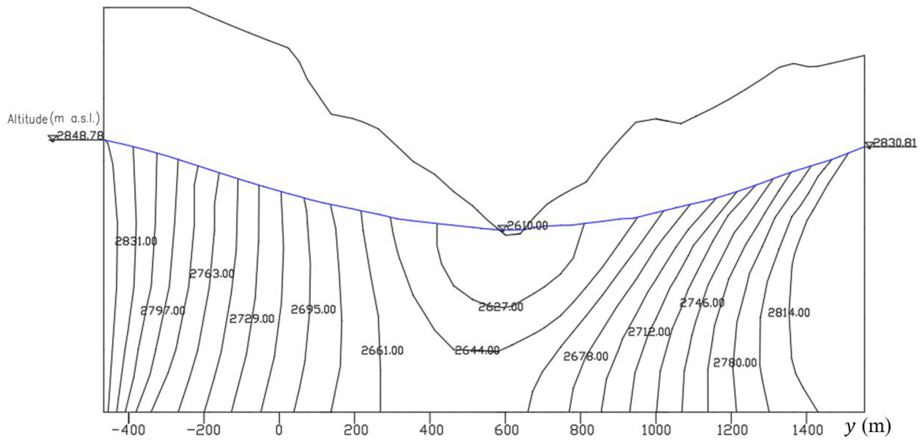
The potential distribution of the cross-section of the dam body is shown in Figure 22, and the potential distribution of the cross-section of the reservoir is shown in Figure 23.
The calculation results of both numerical and analytical methods for the leakage of the clay core dam are presented in Table 7.
The results gained by the analytical method are consistent with those obtained by the numerical method, where the relative errors are less than 10%, indicating that the simplified method is feasible in engineering applications. The leakage amount from the core is far less than that from the reservoir bottom with the condition of a normal pool level, which reflects the good anti-seepage performance of the core. To reduce the leakage amount in case of a determined hydrogeological condition, more targeted engineering measures should be taken to control the seepage flux of the reservoir bottom, such as laying face slab for retaining water, geomembranes, etc.
4. Conclusions
To obtain the leakage amount of the clay core dam in a short time, we proposed a simplified analytical method. The proposed method is composed of two sets of formulae according to different conditions of the position of the groundwater level, i.e., below or above the reservoir bottom. Both formulae can be used to calculate the seepage flux of the dam body and the reservoir bottom, which are the main leakage zones of a clay core dam. To prove the rationality of the proposed method, a numerical model was built using Geo-studio 2020 SEEP/W to calculate the discharge of the clay core dam, where the relative errors between the results are no more than 10%, indicating the rationality of the analytical method. In leakage estimation of the clay core dam of the Lianghekou power station, the results obtained by the proposed analytical method and the numerical method are close, and the relative errors are no more than 10%, showing the feasibility of the proposed method in engineering applications.
In engineering applications, the proposed method can help obtain the leakage amount and evaluate the rationality of the clay core dam quickly in the design state without the tedious and time-consuming modeling process of numerical methods. It is of vital importance to estimate the leakage amount of clay core dams before the engineering is commenced, which not only relates to the safe operation of the project, but is also related to the economic benefits of the project. The proposed analytical method can offer a solution for leakage amount estimation by striking a balance between precision and efficiency.
Author Contributions
Conceptualization, C.Y. and Z.S.; methodology, C.Y.; software, C.Y. and L.X.; validation, C.Y. and H.S.; writing—original draft preparation, C.Y.; writing—review and editing, L.X. All authors have read and agreed to the published version of the manuscript.
Funding
This research was funded by the National Key R&D Program of China (grant number 2019YFC1510802) and National Natural Science Foundation of China (grant number 52179130).
Institutional Review Board Statement
Not applicable.
Conflicts of Interest
The authors declare no conflict of interest.
Abbreviations
| Variables | Meanings |
| Height of the pool level | |
| Distance between the groundwater level and the earth surface line | |
| Downstream water level | |
| Length of the reservoir bottom in the cross-section | |
| Length of the top of the longitudinal section of the core | |
| Length of the bottom of the longitudinal section of the core | |
| Geometric parameter of core dimension, shown in Figure 5 | |
| Geometric parameter of core dimension, shown in Figure 5 | |
| Geometric parameter of core dimension, shown in Figure 5 | |
| Geometric parameter of core dimension, shown in Figure 5 | |
| Length upstream of the dam body | |
| Angle of the upstream slope of the core | |
| Angle of the downstream slope of the core | |
| Angle parameter, shown in Figure 6 | |
| Angle parameter, shown in Figure 6 | |
| Hydraulic conductivity of the core | |
| Hydraulic conductivities of different layers of the rock-soil body |
References
- Díaz-González, F.; Sumper, A.; Gomis-Bellmunt, O.; Villafáfila-Robles, R. A review of energy storage technologies for wind power applications. Renew. Sustain. Energy Rev. 2012, 16, 2154–2171. [Google Scholar] [CrossRef]
- Alonso, E.E.; Olivella, S.; Pinyol, N.M. A review of Beliche Dam. Géotechnique 2005, 55, 267–285. [Google Scholar] [CrossRef]
- Berhane, G.; Martens, K.; Al Farrah, N.; Walraevens, K. Water leakage investigation of micro-dam reservoirs in Mesozoic sedimentary sequences in northern Ethiopia. J. Afr. Earth Sci. (1994) 2013, 79, 98–110. [Google Scholar] [CrossRef]
- Chen, Y.; Hong, J.; Zheng, H.; Li, Y.; Hu, R.; Zhou, C. Evaluation of Groundwater Leakage into a Drainage Tunnel in Jinping-I Arch Dam Foundation in Southwestern China: A Case Study. Rock Mech. Rock Eng. 2016, 49, 961–979. [Google Scholar] [CrossRef]
- Mozafari, M.; Milanović, P.; Jamei, J. Water leakage problems at the Tangab Dam Reservoir (SW Iran), case study of the complexities of dams on karst. Bull. Eng. Geol. Environ. 2021, 80, 7989–8007. [Google Scholar] [CrossRef]
- Abedian, H.; Karami, G.H.; Karimi, H. The effect of scale on the water leakage from the reservoir and abutment of Beheshtabad Dam. Bull. Eng. Geol. Environ. 2019, 78, 5569–5581. [Google Scholar] [CrossRef]
- Adinehvand, R.; Raeisi, E.; Hartmann, A. An integrated hydrogeological approach to evaluate the leakage potential from a complex and fractured karst aquifer, example of Abolabbas Dam (Iran). Environ. Earth Sci. 2020, 79, 1–19. [Google Scholar] [CrossRef]
- Zhong, Q.; Wang, L.; Chen, S.; Chen, Z.; Shan, Y.; Zhang, Q.; Ren, Q.; Mei, S.; Jiang, J.; Hu, L.; et al. Breaches of embankment and landslide dams—State of the art review. Earth-Sci. Rev. 2021, 216, 103597. [Google Scholar] [CrossRef]
- Říha, J.; Švancara, J. The Failure of the Mostiště Embankment Dam; Thomas Telford Publishing: Durham, UK, 2006. [Google Scholar]
- Mattsson, H.; Hellström, J.G.I.; Lundström, T.S. On Internal Erosion in Embankment Dams: A Literature Survey of the Phenomenon and the Prospect to Model It Numerically; Luleå University of Technology, Department of Civil, Mining and Environmental Engineering, Division of Mining and Geotechnical Engineering: Luleå, Sweden, 2008. [Google Scholar]
- Sam, J. Seepage Monitoring in Embankment Dams; Kungliga Tekniska Hogskolan: Stockholm, Sweden, 1997. [Google Scholar]
- Cheng, L.; Zhang, A.; Cao, B.; Yang, J.; Hu, L.; Li, Y. An experimental study on monitoring the phreatic line of an embankment dam based on temperature detection by OFDR. Opt. Fiber Technol. 2021, 63, 102510. [Google Scholar] [CrossRef]
- Sjödahl, P.; Dahlin, T.; Johansson, S.; Loke, M.H. Resistivity monitoring for leakage and internal erosion detection at Hällby embankment dam. J. Appl. Geophys. 2008, 65, 155–164. [Google Scholar] [CrossRef] [Green Version]
- Ghafoori, Y.; Vidmar, A.; Říha, J.; Kryžanowski, A. A Review of Measurement Calibration and Interpretation for Seepage Monitoring by Optical Fiber Distributed Temperature Sensors. Sensors 2020, 20, 5696. [Google Scholar] [CrossRef]
- Bathe, K.J.; Khoshgoftaar, M.R. Finite element free surface seepage analysis without mesh iteration. Int. J. Numer. Anal. Met. 1979, 3, 13–22. [Google Scholar] [CrossRef] [Green Version]
- Aldulaimi, A.A. Safety evaluation of the chamrga earth dam. a seepage deformation, and stability analysis with GeoStudio. IOP Conf. Series. Earth Environ. Sci. 2021, 664, 12075. [Google Scholar] [CrossRef]
- Salmasi, F.; Norouzi, R.; Abraham, J.; Nourani, B.; Samadi, S. Effect of Inclined Clay Core on Embankment Dam Seepage and Stability through LEM and FEM. Geotech. Geol. Eng. 2020, 38, 6571–6586. [Google Scholar] [CrossRef]
- Li, H.; Zhao, F.; Li, J. Seepage analysis of clay core wall dam based on ABAQUS. IOP Conf. Ser. Earth Environ. Sci. 2019, 384, 12015. [Google Scholar] [CrossRef]
- Elkamhawy, E.; Zelenakova, M.; Abd-Elaty, I. Numerical Canal Seepage Loss Evaluation for Different Lining and Crack Techniques in Arid and Semi-Arid Regions: A Case Study of the River Nile, Egypt. Water 2021, 13, 3135. [Google Scholar] [CrossRef]
- Fukuchi, T. Numerical analyses of steady-state seepage problems using the interpolation finite difference method. Soils Found. 2016, 56, 608–626. [Google Scholar] [CrossRef]
- Hansen, D.; Roshanfekr, A. Assessment of Potential for Seepage-Induced Unraveling Failure of Flow-through Rockfill Dams. Int. J. Geomech. 2012, 12, 560–573. [Google Scholar] [CrossRef]
- Lee, S.S. Finite-Difference Method Three-Dimensional Model for Seepage Analysis through Fordyce DAM. In Advances in Geosciences; World Scientific: Singapore, 2007; Volume 6, pp. 171–180. [Google Scholar]
- Chang, C.S. Boundary element method in drawdown seepage analysis for earth dams. J. Comput. Civ. Eng. 1987, 1, 83–98. [Google Scholar] [CrossRef]
- Sánchez-Sesma, F.J.; Arellano-Guzmán, M.; Pérez-Gavilán, J.J.; Suarez, M.; Marengo-Mogollón, H.; Chaillat, S.; Jaramillo, J.D.; Gómez, J.; Iturrarán-Viveros, U.; Rodríguez-Castellanos, A. Seismic response of three-dimensional rockfill dams using the Indirect Boundary Element Method. IOP Conf. Ser. Mater. Sci. Eng. 2010, 10, 12167. [Google Scholar] [CrossRef]
- Seeda, A.; Mohamed, H. Nonlinear Seismic Response of Dams Using a Coupled Boundary Element—Finite Element Formulation; Rice University: Houston, TX, USA, 1996. [Google Scholar]
- Chen, K.; Zou, D.; Kong, X.; Chan, A.; Hu, Z. A novel nonlinear solution for the polygon scaled boundary finite element method and its application to geotechnical structures. Comput. Geotech. 2017, 82, 201–210. [Google Scholar] [CrossRef]
- Smith, N.S.; Ravindra, G.H.R.; Sigtryggsdóttir, F.G. Numerical Modeling of the Effects of Toe Configuration on Throughflow in Rockfill Dams. Water 2021, 13, 1726. [Google Scholar] [CrossRef]
- Beiranvand, B.; Komasi, M. An Investigation on performance of the cut off wall and numerical analysis of seepage and pore water pressure of Eyvashan earth dam. Iran. J. Sci. Technol. Trans. Civ. Eng. 2021, 45, 1723–1736. [Google Scholar] [CrossRef]
- Nourani, V.; Behfar, N.; Dabrowska, D.; Zhang, Y. The Applications of Soft Computing Methods for Seepage Modeling: A Review. Water 2021, 13, 3384. [Google Scholar] [CrossRef]
- Parsaie, A.; Haghiabi, A.H.; Latif, S.D.; Tripathi, R.P. Predictive modelling of piezometric head and seepage discharge in earth dam using soft computational models. Environ. Sci. Pollut. Res. 2021, 28, 60842–60856. [Google Scholar] [CrossRef]
- Bear, J. Dynamics of Fluids in Porous Media; American Elsevier Publishing Company, Inc.: Amsterdam, The Netherlands, 1972. [Google Scholar]
- Bear, J.; Verruijt, A. Modeling Groundwater Flow and Pollution; D.Reidel Publishing Company: Dordrecht, The Netherlands, 1992. [Google Scholar]
- Říha, J. Groundwater Flow Problems and Their Modelling. In Assessment and Protection of Water Resources in the Czech Republic; Zelenakova, M., Fialová, J., Negm, A.M., Eds.; Springer International Publishing: Cham, Switzerland, 2020; pp. 175–199. [Google Scholar]
- Charny, I.A. Calculation of the Lowering of the Free Surface in a Dam for Changed Level of the Downstream Level; Academy of Science: Moscow, Russia, 1953. [Google Scholar]
- Girinski, N.K. Calculation of Seepage under Hydraulic Structures in Non-Homogeneous Soils; Gostrojizdat: Moscow, Russia, 1941. [Google Scholar]
- Pavlovsky, N.N. On Seepage of Water Through Earth Dams; Kubuch: Leningrad, Russia, 1931. [Google Scholar]
- Dachler, R. Grundwasserstromung; Springer: Wien, Austria, 1936. [Google Scholar]
- Davison, B.; Rosenhead, L. Some cases of the steady two-dimensional percolation of water through ground. Proc. R. Soc. Lond. Ser. A Math. Phys. Sci. 1940, 175, 345–365. [Google Scholar]
- Casagrande, A. Seepage through dams. In Contributions to Soil Mechanics 1925–1940; Boston Society of Civil Engineers: Boston, MA, USA, 1940; pp. 295–336. [Google Scholar]
- Nelson-Skornyakov, F.B. Seepage in Homogeneous Media; Sovetskaya Nauka: Moscow, Russia, 1949. [Google Scholar]
- Aravin, V.I.; Numerov, S.N. Theory of Fluid Flow in Undeformable Porous Media; Gostekhizdat: Moscow, Russia, 1953. [Google Scholar]
- Aravin, V.N.; Numerov, S.N. Calculation of Seepage in Hydraulic Structures; GILSA: Leningrad, Russia, 1955. [Google Scholar]
- Mao, C. Seepage Computation Analysis & Control, 2nd ed.; China Water & Power Press: Beijing, China, 2003; pp. 255–256. [Google Scholar]
- Kacimov, A.R.; Al-Maktoumi, A.; Obnosov, Y.V. Seepage through earth dam with clay core and toe drain: The Casagrande-Numerov analytical legacy revisited. ISH J. Hydraul. Eng. 2021, 27, 264–272. [Google Scholar] [CrossRef]
- Kacimov, A.; Obnosov, Y. Analytical solutions for seepage near material boundaries in dam cores: The Davison–Kalinin problems revisited. Appl. Math. Model. 2012, 36, 1286–1301. [Google Scholar] [CrossRef]
- Kacimov, A.R.; Yakimov, N.D.; Šimůnek, J. Phreatic seepage flow through an earth dam with an impeding strip. Computat. Geosci. 2020, 24, 17–35. [Google Scholar] [CrossRef] [Green Version]
- Rezk, M.A.E.M.; Senoon, A.E.A.A. Analytical solution of seepage through earth dam with an internal core. Alex. Eng. J. 2011, 50, 111–115. [Google Scholar] [CrossRef] [Green Version]
- Fakhari, A.; Ghanbari, A. A Simple Method for Calculating the Seepage from Earth Dams with Clay Core. J. GeoEng. 2013, 8, 27–32. [Google Scholar]
- Geo-Studio. SEEP/W Is a Numerical Simulation Software for Seepage Analysis Developed by Canadian Researchers; Geo-Studio: Calgary, AB, Canada, 2020. [Google Scholar]
Figure 1.
The simplified section view of a clay core dam.

Figure 2.
Groundwater level far below the reservoir bottom. (a) Unsteady free leakage stage. (b) Steady free leakage stage.
Figure 2.
Groundwater level far below the reservoir bottom. (a) Unsteady free leakage stage. (b) Steady free leakage stage.

Figure 3.
Relation curve.

Figure 4.
The cross-section of the core.

Figure 5.
Calculation of seepage flux through the core.

Figure 6.
The longitudinal section of the core.

Figure 7.
Groundwater level close to earth surface.

Figure 8.
Calculation for leakage from the reservoir bottom.

Figure 9.
Calculation of leakage from the reservoir periphery. (a) Left side. (b) Right side.

Figure 10.
Groundwater level above the bottom of the reservoir.

Figure 11.
Calculation for leakage from the reservoir periphery. (a) Left side. (b) Right side.

Figure 12.
The cross-section of the core.

Figure 13.
Calculation of seepage flux through the core.

Figure 14.
The longitudinal section of the core.

Figure 15.
Simple model of the clay core dam. (a) Cross-section of the core. (b) Cross-section of the reservoir.
Figure 15.
Simple model of the clay core dam. (a) Cross-section of the core. (b) Cross-section of the reservoir.

Figure 16.
Streamline directions and piezometric lines of the core. (a) Downstream water level above the reservoir bottom. (b) Downstream water level below the reservoir bottom.
Figure 16.
Streamline directions and piezometric lines of the core. (a) Downstream water level above the reservoir bottom. (b) Downstream water level below the reservoir bottom.

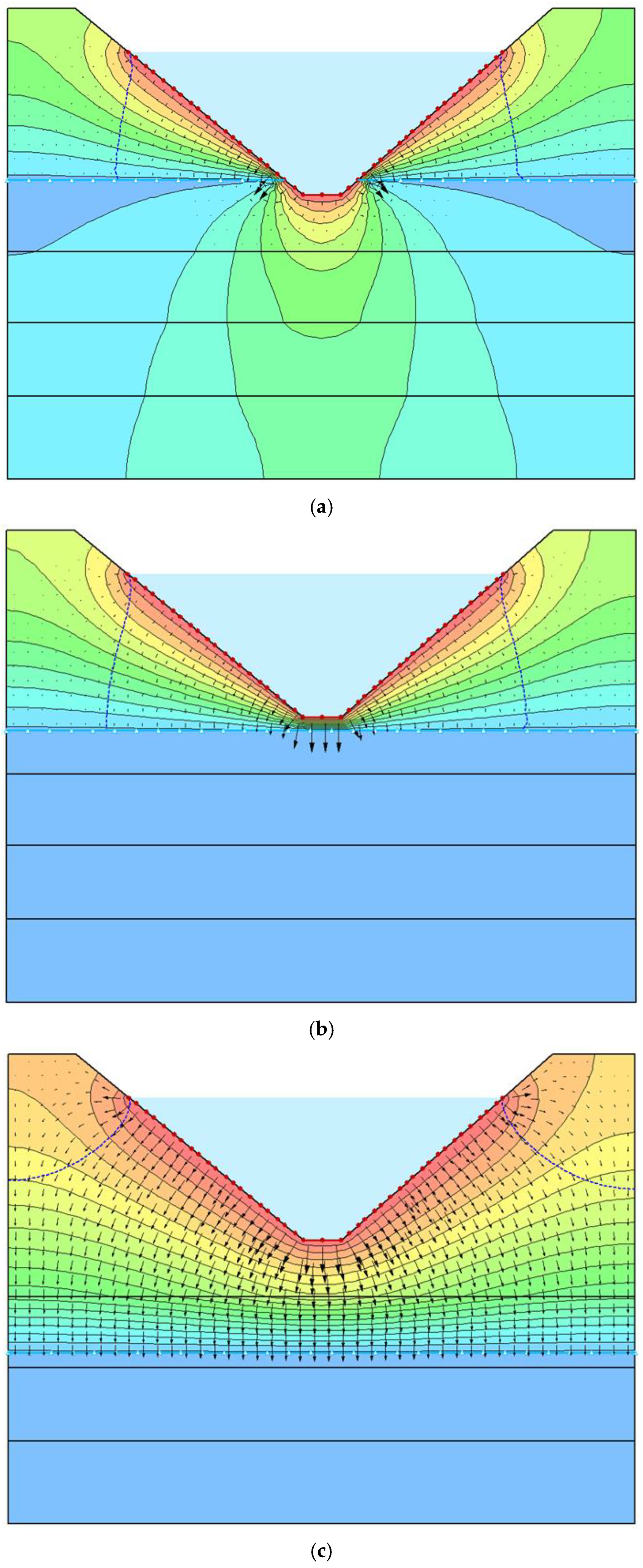
Figure 17.
Streamline directions and piezometric lines of the reservoir bottom. (a) Groundwater level above the reservoir bottom. (b) Groundwater level below the reservoir bottom (L = 5 m). (c) Groundwater level below the reservoir bottom (L = 40 m).
Figure 17.
Streamline directions and piezometric lines of the reservoir bottom. (a) Groundwater level above the reservoir bottom. (b) Groundwater level below the reservoir bottom (L = 5 m). (c) Groundwater level below the reservoir bottom (L = 40 m).

Figure 18.
Location of the Lianghekou power station.

Figure 19.
The dam body cross-section.

Figure 20.
The cross-section of the reservoir.

Figure 21.
A 3D FEM model of the clay core dam.

Figure 22.
Piezometric contours and water table in the dam body (y = 600 m).

Figure 23.
Piezometric contours and water table in the sub-base (x = 1018 m).


Table 1.
Each layer’s hydraulic conductivities and thicknesses.
| Layers | Thicknesses (m) | Hydraulic Conductivities (m/s) |
|---|---|---|
| Layer 1 | 20 | 1 × 10⁻⁶ |
| Layer 2 | 25 | 5 × 10⁻⁷ |
| Layer 3 | 27 | 1 × 10⁻⁷ |
| Layer 4 | 29 | 1 × 10⁻⁸ |
Table 2.
Leakage from the core.
| Position of Downstream Water Level Condition | Above the Reservoir Bottom | Below the Reservoir Bottom |
|---|---|---|
| H2 = 5 m | ||
| Analytical solution (m3/s) | 6.54 × 10⁻⁵ | 9.11 × 10⁻⁵ |
| Numerical solution (m3/s) | 6.02 × 10⁻⁵ | 8.47 × 10⁻⁵ |
| Absolute error (m3/s) | 0.52 × 10⁻⁵ | 0.64 × 10⁻⁵ |
| Relative error (%) | 7.95% | 7.03% |
Table 3.
Leakage from the bottom.
| Location of Groundwater Level Condition | Above the Reservoir Bottom | Below the Reservoir Bottom | |
|---|---|---|---|
| H1 = 5 m | L = 5 m | L = 40 m | |
| Analytical solution (m2/s) | 2.74 × 10⁻⁴ | 3.65 × 10⁻⁴ | 1.55 × 10⁻⁴ |
| Numerical solution (m2/s) | 2.51 × 10⁻⁴ | 3.33 × 10⁻⁴ | 1.41 × 10⁻⁴ |
| Absolute error (m2/s) | 0.23 × 10⁻⁴ | 0.32 × 10⁻⁴ | 0.14 × 10⁻⁴ |
| Relative error (%) | 8.39% | 8.77% | 9.03% |
Table 4.
Hydraulic conductivities of different zones of the dam body.
| Different Zones | Hydraulic Conductivities (m/s) |
|---|---|
| Core | 3.0 × 10⁻⁹ |
| Filter layer 1 | 2.47 × 10⁻⁵ |
| Filter layer 2 | 2.47 × 10⁻⁵ |
| Transition layer | 3.24 × 10⁻³ |
| Rockfill area 1 | 1.1 × 10⁻² |
| Rockfill area 2 | 1.1 × 10⁻² |
| Concrete floor | 5 × 10⁻¹⁰ |
| Grouting curtain | 3 × 10⁻⁷ |
Table 5.
Hydraulic conductivities of different layers of the rock-soil body.
| Different Layers | Hydraulic Conductivities (m/s) |
|---|---|
| q > 100 Lu | 1.3 × 10⁻⁴ |
| 10 Lu < q ≤ 100 Lu | 2.7 × 10⁻⁵ |
| 3 Lu < q ≤ 10 Lu | 3.2 × 10⁻⁶ |
| 1 Lu < q ≤ 3 Lu | 9.0 × 10⁻⁷ |
| q < 1 Lu | 1.3 × 10⁻⁷ |
Table 6.
Values of the corresponding parameters when the normal pool level is 2865.00 m a.s.l. and the downstream water level is 2610 m a.s.l.
Table 6.
Values of the corresponding parameters when the normal pool level is 2865.00 m a.s.l. and the downstream water level is 2610 m a.s.l.
| Parameters | Values |
|---|---|
| 282 m | |
| 27 m | |
| 27 m | |
| 29.5 m | |
| 621.7 m | |
| 29.5 m | |
| 153 m | |
| 56.4 m | |
| 96.6 m | |
| 40.2 m | |
| 20 m | |
| 78.69° | |
| 78.69° | |
| * | 42.27° |
| * | 45° |
* To simplify the calculation, the values of and are determined by averaging the slope of both sides of the core.
Table 7.
Leakage results calculated by both analytical and numerical methods.
| Leakage Area | Core | Reservoir Bottom | Total Leakage |
|---|---|---|---|
| Analytical solution (m3/d) | 196.54 | 6129.93 | 6326.47 |
| Numerical solution (m3/d) | 182.22 | 5593.14 | 5775.36 |
| Absolute error (m3/d) | 14.32 | 536.79 | 551.11 |
| Relative error (%) | 7.29% | 8.76% | 8.71% |
Publisher’s Note: MDPI stays neutral with regard to jurisdictional claims in published maps and institutional affiliations. |
© 2022 by the authors. Licensee MDPI, Basel, Switzerland. This article is an open access article distributed under the terms and conditions of the Creative Commons Attribution (CC BY) license (https://creativecommons.org/licenses/by/4.0/).
Share and Cite
MDPI and ACS Style
Yang, C.; Shen, Z.; Xu, L.; Shen, H. A Simplified Method for Leakage Estimation of Clay Core Dams with Different Groundwater Levels. Water 2022, 14, 1961. https://doi.org/10.3390/w14121961
AMA Style
Yang C, Shen Z, Xu L, Shen H. A Simplified Method for Leakage Estimation of Clay Core Dams with Different Groundwater Levels. Water. 2022; 14(12):1961. https://doi.org/10.3390/w14121961
Chicago/Turabian StyleYang, Chao, Zhenzhong Shen, Liqun Xu, and Hongjie Shen. 2022. "A Simplified Method for Leakage Estimation of Clay Core Dams with Different Groundwater Levels" Water 14, no. 12: 1961. https://doi.org/10.3390/w14121961
Note that from the first issue of 2016, this journal uses article numbers instead of page numbers. See further details here.