Article

Rainfall Runoff Balance Enhanced Model Applied to Tropical Hydrology

by
Arisvaldo Vieira Méllo Júnior
1,
Lina Maria Osorio Olivos
1,
Camila Billerbeck
1,
Silvana Susko Marcellini
2,
William Dantas Vichete
1,*,
Daniel Manabe Pasetti
1,
Ligia Monteiro da Silva
2,
Gabriel Anísio dos Santos Soares
2 and
João Rafael Bergamaschi Tercini
1
1
Departamento de Engenharia Hidráulica e Ambiental, Escola Politécnica, Universidade de São Paulo, São Paulo 05508-070, Brazil
2
Decision Support System Laboratory (LabSid), Escola Politécnica, Universidade de São Paulo, São Paulo 05508-070, Brazil
*
Author to whom correspondence should be addressed.
Water 2022, 14(12), 1958; https://doi.org/10.3390/w14121958
Submission received: 14 May 2022 / Revised: 5 June 2022 / Accepted: 7 June 2022 / Published: 18 June 2022
(This article belongs to the Special Issue Advances in Hydroinformatics for Water Data Management and Analysis)

Abstract

:
The integrative and comprehensive analysis considering the spatial and temporal representation of the hydrological process, such as the distribution of rainfall, land cover and land use, is a challenge for the water resources management. In tropical areas, energy availability throughout the year defines the rainfall distribution and evapotranspiration rate according to vegetation heterogeneity. To quantify water balance in tropical areas including these heterogeneities in the soil-vegetation-atmosphere relationship, we developed a fully distributed hydrological model called the Rainfall Runoff Balance Enhanced Model (RUBEM). The model was developed under a physics-based process structure, using remote sensing data to represent soil-water balance patterns, such as evapotranspiration, interception, baseflow, lateral flow, recharge, and runoff. The calibration procedure was based on nine global parameters. RUBEM could represent the spatio-temporal heterogeneities (soil, land use and land cover (LULC), topography, vegetation, and climate) in three basins in a tropical area. The results showed good adherence between the processes governing the soil-vegetation-atmosphere relationship according to the humidity indicator and the runoff coefficient. Overall, RUBEM can be used to help improve the management and planning of integrated water resources under climate, land use, and land cover changes in tropical regions.

1. Introduction

Understanding and quantifying hydrological patterns at the basin level under climate, land use, and land cover changes is a complex challenge [1,2,3]. Hydrological models play an important role in integrating water resource management (IWRM). These models have been developed since the 1960s [4]. The effects of the scientific community have led to the development of semi- and fully distributed hydrological models, such as VIC [5], SWAT [6], WetSpass [7], MGB-IPH [8], WEAP [9], SPHY [10], PCR-GLOBWB [11,12], MIKE-SHE [13,14,15,16,17], HIMS [18], IHDM [19], SLURP [20], the Xinanjiang Model [21], InHM [22], and PIHM [23], among others. The number of existing hydrological models is probably in the tens of thousands [24]. The US National Weather Service (NWS) has tested some of these models in the Distributed Model Intercomparison Project (DMIP) [25,26]. The DMIP showed that the performance of these models varies widely from good to very good and allows the application of current data input, such as radar rainfall and remote sensing data. In addition to the number of existing hydrological models, different conceptions and structural models contribute to understanding hydrological similarities and reducing the main source of uncertainties caused by model structure and specific pattern representation at the basin level [27,28,29,30,31].
The scale of application plays a vital role in determining flow patterns [32]. Heterogeneous small-scale features, such as vegetation, soil structure, preferential flow pathways through the soil, rills, and microtopography, are known to affect surface flow [4]. However, it is not guaranteed that the same equations will provide an excellent description of the physical flow process. Furthermore, the model parameters may not be suitable for representing basin mechanisms during the specified observation periods [33]. Hydrological responses are governed by the combination of climate, topography, soil, vegetation, and geology, which are the primary sources of heterogeneity in basins [34]. The accuracy of a model in representing physical processes depends on its ability to describe heterogeneities on an appropriate temporal and spatial scale [35].
In tropical areas, solar energy influences the hydrological cycle more directly than in other regions of the planet [1,36]. Rainfall is the main factor that determines seasons; therefore, the amount and time distribution of rainfall is an essential factor in distinguishing sub-climate zones as wet (>1800 mm), wet-dry (700–1800 mm), and dry (<700 mm) [37]. Based on the amount of energy available, evapotranspiration plays an essential role in determining water balance because of the link between the water and energy cycles on heterogeneous surfaces [38,39]. Currently, methodologies based on remote sensing are available to estimate evapotranspiration [40,41].
Along with climate change, other factors may also affect the hydrological cycle and watershed flow, such as changes in land use and land cover (LULC), construction of reservoirs, drainage systems, river morphology, agricultural practices, and significant increases in irrigation water [42,43]. All these factors alter the stability of the hydrological process at the basin level, thus affecting water resource management and planning.
Hydrological models capable of estimating basin hydrological pattern conditions based on physical processes are valuable tools for managing water resources [31,44]. These models are fundamentally crucial for watersheds that are deemed as critical owing to water scarcity or serious water conflicts, for predicting the response of unmonitored watersheds, and for planning future use based on land-use changes or climate change scenarios. Distributed hydrological models are usually parameterized by deriving the following parameter estimates: (i) topography, (ii) physical properties of the soils, and (iii) LULC in the basin [5,7,10,19].
Here, we present a distributed hydrological model called the Rainfall Runoff Balance Enhanced Model (RUBEM), which can compute the patterns of soil-water balance on a monthly time-step basis considering the observed rainfall and LULC changes throughout the simulation period. The formulation of the proposed model takes into account the monthly changes of LULC based on the remote sensing images to estimate the variable of the evapotranspiration process. The RUBEM limitations identified in the model development and the model application are: (i) fixed monthly time-step, (ii) depending on the watershed characteristics and input data spatialization, the minimum and maximum mean monthly discharge are underestimated, and (iii) knowledge of programing language data set input preprocessing. However, RUBEM is under development and allows improvements. Data set input pre-processing automatic applications are under development. Section 2 presents the methodologies applied for RUBEM development and the model applications to tree basins. Section 3 presents the results of the water cycle patterns, and Section 4 and Section 5 present the discussion and conclusions, respectively.

2. Materials and Methods
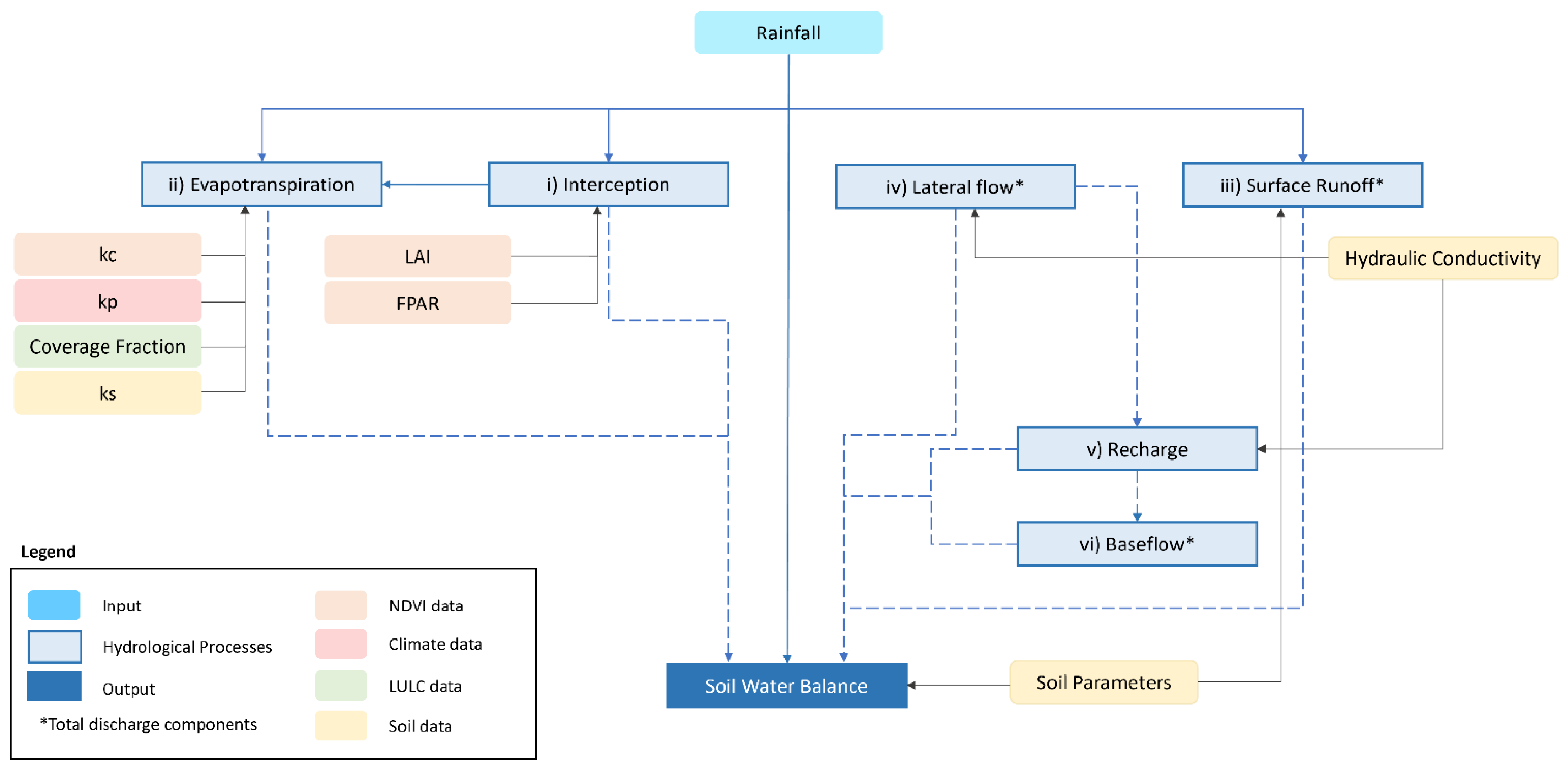
2.1. Model Overview

Hydrological models based on physical process structures have similar descriptions of formulation, scale, and solution technology. Physical processes rely on a set of variables and parameters organized into equations to simulate the response of hydrological patterns. These models are classified according to the level of detail in basin heterogeneity. The combined models do not consider spatial variability variables within the basin. Semi-distributed models reflect the spatial variability variables in sub-areas. Fully distributed models process spatial variability using grid cells [45].
In this paper, we present the RUBEM as a fully distributed hydrological model that integrates classical rainfall runoff processes [46]. Water balance formulation was based on [9,10,47]. Figure 1 shows the structure of the hydrological processes used in the model.
In tropical regions, evapotranspiration is one of the most important factors affecting the water balance physical process [36,48]. Evapotranspiration refers to the transfer of water from the soil-plant system to the atmosphere. Actual evapotranspiration is calculated based on the sum of evapotranspiration values for each land cover type using the concept of potential evapotranspiration [47]. The potential evapotranspiration ( E T p ) of the vegetated plot is calculated using the Penman-Montheith method [49]. To use the methodology described in [49], the crop coefficient ( k c ) and soil moisture reduction coefficient ( k s ) are calculated according to the N D V I (Normalized Difference Vegetation Index) and soil moisture content (Equations (1)–(5)).
E T R E A L = α V E T R , V + α S E T R , S + α W E T R , W + α I E T R , I
E T R , V = E T P k c k s
k c = k c m i n + ( k c m a x k c m i n ) ( N D V I N D V I m i n N D V I m a x N D V I m i n )
i f   N D V I   1.1 N D V I m i n   t h e n   k c = k c m i n
k s = l n ( T U R T U P M + 1 ) l n ( T U C C T U P M + 1 )
E T R , S = E T P k c m i n k s
i f   T U R < T U P M   t h e n   k s = 0
E T R , W = E T P k p
k p = 0.482 + 0.024 l n ( B ) 0.000376 U 2 + 0.0045 U R
E T R , I = I
where: E T R E A L —real evapotranspiration (mm); α V —vegetated fraction of cell area (%); α S —bare soil fraction of cell area (%); α W —water fraction of cell area (%); α I —impermeable fraction of cell area (%); E T R , V —real evapotranspiration of the vegetated area (mm); E T R , S —real evapotranspiration of the bare soil area (mm); E T R , W —real evapotranspiration of the water area (mm); E T R , I —real evapotranspiration of the impermeable area (mm); E T P —potential evapotranspiration (mm); k c —crop coefficient (-) ;   k c m a x and k c m i n —maximum and minimum possible values for crop coefficient; k s —soil moisture reduction coefficient (-); N D V I m a x and N D V I m i n —maximum and minimum values of the standardized vegetation index obtained based on the historical NDVI series for each cell; T U R —root zone moisture content (mm); T U P M —wilting point moisture content in the root zone (mm); T U C C —field capacity moisture content in the root zone (mm); k p —water evaporation coefficient (-); B —Class A Tank Border Width [between from 20 to 30 m] (m); U 2 —average wind speed at 2 m above ground surface (m/s); U R —relative humidity (%); and I —Interception [from 1 to 3 mm].
The coverage fractions and cell roughness coefficient were defined according to the coverage identification obtained from a previously classified raster image [50]. The value of the cover fraction is empirical and does not change during the analysis period; however, it can be modified according to the experience perception of the modeler. In the Supplementary Table S1 summarizes the values of cover fraction adopted in the model.
Crop water demand is a complex biological process that depends on soil moisture and the evaporative demand of the atmosphere [51,52]. The crop coefficient (kc) depends on the maximum and minimum values of vegetation and the NDVI under the following conditions: if NDVI ≤ 1.1 NDVImin, kc = kcmin. The soil moisture reduction coefficient (ks) depends on the moisture content. If the moisture content of the root area (TUR) is lower than the moisture content of the soil at the wilting point (TUPM), the coefficient of moisture reduction (ks) is zero. E T R , W depends on the water evaporation coefficient (Equation (8)), E T R , S is calculated using kcmin. E T R , w is calculated using the evaporation coefficient kp (Equation (9)), and E T R , I is based on the losses caused by interception (Equation (10)). Incorporating the processes of evapotranspiration and soil moisture content in the water balance process is important to represent heterogeneous sources, such as climate, rain, terrain, soil, and vegetation cover [34,35].
The water balance of soil is calculated in the non-saturated (root zone) and saturated zones (Equation (11)). The moisture content in the unsaturated zone depends on the previous moisture content, effective rainfall, and output (Equation (13)). Effective rainfall is the difference between the rainfall and interception in each cell (Equation (12)). The moisture of the saturated zone depends on the previous moisture, base flow, and groundwater recharge (Equation (S3)). A cell fully occupied by water with moisture in the root zone is considered saturated, that is, if α W = 1 then T U R = T U S .
In the root zone of the soil, surface runoff relies on soil moisture conditions based on lateral flow, recharge, and evapotranspiration. The saturated zone of the soil affects the calculation of base flow and recharge parameters. The water balance equation adopted in the RUBEM allows calculation of the total superficial flow.
T U R = T U R , T 1 + P E S R L F R E C E T R E A L
P E = P m I
T U S = T U S , T 1 B F + R E C
where T U R —root zone moisture content (mm); T U R , t 1 —root zone moisture content at the previous time step (mm); P E —effective precipitation (mm); S R —surface runoff (mm); L F —lateral flow (mm); R E C —groundwater recharge (mm); E T R E A L —total real evapotranspiration (mm); P m —total monthly precipitation (mm); I —total interception (mm); T U S —saturated zone moisture content (mm); T U S , t 1 —saturated zone moisture content at the previous time step (mm); and B F —base flow (mm).

2.2. Model Development

The model was written in Python using the PC Raster framework [53] to support the spatial calculation of water balance at the grid cell level. RUBEM is a continuous hydrological model with a formulation that represents the flow process between the soil and atmosphere layers. The model (i) integrates the main hydrological processes; (ii) has the flexibility to be applied for various applications, including climate and LULC change impact, irrigation planning, and drought; (iii) can be used for different spatial resolutions (pixel size options), applied to small and large watersheds, as well as at the farm and country levels; (iv) allow adequate representation of changes in land cover and related processes through monthly temporal resolutions; and (v) can be implemented easily. The implementation is open source, and the input and output maps can be directly used in Geographic Information System (GIS) environments; it uses remote sensing data, has a reduced number of parameters, and uses a configuration file that allows changing parameters and choosing the output. The RUBEM has six sets of data input: hydrological, climate, soil, ground elevation, LULC, and NVDI. Table 1 summarizes the model input data and their descriptions. Supplementary Figure S1 illustrates the water balance variables.
To assist the user in model application, we developed a plug-in for QGIS entitled RUBEM Hydrological, which supports the loading of input data, configures parameters, runs the model, and visualizes the results of the simulation. The plug-in does not have any preprocessing tools. However, the documentation and scripts for this purpose are openly available in the Supplementary Materials.

2.3. Model Aplication

The RUBEM was applied to three Brazilian basins, two of which are located in wet regions (Piracicaba River Basin (PRB) and Upper Iguaçu River Basin (UIRB)) whereas the third is located in the Brazilian semiarid region (Ipojuca River Basin (IRB)). The IRB has two hydrological zones with half of the region having a dry climate and the other half having a wet climate. The three basins present different characteristics of LULC, soil, evaporation, and hydrological regions (see details in the Supplementary Materials). Figure 2 shows the locations of the model application areas. The basins have different demands for water use, with primary needs for public supplies, industry, and agriculture, as shown in Table S6. The water abstraction and transposition system represents a challenge in the model calibration process under uncertainties from the observed gauge station and the natural runoff calculated using the applied methodology.

2.4. Calibration and Validation

A differential evolution algorithm [55] was used in the model calibration process. This method executes three operations: mutation, crossing and selection. The objective function was set to obtain a Nash –Sutcliffe efficiency (NSE) average value, for all station considered, close to N S E ¯ = 1. Over 27,000 combinations of the nine parameters were evaluated. For instance, the time required to choose solution in PRJ reached 120 h of processing. The selection criteria of the stations included a series with flaws, location in the basin, LULC, and rainfall regimes. The RUBEM calibration relies on nine global parameters, as listed in Table 2. Their range values were considered to represent the physical features of the watershed (soil, coverage, and rainfall). The values were based on [10,18,47], and verified on validation test in a subbasin of PRB.
From the 27,000 evaluation for each basin were selected the better sets of parameters, which resulted in the best NSE [56] according to Equations (S37) and (S38) (see Supplementary Materials), to verify the magnitudes of the water balance patterns. Thus, we evaluated whether the parameters of evapotranspiration and recharge flows in the river were consistent with the proportions reported in [10,47,57,58]. The set that results in the best combination of NSE and water balance proportions consistency were select as final calibrated parameters.
In addition to the calibration process assessment, we also evaluated the root mean square error (RMSE) using Equation (S36) [44]; number of times the variability of the observations was greater than the mean error—nt nd relative bias—RB using Equation (S39) [59]; and the asynchronous regression method that determines the function F ( Q s ) = u ƃ F ( Q o ) according to the percentiles of qo and qs of the distribution of F ( Q o ) and F ( Q s ) at each probability level using equations from Equations (S40)–(S42) [60]. Table S4 presents the criteria used for evaluating the performance indicators as described in [56,61].

3. Results

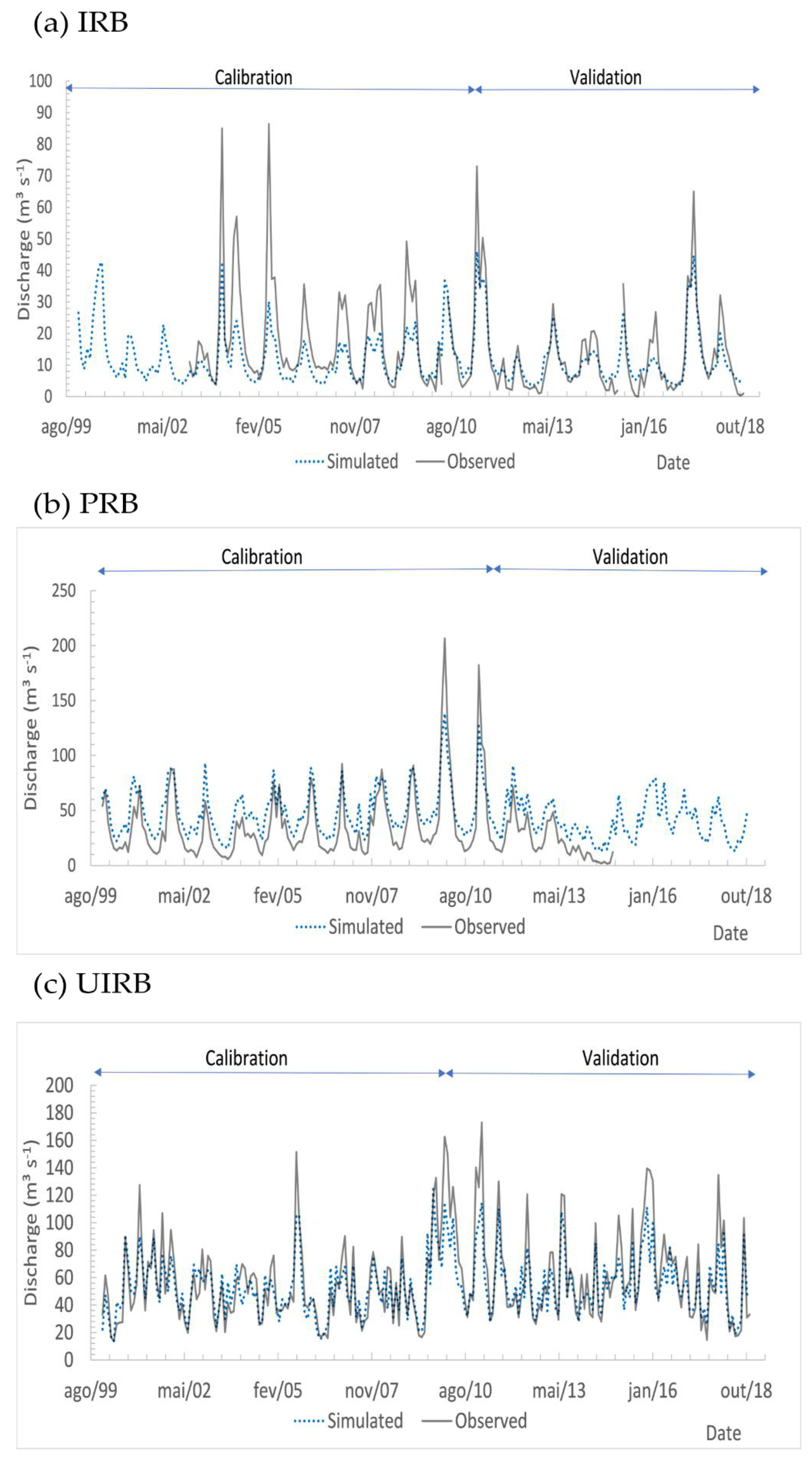
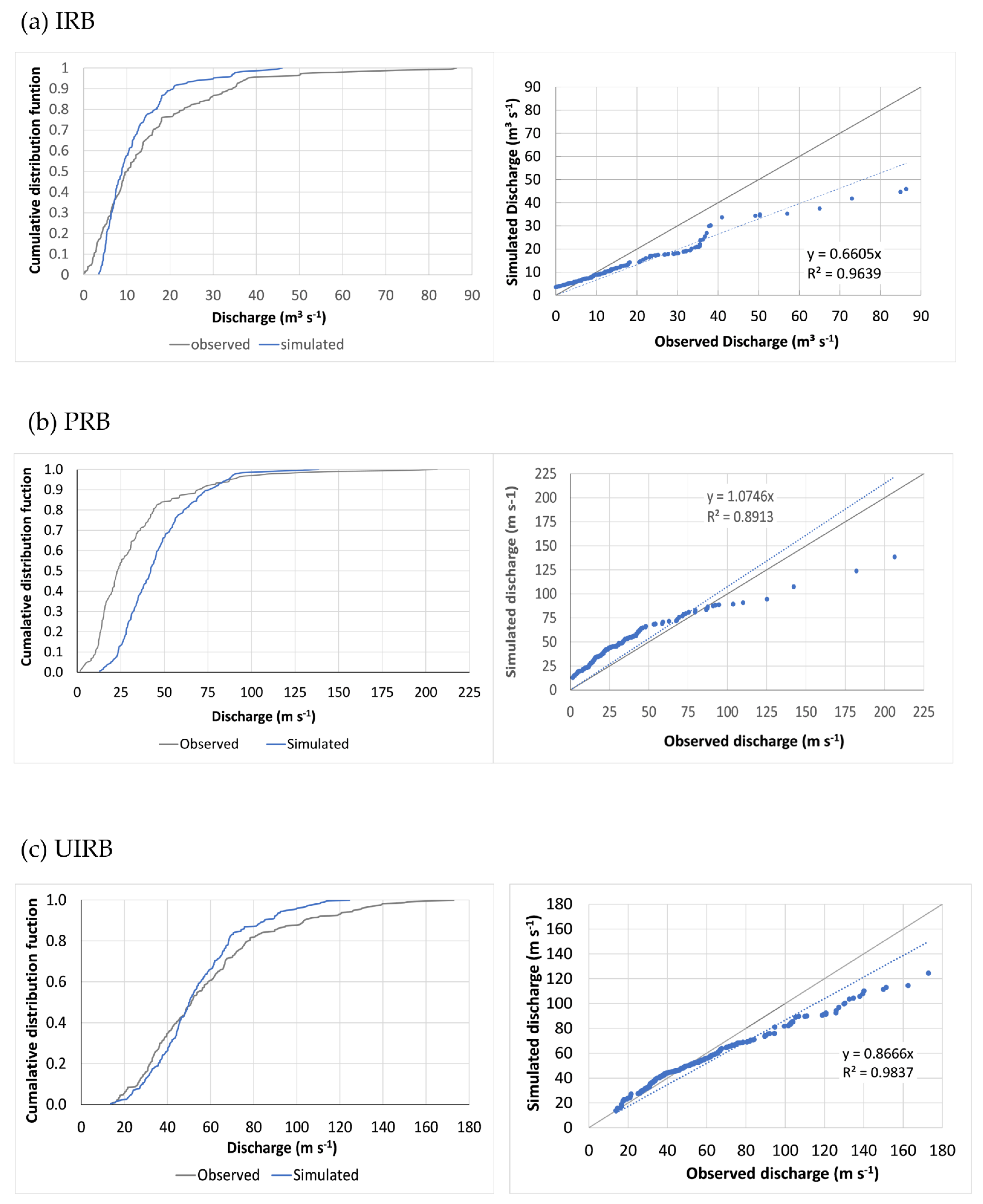
3.1. Calibration and Validation

The modeled results were evaluated for the calibration period (January 2000 to December 2009) and the validation period (January 2010 to December 2018). At least five stream gauges were considered for each basin in the calibration process. Global parameters obtained during the calibration process were applied during the validation period. Table 3 shows the values for each of these parameters in the three basins. Figure 3 shows the hydrographs for the calibration and validation periods.
Table 4 lists the model efficiency indices (RMSE, NSE, and RB) for the three basins of the model application. The RMSE was acceptable or good at most of the gauge stations in the three basins during the two periods analyzed. Ref. [62] assumed that RMSE values below half of the standard deviation (SD) for the observed flows can be considered low. This criterion was met at all gauge stations during both analysis periods.
The number of times (nt) when the variability of the observations exceeds the average error allows us to assess the representativeness of the range covered by the simulated values [56]. Thus, the performance of the model does not change linearly with the NSE. The NSE was unsatisfactory for the IRB during calibration in two gauge stations (15.7% of the drainage area) at UIRB and in five gauge stations (80.91%) at the PRB. During the validation period, the NSE was acceptable or good in three gauge stations (71.3% of the area) at the IPR, five (72.2%) at the PRB, and three (84.3%) at the UIRB.
The RB measures the relationship between the average error and average flow observed [59]. The RB was unsatisfactory in the IRB, resulting in higher calibration values. In the PRB, bias was equal to or greater than acceptable at three gauge stations in calibration and at four validation stations. In the UIRB, good or very good levels were observed in both periods, and a slight negative bias prevailed (Table 4).
The hydrographs are presented at the most significant drainage areas for each of the basins of the model application. The IRB (Figure 3a) shows that the model underestimated the highest discharges and adjusted the lowest discharges during the calibration period, resulting in RB = −0.397. The model was thus suitable for both high and low discharges (RB = 0.007). In the PRB (Figure 3b), the model overestimated the low discharges and adjusted them to high discharges in both periods, yielding RB = 0.468 (calibration) and RB = 0.348 (validation). In the UIRB (Figure 3c), all index performances for both periods were considered satisfactory.
Efficiency indices use simultaneous observations and simulations of flow data. Small sample sizes limit the representativeness of efficiency indicators [56,59]. Ref. [60] proposed a regression of one time-varying quantity against another without requiring simultaneous knowledge of both. Asynchronous regression was performed with the observed and simulated discharges related to the percentile of their accumulated distribution, as shown in Figure 4. The proximity of cumulative distribution indicated the model performance. The model did not reproduce the highest discharge in the three basins. The asynchronous regression results R2 > 0.89 for all basins, but the modified regression coefficient (rm) considering the sum of squared deviations from the respective averages are low [63]. The model tended to underestimate flows in the IRB (rm = 0.30) and UIRB (rm = 0.46) basins and to underestimate in the PRB (rm = 0.49). The fitted line was effective for comparing the 1:1 ratio between the observed and simulated discharges. Fisher’s test of the two samples, considering the indifference of the mean and variance between the samples, indicated no significant difference (99% confidence) between the observed and simulated flows in the three basins. Ref. [64] considered a satisfactory fit for R2 = 0.72 in simulations of the Brazilian basin. Ref. [65] show the good correlation between modelled and observed base flow index (R2 > 0.87).
The results showed a good fit for calculating the average monthly discharge for all periods (from January 2000 to December 2018). RUBEM underestimated the median discharges by 23.5% in the wet season and 9.3% in the dry season in the IRB. In the PRB, the median discharge was overestimated by 33.7% and 51% during the wet and dry seasons, respectively. In the UIRB, the model underestimated the median discharge by 8.1% during the wet season and 4.3% during the dry season.

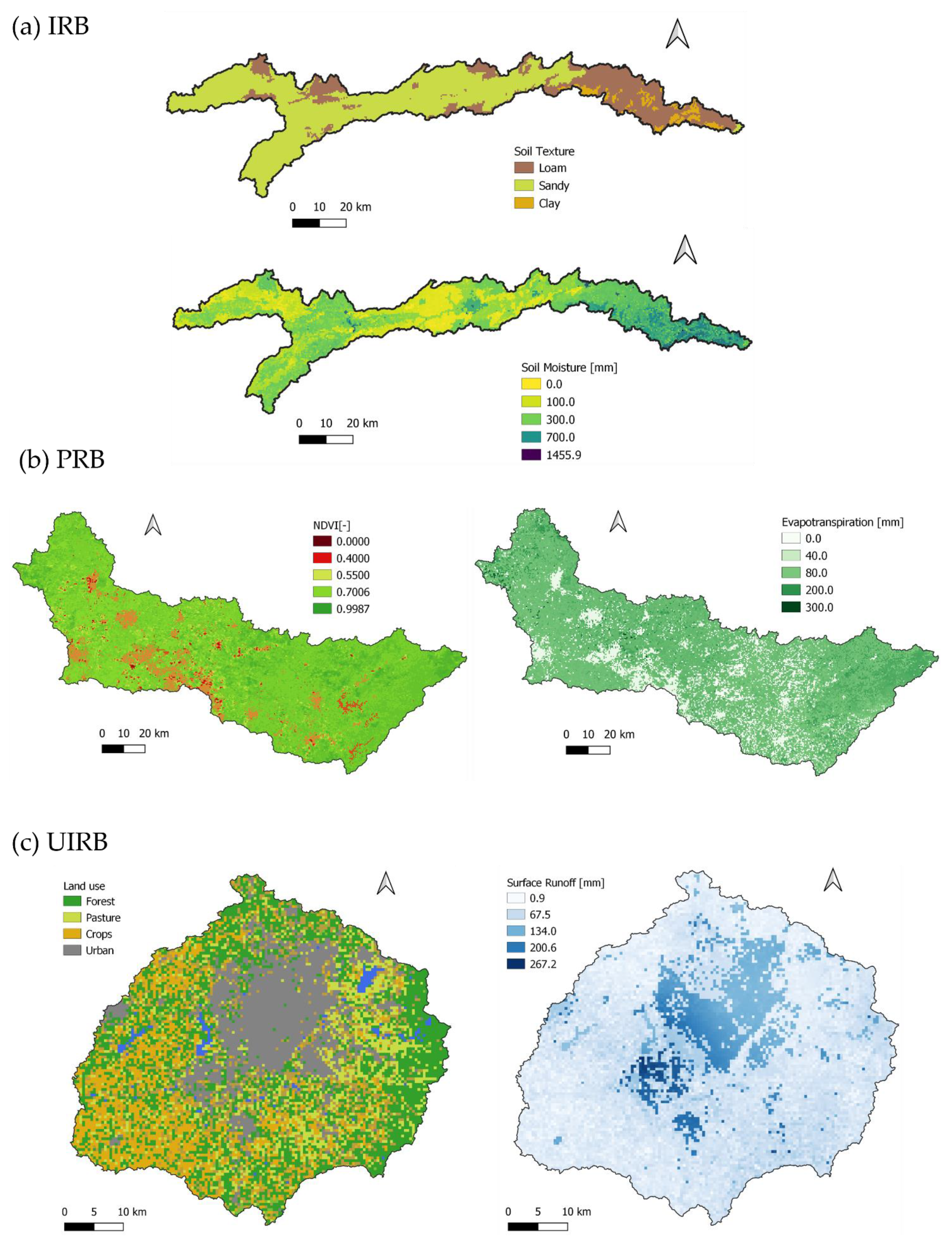
3.2. Soil and LULC Heterogeneities Analysis

The entire output parameter has spatial-temporal results as a raster file. Figure 5 shows lower evapotranspiration in areas with low NDVI values, more significant moisture in the soil texture of loam and clay, and higher impervious areas and surface runoff in urban land use. All spatially calculated variables are shown in Figures S11–S13 (Supplementary Materials).
With a suitable performance of the model application results, water balance patterns during the calibration and validation periods could be evaluated according to the observed rainfall and LULC through spatial-temporal changes. Three cells were selected to evaluate the LULC modifications throughout the simulation period (Figure 6). The evaluated patterns were compared with the total rainfall to compute the ratio of each component in the three cells. Cell 1 (−8.33 lat, −35.20 long) presents a pasture area that turns into a forest area in the IRB. Cell 2 (−22.58 lat, −47.68 long) shows an area without LULC changes in the PRB, and Cell 3 (−25.54 lat, −49.40 long) shows an area that began as a forest, changed to a pasture, back to a forest, followed by cropland, and changed into an urban area in the UIRB. The forest cover in the IRB and UIRB constitutes the Atlantic Forest ecosystem. The NDVI (from 0.23 to 0.83) and kc (from 1.14 to 1.8) extensions were greater in UIRB than in IRB (NDVI from 0.53 to 0.89 and kc from 1.46 to 1.8).
The area with no alterations in the LULC in the simulation period resulted in a comprehensive pattern of the soil-water balance as expected, regarding the antecedent soil moisture conditions, meaning that the pattern had a standard pattern for each component. However, altered LULC resulted in significant changes in the water cycle patterns. Figure 6 shows the water cycle patterns for the selected cell. For instance, in the IRB sample, interception of the coverage area with the forest was significantly higher and evapotranspiration was slightly lower than that in the period in which the cell was cropped. In the PRB, evapotranspiration was significantly higher, with 65% of the rainfall occurring in 2014. A change in the LULC from the crops to urban areas in the last UIRB period resulted in an increase in surface runoff from 40% to 77% of the rainfall, and evapotranspiration from 62% with forest cover to 47% with crop cover and 7% with urban cover. The cell shows that the difference in evapotranspiration corresponds to nearly 60% of precipitation in 2000 (forest cover), approximately 10% between 2016 and 2018 (urban cover), and approximately 10% from 2016 to 2018 (urban cover), while the runoff was 30% and 80%, respectively.
The correlation between the moisture index (P/ETp) and runoff coefficient (SR/P) was verified for a set of cells with different coverages [66], randomly selected in the three basins (IRB = 320; PRB = 1000 and UIRB = 250) in a month representing the wet (Figure 7a) and dry seasons (Figure 7b). The correlation coefficients for the wet (r = 0.71) and dry (r = 0.66) seasons indicate a satisfactory approach [65,67] for the spatial (500 m grid) and temporal (monthly) scales to represent the relationship between water availability and runoff. The correlations between P/ETp and SR/P in the cells sampled with equal coverage in the basins showed a strong correlation in both seasons (Table 5).

4. Discussion

4.1. Calibration and Validation

We understand that changes in soil saturation significantly impact the patterns of base flow and runoff, supported by the minimum and maximum annual total rainfall. Higher specific rainfall events did not have a high impact on recharge, evapotranspiration, or base flow, which were directly related to the soil-water balance layer. Generally, application of the model is considered acceptable. However, Figure 3 shows that RUBEM was unable to simulate the highest mean monthly runoff, possibly because the highest rainfall event could modify the mean monthly runoff but could not change the soil balance according to the temporal scale. Furthermore, the poorer quality flow record and anthropogenic act amplify the differences between the series. However, the index performances show that the model were considered satisfactory, according to [64,65,67].
The interception parameter was significantly higher in the UIRB (α = 9.77), indicating greater interception of rainfall in this basin. The RCD and w2 values were higher in the UIRB (RCD = 8.34; w2 = 0.43) and PRB (RCD = 7.96; w2 = 0.35). These parameters contribute to increasing the potential runoff in permeable areas. In the IRB, the parameters RCD = 5.38, w2 = 0.12, and low soil moisture factors (b = 0.08) reduced surface runoff. The largest area of the IRB in the semiarid region explains this parameter value.
The highest value of the factor for the partition of flow directions in the PRB (f = 0.77) and UIRB (f = 0.83) favored lateral flow and did not favor recharge in these basins. Recharge plays a vital role in forming the basic flow, particularly during long dry months [10,47,61]. The higher value of the basic flow recession factor observed in the IRB (αgw = 0.92) disfavors basic flow, a feature of arid regions. Higher values of the damping coefficient increased the importance of the discharge generated in the previous month and reduced the discharge generated in each cell in the current month. This coefficient was the highest in the IRB (x = 0.31), resulting in a more significant damping of discharge into the basin.
The same set of parameters controlled all drainage processes during the analysis period. This condition facilitates representation of soil, climate, cover heterogeneities, and calibration of the best parameter sets. Manual calibration is also possible [10,47,58], but is very laborious. The differential evolutionary algorithm adopted in this study was proven to be effective. However, high levels of heterogeneity may hinder parameter calibration. As most IRBs are in dry regions and the other regions are wet, RUBEM performance was poor.
We considered the representative parameter sets to simulate the discharge in each basin for calibration and validation. RMSE, NSE, RB, and asynchronous regression showed acceptable results. Even though the NSE obtained in the calibration was unsatisfactory for the IRB, it was acceptable or good in the largest basin area during the validation period. The same behavior was observed for the UIRB and PRB. Considering the downstream gauge station, simulation discharges were lower than those observed 60% of the time in the IRB and UIRB and were higher than those observed 92% of the time in the PRB. However, the regression coefficients between the observed and simulated discharges were satisfactory for all three basins.
Asynchronous regressions between cumulative distributions of observed and simulation discharges can be used to fill the missing data in observed datasets, hindcast studies, as well as forecast discharges based on rainfall estimates from regional climate models for ungauged areas [68,69,70].
The NSE was acceptable for UIRB and unsatisfactory for IRB and PRB during the calibration period [71]. Some characteristics of the study areas were determinants of the results obtained. The basins supply water to cities and have an important water demand for different uses. The PRB and UIRB present reservoir systems for supply systems. In the PRB, four of the seven-gauge stations used for calibration are affected by a considerable transfer of water to a neighboring basin. The difference between the observed and natural simulated discharges contributed to the reduction in NSE during the calibration. The results of the gauges located in the upper basins with low anthropogenic interference (Supplementary Figure S8) showed better NSE and index results (acceptable according to Supplementary Table S4). According to [72], global calibration is limited to homogeneous hydrological regimes and implies a diminution in performance, specifically in estimating high flows in small catchments. The two opposite rainfall regimes at the IRB (semiarid and wetland) suggest that it is necessary to consider two sets of different parameters for calibration. During the validation period, NSE was acceptable or good in all three basins. The RB was very good for the UIRB during calibration and for the IRB during validation. Discharges were overestimated in the PRB and underestimated in the IRB and UIRB.
Asynchronous regression represents a linear regression between the observed and simulated flow duration curves. The hydrograph of the observed and simulated monthly discharge shows a good recession shape. The median, mean, maximum, and minimum monthly discharges were also evaluated in the results and discussion.
RUBEM showed different results in the smaller drainage areas of the three basins. The worst performance was found at a 672 km2 gauge station in the IRB basin. Wang et al. 2018 achieved a moderate performance in basins smaller than 400 km2 because of the solid nonlinear relationship between rainfall and flow. Ref. [47] found that the WetSpass model failed in small basins because some processes involved had timescales shorter than a month.
In the three basin simulations, the grid resolution was set at 500 m. RUBEM was tested in a 55.6 km2 PRB sub-basin with a grid resolution of 30 m and showed satisfactory performance. A greater spatial resolution provides more details on the variables influencing runoff. However, this increases the number of variables, simulation computational burden, and difficulty in calibrating the parameters. Therefore, the spatial scale is defined based on the degree of variability and uncertainty to be represented. Refs. [4,35,62,73] pointed out that the model does not represent the heterogeneity of microscale hydrological processes, even at a large spatial resolution.
The physical characteristics of the soil in each basin also varied, resulting in uncertainty. The values adopted for each basin represent the average conditions according to the classification adopted in Brazil [54]. As in the VIC model [73], RUBEM also demonstrated sensitivity in adjusting minimum flows under specific conditions of long-term dry periods. Under these conditions, better model adaptability can be achieved by improving the physical and hydrological properties of soil.
RUBEM was developed to improve the management and planning of integrated water resources under climate, land use, and land cover changes in tropical areas. The time step to represent hydrological process according to the model formulation at a grid basis level was selected according to the time-scale response of the soil recharge and evapotranspiration processes [74], including the hydrometric gauge station quality in Brazil [64,75]. Furthermore, we noted the successful application of the SWAT model (semi-distributed) in Brazilian watersheds, with very good calibration results on a monthly basis rather than on a daily basis [76]. However, RUBEM has been developed using a physics-based process description structure [28,77,78] and remote sensing data [3,50] to improve the soil-water balance (evapotranspiration, interception, baseflow, and recharge) in tropical regions. Different conceptions and structural models contribute to understanding hydrological similarity and reducing the main source of uncertainties introduced by the model structure and specific pattern representation at the basin level [27,28,29,30,31]. Additionally, it is important to note the uncertainties and accuracy of the input dataset, especially the hydrometrical gauge stations, which have one of the most important roles in the calibration and validation modelling assessment.

4.2. Soil and LULC Heterogeneities

The volume of moisture available in the root layer is influenced by depth, thickness, bulk density, and moisture content. The depth of soil to be explored by the root system of vegetation is defined by the physical properties of the soil class. This ensures that the water capacity of the soil is not limited by the depth of the root system. Although the different vegetation types present different root system characteristics, removal of water from the soil by the plant is estimated by ETREAL, which depends on the type of physio-morphological characteristics of the vegetation in each cell. The kc and ks define the removal of water from soil. According to [49], the ET of a species can be obtained using empirical values of kc, which should include all the differences in the physiological morphology of the crop in its real state and the potential conditions (soil-water availability, leaf mass, and full physiological activity).
In distributed hydrological models, different responses are expected at different temporal and spatial scales. The correlation between the climatological and physical characteristics of the basin helps understand the prevailing controls on the behavior of the basin at a particular scale [66]. The correlation between the moisture index (P/ETp) and runoff coefficient (SR/P) at specific spatial and temporal scales was found to assess the representativeness of the analysis. Cell sampling during the dry season resulted in a very low average P/ETp in the UIRB, indicating that the month sampled (July 2018) was very dry, resulting in a low SR/P. Located in the same hydrological region, the PRB showed an average P/ETp 11 times higher than that obtained in the UIRB in the sampled month (June 2013), resulting in an SR/P twice as high. The antecedent storage of water in the soil at the UIRB may have been the cause of this disproportionation. The P/ETp anomaly during the dry month of the UIRB contributed to a reduction in the correlation coefficient between the indices. The IRB presented P/ETp in the wet season that was three times greater than that in the dry season (February 2014), resulting in a proportional reduction of SR/P. This basin is located at a higher latitude, with a high atmospheric evaporative demand in the season and shallower soil. The correlations for crops, agriculture, and pasture were lower due to differences in responses in the UIRB and PRB. At the UIRB, the species showed lower water demand (kc = 0.66), and many species had a short development and production cycle in the wet season, including temperate vegetable and fruit crops between sprouting and harvesting, resulting in lower evapotranspiration. In the PRB, the species demanded more water (kc = 0.69). The predominant species in this basin is sugarcane, which has a longer development period and greater water consumption. Ref. [57] found P/ET = 2.27 in a sub-basin of the PRB in 35.5% of the forests and 31% of the pastures. Refs. [58,61] achieved a ratio of 1.14 in Africa and 1.63 in a basin in western São Paulo, respectively.
RUBEM estimates ETREAL using the average ETp data, kc based on NDVI, and ks using soil-water balance. Figure 4 and Figure 5 show the consistency in estimating these variables. The magnitudes of the hydrological components of the cycle were compared with the results presented in literature. Thus, evapotranspiration and soil moisture values were estimated to correspond to the results of multiple studies that used remote sensing in Brazil [79,80,81].
The linear regressions between kc and NDVI for the cells shown in Figure 8 showed r > 0.99 for all vegetation cover. The higher NDVI for the forest was consistent with the kc values in relation with other coverages. [82,83] observed a strong kc-NDVI correlation for crops and pastures at different stages of development. [83] observed a lack of sensitivity of NDVI at high Leaf Area Index (LAI) values. This means that both plant transpiration and light absorption increase at roughly the same rate at low LAI and then saturate. Consequently, kc adjusts better for high NDVI and underestimates for low NDVI.
The highest kc for forests indicates greater consumption of water than that observed for crops and pastures. Ref. [84] observed an LAI of 5.8 to 7.8 m2 m−2 for the Atlantic Forest in Brazil. Although transpiration is positively correlated with LAI, radiation attenuation from the top of the canopy to the lower parts brings the global conductance of several forest species very close for LAI > 3 m2 m−2. However, an increase in LAI implies greater interception and consequent evaporation of water accumulated in the canopy. During periods of water scarcity and lower irradiance, absorption of water from the soil occurs at greater depths. The root system of Atlantic Forest species can reach up to 5 m [84]. According to [49], stomatal resistance increases with plant growth and maturation, under water stress conditions, and restriction of water availability in the soil, thus limiting the ETREAL. Ref. [85] observed that water stress conditions increased stomatal resistance, reaching triple its value in tropical forests.
The ETREAL formulation recognizes changes in vegetation over time through the NDVI, but does not consider stomatal resistance, and does not distinguish physiological differences between plant species. However, the formulation adopted for estimating the LAI, kc, and moisture content in the root zone was considered satisfactory for calculating the soil-water balance and ETREAL under different climatic conditions and vegetation cover. The soil layer water balance is the most important representation of water cycle patterns to understand the impact of LULC changes because of anthropic land use and planning.
Sensitivity analyses of input variables in the WetSpass model show that the critical factors are precipitation, LAI, and potential evapotranspiration [47]. RUBEM satisfactorily represented the changes in LULC. In two cells with and in one without coverage changes, the model calculated the variables proportionally according to the changes over time.
The model source code was written in the Python programming language, and the PCRaster library dynamic model framework was used to perform spatial calculations. The LULC simulation used the NDVI time series to change over time. The root depth remained constant throughout the simulation period, and there were no snow-melting equations.

5. Conclusions

RUBEM input data and formulation are intended to represent variables that impact the physical processes of the hydrological cycle (on which RUBEM is based). Thus, NDVI from remote sensing data tends to cover the characteristics of plant species, such as stomatal resistance. The model also captures a constant pattern of recharge, evapotranspiration, and runoff in a covered area without LULC changes, with respect to precipitation changes that could affect the soil moisture conditions.
The RUBEM formulation has a specific physics-based structure to represent changes in water balance patterns represented by spatio-temporal heterogeneity variables. Overall, RUBEM can be used to help improve the management and planning of integrated water resources under climate, land use, and land cover changes in tropical regions.

Supplementary Materials

The following supporting information can be downloaded at: https://www.mdpi.com/article/10.3390/w14121958/s1, Supplementary archive. References [86,87,88,89,90,91,92,93,94,95,96,97,98,99,100,101,102,103,104,105,106,107,108,109,110,111,112,113,114,115,116,117,118,119,120,121,122,123,124,125,126,127] are citied in the Supplementat Materials.

Author Contributions

Model Conceptualization A.V.M.J., L.M.O.O., C.B., S.S.M. and W.D.V.; Software: G.A.d.S.S., L.M.O.O., W.D.V., C.B. and D.M.P.; Data collection and organization: L.M.d.S., L.M.O.O., C.B. and S.S.M.; writing—original draft preparation A.V.M.J., W.D.V., J.R.B.T. and D.M.P.; writing—review and editing: S.S.M. and L.M.d.S.; project administration: A.V.M.J.; funding acquisition: A.V.M.J., G.A.d.S.S. and L.M.d.S. All authors have read and agreed to the published version of the manuscript.

Funding

This research was funded by Fundo Amigos da Poli, grant number 2020-043.

Institutional Review Board Statement

Not applicable.

Informed Consent Statement

Not applicable.

Data Availability Statement

The data that support the findings of this study are openly available in Hydroshare at https://doi.org/10.4211/hs.6f3670b8cd944e7ea72e03d1b9ca928f (create date 21 October 2021). Also, the RUBEM documentation and source code are openly available at https://rubem-hydrological.readthedocs.io (2021) and https://github.com/LabSid-USP/RUBEMHydrological#readme respectively.

Acknowledgments

We appreciate the “Fundo Amigos da Poli” by the source of funds for model development, and Rubem La Laina Porto (in memoriam) for their efforts and contributions in the Brazilian Water Resource community.

Conflicts of Interest

The authors declare no conflict of interest and the funders had no role in the design of the study, analyses, interpretation of data and in the writing of the manuscript.

References

  1. Garg, V.; Nikam, B.R.; Thakur, P.K.; Aggarwal, S.P.; Gupta, P.K.; Srivastav, S.K. Human-Induced Land Use Land Cover Change and Its Impact on Hydrology. HydroResearch 2019, 1, 48–56. [Google Scholar] [CrossRef]
  2. Pokhrel, Y.; Burbano, M.; Roush, J.; Kang, H.; Sridhar, V.; Hyndman, D. A Review of the Integrated Effects of Changing Climate, Land Use, and Dams on Mekong River Hydrology. Water 2018, 10, 266. [Google Scholar] [CrossRef] [Green Version]
  3. Fendrich, A.N.; Barretto, A.; de Faria, V.G.; de Bastiani, F.; Tenneson, K.; Guedes Pinto, L.F.; Sparovek, G. Disclosing Contrasting Scenarios for Future Land Cover in Brazil: Results from a High-Resolution Spatiotemporal Model. Sci. Total Environ. 2020, 742, 140477. [Google Scholar] [CrossRef]
  4. Woolhiser, D.A. Search for Physically Based Runoff Model—A Hydrologic El Dorado? J. Hydraul. Eng. 1996, 122, 122–129. [Google Scholar] [CrossRef] [Green Version]
  5. Liang, X.; Lettenmaier, D.P.; Wood, E.F.; Burges, S.J. A Simple Hydrologically Based Model of Land Surface Water and Energy Fluxes for General Circulation Models. J. Geophys. Res. 1994, 99, 14415–14428. [Google Scholar] [CrossRef]
  6. Neitsch, S.L.; Arnold, J.G.; Kiniry, J.R.; Williams, J.R.; King, K.W. Soil and Water Assessment Tool (SWAT) User’s Manual, Version 2000, Grassland Soil and Water Research Laboratory. Texas Water Resour. Institute Coll. Stn. 2002, 13, 52–55. [Google Scholar]
  7. Batelaan, O.; De Smedt, F. WetSpass: A Flexible, GIS Based, Distributed Recharge Methodology for Regional Groundwater Modelling. In Impact of Human Activity on Groundwater Dynamics; Gehrels, H., Peters, N.E., Hoehn, E., Jensen, K., Leibundgut, C., Griffioen, J., Webb, B., Zaadnoordijk, W.J., Eds.; IAHS Publication 269; IAHS Press: Wallingford, UK, 2001; pp. 11–18. ISBN 1-901502-56-2. [Google Scholar]
  8. Collischonn, W.; Allasia, D.; da Silva, B.C.; Tucci, C.E.M. The MGB-IPH Model for Large-Scale Rainfall-Runoff Modelling. Hydrol. Sci. J. 2007, 52, 878–895. [Google Scholar] [CrossRef] [Green Version]
  9. Yates, D.; Sieber, J.; Purkey, D.; Huber-Lee, A. WEAP21—A Demand-, Priority-, and Preference-Driven Water Planning Model. Part 1: Model Characteristics. Water Int. 2005, 30, 487–500. [Google Scholar] [CrossRef]
  10. Terink, W.; Lutz, A.F.; Simons, G.W.H.; Immerzeel, W.W.; Droogers, P. SPHY v2.0: Spatial Processes in HYdrology. Geosci. Model Dev. 2015, 8, 2009–2034. [Google Scholar] [CrossRef] [Green Version]
  11. Bierkensi, M.F.P.; Van Beek, L.P.H. Seasonal Predictability of European Discharge: NAO and Hydrological Response Time. J. Hydrometeorol. 2009, 10, 953–968. [Google Scholar] [CrossRef]
  12. Sperna Weiland, F.C.; Van Beek, L.P.H.; Kwadijk, J.C.J.; Bierkens, M.F.P. The Ability of a GCM-Forced Hydrological Model to Reproduce Global Discharge Variability. Hydrol. Earth Syst. Sci. 2010, 14, 1595–1621. [Google Scholar] [CrossRef] [Green Version]
  13. Abbott, M.B.; Bathurst, J.C.; Cunge, J.A.; O’Connell, P.E.; Rasmussen, J. An Introduction to the European Hydrological System—Systeme Hydrologique Europeen, “SHE”, 2: Structure of a Physically-Based, Distributed Modelling System. J. Hydrol. 1986, 87, 61–77. [Google Scholar] [CrossRef]
  14. Abbott, M.B.; Bathurst, J.C.; Cunge, J.A.; O’Connell, P.E.; Rasmussen, J. An Introduction to the European Hydrological System—Systeme Hydrologique Europeen, “SHE”, 1: History and Philosophy of a Physically-Based, Distributed Modelling System. J. Hydrol. 1986, 87, 45–59. [Google Scholar] [CrossRef]
  15. Refshaard, J.C.; Storm, B. MIKE SHE. Comput. Model. Watershed Hydrol. 1995, 3, 809–846. [Google Scholar]
  16. Oogathoo, S.; Prasher, S.O.; Rudra, R.; Patel, R.M. Calibration and Validation of the MIKE SHE Model in Canagagigue Creek Watershed. In Agricultural and Biosystems Engineering for a Sustainable World, Proceedings of the International Conference on Agricultural Engineering, Hersonissos, Greece, 23–25 June 2008; European Society of Agricultural Engineers (AgEng): Silsoe, UK, 2008. [Google Scholar]
  17. Shukla, M. Soil Hydrology, Land Use and Agriculture: Measurement and Modelling; CABI: Wallingford, UK, 2011; ISBN 978-1-84593-877-2. [Google Scholar]
  18. Wang, L.; Wang, Z.; Liu, C.; Bai, P.; Liu, X. A Flexible Framework Hydroinformatic Modeling System-HIMS. Water 2018, 10, 962. [Google Scholar] [CrossRef] [Green Version]
  19. Beven, K.; Calver, A.; Morris, E.M. The Institute of Hydrology Distributed Model; Report 98; Ministry of Agriculture, Fisheries and Food: Wallingford, UK, 1987.
  20. Kite, G.W.; Kouwen, N. Watershed Modeling Using Land Classifications. Water Resour. Res. 1992, 28, 3193–3200. [Google Scholar] [CrossRef]
  21. Ren-Jun, Z. The Xinanjiang Model Applied in China. J. Hydrol. 1992, 135, 371–381. [Google Scholar] [CrossRef]
  22. Van der Kwaak, J.E.; Loague, K. Hydrologic-Response Simulations for the R-5 Catchment with a Comprehensive Physics-Based Model. Water Resour. Res. 2001, 37, 999–1013. [Google Scholar] [CrossRef]
  23. Qu, Y.; Duffy, C.J. A Semidiscrete Finite Volume Formulation for Multiprocess Watershed Simulation. Water Resour. Res. 2007, 43, 5752. [Google Scholar] [CrossRef]
  24. Droogers, P.; Bouma, J. Simulation Modelling for Water Governance in Basins. Int. J. Water Resour. Dev. 2014, 30, 475–494. [Google Scholar] [CrossRef]
  25. Smith, M.B.; Seo, D.J.; Koren, V.I.; Reed, S.M.; Zhang, Z.; Duan, Q.; Moreda, F.; Cong, S. The Distributed Model Intercomparison Project (DMIP): Motivation and Experiment Design. J. Hydrol. 2004, 298, 4–26. [Google Scholar] [CrossRef]
  26. Smith, M.B.; Koren, V.; Zhang, Z.; Zhang, Y.; Reed, S.M.; Cui, Z.; Moreda, F.; Cosgrove, B.A.; Mizukami, N.; Anderson, E.A. Results of the DMIP 2 Oklahoma Experiments. J. Hydrol. 2012, 418–419, 17–48. [Google Scholar] [CrossRef] [Green Version]
  27. Moges, E.; Demissie, Y.; Larsen, L.; Yassin, F. Review: Sources of Hydrological Model Uncertainties and Advances in Their Analysis. Water 2021, 13, 28. [Google Scholar] [CrossRef]
  28. Knoben, W.J.M.; Freer, J.E.; Peel, M.C.; Fowler, K.J.A.; Woods, R.A. A Brief Analysis of Conceptual Model Structure Uncertainty Using 36 Models and 559 Catchments. Water Resour. Res. 2020, 56, 5975. [Google Scholar] [CrossRef]
  29. Francke, T.; Baroni, G.; Brosinsky, A.; Foerster, S.; López-Tarazón, J.A.; Sommerer, E.; Bronstert, A. What Did Really Improve Our Mesoscale Hydrological Model? A Multidimensional Analysis Based on Real Observations. Water Resour. Res. 2018, 54, 8594–8612. [Google Scholar] [CrossRef]
  30. Clark, M.P.; Slater, A.G.; Rupp, D.E.; Woods, R.A.; Vrugt, J.A.; Gupta, H.V.; Wagener, T.; Hay, L.E. Framework for Understanding Structural Errors (FUSE): A Modular Framework to Diagnose Differences between Hydrological Models. Water Resour. Res. 2008, 44, 6735. [Google Scholar] [CrossRef]
  31. Fenicia, F.; McDonnell, J.J.; Savenije, H.H.G. Learning from Model Improvement: On the Contribution of Complementary Data to Process Understanding. Water Resour. Res. 2008, 44, 6386. [Google Scholar] [CrossRef] [Green Version]
  32. Wood, E.F.; Sivapalan, M.; Beven, K. Similarity and Scale in Catchment Storm Response. Rev. Geophys. 1990, 28, 1–18. [Google Scholar] [CrossRef] [Green Version]
  33. Beven, K.; Binley, A. The Future of Distributed Models: Model Calibration and Uncertainty Prediction. Hydrol. Process. 1992, 6, 279–298. [Google Scholar] [CrossRef]
  34. Singh, V.P. Computer Models of Watershed Hydrology; Water Resources Publications: Littleton, CO, USA, 1995; ISBN 978-0-918334-91-6. [Google Scholar]
  35. Shaw, E.M.; Beven, K.J.; Chappell, N.A.; Lamb, R. Hydrology in Practice, 4th ed.; CRC Press: London, UK, 2017; ISBN 978-1-4822-6570-5. [Google Scholar]
  36. Richter, M. Tropical Forestry Handbook, 2nd ed.; Pancel, L., Kökl, M., Eds.; Springer: Berlin/Heidelberg, Germany, 2016; pp. 285–291. ISBN 978-3-642-54601-3. [Google Scholar]
  37. Latrubesse, E.M.; Stevaux, J.C.; Sinha, R. Tropical Rivers. Geomorphology 2005, 70, 187–206. [Google Scholar] [CrossRef]
  38. Bastiaanssen, W.G.M.; Menenti, M.; Feddes, R.A.; Holtslag, A.A.M. A Remote Sensing Surface Energy Balance Algorithm for Land (SEBAL): 1. Formulation. J. Hydrol. 1998, 212–213, 198–212. [Google Scholar] [CrossRef]
  39. Bastiaanssen, W.G.M.; Pelgrum, H.; Wang, J.; Ma, Y.; Moreno, J.F.; Roerink, G.J.; Van Der Wal, T. A Remote Sensing Surface Energy Balance Algorithm for Land (SEBAL): 2. Validation. J. Hydrol. 1998, 212–213, 213–229. [Google Scholar] [CrossRef]
  40. Kalma, J.D.; McVicar, T.R.; McCabe, M.F. Estimating Land Surface Evaporation: A Review of Methods Using Remotely Sensed Surface Temperature Data. Surv. Geophys. 2008, 29, 421–469. [Google Scholar] [CrossRef]
  41. Wang, K.; Dickinson, R.E. A Review of Global Terrestrial Evapotranspiration: Observation, Modeling, Climatology, and Climatic Variability. Rev. Geophys. 2012, 50, 373. [Google Scholar] [CrossRef]
  42. Hoegh-Guldberg, O.; Jacob, D.; Bindi, M.; Brown, S.; Camilloni, I.; Diedhiou, A.; Djalante, R.; Ebi, K.; Engelbrecht, F.; Guiot, J.; et al. Impacts of 1.5 °C Global Warming on Natural and Human Systems. In Global Warming of 1.5°C. An IPCC Special Report on the Impacts of Global Warming of 1.5 °C above Pre-Industrial Levels and Related Global Greenhouse Gas Emission Pathways, in the Context of Strengthening the Global Response to the Threat of Climate Change, Sustainable Development, and Efforts to Eradicate Poverty; Masson-Delmotte, V., Zhai, P., Pörtner, H.-O., Roberts, D., Skea, J., Shukla, P.R., Pirani, A., Moufouma-Okia, W., Péan, C., Pidcock, R., et al., Eds.; Special Report of the Intergovernmental Panel on Climate Change: Geneva, Switzerland, 2018; pp. 175–311. [Google Scholar]
  43. Greve, P.; Gudmundsson, L.; Seneviratne, S.I. Regional Scaling of Annual Mean Precipitation and Water Availability with Global Temperature Change. Earth Syst. Dyn. 2018, 9, 227–240. [Google Scholar] [CrossRef] [Green Version]
  44. Singh, V.P.; Frevert, D.K. (Eds.) Watershed Models, 1st ed.; CRC Press: Boca Raton, FL, USA, 2006; pp. 3–19. ISBN 978-0-8493-3609-6. [Google Scholar]
  45. Sitterson, J.; Knightes, C.; Parmar, R.; Wolfe, K.; Avant, B.; Muche, M. An Overview of Rainfall-Runoff Model Types. In Proceedings of the 9th International Congress on Environmental Modelling & Software (iEMS 2018), Collins, CO, USA, 24–28 June 2018. [Google Scholar]
  46. Chow, V.T.; Albertson, M.L.; Ven Te Chow, P.D. Handbook of Applied Hydrology: A Compendium of Water-Resources Technology, 1st ed.; McGraw-Hill: New York, NY, USA, 1964; Volume 1, pp. 1–171. ISBN 978-0-07-010774-8. [Google Scholar]
  47. Abdollahi, K.; Bashir, I.; Verbeiren, B.; Harouna, M.R.; Van Griensven, A.; Huysmans, M.; Batelaan, O. A Distributed Monthly Water Balance Model: Formulation and Application on Black Volta Basin. Environ. Earth Sci. 2017, 76, 198. [Google Scholar] [CrossRef]
  48. Mello, C.R.; Ávila, L.F.; Lin, H.; Terra, M.C.N.S.; Chappell, N.A. Water Balance in a Neotropical Forest Catchment of Southeastern Brazil. Catena 2019, 173, 9–21. [Google Scholar] [CrossRef] [Green Version]
  49. Allen, R.G.; Pereira, L.S.; Raes, D.; Smith, M. Crop Evapotranspiration-Guidelines for Computing Crop Water Requirements. In FAO Irrigation and Drainage Paper 56; Food and Agriculture Organization of the United Nations: Rome, Italy, 1998; Volume 300, ISBN 92-5-104219-5. [Google Scholar]
  50. Souza, C.M.; Shimbo, J.Z.; Rosa, M.R.; Parente, L.L.; Alencar, A.A.; Rudorff, B.F.T.; Hasenack, H.; Matsumoto, M.; Ferreira, L.G.; Souza-Filho, P.W.M.; et al. Reconstructing Three Decades of Land Use and Land Cover Changes in Brazilian Biomes with Landsat Archive and Earth Engine. Remote Sens. 2020, 12, 2735. [Google Scholar] [CrossRef]
  51. Smith, M.; Steduto, P. Yield Response to Water: The Original FAO Water Production Function. In FAO Irrigation and Drainage Paper 66; Food and Agriculture Organization of the United Nations: Rome, Italy, 2012; pp. 6–13. ISBN 978-92-5-107274-5. [Google Scholar]
  52. Kaboosi, K.; Kaveh, F. Sensitivity Analysis of FAO 33 Crop Water Production Function. Irrig. Sci. 2012, 30, 89–100. [Google Scholar] [CrossRef]
  53. Karssenberg, D.; Schmitz, O.; Salamon, P.; de Jong, K.; Bierkens, M.F.P. A Software Framework for Construction of Process-Based Stochastic Spatio-Temporal Models and Data Assimilation. Environ. Model. Softw. 2010, 25, 489–502. [Google Scholar] [CrossRef] [Green Version]
  54. Ottoni, M.V. HYBRAS Hydrophysical Database for Brazilian Soils: Banco de Dados Hidrofísicos em Solos no Brasil para o Desenvolvimento de Funções de Pedotransferências de Propriedades Hidráulicas: Ver. 1.0: Relatório; CPRM: Rio de Janeiro, Brazil, 2018; ISBN 978-85-7499-370-6. [Google Scholar]
  55. Storn, R.; Price, K. Differential Evolution—A Simple and Efficient Heuristic for Global Optimization over Continuous Spaces. J. Glob. Optim. 1997, 11, 341–359. [Google Scholar] [CrossRef]
  56. Ritter, A.; Muñoz-Carpena, R. Performance Evaluation of Hydrological Models: Statistical Significance for Reducing Subjectivity in Goodness-of-Fit Assessments. J. Hydrol. 2013, 480, 33–45. [Google Scholar] [CrossRef]
  57. Machado, A.R. Alternativas de Restauração de Florestas Ripárias Para o Fornecimento de Serviços Ecossistêmicos. Ph.D. Thesis, Universidade de São Paulo, São Paulo, Brazil, 2017. [Google Scholar] [CrossRef] [Green Version]
  58. Olivos, L.M.O. Sustentabilidade do Uso dos Recursos Hídricos Superficiais e Subterrâneos no Município de São Carlos—SP. Master’s Dissertation, Universidade de São Paulo, São Paulo, Brazil, 2017. [Google Scholar] [CrossRef] [Green Version]
  59. McCuen, R.H.; Knight, Z.; Cutter, A.G. Evaluation of the Nash–Sutcliffe Efficiency Index. J. Hydrol. Eng. 2006, 11, 597–602. [Google Scholar] [CrossRef]
  60. O’Brien, T.P.; Sornette, D.; McPherron, R.L. Statistical Asynchronous Regression: Determining the Relationship between Two Quantities That Are Not Measured Simultaneously. J. Geophys. Res. Sp. Phys. 2001, 106, 13247–13259. [Google Scholar] [CrossRef]
  61. Tena, T.M.; Mwaanga, P.; Nguvulu, A. Hydrological Modelling and Water Resources Assessment of Chongwe River Catchment Using WEAP Model. Water 2019, 11, 839. [Google Scholar] [CrossRef] [Green Version]
  62. Singh, J.; Knapp, H.V.; Arnold, J.G.; Demissie, M. Hydrological Modeling of the Iroquois River Watershed Using HSPF and SWAT. J. Am. Water Resour. Assoc. 2005, 41, 343–360. [Google Scholar] [CrossRef]
  63. McCuen, R.H.; Snyder, W.M. A Proposed Index for Comparing Hydrographs. Water Resour. Res. 1975, 11, 1021–1024. [Google Scholar] [CrossRef]
  64. Fukunaga, D.C.; Cecílio, R.A.; Zanetti, S.S.; Oliveira, L.T.; Caiado, M.A.C. Application of the SWAT Hydrologic Model to a Tropical Watershed at Brazil. Catena 2015, 125, 206–213. [Google Scholar] [CrossRef]
  65. Bloomfield, J.P.; Allen, D.J.; Griffiths, K.J. Examining Geological Controls on Baseflow Index (BFI) Using Regression Analysis: An Illustration from the Thames Basin, UK. J. Hydrol. 2009, 373, 164–176. [Google Scholar] [CrossRef] [Green Version]
  66. Wagener, T.; Sivapalan, M.; Troch, P.; Woods, R. Catchment Classification and Hydrologic Similarity. Geogr. Compass 2007, 1, 901–931. [Google Scholar] [CrossRef]
  67. Bloomfield, J.P.; Bricker, S.H.; Newell, A.J. Some Relationships between Lithology, Basin Form and Hydrology: A Case Study from the Thames Basin, UK. Hydrol. Process. 2011, 25, 2518–2530. [Google Scholar] [CrossRef] [Green Version]
  68. Wood, A.W.; Leung, L.R.; Sridhar, V.; Lettenmaier, D.P. Hydrologic Implications of Dynamical and Statistical Approaches to Downscaling Climate Model Outputs. Clim. Change 2004, 62, 189–216. [Google Scholar] [CrossRef]
  69. Dettinger, M.D.; Cayan, D.R.; Meyer, M.K.; Jeton, A. Simulated Hydrologic Responses to Climate Variations and Change in the Merced, Carson, and American River Basins, Sierra Nevada, California, 1900–2099. Clim. Change 2004, 62, 283–317. [Google Scholar] [CrossRef]
  70. Chen, C.; Kalra, A.; Ahmad, S. Hydrologic Responses to Climate Change Using Downscaled GCM Data on a Watershed Scale. J. Water Clim. Change 2019, 10, 63–77. [Google Scholar] [CrossRef]
  71. Moriasi, D.N.; Arnold, J.G.; Van Liew, M.W.; Bingner, R.L.; Harmel, R.D.; Veith, T.L. Model Evaluation Guidelines for Systematic Quantification of Accuracy in Watershed Simulations. Trans. ASABE 2007, 50, 885–900. [Google Scholar] [CrossRef]
  72. Ricard, S.; Bourdillon, R.; Roussel, D.; Turcotte, R. Global Calibration of Distributed Hydrological Models for Large-Scale Applications. J. Hydrol. Eng. 2013, 18, 719–721. [Google Scholar] [CrossRef]
  73. Te Linde, A.H.; Aerts, J.C.J.H.; Hurkmans, R.T.W.L.; Eberle, M. Comparing Model Performance of Two Rainfall-Runoff Models in the Rhine Basin Using Different Atmospheric Forcing Data Sets. Hydrol. Earth Syst. Sci. 2008, 12, 943–957. [Google Scholar] [CrossRef] [Green Version]
  74. Blöschl, G.; Sivapalan, M. Scale Issues in Hydrological Modelling: A Review. Hydrol. Process. 1995, 9, 251–290. [Google Scholar] [CrossRef]
  75. Almeida, C.T.; Oliveira-Júnior, J.F.; Delgado, R.C.; Cubo, P.; Ramos, M.C. Spatiotemporal Rainfall and Temperature Trends throughout the Brazilian Legal Amazon, 1973–2013. Int. J. Climatol. 2017, 37, 2013–2026. [Google Scholar] [CrossRef]
  76. Bressiani, D.D.A.; Gassman, P.W.; Fernandes, J.G.; Garbossa, L.H.P.; Srinivasan, R.; Bonumá, N.B.; Mendiondo, E.M. A Review of Soil and Water Assessment Tool (SWAT) Applications in Brazil: Challenges and Prospects. Int. J. Agric. Biol. Eng. 2015, 8, 1–27. [Google Scholar] [CrossRef]
  77. Butts, M.B.; Payne, J.T.; Kristensen, M.; Madsen, H. An Evaluation of the Impact of Model Structure on Hydrological Modelling Uncertainty for Streamflow Simulation. J. Hydrol. 2004, 298, 242–266. [Google Scholar] [CrossRef]
  78. Spieler, D.; Mai, J.; Craig, J.R.; Tolson, B.A.; Schütze, N. Automatic Model Structure Identification for Conceptual Hydrologic Models. Water Resour. Res. 2020, 56, 7009. [Google Scholar] [CrossRef]
  79. Dias, S.H.B.; Filgueiras, R.; Filho, E.I.F.; Arcanjo, G.S.; Da Silva, G.H.; Mantovani, E.C.; Da Cunha, F.F. Reference Evapotranspiration of Brazil Modeled with Machine Learning Techniques and Remote Sensing. PLoS ONE 2021, 16, e0245834. [Google Scholar] [CrossRef] [PubMed]
  80. Oliveira, G.D.; Moraes, E.C.; Brunsell, N.A.; Shimabukuro, Y.E.; Mataveli, G.A.V.; dos Santos, T.V. Analysis of Precipitation and Evapotranspiration in Atlantic Rainforest Remnants in Southeastern Brazil from Remote Sensing Data. Trop. For.-Chall. Maint. Ecosyst. Serv. Manag. Landsc. 2016, 6, 93–112. [Google Scholar] [CrossRef] [Green Version]
  81. Santos, L.D.C.; José, J.V.; Alves, D.S.; Nitsche, P.R.; Reis, E.F.D.; Bender, F.D. Variabilidade Espaço-Temporal da Evapotranspiração e Precipitação para o Estado do Paraná. Rev. Ambient. Água 2017, 12, 743–759. [Google Scholar] [CrossRef] [Green Version]
  82. Kamble, B.; Kilic, A.; Hubbard, K. Estimating Crop Coefficients Using Remote Sensing-Based Vegetation Index. Remote Sens. 2013, 5, 1588–1602. [Google Scholar] [CrossRef] [Green Version]
  83. Duchemin, B.; Hadria, R.; Erraki, S.; Boulet, G.; Maisongrande, P.; Chehbouni, A.; Escadafal, R.; Ezzahar, J.; Hoedjes, J.C.B.; Kharrou, M.H.; et al. Monitoring Wheat Phenology and Irrigation in Central Morocco: On the Use of Relationships between Evapotranspiration, Crops Coefficients, Leaf Area Index and Remotely-Sensed Vegetation Indices. Agric. Water Manag. 2006, 79, 1–27. [Google Scholar] [CrossRef]
  84. Almeida, A.C.D.; Soares, J.V. Comparação Entre Uso de Água em Plantações de Eucalyptus Grandis e Floresta Ombrófila Densa (Mata Atlântica) na Costa Leste do Brasil. Rev. Árvore 2003, 27, 159–170. [Google Scholar] [CrossRef] [Green Version]
  85. Dorman, J.L.; Sellers, P.J. A Global Climatology of Albedo, Roughness Length and Stomatal Resistance for Atmospheric General Circulation Models as Represented by the Simple Biosphere Model (SiB). J. Appl. Meteorol. 1989, 28, 833–855. [Google Scholar] [CrossRef] [Green Version]
  86. Dieguez, J.; Smith, R. Flood Breach Analysis Using ArcMap & HEC-RAS 5.0; U.S. Department of Agriculture, Natural Resources Conservation Service: Nashville, TN, USA, 2016.
  87. Peng, D.; Zhang, B.; Liu, L. Comparing Spatiotemporal Patterns in Eurasian FPAR Derived from Two NDVI-Based Methods. Int. J. Digit. Earth 2012, 5, 283–298. [Google Scholar] [CrossRef]
  88. Profill-Rhama Consortium. Plano de Recursos Hídricos das Bacias Hidrográficas dos Rios Piracicaba, Capivari e Jundiaí, 2020 a 2035: Relatório Síntese; Technical Report for Comitês PCJ/Agência das Bacias PCJ: Piracicaba, Brazil, September 2020; ISBN 978-65-88688-01-4. Available online: https://plano.agencia.baciaspcj.org.br/o-plano/documentos/relat%C3%B3rio-final (accessed on 11 November 2020).
  89. RDR Consultores Associados. Plano das Bacias do Alto Iguaçu e Afluentes do Alto Ribeira: Relatório Técnico-v1. Technical Report for Superintendência de Desenvolvimento de Recursos Hídricos e Saneamento Ambiental do Estado do Paraná: Curitiba, Brazil; November 2007. Available online: https://www.iat.pr.gov.br/Pagina/Comite-das-Bacias-do-Alto-Iguacu-e-Afluentes-do-Alto-Ribeira-COALIAR (accessed on 11 November 2020).
  90. dos Santos, H.G.; de Junior, W.C.; de Dart, R.O.; Aglio, M.L.D.; de Souza, J.S.; Pares, J.G.; Fontana, A.; Martins, A.L.d.S.; de Oliveira, A.P. O Novo Mapa de Solos do Brasil: Legenda Atualizada. In Documentos 130; Embrapa Solos; Empresa Brasileira de Pesquisa Agropecuária: Rio de Janeiro, Brazil, 2011; Available online: https://ainfo.cnptia.embrapa.br/digital/bitstream/item/123772/1/DOC-130-O-novo-mapa-de-solos-do-Brasil.pdf (accessed on 29 September 2020).
  91. Azevedo, J.A. Relações Físico-Hídricas em Solos de Terraço e de Meia Encosta de Viçosa (MG). Master’s Thesis, Universidade Federal de Viçosa, Viçosa, Brazil, 1976. [Google Scholar]
  92. Moreira, J.A.A.; Silva, C.J.C.G.d. Características de retenção de água de um solo Podzólico Vermelho-Amarelo de Goiana, Pernambuco. Pesq. Agropec. Bras. 1987, 22, 411–418. [Google Scholar]
  93. Ottoni, M.V. Classificação Físico-Hídrica de Solos e Determinação da Capacidade de Campo In Situ a Partir de Testes de Infiltração. Master’s Thesis, Universidade Federal do Rio de Janeiro, Rio de Janeiro, Brazil, October 2005. Available online: https://rigeo.cprm.gov.br/handle/doc/301 (accessed on 2 June 2020).
  94. Souza, L.D.S.; Souza, L.D.; Centro Nacional de Pesquisa de Mandioca e Fruticultura Tropical. Caracterização físico-hídrica de solos da área do Centro Nacional de Pesquisa de Mandioca e Fruticultura Tropical. In Boletim de Pesquisa e Desenvolvimento 20; Empresa Brasileira de Pesquisa Agropecuária: Cruz das Almas, Brazil, 2001; pp. 5–56. [Google Scholar]
  95. Cooper, M.; Medeiros, J.C.; Rosa, J.D.; Soria, J.E.; Toma, R.S. Soil Functioning in a Toposequence under Rainforest in São Paulo, Brazil. Rev. Bras. Ciência Do Solo 2013, 37, 392–399. [Google Scholar] [CrossRef] [Green Version]
  96. da Silva, M.A.S.; Mafra, Á.L.; Albuquerque, J.A.; Bayer, C.; Mielniczuk, J. Atributos Físicos Do Solo Relacionados Ao Armazenamento de Água Em Um Argissolo Vermelho Sob Diferentes Sistemas de Preparo. Ciência Rural. 2005, 35, 544–552. [Google Scholar] [CrossRef] [Green Version]
  97. Toma, R.S. Evolução do Funcionamento Físico-Hídrico do Solo em Diferentes Sistemas de Manejo em Áreas de Agricultura Familiar na Região do Vale do Ribeira, SP. Ph.D. Thesis, Universidade de São Paulo, São Paulo, Brazil, July 2012. [Google Scholar] [CrossRef] [Green Version]
  98. Leal, I.F. Classificação e Mapeamento Físico-Hídrico de Solos do Assentamento Agrícola Sebastião Lan II, Silva Jardim – RJ. Master’s Thesis, Universidade Federal do Rio de Janeiro, Rio de Janeiro, Brazil, March 2011. Available online: http://objdig.ufrj.br/60/teses/coppe_m/IsaiasFagundesLeal.pdf (accessed on 16 June 2020).
  99. Ferreira, I.C.D.M. Associações Entre Solos e Remanescentes de Vegetação Nativa em Campinas, SP. Master’s Thesis, Instituo Agronômico, Campinas, Brazil, April 2007. Available online: http://www.iac.sp.gov.br/areadoinstituto/posgraduacao/repositorio/storage/pb1203705.pdf (accessed on 16 June 2020).
  100. Nebel, Á.L.C.; Timm, L.C.; Cornelis, W.; Gabriels, D.; Reichardt, K.; Aquino, L.S.; Pauletto, E.A.; Reinert, D.J. Pedotransfer Functions Related to Spatial Variability of Water Retention Attributes for Lowland Soils. Rev. Bras. Cienc. Do Solo 2010, 34, 669–680. [Google Scholar] [CrossRef] [Green Version]
  101. Marques, J.D.d.O.; Teixeira, W.G.; Reis, A.M.; Junior, O.F.C.; Batista, S.M.; Afonso, M.A.C.B. Atributos Químicos, Físico-Hídricos e Mineralogia da Fração Argila em Solos do Baixo Amazonas: Serra de Parintins. Acta Amaz. 2010, 40, 1–12. [Google Scholar] [CrossRef]
  102. Andrade, R.d.S.; Stone, L.F. Uso do Índice S da Determinação da Condutividade Hidráulica Não-Saturada de Solos do Cerrado Brasileiro. Rev. Bras. Eng. Agrícola Ambient. 2009, 13, 376–381. [Google Scholar] [CrossRef]
  103. Araujo-Junior, C.F.; Dias Junior, M.S.; Guimarães, P.T.G.; Alcântara, E.N. Sistema Poroso e Capacidade de Retenção de Água em Latossolo Submetido a Diferentes Manejos de Plantas Invasoras em uma Lavoura Cafeeira. Planta Daninha 2011, 29, 499–513. [Google Scholar] [CrossRef] [Green Version]
  104. Serviço Nacional de Levantamento e Conservação de Solos; Empresa Brasileira de Pesquisa Agropecuária; Ministério da Agricultura, Pecuária e Abastecimento, BR; Food and Agriculture Organization of the United Nations. Caracterização Físico Hídrica dos Principais Solos da Amazônia Legal: I Estado do Pará; Empresa Brasileira de Pesquisa Agropecuária: Belém, Brazil, 1991.
  105. Rosseti, R.A.C. Estimativa da Capacidade de Campo e do Ponto de Murcha Permanente por Meio de Pedofunções para o Centro Sul de Mato Grosso. Master’s Thesis, Universidade Federal de Mato Grosso, Cuiabá, Brazil, December 2017. Available online: https://www.ufmt.br/ppgat/images/uploads/Dissertações-Teses/Dissertações/2017/DISSERTAÇÃO-RAFAELROSSETI.pdf (accessed on 10 June 2020).
  106. Spera, S.; Reatto, A.; Martins, É.; Correia, J.; Cunha, T.; Embrapa Cerrados. Solos Areno-Quarzosos no Cerrado: Problemas, Características e Limitação ao Uso. In Documentos 7; Empresa Brasileira de Pesquisa Agropecuária: Planaltina, Brazil, 1999; Available online: https://ainfo.cnptia.embrapa.br/digital/bitstream/item/101733/1/doc-07.pdf (accessed on 10 June 2020).
  107. Souza, M.S. de Caracterização do Intervalo Hídrico Ótimo de Três Solos da Região Norte Fluminense. Master’s Thesis, Universidade Estadual do Norte Fluminense Darcy Ribeiro, Campos dos Goytacazes, Brazil, April 2004. Available online: https://uenf.br/ccta/lsol/files/2018/03/Marcelo-Sobreira-de-Souza-Prof.-Cl%c3%a1udio.pdf (accessed on 10 June 2020).
  108. Parahyba, R.d.B.V. Geoambientes, Litotopossequências e Características Físico-Hídricas de Solos Arenosos da Bacia do Tucano, Bahia. Ph.D. Thesis, Universidade Federal de Pernambuco, Recife, Brazil, January 2013. Available online: https://repositorio.ufpe.br/handle/123456789/10683 (accessed on 16 June 2020).
  109. Scopel, I.; Sousa, M.S.; Peixinho, D.M. Uso e Manejo de Solos Arenosos e Recuperação de Áreas Degradadas com Areais no Sudoeste Goiano. Research Report: Jataí, Brazil. September 2011. Available online: https://geoinfo.jatai.ufg.br/p/20548-avaliacao-e-controle-das-areas-degradadas-com-areais-no-sudoeste-goiano (accessed on 24 June 2020).
  110. Ruiz, H.A.; Ferreira, G.B.; Pereira, J.B.M. Estimativa da Capacidade de Campo de Latossolos e Neossolos Quartzarênicos pela Determinação do Equivalente de Umidade. Rev. Bras. Ciência Do Solo 2003, 27, 389–393. [Google Scholar] [CrossRef] [Green Version]
  111. Scardua, R. Porosidade Livre de Água de Dois Solos do Município de Piracicaba, SP. Master’s Thesis, Universidade de São Paulo, São Paulo, Brazil, 1972. [Google Scholar]
  112. Costa, A.C.S.d. Balanço Hídrico das Culturas de Feijão (Phaseolus vulgaris, L.) e Milho (Zea mays, L.) em Condições de Campo. Master’s Thesis, Universidade de São Paulo, São Paulo, Brazil, 1986. [Google Scholar]
  113. de Sousa, J.R.; Queiroz, J.E.; Gheyi, H.R. Variabilidade Espacial de Características Físico-Hídricas e de Água Disponível em um Solo Aluvial no Semi-Árido Paraibano. Rev. Bras. Eng. Agrícola Ambient. 1999, 3, 140–144. [Google Scholar] [CrossRef]
  114. Grego, C.R.; Coelho, R.M.; Vieira, S.R. Critérios Morfológicos e Taxonômicos de Latossolo e Nitossolo Validados por Propriedades Físicas Mensuráveis Analisadas em Parte pela Geoestatística. Rev. Bras. Cienc. Do Solo 2011, 35, 337–350. [Google Scholar] [CrossRef]
  115. Vasconcellos, E.B. Levantamento dos Atributos Físicos e Hídricos de Três Solos de Várzea do Rio Grande do Sul. Master’s Thesis, Universidade Federal de Pelotas, Pelotas, Brazil, 1983. [Google Scholar]
  116. Costa, A.E.M.d. Quantificação de Atributos Físico de Solos de Várzea, Relacionados com a Disponibilidade de Água, o Espaço Aéreo e a Consistência do Solo. Master’s Thesis, Universidade Federal de Pelotas, Pelotas, Brazil, 1993. [Google Scholar]
  117. Parfitt, J.M.B. Impacto da Sistematização Sobre Atributos Físicos, Químicos e Biológico em Solos de Várzea. Ph.D. Thesis, Universidade Federal de Pelotas, Pelotas, Brazil, June 2009. Available online: http://guaiaca.ufpel.edu.br/handle/123456789/2452 (accessed on 30 April 2021).
  118. Rossi, M.; Mattos, I.F.A. Solos de Mangue do Estado de São Paulo: Caracterização Química e Física. Geogr. Dep. Univ. Sao Paulo 2002, 15, 101–113. [Google Scholar] [CrossRef]
  119. de Aguiar, M.I. Qualidade Física do Solo em Sistemas Agroflorestais. Master’s Thesis, Universidade Federal de Viçosa, Viçosa, Brazil, February 2008. Available online: https://www.locus.ufv.br/handle/123456789/5396 (accessed on 30 April 2021).
  120. Rojas, C.A.L.; Lier, Q.d.J.V. Alterações Físicas e Hídricas de um Podzólico em Função de Sistemas de Preparo. Pesqui. Agropecuária Gaúcha 1999, 5, 105–115. [Google Scholar]
  121. Macedo, J.R.d.; Otonni Filho, T.B.; Meneguelli, N.D.A. Variabilidade de Características Físicas, Químicas e Físico-Hídricas em Solo Podzólico Vermelho-Amarelo de Seropédica, RJ. Pesqui. Agropecu. Bras. 1998, 33, 2043–2053. [Google Scholar]
  122. Juhász, C.E.P.; Cooper, M.; Cursi, P.R.; Ketzer, A.O.; Toma, R.S. Savanna Woodland Soil Micromorphology Related to Water Retention. Sci. Agric. 2007, 64, 344–354. [Google Scholar] [CrossRef] [Green Version]
  123. Carducci, C.E.; de Oliveira, G.C.; Severiano, E.d.C.; Zeviani, W.M. Modelagem da Curva de Retenção de Água de Latossolos Utilizando a Equação Duplo Van Genuchten. Rev. Bras. Ciência Do Solo 2011, 35, 77–86. [Google Scholar] [CrossRef]
  124. Souto Filho, S.N. Variação de Armazenagem de Água num Latossolo de Cerrado em Recuperação. Master’s Thesis, Universidade Estadual Paulista, São Paul, Brazil, February 2012. Available online: https://repositorio.unesp.br/handle/11449/98800 (accessed on 26 October 2020).
  125. Scheer, M.B.; Curcio, G.R.; Roderjan, C.V. Funcionalidades Ambientais de Solos Altomontanos na Serra da Igreja, Paraná. Rev. Bras. Cienc. Do Solo 2011, 35, 1113–1126. [Google Scholar] [CrossRef] [Green Version]
  126. Jensen, J.R. Sensoriamento Remoto do Ambiente-Uma Perspectiva em Recursos Terrestres, 2nd ed.; Parêntese: São José dos Campos, Brazil, 2009; ISBN 978-85-60507-06-1. [Google Scholar]
  127. Projetec Consortium. Plano Hidroambiental da Bacia Hidrográfica do rio Ipojuca: TOMO I–Diagnóstico Hidroambiental. Technical Report for Secretaria de Recursos Hídricos do Estado de Pernambuco: Recife, Brazil; 2010. Available online: http://www.sirh.srh.pe.gov.br/hidroambiental/files/ipojuca/ (accessed on 1 February 2021).
Figure 1. Diagram showing the hydrological processes of the RUBEM model. (First layer indicates the pre-processing of the input data).
Water 14 01958 g001
Figure 2. Location of the selected basins and indication of the gauge stations used in the study.
Water 14 01958 g002
Figure 3. Simulated and observed total discharge in the selected gauge stations in the (a) Ipojuca River Basin (downstream gauge—3310 km2), (b) Piracicaba River Basin (downstream gauge—3400 km2), (c) Upper Iguaçu River Basin (downstream gauge—2330 km2).
Water 14 01958 g003
Figure 4. The cumulative distribution and asynchronous regression of all observed and simulated discharges in downstream gauge stations of the basins: (a) Ipojuca River Basin, (b) Piracicaba River Basin, (c) Upper Iguaçu River Basin.
Water 14 01958 g004
Figure 5. RUBEM inputs and outputs: (a) Soil texture and Soil Moisture in IRB at April 2008, (b) NDVI and Evapotranspiration in PRB in March 2009, and (c) LULC and Surface Runoff in UIRB in January 2010.
Water 14 01958 g005
Figure 6. Hydrological patterns of the water balance from RUBEM at cells in (a) Area from pasture to forest in IRB, (b) Area of crops in PRB, and (c) Area with multiple LULC changes in UIRB. (S. runoff—surface runoff, Rec—recharge, Lf—lateral flow, Etp—evapotranspiration, Bf—base flow).
Water 14 01958 g006
Figure 7. Correlation between moisture index (P/ETp) and runoff coefficient (SR/P) in cells with different coverage in the IRB, PRB, and UIRB basins under: (a) wet and (b) dry seasons. P-rainfall (mm), ETp-potential evapotranspiration (mm), SR-surface runoff (mm).
Water 14 01958 g007
Figure 8. Relation between crop coefficient kc and NDVI in crop cover (ac), forest (d,e), and pasture (f) in the IRB, PRB, and IURB.
Water 14 01958 g008
Table 1. Input data list with descriptions, types, and sources.
DataDescriptionTypeSource
HydrologicalHistoric rainfall and runoff, monthly rainy daysRaster (.map or .tif) and tabular (.txt)National Water Agency (ANA)–Hidroweb
ClimateHistoric evapotranspiration and Class A Pan coefficient (kp)Raster (.map or .tif)National Water Agency (ANA)–Hidroweb
Soil Soil types used for aquifer recharge calculationRaster (.map or .tif)CPRM HYBRAS [54]
Ground Elevation (DEM)Digital Elevation Model used to calculate Local Drain Direction (LDD)Raster (.map or .tif)NASADEM
LULCLand Use and Land Cover Data, area fractions and Manning’s Roughness CoefficientRaster (.map or .tif) and tabular (.txt)MapBiomas
NDVINormalized Difference Vegetation Index used in evapotranspiration’s calculationRaster (.map or .tif)MODIS
Table 2. Calibration parameters list, descriptions and restrictions.
ParameterDescriptionRestriction
Interception Parameter (α)The interception parameter value. It represents the daily interception threshold that depends on land use.0.01 ≤ α ≤ 10
Parameter related to Soil Moisture (b)Exponent value that represents the effect of the condition of moisture in the soil.0.01 ≤ b ≤ 1
Land Use Factor Weight (w1)Weight of land-use factor. It measures the effect of the land use on the potential runoff produced.w1+ w2+ w3 = 1
Moisture Soil Factor Weight (w2)Weight of moisture soil factor in the permanent wilting point. It measures the effect of the soil classes on the potential surface runoff produced. w1+w2+ w3 = 1
Slope Factor Weight (w3)Weight of slope factor. It measures the effect of the slope on the potential runoff produced.w1+w2+ w3 = 1
Regional Consecutive Dryness Level (RCD)Regional Consecutive Dryness level incorporates the intensity of rain and the number of consecutive days in runoff calculation.1 ≤ RCD ≤ 10
Flow Direction Factor (f)It is used to partition the flow out of the root zone between interflow and flow to the saturated zone.0.01 ≤ f ≤ 1
Baseflow Recession Coefficient (αgw)Decimal value refers to the recession coefficient of the baseflow. The lower values show areas that react slowly to groundwater drainage, while the higher values show areas that react rapidly.0.01 ≤ αgw ≤ 1
Flow Recession Coefficient (x)Flow recession coefficient value incorporates a flow delay in the accumulated amount of water that flows out of the cell into its neighboring downstream cell (0 means that during a month with no rainfall, there will be no surface runoff).0 ≤ x ≤ 1
Table 3. Parameter values of the RUBEM model obtained during calibration and applied to validation in the three basins studied.
ParameterIRBPRBUIRB
Interception parameter (α)4.4151.0499.771
Parameter related to soil moisture (b)0.0780.1520.181
Land use factor weight (w1)0.510.470.46
Soil factor weight (w2)0.120.350.43
Slope factor weight (w3)0.370.180.11
Regional Consecutive Dryness level (RCD)5.3757.9578.342
Flow direction factor (f)0.5810.7670.831
Baseflow recession coefficient (αgw)0.9220.7820.552
Flow recession coefficient (x)0.3070.2190.107
Table 4. Efficiency indices of the RUBEM model in drainage areas of gauge stations of the studied basins during calibration and validation periods.
BasinArea (km2)Calibration PeriodValidation Period
NSDRMSENSERBNSDRMSENSERB
IRB672583.3573.0780.1590.315800.1941.528−61.212.71
20001006.5174.2250.580.7811043.3161.1230.8852.041
26501057.1455.3550.4380.818686.7126.2580.1311.03
296011711.2856.8470.6320.011049.3285.0570.7060.342
33108216.14412.320.417−0.3971059.0705.3550.6520.007
PRB3581202.4091.4940.615−0.238963.1831.8490.663−0.01
4311203.5391.8460.7280.056964.0902.3410.6720.104
9288210.0736.5520.577−0.2275611.6026.5410.682−0.18
135012012.1137.5410.612−0.2059613.9069.6010.5230.22
158010516.4939.3270.68−0.1344015.8349.5750.634−0.2
24908513.2459.9230.4390.416022.7699.8740.8120.23
340012023.52417.470.4480.4686039.92621.3030.7150.348
UIRB2311202.4681.4230.667−0.005603.2351.7090.721−0.09
2721203.9132.9280.44−0.226562.5472.723−0.142−0.23
5641204.4014.587−0.090.48625.6833.3950.6430.177
193012021.90411.620.719−0.0782522.6258.4110.862−0.29
233012026.25013.370.741−0.02710822.7028.0720.874−0.14
Legend: black number = unsatisfactory; black underlined number = acceptable; bold number = good; bold underlined number = very good; N—sample size; SD—standard deviation.
Table 5. Number of cells with coverage in each basin and correlation coefficients between wetness index (P/ETp) and runoff coefficient (SR/P) in the wet and dry seasons.
CoverageBasinSeason
WetDry
N. CellsrN. CellsR
IRB12 11
ForestPRB2450.772510.72
UIRB83 84
IRB82 72
SavannaPRB10.6320.85
UIRB- -
IRB166 168
PasturePRB3580.761440.90
UIRB31 31
IRB24 26
CropPRB1670.551810.74
UIRB41 41
IRB25 29
Agriculture and PasturePRB1530.531350.75
UIRB28 29
IRB7 10
UrbanPRB610.98670.86
UIRB59 56
Publisher’s Note: MDPI stays neutral with regard to jurisdictional claims in published maps and institutional affiliations.

