
Water Consumption Pattern Analysis Using Biclustering: When, Why and How


1
LASIGE and Faculdade de Ciências, Universidade de Lisboa, 1749-016 Lisboa, Portugal
2
INESC-ID and Instituto Superior Técnico, Universidade de Lisboa, 1000-029 Lisboa, Portugal
*
Author to whom correspondence should be addressed.
Water 2022, 14(12), 1954; https://doi.org/10.3390/w14121954
Submission received: 12 May 2022
/
Revised: 6 June 2022
/
Accepted: 16 June 2022
/
Published: 18 June 2022
(This article belongs to the Special Issue Innovative Data Analysis Methodologies in the Water Sector: Water Quality and Water Management)
Abstract
:Sensors deployed within water distribution systems collect consumption data that enable the application of data analysis techniques to extract essential information. Time series clustering has been traditionally applied for modeling end-user water consumption profiles to aid water management. However, its effectiveness is limited by the diversity and local nature of consumption patterns. In addition, existing techniques cannot adequately handle changes in household composition, disruptive events (e.g., vacations), and consumption dynamics at different time scales. In this context, biclustering approaches provide a natural alternative to detect groups of end-users with coherent consumption profiles during local time periods while addressing the aforementioned limitations. This work discusses when, why and how to apply biclustering techniques for water consumption data analysis, and further proposes a methodology to this end. To the best of our knowledge, this is the first work introducing biclustering to water consumption data analysis. Results on data from a real-world water distribution system—Quinta do Lago, Portugal—confirm the potentialities of the proposed approach for pattern discovery with guarantees of statistical significance and robustness that entities can rely on for strategic planning.
1. Introduction
Sustainable management of water supplies generally depends on the continuous collection, monitoring, and analysis of sensor data (e.g., pressure, flow, consumption), which need to be translated into usable information for daily control and strategic planning. Over the last few years, with the arrival and deployment of smart grid meters within water distribution systems (WDSs), there has been an increasing collection of data that raises new opportunities and challenges for the entities responsible for managing these systems [1]. The data produced by smart meters, usually in the form of georeferenced time series data (measurements sequentially recorded through time), provide essential information that enables the application of data analytics’ tools to model end-use water consumption profiles. With this actionable information, water companies and municipalities have better knowledge of what to expect from customers and thus develop efficient marketing strategies [2], promote water-saving behavioral changes [3], enhance water infrastructure planning [4], and manage water demand and detect anomalies [5].
In the literature, a considerable number of clustering approaches have been proposed for the analysis of water consumption time series. Laspidou et al. [6] applied clustering on water-billing data to distinguish household from business end-use consumers; Cheifetz et al. [7] proposed an enhanced clustering methodology to discover consumption profiles from time series data; Ioannou et al. [8] also presented a technique to detect behavioral patterns in water consumption, grouping users by behavioral similarities; Candelieri et al. [9] used clustering as a substep to improve the accuracy of water demand forecasting; and Yang et al. [10] applied clustering as a sub-routine for categorizing end-use events. Considering water time series consumption data, clustering can (1) group end-users that present similar consumption behavior across the whole time dimension; (2) segment time series according to consumption patterns for all end-users. Clustering techniques, although typically used to explore water consumption data, fail to fully extract hidden patterns. It is known that in real-world scenarios, the correlation of a subset of objects is frequently only significant and meaningful for a subset of the overall conditions, and vice versa [11]. Factors such as days of the week, holidays, and seasons can cause users to change or drift consumption profiles over time. This means that clustering, by simply grouping end-users across the whole time dimension, is unable to identify users that have coherent consumption profiles during a specific time period (e.g., similar consumption profiles during the Winter but distinct profiles during the Summer). Moreover, clustering techniques are usually sensitive to noise, shifts, and scaling of the data, thus being unable to discover (without data transformations) non-constant, yet potentially relevant, consumption patterns, i.e., end-users with non-trivial but coherent consumption profiles caused by shifts or scaling factors within the consumption values.
In contrast, Biclustering approaches are capable of analyzing two dimensions simultaneously, thus being able to unravel local patterns of water consumption, in addition to the global patterns unveiled by clustering approaches [12]. This way, when applied to water consumption data, biclustering detects groups of end-users that have coherent consumption profiles during time periods with arbitrary duration. Simultaneously, biclustering techniques produce statistically significant and interpretable results that are robust to noise and missing data, therefore being positioned as a promising candidate for water consumption profiling.
In this context, this work aims to explore the application of biclustering techniques to water consumption time series to discover frequent, statistically significant, and actionable patterns, providing four major contributions:
- overview of notorious contributions in the literature contemplating the opportunities and limitations of clustering water time series data;
- taxonomy for a structured view, principled application, and critical assessment of biclustering water consumption data;
- novel methodology for the correct application of coclustering and biclustering methods to water consumption data analysis;
- empirical validation and comprehensive discussion using a real-world case study from a WDS corresponding to a large tourist and residential resort.
Accordingly, the remainder of this paper is organized as follows. First, we highlight the state-of-the-art contributions in the water pattern mining field. Section 2 provides essential background on the target task. Section 3 details the potentialities of biclustering water consumption time series, describing the principles to correctly perform the task. Section 4 describes the experimental setup and provides the results for the introduced case study. Finally, concluding remarks and future directions are drawn.
Related Work
In the literature, most of the research in the water pattern mining field is focused on demand forecasting [13,14,15,16]. To the best of our knowledge, this is the first work introducing subspace clustering techniques to perform analysis on water consumption time series data. Given this, below, we present the most notorious contributions that focus on using traditional clustering techniques in water distribution networks.
Cheifetz et al. [7] presented a new methodology for discovering meaningful profiles from water consumption data. Their methodology consists in extracting seasonal patterns from raw time series data with a Fourier-based time series decomposition. In their work, instead of traditional time series clustering algorithms, the authors use the extracted seasonal patterns as input for functional clustering techniques (Functional k-means and Fourier regression mixture model), which assume data to be a composition of signals. Real-world data from smart meters deployed on a large water distribution network is used to perform a qualitative interpretation of the resulting clusters considering realistic consumption habits.
Candelieri [9] proposed a two-phased approach that uses time series clustering (k-means with cosine similarity) and support vector machine (SVM) regression to perform demand forecasting. The approach consists in using clustering to identify representative daily consumption patterns, which are then used as input to generate SVM models. The methodology was evaluated on real-world data from both urban water demand and 26 individual households. The results suggest that the approach can be used to perform demand forecasting and detect anomalies at the individual consumer level that might be associated with metering faults or frauds.
Recently, Ioannou et al. [8] proposed a clustering-based methodology to detect behavioral patterns in water consumption, dividing customers into user clusters based on the behavioral similarities. To this end, they first extract potentially relevant consumption features (e.g., mean daily consumption, standard deviation of water consumption, mean daily consumption of weekends) to feed a self-organizing map (SOM) algorithm. After that, a clustering algorithm (k-means or hierarchical agglomerative clustering—HAC) is used to group the resulting nodes, and a water consumption profile (curve) is constructed for each cluster. The authors suggest that these cluster-based curves (profiles) can aid estimates of water demand in the network. Estimates using cluster-based curves against a curve computed for all households (without clustering) suggest that clustering improves water consumption prediction.
In a slightly different direction, Yang et al. [10] apply clustering techniques as a sub-process for residential water end-use classification, categorizing events from water consumption data into end-use classes (i.e., shower, dishwasher). In their work, the authors study incorporating a new clustering procedure to enhance the accuracy of their end-use classification model. The clustering procedure consists of a hybrid clustering technique (combining SOM and k-means) that serves as a pre-grouping process of discrete events into the most likely water end-use category. To assess the effectiveness of this hybrid approach, the authors compared it against an earlier version of the classification model—using dynamic time warping (DTW) for clustering instead of the hybrid technique—observing a significant improvement in event categorization accuracy.
Laspidou et al. [6] further used clustering (SOM) on water-billing data yet, to solve predictive tasks. In their work, the authors study the possibility of using clustering to detect patterns to distinguish between household and business consumers, as well as assess if the number of individuals living in a household can be inferred from the clustered water consumption profiles.
Despite still not having been proposed in the water systems literature, biclustering analysis is already prevalent in other domains, especially in bioinformatics [12]. For example, in the field of electric energy consumption data, Divina et al. [17] proposed the first biclustering-based way to analyze energy consumption data from smart buildings. The authors use a time series biclustering algorithm (SMOB [18]) to find biclusters with coherent patterns, allowing a controlled amount of noise. After running the biclustering algorithm in energy consumption data from households, the authors closely inspect the found biclusters and identify abnormal behaviors, such as detecting consumption peaks during a specific period of time that could not be found using classic clustering approaches.
2. Background
2.1. Time Clustering
Clustering, or cluster analysis, is the process of grouping a set of data objects into multiple groups or clusters so that objects within a cluster have high similarity (high intra-cluster similarity) yet are dissimilar to objects in other clusters (low inter-cluster similarity). These (dis)similarities are estimated based on the features that describe the objects [19] irrespectively of the underlying data structure, whether simple multivariate or temporal. Clustering is considered an unsupervised task, as it looks for previously undetected patterns in a dataset with no pre-existing labels/outcomes. Hence, clustering can lead to discovering previously unknown groups of objects inherent in the data. Clustering can also be used for outlier detection, as it permits identifying values that significantly deviate from any of the discovered clusters. Clustering has been widely used in countless applications from different fields (e.g., bioinformatics, social science, business marketing, fraud detection) [19].
Clustering, when applied to time series data, can lead to the discovery of coherent behaviors along the time dimension. Complementary, some clusters can discover unusual and unexpected patterns which happen surprisingly in the datasets. Time series clustering has been applied in Biology [20], Finance [21], Energy [22], User analysis [23], and other domains [24].
Definition 1.
Considering a set of n time series, , and a similarity measure , the time series clustering task aims to find groups (clusters) , maximizing intra-cluster similarity and inter-cluster dissimilarity.
In the literature, the classic and most popular time series clustering category is known as whole time series clustering, which, given a set of individual time series data, the objective is to group similar time series into the same cluster. In order to perform whole time series clustering, most of the approaches follow one of three major mechanisms: (1) Convert time series to static multivariate data using feature extraction and perform traditional clustering [25]; (2) Adapt traditional clustering algorithms to work with time series (e.g., distance-based approaches with elastic measures) [25]; and (3) Use a multi-step hybrid approach combining different methodologies [24]. Figure 1 summarizes the main mechanisms of time series clustering approaches.
Considering approaches that convert time series to static data, those are usually divided into shape-based or featured-based. In the shape-based approach, also referred to as raw-data-based, shapes of two time series are matched as well as possible by a non-linear stretching and contracting of the time axes [26]. Shape-based algorithms usually employ conventional clustering methods, which are compatible with static data, while their distance/similarity measure has been modified with an appropriate one for time series. In the feature-based approach, the raw time series are converted into a feature vector, generally, of lower dimension [27]. Later, a conventional clustering algorithm is applied to the extracted feature vectors.
Regarding approaches that adapt clustering algorithms to work directly with time series data, those approaches are usually model-based. In model-based methods, a raw time series is transformed into model parameters (a parametric model or each time series), and then a suitable model distance and a clustering algorithm (usually conventional clustering algorithms) are chosen and applied to the extracted model parameters.
Finally, multi-step clustering approaches can use multi resolutions of time series as input and usually enhance clustering algorithms with hybrid stances.
Complementarily, time series clustering approaches can be essentially decomposed into four major components: (1) Data representation. Despite the ability of some clustering algorithms to handle raw-time series data, dimension reduction techniques (e.g., DWT, PAA, PLA, SAX) are a usual solution to transform the time series into a lower dimensional space or to extract relevant features [28]. Dimensional reduction is especially important due to the computationally expensive requirements (memory space and processing power) needed by the algorithms to calculate distances between series. (2) Similarity/distance measure. Time series clustering solutions are highly dependent on the similarity measure used. Some of the most popular measures to calculate distance between time series are elastic distances, including Euclidean distance, DTW, Longest Common Sub-Sequence (LCSS), Modified Hausdorff (MODH), and Hidden Markov Model-based (HMM) [26]. (3) Cluster prototypes. Finding the cluster representative or prototype is essential, especially for partitioning algorithms, as the quality of clusters is highly dependent on the quality of prototypes. A common cluster prototype is to use the cluster medoid (the sequence which minimizes the sum of squared distances to other objects within the cluster) [29]. (4) Clustering algorithm. Similarly to the classic multivariate clustering, time series clustering algorithms can be classified into six groups: Partitioning (e.g., k-Medoids, Fuzzy c-Means), Hierarchical (e.g., Agglomerative, Divisive), Density-based (e.g., DBSCAN), Grid-based (e.g., STING, Wave Cluster), Model-based (e.g., SOMs, Neural Network approaches), and Multi-step clustering algorithms [24].
In the presence of labeled data, evaluating time series clustering is a well-defined task, with various measures proposed and well accepted in the literature. External validity indices such as Cluster Purity, Jaccard Score, and F-measure are some popular measures to evaluate how good the clustering solution is when compared to available ground truth. On the other hand, in the absence of ground truth, there is the need to measure the goodness of clustering solutions without respect to external information. To achieve this, internal indices such as Sum of Squared Error (SSE), Silhouette index, Distance between two clusters index (CD), and others can be used. However, evaluation of clustering solutions in the absence of ground truth is still an open problem, as the definition of structural concepts (clusters, outliers) varies according to the data, domain, and target task [24].
2.2. Subspace Clustering
2.2.1. Biclustering
Traditional clustering methods exhibit some limitations when applied to specific problems. Some of these limitations result from traditional clustering algorithms mislaying some valuable information because they can only be applied either to the rows or the columns of a data matrix, separately, disregarding the other dimension. To deal with this limitation, an advanced clustering technique, called biclustering (also referred as bidimensional or subspace clustering), was developed.
Definition 2.
Given a matrix , with a set of rows and a set of columns , where the element relates row and column , the biclustering task aims to identify a biclustering solution which is a set of biclusters so that each bicluster satisfies a particular criteria of homogeneity and significance, where , , and .
As opposed to one-way clustering techniques, applicable to either the rows or the columns of the data matrix, separately, biclustering is a technique that clusters rows and columns simultaneously. Consequently, biclustering produces local models, instead of a global model, and as a result, can identify subgroups of objects that are similar only under a specific subgroup of variables or time points [12]. Figure 2 illustrates the main differences between clustering and biclustering methods. In contrast with clustering, the biclustering technique (Figure 2c), can discover different sub-matrices (biclusters) in the matrix that show similar or coherent behaviour, highlighting four different subspaces: .
The placed homogeneity criteria determines the structure, coherence and quality of a biclustering solution [30]. The structure is described by the number, size, shape, and position of biclusters. Flexible structures of biclusters are characterized by an arbitrary number of (possibly overlapping) biclusters. The coherence of a bicluster is defined by the observed correlation of values (coherence assumption) and the allowed deviation from expectations (coherence strength). Commonly pursued forms of coherence are constant values across the subspace, rows, or columns. When considering numerical and ordinal data forms, biclusters can further accommodate additive and multiplicative factors (coherent values) or order-preserving factors (coherent evolutions). Figure 3 illustrates these different types of biclusters. Finally, the quality of a bicluster is defined by the type and amount of tolerated noise. Noise accommodation is important to handle the inherent variability of preferences assigned to identical items by a given user. Moreover, biclustering has also been addressed for dealing with time series data [18,31,32,33,34,35,36,37,38]. When compared to time series clustering, time series biclustering are able to find groups of similar objects that are similar during a partial sequence of time points, instead of the whole time span. Temporal misalignment between observations can be further accommodated in time series biclustering [39,40].
A bicluster is statistically significant if its probability to occur deviates from expectations (i.e., is unexpectedly low against a null data model) [41]. Ensuring statistical significance is important to guarantee that local preference patterns do not occur by chance.
Let be the set of biclusters that satisfy a given homogeneity and statistical significance criteria, is a maximal bicluster iff there is no other bicluster such that I⊆⊆ satisfying the given criteria. Although an optimal biclustering solution is one containing all maximal biclusters satisfying placed homogeneity and statistical significance criteria, the high number of (possibly redundant) maximal biclusters is often undesirable and thus the formulation of the biclustering task can be augmented to satisfy dissimilarity criteria [42].
Biclustering of unary and binary data is a well-established NP-hard task, a property that can be proven by mapping the biclustering task into the problem of finding maximal bicliques in bipartite graphs [12]. The combinatorial complexity grows when considering ordinal and numerical data, non-trivial forms of coherence, flexible structures, and tolerance to noise. As a result, many biclustering algorithms use heuristic mechanisms (producing sub-optimal solutions) and generally place restrictions on the allowed structure, coherence, and quality of biclusters [30]. While most versions of the biclustering the biclustering problem being NP-hard [43], in the case of time series biclustering, we can force the groups/biclusters to be temporally contiguous, which correspond to coherent patterns shared by a group of rows/users in consecutive time points, reporting all maximal contiguous column coherent biclusters in linear time on the number and size of biclusters [34].
The evaluation of biclustering solutions is usually performed with one of four approaches: (1) Interpretations by human experts (relying on visualizations and previous domain knowledge); (2) Assessing statistical significance of the biclusters (considering p-values validating relevance and absence of spurious relations of the patterns found); (3) Usage of internal evaluation indices that measure the quality of the patterns found (making assumptions on the patterns the bicluster should have); (4) Usage of external evaluation by comparing the found solutions against a ground truth [44].
In the literature, most of the biclustering-based methods have been applied in bioinformatics, in the context of gene expression matrices (Genes × Conditions/Time points) obtained using microarray technologies [45,46,47,48]. Nevertheless, biclustering has been successfully extended to other domains such as information retrieval [49], recommendation systems [50], and targeted marketing [51]. Time series biclustering is particularly interesting in bioinformatics for revealing co-regulated genes, as biological processes start and finish in a contiguous but unknown period of time [31]. Time series biclustering has further been applied to various domains such as social sciences [52], epidemiology [53], and energy consumption [17].
2.2.2. Coclustering and Subspace Clustering Variants
Despite biclustering being the most popular subspace clustering task, other subspace clustering techniques can be found in the literature. Coclustering [54,55], also referred to as block clustering, is one of these variants. Coclustering is a restrictive form of biclustering requiring that all rows and columns belong to a subspace (exhaustive condition) but allowing rows and columns to belong to more than one subspace (non-exclusive condition), producing, visually a checkerboard structure [12].
Definition 3.
Given matrix , the coclustering task aims to partition rows and columns, (= , =), so that subspaces resulting from the intersecting partitions, , optimize some homogeneity criteria.
Although coclustering restricts the inherent flexibility of the biclustering task [42], it guarantees that all row-column pairs are included in a single subspace.
Biclustering and coclustering variants are specializations of the more general subspace clustering task. Biclustering can be extended for spaces with arbitrary N dimensionality order, often called N-way clustering or simply N-clustering. For instance, triclustering (3-way clustering) is now a largely researched technique since it allows the discovery of coherent subspaces within three-dimensional data such as user-appliance-time water consumption data [56].
3. Solution: Biclustering for Water Consumption Pattern Mining
As surveyed in the previous section, time series biclustering provides a unique opportunity to discover meaningful, non-trivial, and actionable patterns that cannot be unraveled using traditional clustering approaches. Despite biclustering being a well-established technique with many proposed algorithms and applications in the literature, to our knowledge, the usage of biclustering for water demand data analysis remains unexplored. Given this, this section focuses not on proposing a novel algorithm but rather on providing a structured view on when and how to perform biclustering on water demand time series data, exploring principles for effective discovery of water consumption patterns irrespectively of the underlying biclustering algorithmic choice.
In Figure 4, we introduce a taxonomy on Biclustering water consumption data. This taxonomy is proposed to provide a structural and comprehensive understanding of the diverse aspects and decisions that can impact the application and assessment of subspace clustering-based approaches to mine water consumption data. The following sections detail each of the segments that compose the taxonomy, including:
- biclustering-based paradigms on water consumption data (Section 3.1);
- biclustering settings (coherence, structure, quality, statistical significance) and their impact (Section 3.2);
- principles for guiding the development of biclustering-based pattern mining on time series water consumption data (Section 3.3).
3.1. Major Subspace-Clustering Paradigms
The first variable of our taxonomy focuses on the selected clustering paradigm whether given by clustering, coclustering, biclustering, or hybrid approaches.
The classic clustering paradigm relies on classic time series or multivariate clustering algorithms to discover partitions of users (time points) that are considered similar against the overall time (user) space. Previously, in Section 1, we saw how traditional clustering techniques can be used on water consumption time series data as a tool to discover hidden global consumption patterns on data, or as a subroutine to perform subsequent descriptive of predictive tasks. Despite its role, significant limitations are observed in practice (Section 4.4). In this context, coclustering and biclustering paradigms emerge, moved by the need to consider the locality of the consumption patterns.
In Section 2.2.2, coclustering is presented as a tool to exhaustively partition the user and time space, resulting in a collection of subspaces in which each user or time point belongs to exactly K partitions, forming a checkerboard structure. However, despite its relevance to discover subspaces of users with homogeneous consumption values at specific time points, coclustering presents drawbacks that highly impact its applicability to mine relevant water consumption profiles. First, coclustering disregards the possibility of associating multiple patterns with an user’s consumption profile. Moreover, the structure imposition and the need for specifying the number of subspaces can easily lead to the discovery of solutions with loose homogeneity. Furthermore, the available coclustering algorithms were not designed to deal with time series data. Thus, do not consider the temporal contiguity of the time dimension, which causes the coclustering stance to discover users with similar consumption values under non-sequential time points.
To address the previous constraints of clustering and coclustering stances, we now introduce the unique opportunities brought forth by the application of time series biclustering to water consumption data analysis. Biclustering’s inherent flexibility allows the discovery of subspaces with arbitrary shape, size, and positioning that satisfy a well-defined homogeneity criteria. When working with time series consumption data, biclustering approaches are generally enhanced with two principles: (1) contiguity on the columns, corresponding to samples taken in consecutive instants of time, which identify coherent consumption patterns shared by a group of users; and (2) meaningful time lags between users to capture misaligned water consumption profiles.
3.2. Biclustering Properties and Their Impact on the Pattern Mining Water Consumption Data
Biclustering-based searches are highly dependent on properties that establish the characteristics of the found biclusters and the following strategies adopted to take advantage of the biclustering solutions to tackle water consumption tasks. This section provides a comprehensive view of how the biclustering search settings impact the discovered patterns and places principles for the adequate parameterization in accordance with the targeted problem.
3.2.1. Biclustering Coherence
The coherence of consumption values within each bicluster can yield different forms, leading to the discovery of different patterns.
Definition 4.
Given user-time consumption data A, with a set of users and time points , a subspace (where , ) is a bicluster with constant patterns on users iff where for numerical consumption values and where for discrete consumption data.
Let r be the amplitude of consumption values of the input data. The coherence strength of a bicluster is determined by allowed deviations from expectations, i.e., where . In the context of nominal or ordinal consumption from a set of options , where .
A bicluster with constant patterns on rows, also referred as bicluster with constant patterns on columns, is a subspace where the users have identical consumption across a subset of sequential time points. The strength of coherence defines the tolerated deviations from the expected constant values between the users. These subspaces are useful for identifying meaningful water consumption profiles during time periods.
Definition 5.
Given user-time consumption data A, with a set of users and time points , a subspace (where , ) is an additive bicluster with patterns on users iff where and is the shifting factor for user .
Additive biclusters, as defined in Definition 5, are a relaxed variation of the biclusters with constant values on rows, as they accommodate shifting patterns. An illustrative example is provided in Figure 3. Factors such as the number of household members can influence the amount of water consumption, despite the possibility of having similar consumption dynamics, making it impossible to reveal under a strict constant assumption. This type of coherence is advisable when the goal is to identify comparable consumption dynamics, while allowing for consumption shifts.
Definition 6.
Given user-time consumption data A, with a set of users and time points , a subspace (where , J is a collection of contiguous time points per row ) is a time-lagged bicluster iff where P is the pattern of the bicluster.
Finally, time-lagged biclusters, as introduced in Definition 6, enable the discovery of the same consumption pattern amongst households which might not necessarily be temporally aligned. Time-lagged consumption patterns are particularly interesting to consider in cases where time misalignments are expected, such as holiday accommodations due to people checking in and out on different days. When working with finer time scales, the lags can further accommodate coherently misaligned daily schedules. An illustrative example of a time-lagged bicluster is provided in Figure 5.
3.2.2. Biclustering Structure
Biclustering algorithms allow placing constraints that influence the biclustering structure, conditioning the number, size, shape, and positioning.
Coherence assumptions and quality thresholds play a significant role in the biclusters’ structure. Relaxed coherence assumptions naturally tend to lead to larger biclusters as the probability of finding less restrictive patterns increases. Furthermore, some biclustering algorithms allow the user to specify additional constraints, such as bounding the maximum number of subspaces discovered and their minimum and maximum size.
The amount of noise tolerated per pattern is also a property that affects the restrictiveness of the search and thus the biclustering structure. The desired number and shape of the discovered water consumption patterns depends on the subsequent task. When performing biclustering to support water consumption profiling, it makes sense to focus on a smaller number of larger patterns that are the households’ principal representative water consumption patterns. However, suppose biclustering is used as a subroutine for other analytic tasks (e.g., predictive tasks). In that case, it may be essential to use a complete biclustering solution with comprehensive number of consumption patterns for all/most users.
Similarly, the positioning constraints on the algorithms can heavily impact the structure of subspaces. For instance, as seen in Section 2.2.2, the main difference between coclustering and biclustering approaches relies on the rigid positioning of the patterns placed by coclustering algorithms. Coclustering algorithms obey two major positioning constraints: (1) exhaustive constraint on both the user and time-spaces (i.e., no user or time point is left out of a subspace); and (2) no overlapping between subspaces (i.e., each consumption data point does not belong to more than one subspace). The strict checkerboard/block coclustering structure, despite restrictive, yields inherent properties of interest, such as guaranteeing each user is associated with a pattern. On the other hand, biclustering solutions generally assume more flexible positioning, eventually allowing for arbitrarily high overlaps between subspaces (e.g., Figure 2). In the context of water consumption time series, allowing overlap means that a consumption data point may belong to more than one subspace, which is reasonable since one user may share a similar consumption behavior with a group of other users during a sequence of time points, but sharing a different consumption profile with other users in a different time period.
3.2.3. Biclustering Quality
The tolerance to noise and missing values is an additional relevant homogeneity aspect to consider when selecting a biclustering algorithm.
The existence of missing values and incorrect/noisy values is common in water consumption data produced by telemetry systems and can be caused by multiple factors, such as interference and sensor malfunctioning. Biclustering algorithms may permit a confined amount of missing elements within the biclusters, allowing a user to be grouped with others with similar consumption patterns, even with missing values. Similarly, tolerating an established amount of noise allows discovery groups of users who do not follow the water consumption pattern perfectly.
In this context, allowing biclustering solutions to accommodate noisy and missing values is valuable to discover patterns of interest that could be caused by data collection issues and would not be found otherwise.
Definition 7.
The quality of a bicluster is defined by the tolerated type and amount of noisy and missing elements. Given a user-time consumption data A and a bicluster with elements , then: (1) deviations on the expected consumption, , can be bounded, <ϵ−; and (2) the average error of a single bicluster can be bounded, −.
As introduced in Definition 7, the level of tolerated noise and missingness can be established. The allowance naturally impacts the size and amount of the recovered biclusters. The looser the allowance (high ), the larger the discovered consumption patterns, and the stricter the allowance (low ), the smaller the retrieved patterns.
3.2.4. Biclustering Statistical Significance
Subspaces with good homogeneity levels can appear by chance in the water consumption input data. Given the high dimensionality of the data, a similar consumption profile between some users can occur by chance, especially when considering small biclusters with few users during a short time sequence.
To address this problem, some biclustering searches impose that the retrieved biclusters deviate from expectations to guarantee that the locally found shared consumption patterns are statistically significant. In other words, they ensure that the probability of a given subspace of consumption to occur against a null rating data model is unexpectedly low.
For instance, as proposed by Madeira et al. [34], the statistical significance of a bicluster B = () with constant consumption values on rows can be obtained by computing the tail of the binomial distribution P, which gives the probability of an event with probability p occurring k or more times in n independent trials: . The statistical significance of the bicluster B is the p-value (B), which is computed by obtaining the probability of a random occurrence under of the consumption pattern times in independent trials, where I is the number of users in B, and is the total number of users in the input data. Under simplified assumptions, the probability of a consumption pattern , is adequately modeled by a first-order Markov Chain, with state transition probabilities obtained from the values in the corresponding time points in the matrix.
Under non-constant coherence assumptions and noise robustness, the previous statistical significance should be extended as the probability of the consumption patterns changes (see [40,41] for details).
Statistical assessments are essential to measure and minimize the risk of discovering consumption patterns by chance (false negatives) without increasing the possibility of excluding relevant biclusters (false positives).
3.3. Principles for Biclustering-Based Time Series Analysis on Water Consumption Data
This section introduces principles to perform practical biclustering-based analysis on water consumption time series data. We start by presenting data preprocessing options and discussing how it affects the discovered patterns. After that, we focus on the role of postprocessing techniques and disclose principles to perform subsequent tasks with the biclusters. We conclude by discussing specific examples of how water management entities can take advantage of the biclustering analysis for practical scenarios.
Data preprocessing is crucial to clean and prepare data for practical biclustering analysis. Popular preprocessing techniques include filtering users, treating missing values, smoothing (removing noise), normalizing, discretizing, and aggregating/individualizing consumption data to perform subsequent descriptive and predictive analysis at coarser and finer granularity level.
Occasional errors may occur when collecting the water consumption data, leading to noise, missing values, and outliers. In order to perform data cleaning, filtering time series containing missing values or outliers may be considered a good strategy, especially in the presence of a high number of time series. However, removing time series may compromise the analysis with a smaller dataset. Usually, to deal with this tradeoff, a valid option is to establish a threshold of consecutive missing values, fill the missing values in the time series below the threshold, and remove the remaining ones [57].
When the dataset contains users that consistently present consumption values significantly higher/lower than other users (e.g., households with different sizes), normalization can be used to compensate for these systematical differences and highlight the similarities and differences in the consumption profiles. Additionally, in the presence of outliers, a smoothing algorithm can act as a low-pass filter to mitigate the impact of outliers. It may be necessary to discretize data, narrowing the range of expression values to a set of discrete values, depending on the biclustering algorithm [35].
Biclustering may be applied to discover patterns in various granularity levels, considering the space and time dimensions. Focusing on the spatial dimension, water consumption telemetry can be analyzed at a finer level, with individual time series for each end-user, or at a more high-level perspective, aggregating the data to analyze, for instance, water consumption in each household, building, or neighborhood. It is also possible to individualize/aggregate time series data using the time dimensions, creating different perspectives of the water consumption (e.g., hour, day, week records).
After applying biclustering to water consumption data, depending on the restrictiveness of its search and parameterization, the solution can yield many consumption patterns, making its analysis challenging. Given this, postprocessing techniques may need to be applied to reduce the solution into a suitable size for analysis. Postprocessing methodologies for biclustering usually comprise the usage of numerical and statistical criteria to filter and sort biclusters. For instance, the statistical significance of the discovered consumption profiles may be used as a filter, ensuring their quality and validity.
Besides the role of biclustering solutions in promoting detailed descriptive analysis, they can also be used for other subsequent tasks, including effective predictive analysis of water consumption profiles, for instance, to predict the size of a household. When labels/ground truth about the users are available, biclusters aid in transforming time-series data into tabular, multivariate datasets to train predictors [58,59,60]. This can be done, for instance, by using a similarity metric that measures how well each bicluster represents the user’s consumption profile and, as a result, obtain a similarity matrix to serve as input for predictive models. In Figure 6 we illustrate the process of transforming water consumption time series into multivariate tabular data.
The consumption patterns unveiled by the principled application of biclustering provides relevant information to water management entities, supporting data-driven operational, tactic, and strategic planning. Bellow we comment how biclusters can be used for practical scenarios, in particular, focusing on two main questions:
How can these results contribute to reduce water consumption in a locality?
Biclusters provide comprehensive information about statistically significant water consumption dynamics of end-users. This means that entities can take advantage of this information to reduce water consumption. First, there is the possibility to focus on patterns satisfying specific properties of interest to reveal users with both inefficient and efficient consumption patterns, therefore providing detailed and informed consumption feedback to consumers for promoting behavioral changes. Second, the consumption patterns provide an effective way of grouping users on the basis of their consumption profiles for tailored initiatives, while addressing clustering limitations. Third, consumption patterns that highly deviate from the expected consumption profile can be further investigated to potentially unravel background leakages and sensor faults. Moreover, biclusters can also guide predictive domain tasks, as previously highlighted in this section. Such predictive stance can aid consumption forecasts per household to dynamically adjust water prices, as well as other predictive tasks (e.g., predicting active appliances).
How can these patterns be used to optimize the water infrastructure?
Although this work focuses on end-user consumption data, a similar analysis could be performed with data from (heterogeneous) sensors deployed throughout the water supply network. The discovered patterns would allow to evaluate the dynamics of water demand in different locations of the network that entities can take advantage to automate the management of the network (e.g., opening and closing of valves). Moreover, an integrative analysis of water consumption patterns with pressure signals within the network can be used to detect burst leakage dynamics and additional deviant phenomena [61].
4. Case Study: Water Distribution Network of Quinta Do Lago
Using a water distribution network from a tourist and residential resort located in the south of Portugal, this section experimentally assesses the role of the biclustering task in aiding the descriptive and predictive analysis of water consumption profiles. To this end, we perform exploratory analysis of water consumption profiles using both clustering and sub-space clustering approaches, identifying the benefits and limitations of each approach. In particular, this section tackles the following research questions:
- RQ1. Are clustering approaches adequate for water consumption profiling from time series data? What are their major limitations?
- RQ2. Does coclustering, as a more flexible clustering approach, aid the clustering analysis of water consumption data?
- RQ3. Is biclustering able to retrieve novel actionable water consumption patterns? Can biclustering address the established shortcoming of clustering and co-clustering tasks?
- RQ4. Which principles should be placed on the design and application of biclustering approaches for an effective descriptive and predictive analysis of water consumption profiles?
4.1. Dataset
The data used in this work corresponds to water consumption time series from the water distribution network of Quinta do Lago, located in south Portugal. Quinta do Lago is a tourist and residential resort, with around 6,500,000 m2 of land, varying from 2000 to 14,000 inhabitants in winter and summer, respectively, creating a relevant water demand seasonal variation. The WDN, managed by InfraQuinta, supplies 1.7 mm3/year of water mainly to domestic consumers and hotels. The consumption data was measured by a telemetry system every hour at each of the around 2170 end-users., during the entire year of 2017. Figure 7 shows and overview of Quinta do Lago’s WDN.
4.2. Experimental Setting
The CCC-Biclustering algorithm (http://homepage.tudelft.nl/c7g5f/software/biggests2/ [35], accessed on 11 May 2022) [34,62], the state-of-art algorithm to discover all maximal contiguous column coherent biclusters (CCC-Biclusters) in linear time, is selected. CCC performs an exhaustive yet efficient space search of temporal patterns with parameterizable quality. e-CCC and LateBiclustering extension [33,40] further accommodates misalignments in both amplitude (i.e., value shifts) and time (i.e., lags). To determine the statistical significance of each discovered bicluster, statistical tests proposed in [41] were adopted.
For comparison purposes, we also cluster the data using traditional clustering approaches, namely hierarchical clustering and DBA K-means. For the hierarchical clustering, we consider agglomerative searches with average linkage and Dynamic Time Warping (DTW) (https://docs.scipy.org/doc/scipy/reference/cluster.hierarchy.html [63], accessed on 11 May 2022) [26] as the target elastic distance metric. As for the K-means, we used the variant with DTW Barycenter Averaging (DBA) (https://tslearn.readthedocs.io/ [64], accessed on 11 May 2022) [29] where the centroid (barycenter) is the one that minimizes the sum of squared DTW distance to the series in the cluster. The usage of DTW as a distance metric is used to decrease the penalization of water consumption differences caused by inherent temporal misalignment.
4.3. Data Preprocessing
Before proceeding with the target water consumption data analysis, essential preprocessing steps are undertaken: (1) retrieval of descriptive statistics (e.g., minimum, median, standard deviation, and maximum of the values for each time period and overall dataset) to support subsequent decisions; (2) identification of erroneous data (including missing values, negative flows, outliers, duplicates); (3) cleaning and treatment of the erroneous data (e.g., linear interpolation for missing values); and (4) scaling, aggregation and dimensionality reduction procedures to support the target task.
In this context, negative consumption entries related to sensor faults and water backflows were removed (1.4% of data). Other gross errors were detected: (1) exact duplicated series; (2) different consumption values for the same sensor_id-datetime pair. For the exact duplicates, we kept one of time series and removed its duplicates. The latter case corresponds to incomplete consumptions of the same data, so we opted for summing the reading values, creating a single time series for each sensor_id-datetime pair. We found that around 3% of the reading values were missing, probably caused by sensor faults and changes in the network dynamics caused, for instance, by interventions. We categorized the missing data into two types, considering the amount of sequential time points missing: (1) short duration (≤3 h); (2) long duration (>3 h). For the short duration missing values, we used a linear interpolation technique to fill the missing entries. Regarding the long duration cases, we decided to discard those time series from the dataset.
After performing the previously mentioned data cleaning procedures, the final dataset encompasses hourly water consumption from 728 sensors from 1 Juanuary 2017 until 31 December 2017, totalling 6,377,280 data points. Figure 8 shows the distribution of the water flow values. It is clear the existence of sensors that consistently measure higher water flows.
To study the consumption pattern dynamics independently of the absolute consumption values, we further scaled the data for each sensor,
where is the sensor measurements, and the scaled value. This way, the data is transformed into values between 0 and 1, with measurements superior to 1.5× interquartile range (IQR) considered periods of maximum consumption. Figure 9 describes the data before and after the transformation. Since the data was collected in a touristic resort, periods without end-user consumption are expected as residents can have long periods of absence (peak for near-zero flow rates). After normalization, there is a clear peak for maximum consumption values, as high absolute values that considerably deviate from the remaining consumption values were transformed to 1.
Moreover, using Piecewise Aggregate Approximation (PAA) as a dimensionality reduction technique [65], we built daily, weekly and monthly consumption of the dataset to scale up the similarity computation of the clustering algorithms. The different perspectives of the same data (in the presence and absence of scaling and undervarying time scales) allow us to have a broader view and possibly to discover unique insights in each perspective.
4.4. Clustering Analysis (RQ1)
We first report the analysis of the dataset using traditional clustering algorithms, identifying important insights and highlighting major limitations.
Agglomerative Clustering. When performing agglomerative clustering in the unscaled time series data, the results are heavily influenced by considerable differences in water flow values measured by different sensors. Given this, agglomerative clustering of the unscaled data allows us to possibly identify outliers of either sensors (households) or time periods. When clustering the scaled data, the results are no longer dominated by the existence of significant differences in the flow rate values between sensors, allowing a greater sensitivity to discover ongoing temporal variations. We do not present the hierarchical clustering results for the hourly data due to the quadratic computational complexity that makes it incapable to deal with large time series. In Figure 10, we present the dendrogram obtained when clustering sensors of the daily consumption dataset. Clustering the unscaled data highlights sensors such as {976, 2133, 2054} that measure water demand for large end-users (e.g., hotels, water irrigation systems). The dendrogram for the scaled data shows the sensors can be naturally grouped into three clusters (orange, green, and red). Inspecting the sensors in each cluster, we discovered: (1) the orange cluster corresponds to sensors that generally did not register flow rates for the entire year; (2) the green cluster contains sensors that mainly register relatively high and stable flow rate values during all days of the year; (3) the red cluster contains the remaining sensors that predominately register higher flow rate values during the Summer season. These natural clusters are consistent to what is expected for a residential and tourist resort that is popular during Summer.
Figure 11 presents the dendrograms obtained when clustering the time dimension of the daily consumption dataset. Upon clustering the unscaled data, we can visually identify two clusters of days that naturally structure the data (orange and green), and a day differing significantly from the remaining days in the green cluster. When inspecting the days grouped in each cluster, we discover that days are (with rare exceptions) grouped according to their ordinal position in the year, with the orange cluster mainly corresponding to days between April 7 and September 27 (Spring and Summer seasons). When clustering the scaled data, the visualization of the dendrogram does not expose natural partitions of the days, as the distance between nodes is not significant.
K-Means. Clustering scaled water consumption time series with K-means(DBA) allows to group consumption profiles that may be similar even distortions in the time axis. We focus on the scaled consumption values, as the results for the absolute consumption value, similarly to the hierarchical clustering results, are biased by heightened scale differences in the consumption profiles. To perform K-means, the K value has to be pre-assigned, affecting the clustering results. To define the optimal number of clusters to our data, we fit 49 models for a range of K values from 2 to 50 and calculated the Within-Cluster-Sum of Squared Errors and Silhouette Scores [66] (Figure 12). From the obtained results, visually deciding the K value from the Squares errors and Shilhoutte is not trivial, however, using the knee point algorithm [67] in addition to a preference towards a trackable number of clusters (to promote interpretability), K is fixed as 14.
Figure 13 shows the time series in each of the 14 clusters (in grey) and the barycenter of each group computed with DBA (in blue). The daily consumption time series are, to some extent, evenly distributed across the clusters with the smallest and largest cluster having 10 and 153 time series, respectively. However, inspecting each cluster individually, it is noticeable from the visualization that the cluster barycenters do not fully represent the average consumption profile within the clusters. Moreover, the analysis of barycenters is not informative as it is a hard task to make sense of the obtained consumption profiles.
Focusing, for instance, in the last cluster from the previous figure, Figure 14 indicates the barycenter is not a good fit to represent the time series in the cluster. The calculated barycenter shows four consumption peaks, with special relevance from April 7 to April 17 (Easter season), and from June 27 to September 1 (Summer season). Despite the barycenter indicating a plausible group of end-users—users who only live in Quinta do Lago during the Easter and Summer seasons—the cluster contains time series that clearly deviate from this profile. It is clear the lack of cohesion and coherence between the time series in the cluster, that can not be explained by time-axis distortions accommodated by the DTW similarity measure, and thus, the obtained barycentre cannot be seen as a representative consumption profile for the end-users within the cluster.
In summary, despite the relevance of the clustering stance, the following limitations are observed:
- Consumption behaviour is grouped across the entire time axis, neglecting local patterns;
- Sensitive to noise and outliers requiring data transformations and cleaning procedures which are frequently not sufficient;
- Method-specific parameterization needs that considerably impact the clustering analysis, e.g., manually specifying the number of clusters in the case of K-means;
- Limited to constant relationships between time series, not considering other meaningful coherent consumption profiles explained by shifting, scaling and lagged factors.
4.5. Coclustering Analysis (RQ2)
To get deep insights into the usage of subspace clustering approaches, we study how coclustering algorithms can be used to surpass traditional clustering limitations regarding the clustering analysis of water consumption data. For this experiment, we use the Spectral Coclustering algorithm [49] on the discretized water consumption time series data. Discretizing the data allows for reducing the noise of the time series data, as we are primarily interested in capturing patterns of general consumption trends. Moreover, as subspace clustering algorithms allow to tolerate a predefined amount of noise, any possible discretization problems resulting from inaccurately bounding the values close to the border of the predefined range may not impact the discovery of the patterns. Considering the water flow distribution values of the scaled hourly dataset (Figure 9b), the consumption data was discretized in accordance. To this end, five non-overlapping ranges are considered: 0, ]0,0.1], ]0.1,0.3], ]0.3,1[, 1, corresponding to Null, Low, Medium, High, and Very High water flows, respectively, representing ordered consumption levels. Figure 15 illustrates the daily consumption matrix after the discretized process.
The Spectral algorithm, simultaneously clusters both dimensions of a data matrix, using singular value decomposition to decompose the original data matrix into a block diagonal structure of N coclusters in the data. This means that the spectral coclustering algorithm follows the classic coclustering assumption that every row and column in the matrix belongs exclusively to one of the N coclusters. To decide the optimal value for the parameter N we created 9 models varying the number of coclusters and evaluated the homogeneity of the resulting solutions. We use the Virtual Error (VE) [68] as the target homogeneity measure, a popular measure that assesses how the rows of a cocluster/bicluster follow the overall tendency within the bicluster as:
where refers to the element in the ith row (sensor) and jth column (time period) after standardization, and is the standardized pattern obtained by the mean of each column in the subspace.
Figure 16 shows how the quality of the coclustering solutions is affected by the parameter N for the daily, weekly and monthly discretized time series datasets.
The box plots from the previous figure, visually indicate that there is general tendency for the average homogeneity of the coclusters to increase (smaller virtual errors) as the number of coclusters increases. This result is expected since the more coclusters are found, the smaller their size and, as a result, more homogeneous. In Figure 17, we present how the area (number of rows × number of columns) of the found coclusters evolves as the number of coclusters N increases. Considering the homogeneity/size trade-off from this visual analysis, we fixed the number of coclusters as 5, 10, and 10 for the daily, weekly, and monthly datasets, respectively.
Since the coclustering algorithm assumes a block-diagonal cocluster structure, with each row and each column belonging to only one cocluster, the original datasets can be rearranged according to the corresponding cocluster and visually reveal the coclusters found as in Figure 18.
In Table 1 and Figure 19, we focus on the largest cocluster retrieved from each coclustering solution (daily, weekly and monthly granularities). Cocluster 0 in the daily consumption dataset highlights 161 users with predominant coherent consumption along the first 88 days of the year. Cocluster 2 of the weekly dataset groups 141 end-users from the fifteenth week of the year (April 10) to the twenty-eighth week (July 16). Cocluster 1 of the monthly dataset groups 142 users within 3 months (May, June, and September). One can observe that the coclustering algorithm does not consider the temporal contiguity nature of the time series, as the algorithm does not restrict the search for patterns on adjacent columns.
Figure 20 shows the time series grouped in each of the selected coclusters (in grey). When computing the DBA barycenters of the grouped time series (in blue), it becomes clear the lack of coherency between the time series, as the clusters present time-series that highly deviate from the barycenter. These preliminary results suggest the difficulty of mining water consumption patterns using coclustering approaches as they generally discard temporal contiguity, producing sub-spaced clusters lacking meaningfulness on the time dimension.
The major limitations of coclustering approaches for the analysis of water consumption profiles can be summarized as follows:
- Coclustering approaches generally disregard temporal dependencies within and across consumption signals, thus penalizing misalignments between coherent profiles as well as the inherent consumption variability along time. It further discards temporal contiguity, and as a result, water consumption patterns are generally grouped under non-sequential periods, limiting the interpretability and actionability of the gathered patterns;
- Coclustering guarantees the discovery of subspaces that can be evaluated according to a homogeneity measure, meaning that coclusters with low homogeneity can be filtered before analysis. Nevertheless, there is the need to manually specify the number of coclusters;
- Coclustering can discover groups of users with coherent consumption behavior under some periods, not limiting the search for global consumption patterns. However, coclustering assumes that each user is only associated with one consumption pattern, disregarding the possibility of associating multiple patterns with an user’s consumption profile. In addition, the partitioning of the time axis is restricting, preventing the discovery of flexibly positioned subspaces with arbitrarily-high overlaps along the time dimensions.
4.6. Biclustering Analysis (RQ3)
To answer the third research question, we now present a comprehensive biclustering analysis applying the CCC-Biclustering algorithm to the water consumption data. Similarly to the Coclustering algorithm in RQ2, CCC-Biclustering learns from discrete time series data, so the datasets used for this research question were also preprocessed in accordance.
Constant consumption patterns
Table 2 shows the results produced by biclustering water consumption data with CCC assuming a constant relationship between series. CCC-Biclustering found, in linear time, a considerable number of biclusters corresponding to constant consumption profiles shared by a group of users in consecutive time points. For the daily, weekly, and monthly dataset, we set a minimum of 20 users and 7, 4, and 3 time points per bicluster, respectively, which we considered to be adequate minimum sizes for the patterns of interest, taking into account the volume of each dataset (e.g., at least 20 users with coherent profiles during a minimum of 7 days/4 weeks/3 months). Moreover, a minimum threshold of 20 users allows the discovery of statistically significant biclusters despite having low support ( 3% of the total number of users).
For the most part, CCC-biclustering found statistically significant biclusters (at 1% significance level), with a large number of rows/users and columns/time points. Despite being valid consumption profiles, we only consider as statistically significant the biclusters whose probability of occurrence sufficiently deviates from the expectations against a null data model.
To perform a closer analysis, we post-processed the biclustering solution by filtering highly overlapping biclusters (>70%), avoiding redundancy of the patterns found. After that, we kept only the biclusters with high statistical significance (p-value < 0.01) and sorted them in descending order according to the length of the pattern (number of time points). Finally, we selected one bicluster for each dataset and analyzed them in more detail. Table 3 describes the selected biclusters (with IDs 9964, 245, and 210) for each of the three dataset after the post-processing process.
Bicluster 9966 reveals a group of 20 end-users who coherently changed from a moderate water consumption to a low water consumption between November 28 and December 4. Bicluster 245 unveils a group of 27 users that, from July 31 until October 15, present a high weekly consumption behavior and change for a moderate consumption from October 15 to October 29. Finally, Bicluster 210 presents a highly statistically significant pattern of 21 users that, for nine months, coherently display a pattern of not consuming any water in February but gradually increasing consumption until April. Then, from April to October, the 21 users present high consumption levels. Figure 21 visually depicts each of selected constant biclusters.
These results provide initial motivation on the role of constant biclustering to understand water consumption behaviors between end-users by unveiling non-trivial coherent patterns of water consumption supported by statistical significance.
To access the coverage of the biclustering solutions, we analyzed the number of biclusters found for each of the end-users. Figure 22 shows that, despite the CCC-biclustering having found patterns for most users, there are still end-users for which the algorithm did not find any pattern with the established settings due to deviant water consumption behavior. Biclustering does not force all the objects and time points to be present in at least one bicluster. This can be seen as a possible drawback of this type of analysis if water consumption profiles that exhaustively cover all end-users are expected. Nevertheless, this disadvantage can be tackled by performing a more flexible search using less restrictive settings (e.g., allowing an acceptable amount of noise in the pattern) or multiple biclustering searches with different coherence assumptions (e.g., presence of lags) and settings (e.g., different temporal granularities, scaled and unscaled consumption data).
Noise robustness
Users with concordant consumption profiles might fail to be included in the same bicluster due to noise, e.g., sporadic deviations to regular water consumption. Noise may be further associated with discretization needs, introduced by a poor choice of discretization thresholds or an inadequate number of discretization symbols. Given this, we study the discovery of CCC-Biclusters with approximate consumption patterns, biclusters where a certain number of errors is allowed in the consumption pattern. Table 4 describes the obtained biclustering solutions when allowing one pattern error per end-user. As expected, since we are performing a less restrictive search, one can check that the number of biclusters (as well as its size) per solution has increased compared to the solutions not allowing errors.
After performing the post-processing procedure, we chose one statistically significant bicluster from each of obtained solutions for illustrative purposes. In Table 5 we describe the selected noise-allowing biclusters. Bicluster 197684 grouped a set of 20 users that mainly did not consume water for 65 consecutive days (July 25 to September 27). Visually depicting this bicluster in Figure 23, we can confirm the existence of consumption time series from a user that does not fully respect the consumption pattern that represents the bicluster. Regarding the bicluster 33405 found on the weekly dataset, from May 8 to October 23, 27 users showed a coherent high consumption until October 15 and shift for a medium consumption until October 23. Comparing Bicluster 33405 with the Bicluster 245 obtained when not allowing any noise, bicluster 33405 represents the same consumption profile but for a longer period of time. Finally, Bicluster 412 reveals 22 users with an unexpectedly complex consumption profile with periods of Null, Low, Medium, and High consumption for 10 months (from February to November).
Coherent patterns with consumption shifts
Non-constant patterns are advised when the goal is to identify comparable consumption dynamics yet with the allowance of consumption shifts. For example, shifting factors on coherent consumption patterns can be explained by differences on the size of the household in spite of identical habits. In this experiment, using e-CCC, we allow for shifting patterns up to L levels to potentially find maximal biclusters that would not be found under constant assumption due to different consumption values. The value of L is an integer between 1 and 4 to accommodate all five consumption symbols/levels.
Table 6 summarizes the biclustering solutions obtained for each search setting. The number of biclusters found does not necessarily increase as the value of L increases, but the average number of columns tends to increase.
For this experiment, we focused on the biclustering solutions obtained when allowing the maximum shifts in the pattern (L = 4) and selected one statistically significant bicluster per solution. Table 7 presents the biclusters selected for each of the datasets. For example, Bicluster 141 reveals 23 users that, from December 24 to December 30, coherently had a consumption pattern of decreasing their consumption on December 25. In Figure 24, we can see the users in the biclusters do not necessarily have the same absolute consumption values but instead share the consumption profile shifted by up to L symbols. Bicluster 478 reveals that 26 users that start on July 24 have a constant consumption until October 9 and then decrease their consumption until October 29. Finally, Bicluster 239 corresponds to the same bicluster 210 found under the constant assumption for the monthly dataset, showing that allowing shifting factors is a more flexible type of search that can also accommodate constant biclusters.
Time-lagged consumption patterns
Delays in water consumption profiles are expected in this type of data. We are analyzing data from a tourist resort with possibly different consumers checking in and out during different times of the year. The time-lagged biclustering approach identifies end-users with similar consumption patterns starting at different time points. In Table 8 we describe the biclustering solutions collected using a biclustering search to detect unbounded time-lagged patterns.
Table 9 selects illustrative time-lagged biclusters for the daily, weekly, and monthly dataset. Bicluster 8476 reveals 32 users that for 112 days show a time-lagged consumption, increasing from moderate to high levels after the first day. Visually depicting this bicluster in Figure 25a), we can see the consumption time series in the bicluster do not necessarily coincide in the same time period. Bicluster 965 unveils 44 users that, for 29 weeks, present a coherently time-lagged consumption pattern. Finally, Bicluster 120 shows 25 users that coherently increased the consumption from medium to high after one month for 9 months (dispersed for the entire year due to time-lags).
Depending on the considered time scale, time lags can be meaningfully considered to accommodate: (i) coherent hourly misalignments on the use of water appliances; (ii) daily differences explained by job shifts or daily preferences on the use specific appliances (e.g., washing machine); and (iii) long-term on-site/vacation periods.
Statistically significance consumption patterns
Figure 26 shows the biclustering ability to find statistically significant relations in consumption time series data. We present the distribution of the p-values for the found biclusters on the daily, weekly, and monthly dataset with respect to the size of the biclusters. Visually, we can see a clear tendency for larger biclusters to be more statistically significant. Moreover, the biclusters discovered for the weekly and monthly dataset tend to be less significant than daily consumption biclusters, which is expected since the probability of the biclusters occurring randomly is higher due to the less number of time points in those datasets.
This analysis shows disparities on the statistical significance of the found consumption patterns, motivates its assessment when performing biclustering analysis in consumption data to support the results and prevent biased conclusions.
4.7. Guiding Biclustering Principles for Water Consumption Tasks (RQ4)
From the previous experiments, we can enumerate the following potentialities of biclustering water consumption data to categorize consumption profiles:
- Detection of local consumption profiles, surpassing the limitation of traditional time clustering methods that only unveil global patterns;
- Efficient search for patterns with multiple coherence assumptions and quality, instead of only assuming constant relationships between time series;
- Retrieval of well-defined consumption patterns with solid guarantees of coherence and quality, in contrast with high variability of clustering consumption profiles;
- Flexible pattern-based search that can be customized to guide and restrict the search, preventing redundant consumption patterns and ensuring efficient searches.
Besides the previously listed benefits, pattern-based biclustering can also be further explored to aid water consumption data analysis in the following directions: (1) Biclustering for imputing missing values and denoising water consumption data. Biclustering can be applied in the presence of missing/erroneous data as it can tolerate a parameterizable bound of missings/noise [69], a typical need in the presence of sensors subject to failures. In addition, biclustering can be used to detect and correct potential noisy data values [70]. (2) Handling spatio-temporal heterogeneous WDN data. Biclustering and triclustering techniques can be used not only with univariate and multivariate time-series consumption data, respectly, but also with spatio-temporal data [56]. Moreover, subspace clustering can integrate heterogeneous data, for instance, context meteorological information that can allow the extraction of context-sensitive patterns [71]. (3) Biclustering for feature extraction. Biclustering can be used to improve classification and regression models of water consumption by using it as a subroutine technique for the selective nature of the biclusters to evidence relevant and informative information [58,72].
Biclustering can in fact be used as a subroutine to transform the time series data space into a multivariate data space that can be used to improve the predictive performance and interpretability of clustering, regression and classification models on water consumption-related tasks. As previously suggested in this work, subspace clustering solutions can be aggregated with the goal of creating more diverse and complete solutions of patterns. Having this idea in mind, biclustering solutions produced from different settings can be integrated, including: (i) biclustering solutions with different pattern assumptions (Constant, Noise, Shifts, and Time-Lagged); (ii) biclustering solutions with in raw and scaled water consumption data; and (iii) union of biclustering solutions produced under different time granularities (Daily, Weekly, and Monthly). In Figure 27 and Figure 28 we show how the idea of aggregating biclustering solutions can allow to attain more patterns for each user, surpassing the previously identified limitation of biclustering not ensuring the discovery of at least one pattern for each user.
Focusing on the aggregated solution obtained by combining the solutions with different pattern assumptions for the daily dataset (Figure 27a), Different entities responsible for water management could use this time series data to predict the number of people that compose the households. The daily time series data can be transformed into a subset of features corresponding to the patterns revealed by the biclustering algorithm, and this new tabular dataset can be used as input for the predictors. In Figure 29, for demonstration purposes, we transformed the daily time series data into a smaller multivariate dataset by taking advantage of the aggregated biclustering solution. Each variable in the produced multivariate data space corresponds to a water pattern consumption and the observed values capture how well a given sensor/end-user is described by a given pattern using a distance or similarity measure. In this example, we compared the users and biclusters by calculating an euclidean-based similarity between the bicluster pattern and the user’s consumption value for the respective time periods. The usage of biclusters to improve the predictive capability of models has been showing promising results, particularly in clinical domains [59], motivating its application in other domains, including for water consumption tasks.
5. Conclusions
In this study, we motivate the relevance of biclustering approaches for the analysis of water consumption profiles using WDN sensor data and further establish a principled view on how biclustering approaches can be parameterized to different ends. Biclustering approaches are suggested to find statistically significant, actionable, and interpretable consumption patterns, as they offer unique advantages, surpassing the limitations of traditional clustering techniques. To our knowledge, this is the first work applying biclustering on water consumption data.
We performed a comprehensive time series clustering analysis on a real WDN case study, comparing the actionability of the results obtained using both clustering and subspace (coclustering and biclustering) approaches. Experimental results on water consumption data, acquired from real-world 2170 different households located in a resort, evidence the potentialities of biclustering in finding statistically significant consumption profiles. Biclustering detects local consumption patterns (i.e., users with coherent consumption during a particular time period), which are inaccessible for peer clustering techniques. Moreover, biclustering efficiently searches for consumption patterns that are not restricted to constant relationships between time series. In particular, it allows for the presence of additive factors that can explain changes in consumption habits motivated by household size or the efficiency of water appliances; parameterizable quality levels (noise tolerance) to bound deviations from consumption pattern expectations; and arbitrarily high time-lags to handle misaligned consumption profiles through the day, week or year.
Results confirm the potentialities of biclustering for the analysis of consumption time series data, with guarantees of statistical significance and robustness, which water management entities can take advantage of to model water consumption profiles, raising new opportunities in this sector. We also show that the found consumption pattern can be used to transform raw signal data into a multivariate data space to support subsequent descriptive and predictive analytics.
Author Contributions
Conceptualization, M.G.S. and R.H.; methodology, M.G.S. and R.H.; software, M.G.S.; validation, M.G.S.; formal analysis, R.H.; investigation, MGS and R.H.; resources, S.C.M.; data curation, R.H.; writing—original draft preparation, M.G.S.; writing—review and editing, R.H. and S.C.M.; visualization, M.G.S. and R.H.; supervision, S.C.M.; project administration, S.C.M.; funding acquisition, S.C.M. All authors have read and agreed to the published version of the manuscript.
Funding
This work was supported by the Fundação para a Ciência e a Tecnologia (FCT) under LASIGE strategic project (UIDB/00408/2020 and UIDP/00408/2020), ILU (DSAIPA/DS/0111/2018), Data2Help (DSAIPA/AI/0044/2018), WISDOM (DSAIPA/DS/0089/2018), INESC-ID (UIDB/50021/2020), and PhD grant to Miguel G. Silva (UIBD/153086/2022).
Institutional Review Board Statement
Not applicable.
Informed Consent Statement
Not applicable.
Data Availability Statement
The data presented in this study are available on request from the corresponding author.
Acknowledgments
The authors would like to thank the FCT for funding this research and the water utility InfraQuinta for providing data from the case study.
Conflicts of Interest
The authors declare no conflict of interest.
Abbreviations
| WDS | Water distribution system |
| WDN | Water distribution network |
| SVM | Support vector machine |
| SOM | Self-organizing map |
| HAC | Hierarchical agglomerative clustering |
| DTW | Dynamic time warping |
| DBA | Dynamic time warping barycenter averaging |
| DWT | Discrete wavelet transform |
| PAA | Piecewise aggregate approximation |
| PLA | Piecewise linear approximation |
| SAX | Symbolic aggregate approximation |
| LCSS | Longest common sub-sequence |
| MODH | Modified hausdorff |
| HMM | Hidden markov model |
| SSE | Sum of squared error |
| CD | Distance between clusters index |
| IQR | Interquartile range |
| CCC | Contiguous column coherent biclustering |
References
- Cominola, A.; Giuliani, M.; Piga, D.; Castelletti, A.; Rizzoli, A.E. Benefits and challenges of using smart meters for advancing residential water demand modeling and management: A review. Environ. Model. Softw. 2015, 72, 198–214. [Google Scholar] [CrossRef] [Green Version]
- Flath, C.; Nicolay, D.; Conte, T.; van Dinther, C.; Filipova-Neumann, L. Cluster Analysis of Smart Metering Data—An Implementation in Practice. Bus. Inf. Syst. Eng. 2012, 4, 31–39. [Google Scholar] [CrossRef]
- Sønderlund, A.L.; Smith, J.R.; Hutton, C.J.; Kapelan, Z.; Savic, D. Effectiveness of smart meter-based consumption feedback in curbing household water use: Knowns and unknowns. J. Water Resour. Plan. Manag. 2016, 142, 04016060. [Google Scholar] [CrossRef] [Green Version]
- Gurung, T.R.; Stewart, R.A.; Beal, C.D.; Sharma, A.K. Smart meter enabled water end-use demand data: Platform for the enhanced infrastructure planning of contemporary urban water supply networks. J. Clean. Prod. 2015, 87, 642–654. [Google Scholar] [CrossRef] [Green Version]
- Loureiro, D.; Alegre, H.; Coelho, S.; Martins, A.; Mamade, A. A new approach to improve water loss control using smart metering data. Water Sci. Technol. Water Supply 2014, 14, 618–625. [Google Scholar] [CrossRef]
- Laspidou, C.; Papageorgiou, E.; Kokkinos, K.; Sahu, S.; Gupta, A.; Tassiulas, L. Exploring patterns in water consumption by clustering. Procedia Eng. 2015, 119, 1439–1446. [Google Scholar] [CrossRef] [Green Version]
- Cheifetz, N.; Noumir, Z.; Samé, A.; Sandraz, A.C.; Féliers, C.; Heim, V. Modeling and clustering water demand patterns from real-world smart meter data. Drink. Water Eng. Sci. 2017, 10, 75–82. [Google Scholar] [CrossRef] [Green Version]
- Ioannou, A.E.; Creaco, E.F.; Laspidou, C.S. Exploring the Effectiveness of Clustering Algorithms for Capturing Water Consumption Behavior at Household Level. Sustainability 2021, 13, 2603. [Google Scholar] [CrossRef]
- Candelieri, A. Clustering and support vector regression for water demand forecasting and anomaly detection. Water 2017, 9, 224. [Google Scholar] [CrossRef]
- Yang, A.; Zhang, H.; Stewart, R.A.; Nguyen, K. Enhancing residential water end use pattern recognition accuracy using self-organizing maps and K-means clustering techniques: Autoflow v3.1. Water 2018, 10, 1221. [Google Scholar] [CrossRef] [Green Version]
- Sim, K.; Gopalkrishnan, V.; Zimek, A.; Cong, G. A survey on enhanced subspace clustering. Data Min. Knowl. Discov. 2013, 26, 332–397. [Google Scholar] [CrossRef]
- Madeira, S.C.; Oliveira, A.L. Biclustering Algorithms for Biological Data Analysis: A Survey. IEEE ACM Trans. Comput. Biol. Bioinform. 2004, 1, 24–45. [Google Scholar] [CrossRef] [PubMed]
- Bougadis, J.; Adamowski, K.; Diduch, R. Short-term municipal water demand forecasting. Hydrol. Process. Int. J. 2005, 19, 137–148. [Google Scholar] [CrossRef]
- Alvisi, S.; Franchini, M.; Marinelli, A. A short-term, pattern-based model for water-demand forecasting. J. Hydroinformat. 2007, 9, 39–50. [Google Scholar] [CrossRef] [Green Version]
- Donkor, E.A.; Mazzuchi, T.A.; Soyer, R.; Alan Roberson, J. Urban water demand forecasting: Review of methods and models. J. Water Resour. Plan. Manag. 2014, 140, 146–159. [Google Scholar] [CrossRef]
- Brentan, B.M.; Luvizotto, E., Jr.; Herrera, M.; Izquierdo, J.; Pérez-García, R. Hybrid regression model for near real-time urban water demand forecasting. J. Comput. Appl. Math. 2017, 309, 532–541. [Google Scholar] [CrossRef]
- Divina, F.; Goméz Vela, F.A.; García Torres, M. Biclustering of smart building electric energy consumption data. Appl. Sci. 2019, 9, 222. [Google Scholar] [CrossRef] [Green Version]
- Divina, F.; Aguilar-Ruiz, J.S. A multi-objective approach to discover biclusters in microarray data. In Proceedings of the Genetic and Evolutionary Computation Conference, GECCO 2007, London, UK, 7–11 July 2007; Lipson, H., Ed.; ACM: New York, NY, USA, 2007; pp. 385–392. [Google Scholar] [CrossRef]
- Han, J.; Kamber, M.; Pei, J. Data Mining: Concepts and Techniques, 3rd ed.; Morgan Kaufmann: Burlington, MA, USA, 2011. [Google Scholar]
- Ernst, J.; Nau, G.J.; Bar-Joseph, Z. Clustering short time series gene expression data. In Proceedings of the Thirteenth International Conference on Intelligent Systems for Molecular Biology 2005, Detroit, MI, USA, 25–29 June 2005; pp. 159–168. [Google Scholar] [CrossRef] [Green Version]
- Fu, T.C.; Chung, F.L.; Ng, V.; Luk, R. Pattern discovery from stock time series using self-organizing maps. In Workshop Notes of KDD2001 Workshop on Temporal Data Mining; Springer: New York, NY, USA, 2001; Volume 1. [Google Scholar]
- Ruiz, L.G.B.; del Carmen Pegalajar Jiménez, M.; Arcucci, R.; Molina-Solana, M. A time-series clustering methodology for knowledge extraction in energy consumption data. Expert Syst. Appl. 2020, 160, 113731. [Google Scholar] [CrossRef]
- Saas, A.; Guitart, A.; Perianez, A. Discovering playing patterns: Time series clustering of free-to-play game data. In Proceedings of the IEEE Conference on Computational Intelligence and Games, CIG 2016, Santorini, Greece, 20–23 September 2016; pp. 1–8. [Google Scholar] [CrossRef] [Green Version]
- Aghabozorgi, S.R.; Shirkhorshidi, A.S.; Teh, Y.W. Time-series clustering—A decade review. Inf. Syst. 2015, 53, 16–38. [Google Scholar] [CrossRef]
- Liao, T.W. Clustering of time series data—A survey. Pattern Recognit. 2005, 38, 1857–1874. [Google Scholar] [CrossRef]
- Sakoe, H.; Chiba, S. Dynamic programming algorithm optimization for spoken word recognition. IEEE Trans. Acoust. Speech, Signal Process. 1978, 26, 43–49. [Google Scholar] [CrossRef] [Green Version]
- Hautamäki, V.; Nykänen, P.; Fränti, P. Time-series clustering by approximate prototypes. In Proceedings of the 19th International Conference on Pattern Recognition (ICPR 2008), Tampa, FL, USA, 8–11 December 2008; IEEE Computer Society: Washington, DC, USA, 2008; pp. 1–4. [Google Scholar] [CrossRef]
- Keogh, E.J.; Lonardi, S.; Ratanamahatana, C.A. Towards parameter-free data mining. In Proceedings of the Tenth ACM SIGKDD International Conference on Knowledge Discovery and Data Mining, Seattle, WA, USA, 22–25 August 2004; Kim, W., Kohavi, R., Gehrke, J., DuMouchel, W., Eds.; ACM: New York, NY, USA, 2004; pp. 206–215. [Google Scholar] [CrossRef] [Green Version]
- Petitjean, F.; Ketterlin, A.; Gançarski, P. A global averaging method for dynamic time warping, with applications to clustering. Pattern Recognit. 2011, 44, 678–693. [Google Scholar] [CrossRef]
- Henriques, R.; Antunes, C.; Madeira, S.C. A structured view on pattern mining-based biclustering. Pattern Recognit. 2015, 48, 3941–3958. [Google Scholar] [CrossRef]
- Zhang, Y.; Zha, H.; Chu, C. A Time-Series Biclustering Algorithm for Revealing Co-Regulated Genes. In Proceedings of the International Symposium on Information Technology: Coding and Computing (ITCC 2005), Las Vegas, NA, USA, 4–6 April 2005; IEEE Computer Society: Washington, DC, USA, 2005; Volume 1, pp. 32–37. [Google Scholar] [CrossRef]
- Madeira, S.C.; Oliveira, A.L. A Linear Time Biclustering Algorithm for Time Series Gene Expression Data. In Proceedings of the Lecture Notes in Computer Science, Algorithms in Bioinformatics, 5th International Workshop, WABI 2005, Mallorca, Spain, 3–6 October 2005; Casadio, R., Myers, G., Eds.; Springer: Berlin/Heidelberg, Germany, 2005; Volume 3692. [Google Scholar] [CrossRef] [Green Version]
- Madeira, S.C.; Oliveira, A.L. A polynomial time biclustering algorithm for finding approximate expression patterns in gene expression time series. Algorithms Mol. Biol. 2009, 4, 8. [Google Scholar] [CrossRef] [PubMed] [Green Version]
- Madeira, S.C.; Teixeira, M.C.; Sá-Correia, I.; Oliveira, A.L. Identification of Regulatory Modules in Time Series Gene Expression Data Using a Linear Time Biclustering Algorithm. IEEE ACM Trans. Comput. Biol. Bioinform. 2010, 7, 153–165. [Google Scholar] [CrossRef] [Green Version]
- Gonçalves, J.P.; Madeira, S.C.; Oliveira, A.L. BiGGEsTS: Integrated environment for biclustering analysis of time series gene expression data. BMC Res. Notes 2009, 2, 1–11. [Google Scholar] [CrossRef] [Green Version]
- Xue, Y.; Liao, Z.; Li, M.; Luo, J.; Hu, X.; Luo, G.; Chen, W. A New Biclustering Algorithm for Time-Series Gene Expression Data Analysis. In Proceedings of the Tenth International Conference on Computational Intelligence and Security, CIS 2014, Kunming, China, 15–16 November 2014; IEEE Computer Society: Washington, DC, USA, 2014; pp. 268–272. [Google Scholar] [CrossRef]
- Denitto, M.; Farinelli, A.; Bicego, M. Biclustering of time series data using factor graphs. In Proceedings of the Symposium on Applied Computing, SAC 2017, Marrakech, Morocco, 3–7 April 2017; Seffah, A., Penzenstadler, B., Alves, C., Peng, X., Eds.; ACM: New York, NY, USA, 2017; pp. 28–30. [Google Scholar] [CrossRef]
- Lee, J.H.; Lee, Y.R.; Jun, C.H. A biclustering method for time series analysis. Ind. Eng. Manag. Syst. 2010, 9, 131–140. [Google Scholar] [CrossRef] [Green Version]
- Ji, L.; Tan, K.L. Identifying time-lagged gene clusters using gene expression data. Bioinformatics 2005, 21, 509–516. [Google Scholar] [CrossRef]
- Gonçalves, J.P.; Madeira, S.C. LateBiclustering: Efficient Heuristic Algorithm for Time-Lagged Bicluster Identification. IEEE ACM Trans. Comput. Biol. Bioinform. 2014, 11, 801–813. [Google Scholar] [CrossRef]
- Henriques, R.; Madeira, S.C. BSig: Evaluating the statistical significance of biclustering solutions. Data Min. Knowl. Discov. 2018, 32, 124–161. [Google Scholar] [CrossRef]
- Henriques, R.; Madeira, S.C. BicPAM: Pattern-based biclustering for biomedical data analysis. Algorithms Mol. Biol. 2014, 9, 27. [Google Scholar] [CrossRef] [PubMed] [Green Version]
- Peeters, R. The maximum edge biclique problem is NP-complete. Discret. Appl. Math. 2003, 131, 651–654. [Google Scholar] [CrossRef] [Green Version]
- Horta, D.; Campello, R.J.G.B. Similarity Measures for Comparing Biclusterings. IEEE ACM Trans. Comput. Biol. Bioinform. 2014, 11, 942–954. [Google Scholar] [CrossRef] [PubMed]
- Tanay, A.; Sharan, R.; Shamir, R. Discovering statistically significant biclusters in gene expression data. In Proceedings of the Tenth International Conference on Intelligent Systems for Molecular Biology, Edmonton, AB, Canada, 3–7 August 2002; pp. 136–144. [Google Scholar]
- Gupta, N.; Aggarwal, S. MIB: Using mutual information for biclustering gene expression data. Pattern Recognit. 2010, 43, 2692–2697. [Google Scholar] [CrossRef]
- Murali, T.M.; Kasif, S. Extracting Conserved Gene Expression Motifs from Gene Expression Data. In Proceedings of the 8th Pacific Symposium on Biocomputing, PSB 2003, Lihue, HI, USA, 3–7 January 2003; Altman, R.B., Dunker, A.K., Hunter, L., Klein, T.E., Eds.; World Scientific: Toh Tuck Link, Singapore, 2003; pp. 77–88. [Google Scholar]
- Yang, J.; Wang, H.; Wang, W.; Yu, P.S. Enhanced Biclustering on Expression Data. In Proceedings of the 3rd IEEE International Symposium on BioInformatics and BioEngineering (BIBE 2003), Bethesda, MD, USA, 10–12 March 2003; IEEE Computer Society: Washington, DC, USA, 2003; pp. 321–327. [Google Scholar] [CrossRef]
- Dhillon, I.S. Co-clustering documents and words using bipartite spectral graph partitioning. In Proceedings of the seventh ACM SIGKDD international conference on Knowledge discovery and data mining, San Francisco, CA, USA, 26–29 August 2001; Lee, D., Schkolnick, M., Provost, F.J., Srikant, R., Eds.; ACM: New York, NY, USA, 2001; pp. 269–274. [Google Scholar] [CrossRef]
- Alqadah, F.; Reddy, C.K.; Hu, J.; Alqadah, H.F. Biclustering neighborhood-based collaborative filtering method for top-n recommender systems. Knowl. Inf. Syst. 2015, 44, 475–491. [Google Scholar] [CrossRef]
- Dolnicar, S.; Kaiser, S.; Lazarevski, K.; Leisch, F. Biclustering: Overcoming data dimensionality problems in market segmentation. J. Travel Res. 2012, 51, 41–49. [Google Scholar] [CrossRef]
- Izenman, A.J.; Harris, P.W.; Mennis, J.; Jupin, J.; Obradovic, Z. Local spatial biclustering and prediction of urban juvenile delinquency and recidivism. Stat. Anal. Data Mining Asa Data Sci. J. 2011, 4, 259–275. [Google Scholar] [CrossRef] [Green Version]
- Dhamodharavadhani, S.; Rathipriya, R. Biclustering Analysis of Countries Using COVID-19 Epidemiological Data. In Internet of Things; Springer: Berlin/Heidelberg, Germany, 2021; pp. 93–114. [Google Scholar]
- Kluger, Y.; Basri, R.; Chang, J.T.; Gerstein, M. Spectral biclustering of microarray data: Coclustering genes and conditions. Genome Res. 2003, 13, 703–716. [Google Scholar] [CrossRef] [Green Version]
- Dhillon, I.S.; Mallela, S.; Modha, D.S. Information-theoretic co-clustering. In Proceedings of the Ninth ACM SIGKDD International Conference on Knowledge Discovery and Data Mining, Washington, DC, USA, 24–27 August 2003; Getoor, L., Senator, T.E., Domingos, P.M., Faloutsos, C., Eds.; ACM: New York, NY, USA, 2003; pp. 89–98. [Google Scholar] [CrossRef]
- Henriques, R.; Madeira, S.C. Triclustering Algorithms for Three-Dimensional Data Analysis: A Comprehensive Survey. ACM Comput. Surv. 2019, 51, 1–43. [Google Scholar] [CrossRef] [Green Version]
- Moritz, S.; Bartz-Beielstein, T. imputeTS: Time Series Missing Value Imputation in R. R J. 2017, 9, 207. [Google Scholar] [CrossRef] [Green Version]
- Henriques, R.; Madeira, S.C. FleBiC: Learning classifiers from high-dimensional biomedical data using discriminative biclusters with non-constant patterns. Pattern Recognit. 2021, 115, 107900. [Google Scholar] [CrossRef]
- Soares, D.; Henriques, R.; Gromicho, M.; Pinto, S.; Carvalho, M.d.; Madeira, S.C. Towards triclustering-based classification of three-way clinical data: A case study on predicting non-invasive ventilation in als. In Proceedings of the International Conference on Practical Applications of Computational Biology & Bioinformatics, L´Aquila, Italy, 17–19 June 2020; Springer: Berlin/Heidelberg, Germany, 2020; pp. 112–122. [Google Scholar]
- Soares, D.F.; Henriques, R.; Gromicho, M.; de Carvalho, M.; C Madeira, S. Prognostic Prediction in ALS: Triclustering-Based Classification of Longitudinal Data Targeting Relevant Clinical Endpoints. Available online: https://ssrn.com/abstract=4102493 (accessed on 11 May 2022).
- Gomes, S.C.; Vinga, S.; Henriques, R. Spatiotemporal Correlation Feature Spaces to Support Anomaly Detection in Water Distribution Networks. Water 2021, 13, 2551. [Google Scholar] [CrossRef]
- Castanho, E.N.; Aidos, H.; Madeira, S.C. Biclustering fMRI time series: A comparative study. BMC Bioinform. 2022, 23, 192. [Google Scholar] [CrossRef] [PubMed]
- Virtanen, P.; Gommers, R.; Oliphant, T.E.; Haberland, M.; Reddy, T.; Cournapeau, D.; Burovski, E.; Peterson, P.; Weckesser, W.; Bright, J.; et al. SciPy 1.0: Fundamental Algorithms for Scientific Computing in Python. Nat. Methods 2020, 17, 261–272. [Google Scholar] [CrossRef] [PubMed] [Green Version]
- Tavenard, R.; Faouzi, J.; Vandewiele, G.; Divo, F.; Androz, G.; Holtz, C.; Payne, M.; Yurchak, R.; Rußwurm, M.; Kolar, K.; et al. Tslearn, A Machine Learning Toolkit for Time Series Data. J. Mach. Learn. Res. 2020, 21, 1–6. [Google Scholar]
- Keogh, E.J.; Pazzani, M.J. Scaling up dynamic time warping for datamining applications. In Proceedings of the sixth ACM SIGKDD international Conference on Knowledge Discovery and Data Mining, Boston, MA, USA, 20–23 August 2000; Ramakrishnan, R., Stolfo, S.J., Bayardo, R.J., Parsa, I., Eds.; ACM: New York, NY, USA, 2000; pp. 285–289. [Google Scholar] [CrossRef] [Green Version]
- Rousseeuw, P.J. Silhouettes: A graphical aid to the interpretation and validation of cluster analysis. J. Comput. Appl. Math. 1987, 20, 53–65. [Google Scholar] [CrossRef] [Green Version]
- Satopaa, V.; Albrecht, J.R.; Irwin, D.E.; Raghavan, B. Finding a “Kneedle” in a Haystack: Detecting Knee Points in System Behavior. In Proceedings of the 31st IEEE International Conference on Distributed Computing Systems Workshops (ICDCS 2011 Workshops), Minneapolis, MN, USA, 20–24 June 2011; IEEE Computer Society: Washington, DC, USA, 2011; pp. 166–171. [Google Scholar] [CrossRef] [Green Version]
- Divina, F.; Pontes, B.; Giráldez, R.; Aguilar-Ruiz, J.S. An effective measure for assessing the quality of biclusters. Comput. Biol. Med. 2012, 42, 245–256. [Google Scholar] [CrossRef]
- Henriques, R.; Madeira, S.C. BicNET: Flexible module discovery in large-scale biological networks using biclustering. Algorithms Mol. Biol. 2016, 11, 1–30. [Google Scholar] [CrossRef] [Green Version]
- de França, F.O.; Coelho, G.P.; Zuben, F.J.V. Predicting missing values with biclustering: A coherence-based approach. Pattern Recognit. 2013, 46, 1255–1266. [Google Scholar] [CrossRef]
- Agrawal, R.; Gehrke, J.; Gunopulos, D.; Raghavan, P. Automatic Subspace Clustering of High Dimensional Data for Data Mining Applications. In Proceedings of the SIGMOD 1998, ACM SIGMOD International Conference on Management of Data, Seattle, WA, USA, 2–4 June 1998; Haas, L.M., Tiwary, A., Eds.; ACM Press: New York, NY, USA, 1998; pp. 94–105. [Google Scholar] [CrossRef] [Green Version]
- Singh, M.; Mehrotra, M. Impact of biclustering on the performance of Biclustering based Collaborative Filtering. Expert Syst. Appl. 2018, 113, 443–456. [Google Scholar] [CrossRef]
Figure 1.
Time series clustering approaches (adapted from [24]).
Figure 1.
Time series clustering approaches (adapted from [24]).

Figure 2.
Clustering (a,b) vs. biclustering (c) solutions over an illustrative data matrix.

Figure 3.
Illustrative forms e of subspace coherence: (a) constant values, (b) constant values on rows (pattern on columns), (c) constant values on columns (pattern on rows), (d) coherent values (additive model), (e) coherent values (multiplicative model), (f) overall coherent evolution (order-preserving model), (g) coherent evolution on the rows, (h) coherent evolution on the columns [12].

Figure 4.
Taxonomy of Biclustering-based data analysis on water demand data: structured view on the major biclustering paradigms, biclustering aspects affecting the analysis, and principles to design and assess biclustering-based approaches.
Figure 4.
Taxonomy of Biclustering-based data analysis on water demand data: structured view on the major biclustering paradigms, biclustering aspects affecting the analysis, and principles to design and assess biclustering-based approaches.

Figure 5.
A bicluster with time-misaligned consumption patterns (time-lagged bicluster).

Figure 6.
Pattern-centric transformation to map time series data onto multivariate data, obtained by comparing end-users against the found biclusters.
Figure 6.
Pattern-centric transformation to map time series data onto multivariate data, obtained by comparing end-users against the found biclusters.

Figure 7.
Water Distribution System of Quinta do Lago. (Adapted from [61]).
Figure 7.
Water Distribution System of Quinta do Lago. (Adapted from [61]).

Figure 8.
Distribution of the flow rate values at InfraQuinta, 2017.

Figure 9.
Frequency of the flow rate measurements at InfraQuinta, 2017. (a) Absolute consumption values. (b) Normalized consumption values.
Figure 9.
Frequency of the flow rate measurements at InfraQuinta, 2017. (a) Absolute consumption values. (b) Normalized consumption values.

Figure 10.
Hierarchical Clustering (Sensors Dimension) Dendrogram of daily consumption at InfraQuinta, 2017.
Figure 10.
Hierarchical Clustering (Sensors Dimension) Dendrogram of daily consumption at InfraQuinta, 2017.

Figure 11.
Hierarchical Clustering (Time Dimension) Dendrogram of scaled daily consumption at InfraQuinta, 2017.
Figure 11.
Hierarchical Clustering (Time Dimension) Dendrogram of scaled daily consumption at InfraQuinta, 2017.

Figure 12.
Optimal K for K-means clustering of scaled daily consumption at InfraQuinta, 2017. (a) Distortions for each K (Elbow Method). (b) Average silhouettes scores for each K.
Figure 12.
Optimal K for K-means clustering of scaled daily consumption at InfraQuinta, 2017. (a) Distortions for each K (Elbow Method). (b) Average silhouettes scores for each K.

Figure 13.
K-means clusters and barycenters for the scaled daily consumption at InfraQuinta, 2017.

Figure 14.
K-means 13th cluster and barycenter for the scaled daily consumption at InfraQuinta, 2017.
Figure 14.
K-means 13th cluster and barycenter for the scaled daily consumption at InfraQuinta, 2017.

Figure 15.
Discretized daily flow rates at InfraQuinta, 2017.

Figure 16.
Homogeneity and number of coclusters (N) for the spectral Coclustering of scaled daily, weekly, and monthly consumption at InfraQuinta, 2017.
Figure 16.
Homogeneity and number of coclusters (N) for the spectral Coclustering of scaled daily, weekly, and monthly consumption at InfraQuinta, 2017.

Figure 17.
Size of coclusters and number of coclusters (N) for the spectral Coclustering of scaled daily, weekly, and monthly consumption at InfraQuinta, 2017.
Figure 17.
Size of coclusters and number of coclusters (N) for the spectral Coclustering of scaled daily, weekly, and monthly consumption at InfraQuinta, 2017.

Figure 18.
Rearranged daily, weekly, and monthly consumption data matrices to reveal the coclustering solutions () at InfraQuinta, 2017. Each of the identified coclusters are highlighted in red. Note that for the weekly and monthly datasets, we only highlight the valid coclusters, as the algorithm did not find coclusters for all the users.

Figure 19.
Illustration of the selected coclusters (Cocluster 0, Cocluster 2, and Cocluster 1) found on the daily, weekly, and monthly datasets at InfraQuinta, 2017.
Figure 19.
Illustration of the selected coclusters (Cocluster 0, Cocluster 2, and Cocluster 1) found on the daily, weekly, and monthly datasets at InfraQuinta, 2017.

Figure 20.
Coclusters and barycenters for the daily, weekly, and monthly dataset at InfraQuinta, 2017.
Figure 20.
Coclusters and barycenters for the daily, weekly, and monthly dataset at InfraQuinta, 2017.

Figure 21.
Illustration of the selected constant biclusters (Bicluster 9964, Bicluster 245, and Bicluster 210) found on the daily, weekly and monthly dataset. Consumption patterns on the first row, the user consumption scaled time series on the second row, and the scaled data heatmap on the third row.

Figure 22.
Number of patterns found for each user assuming constant patterns at InfraQuinta, 2017.

Figure 23.
Illustration of the selected constant biclusters allowing noise (Bicluster 197684, Bicluster 33405, and Bicluster 412) found on the daily, weekly and monthly dataset. This figure shows the consumption patterns on the first row, the user consumption scaled time series on the second row, and the scaled data heatmap on the third row.

Figure 24.
Illustration of the selected biclusters assuming shifting factors (Bicluster 141, Bicluster 478, and Bicluster 239) found on the daily, weekly and monthly dataset. This figure shows the consumption patterns on the first row, the user consumption scaled time series on the second row, and the scaled data heatmap on the third row.

Figure 25.
Illustration of the selected biclusters allowing time-lagged patterns (Bicluster 8476, Bicluster 965, and Bicluster 120) found on the daily, weekly and monthly dataset. This figure shows the consumption patterns on the first row, the user consumption scaled time series on the second row, and the scaled data heatmap on the third row.

Figure 26.
Statistical significance vs. size of biclusters found assuming constant patterns at InfraQuinta, 2017.
Figure 26.
Statistical significance vs. size of biclusters found assuming constant patterns at InfraQuinta, 2017.

Figure 27.
Number of patterns found for each user when combining the biclustering solutions with different pattern assumption at InfraQuinta, 2017.
Figure 27.
Number of patterns found for each user when combining the biclustering solutions with different pattern assumption at InfraQuinta, 2017.

Figure 28.
Number of patterns found for each user when combining the biclustering solutions obtained from datasets of different granularity at InfraQuinta, 2017.
Figure 28.
Number of patterns found for each user when combining the biclustering solutions obtained from datasets of different granularity at InfraQuinta, 2017.

Figure 29.
Tabular data obtained by comparing end-users with discovered bicluster.


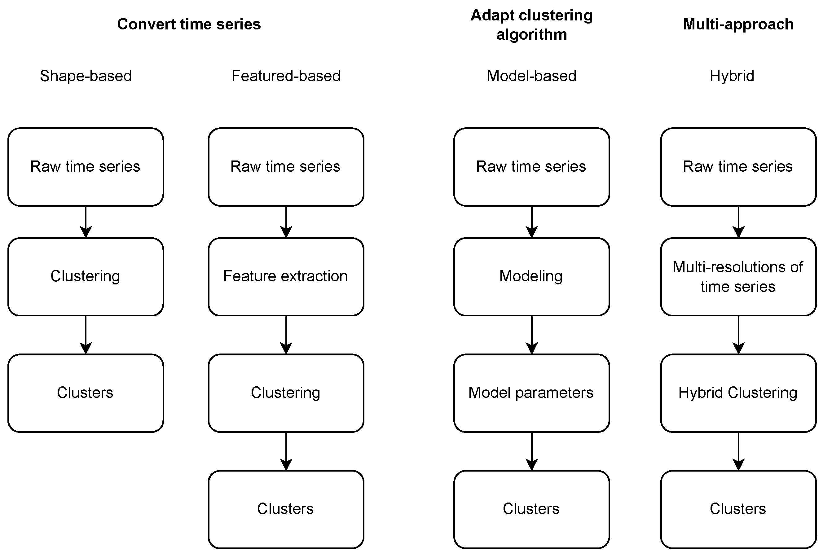
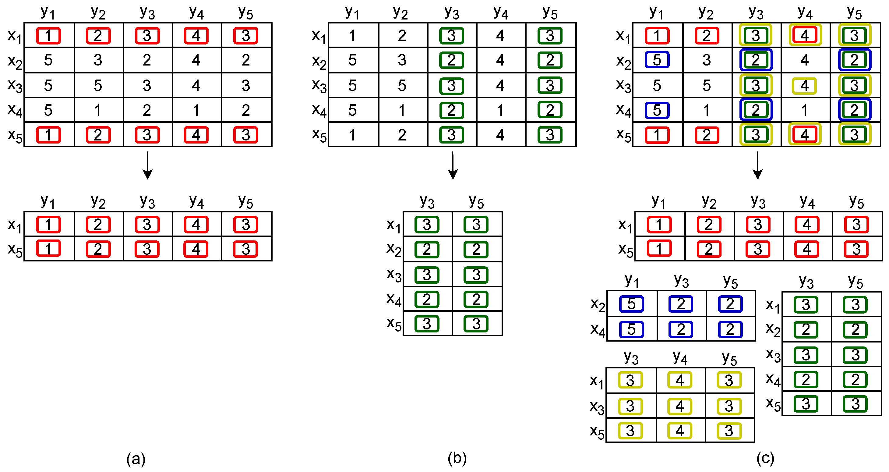
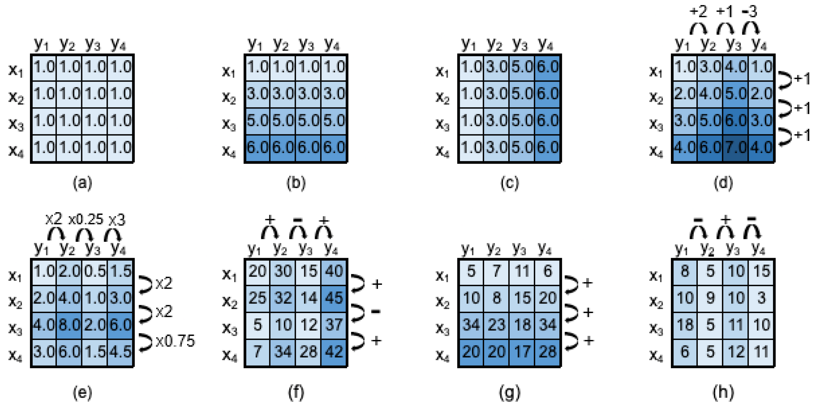
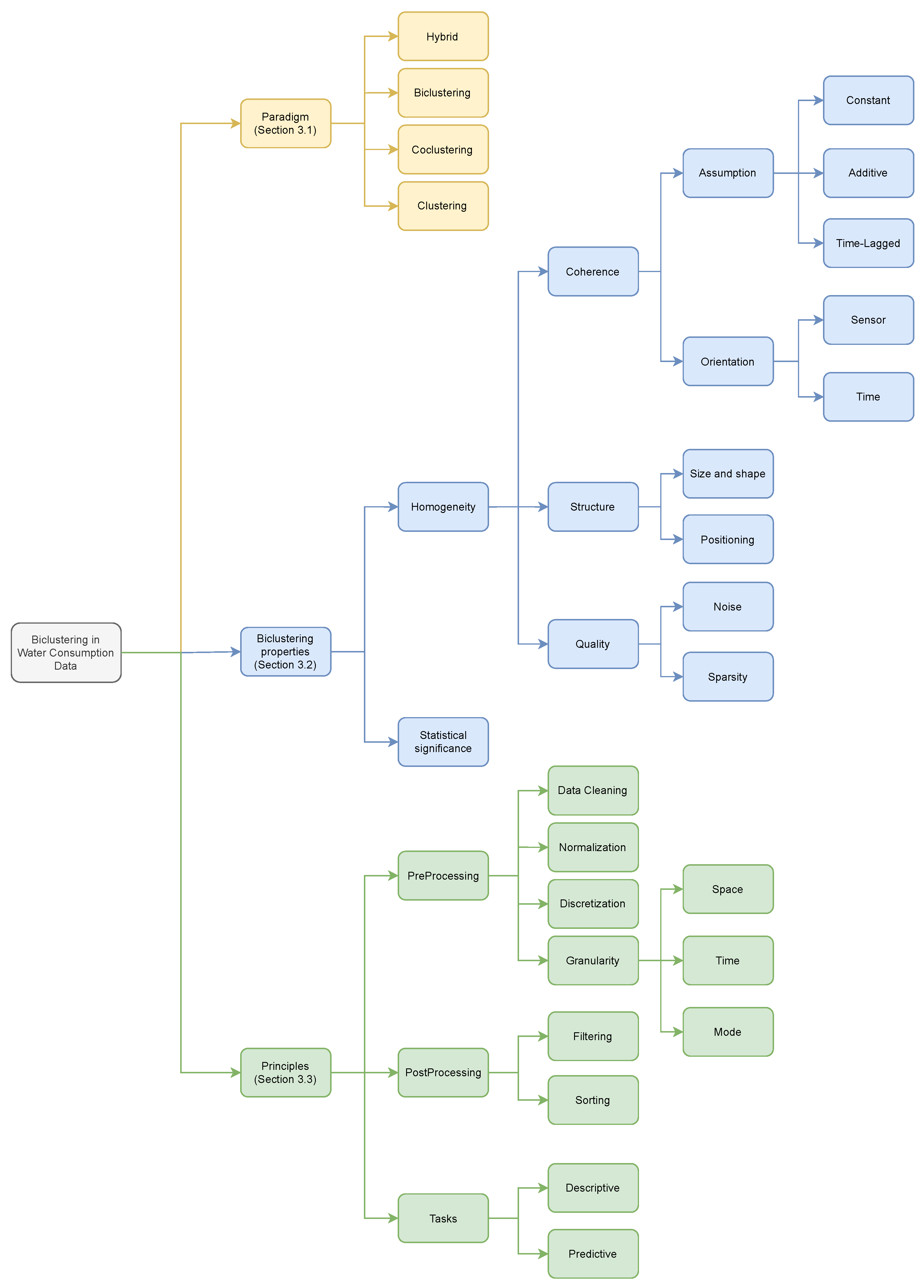
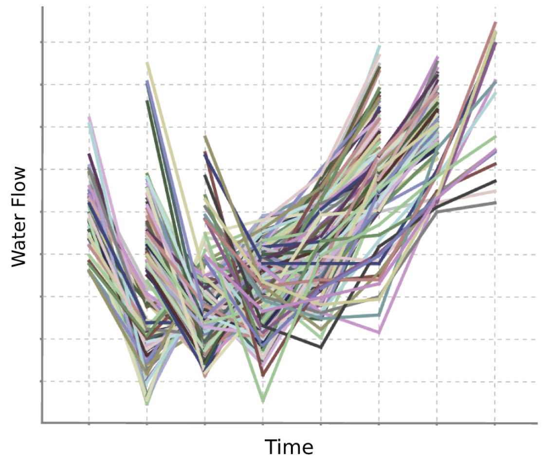
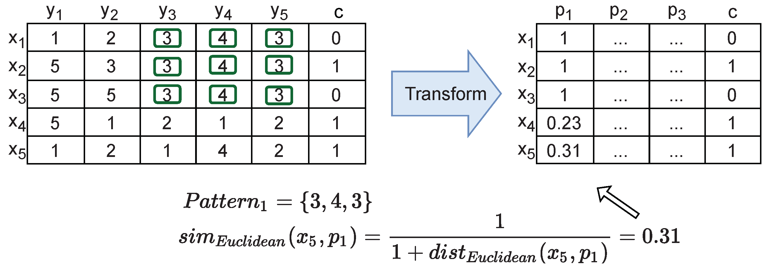
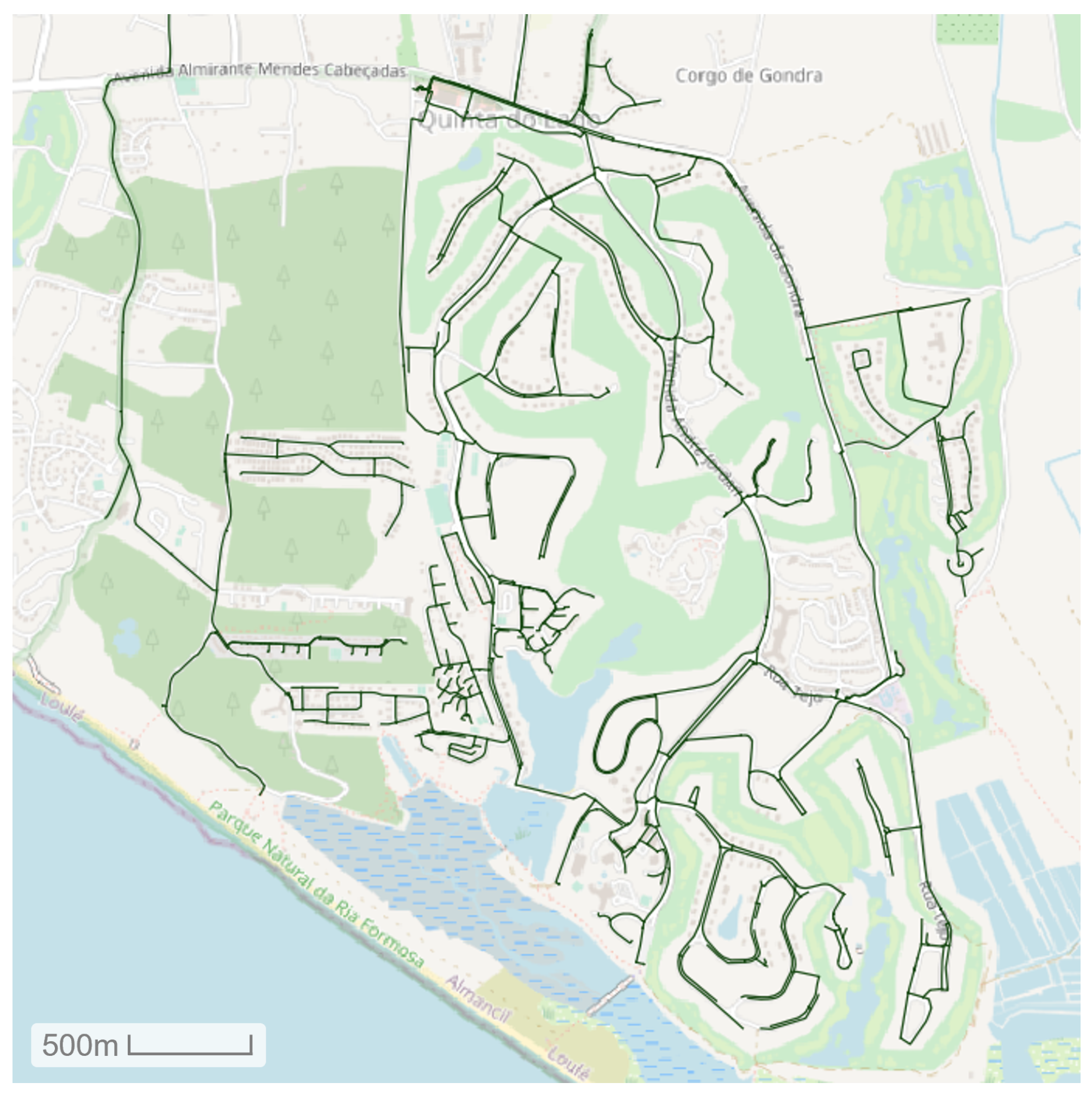
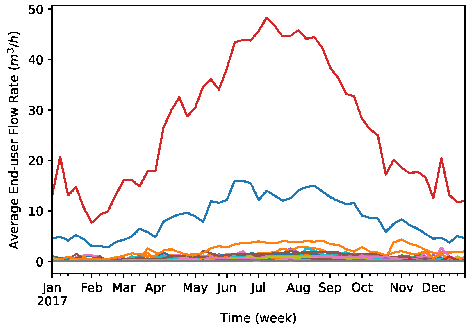
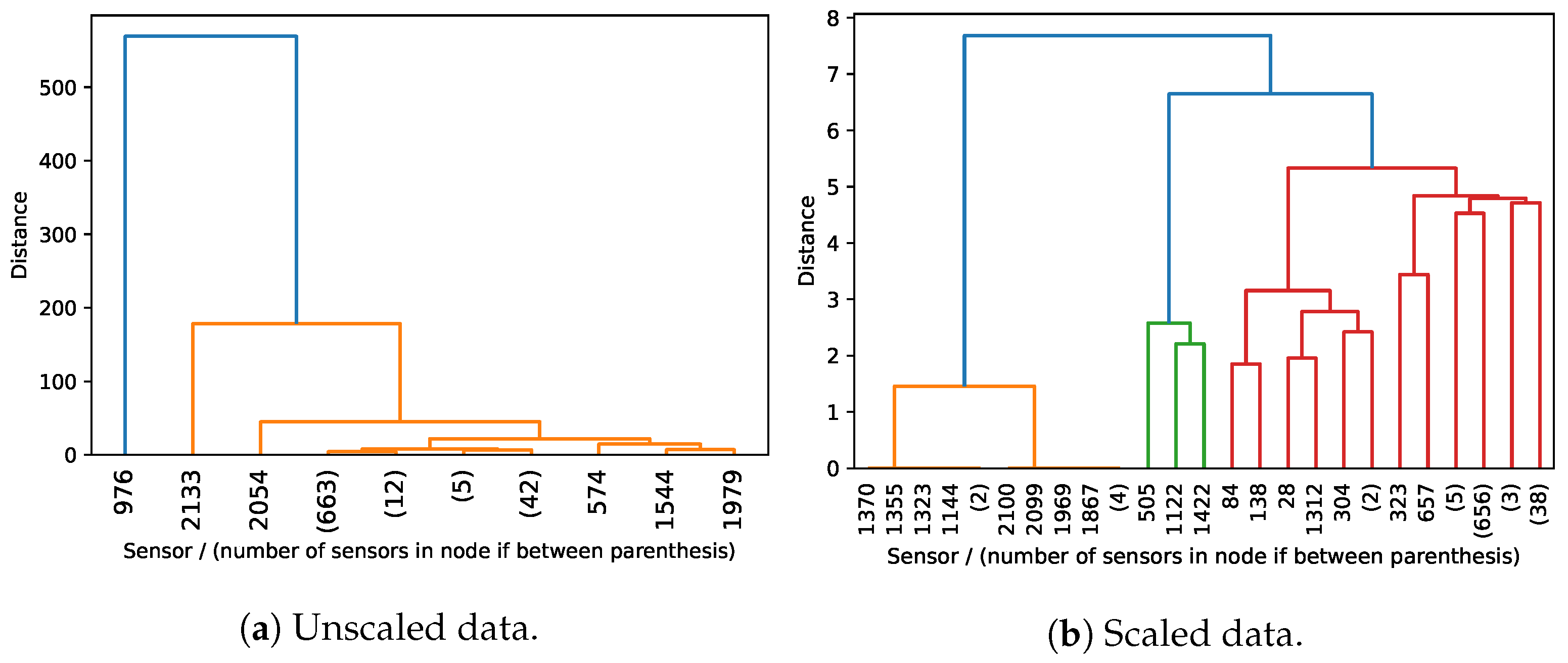
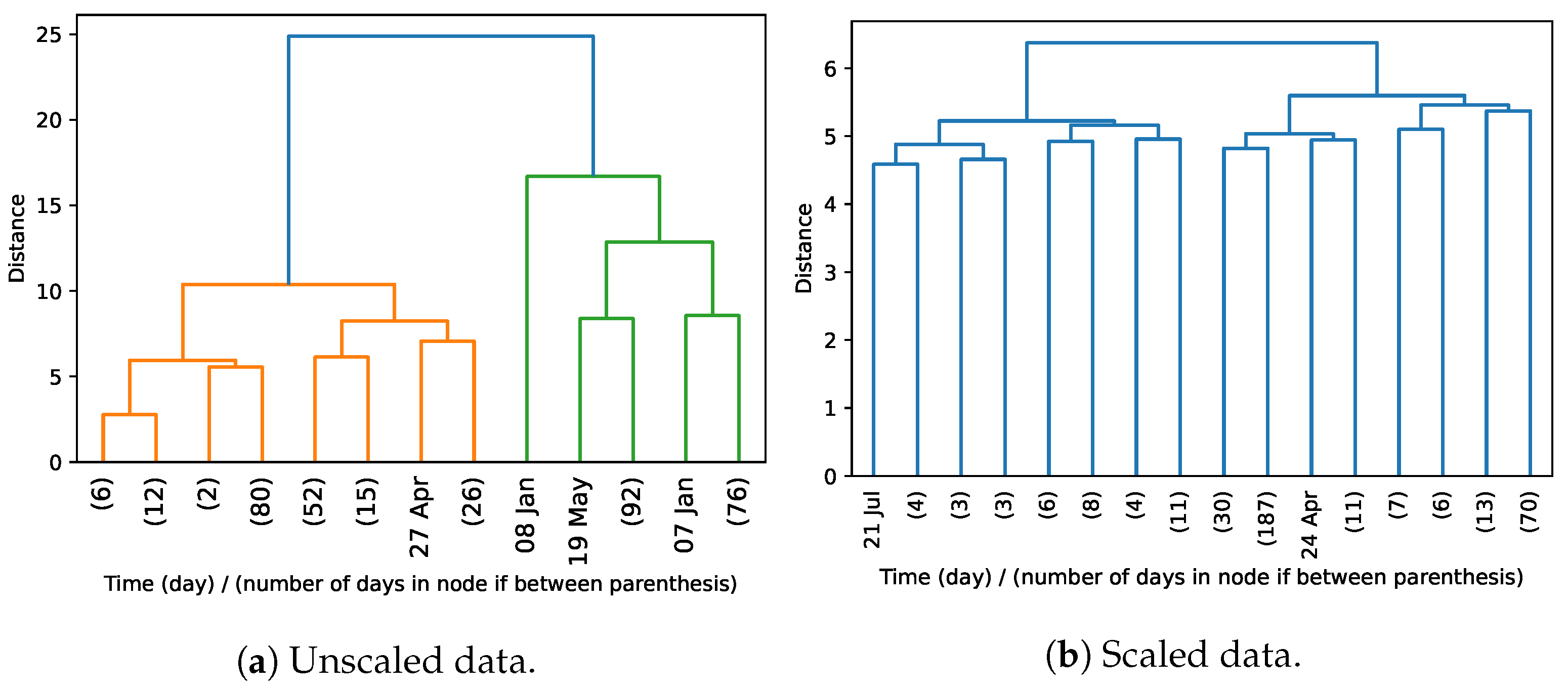
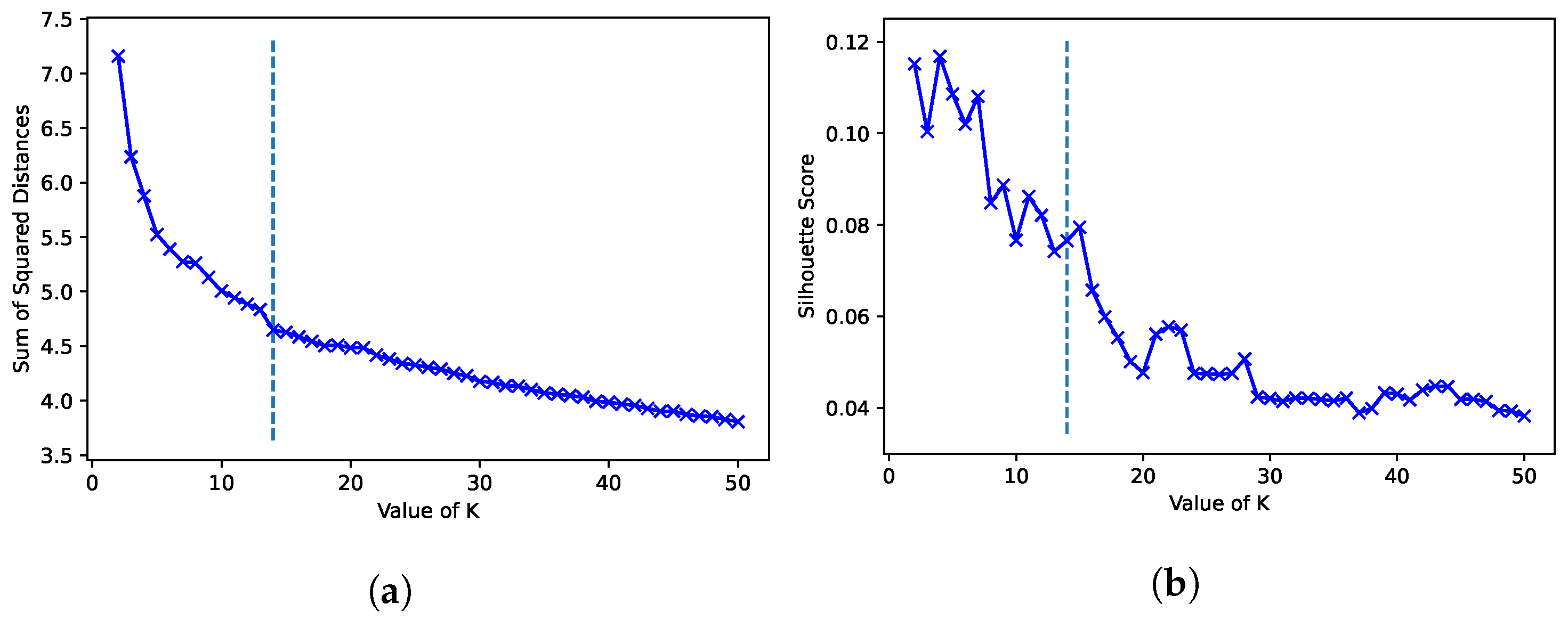
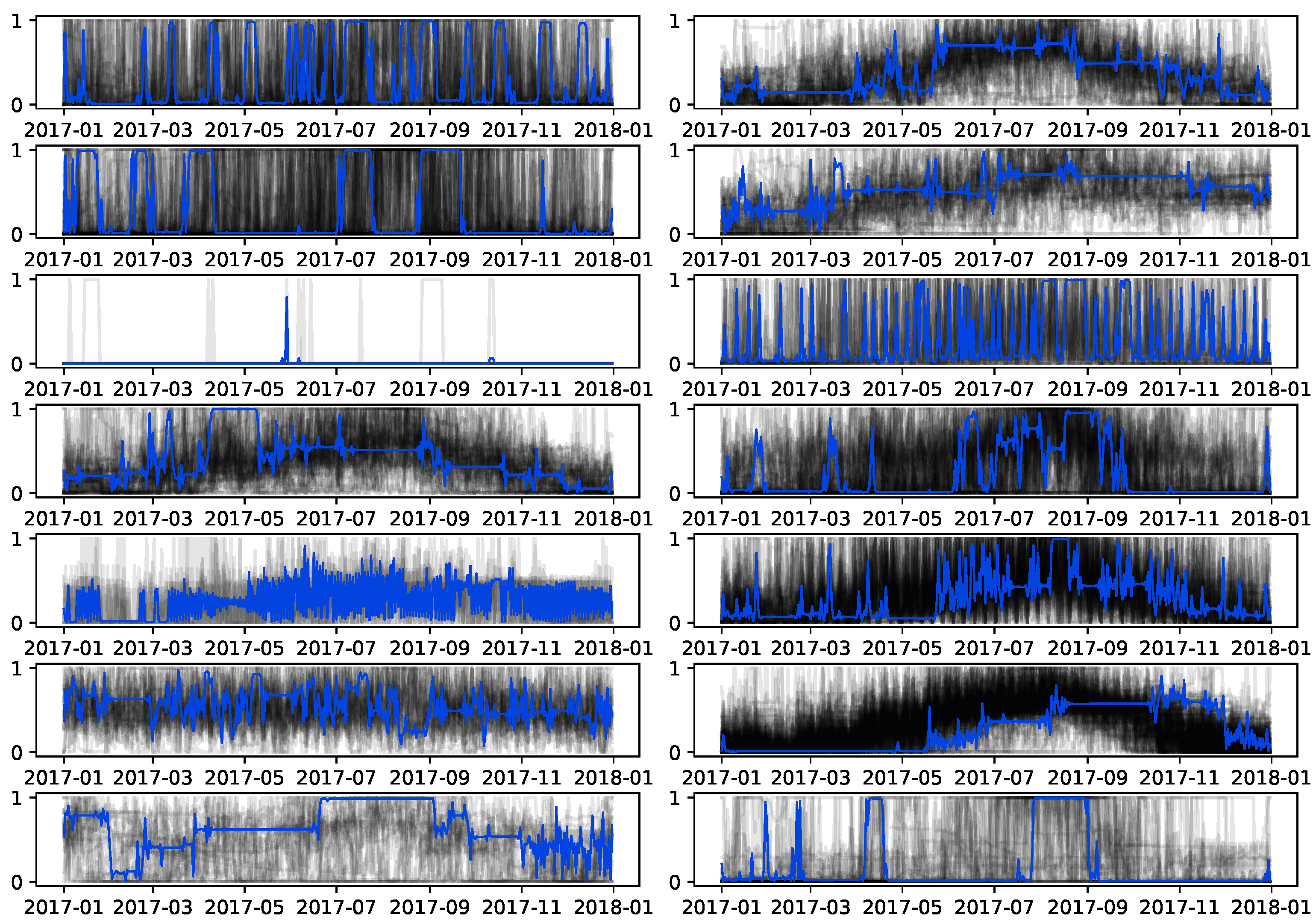
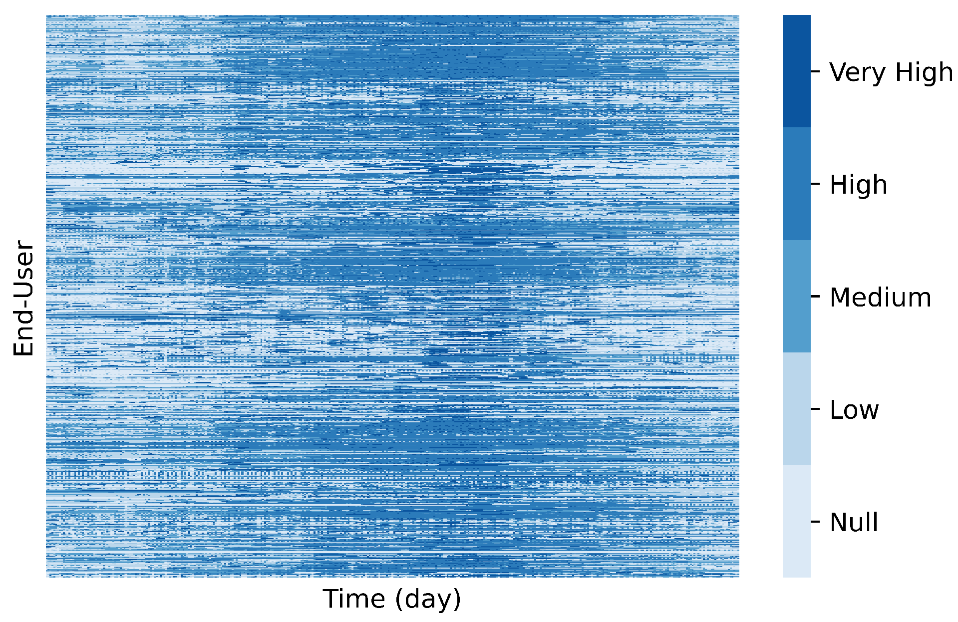
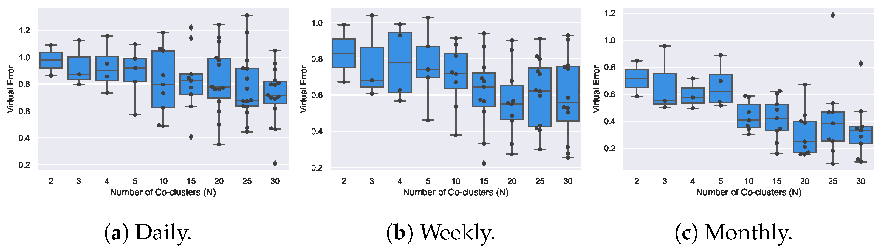
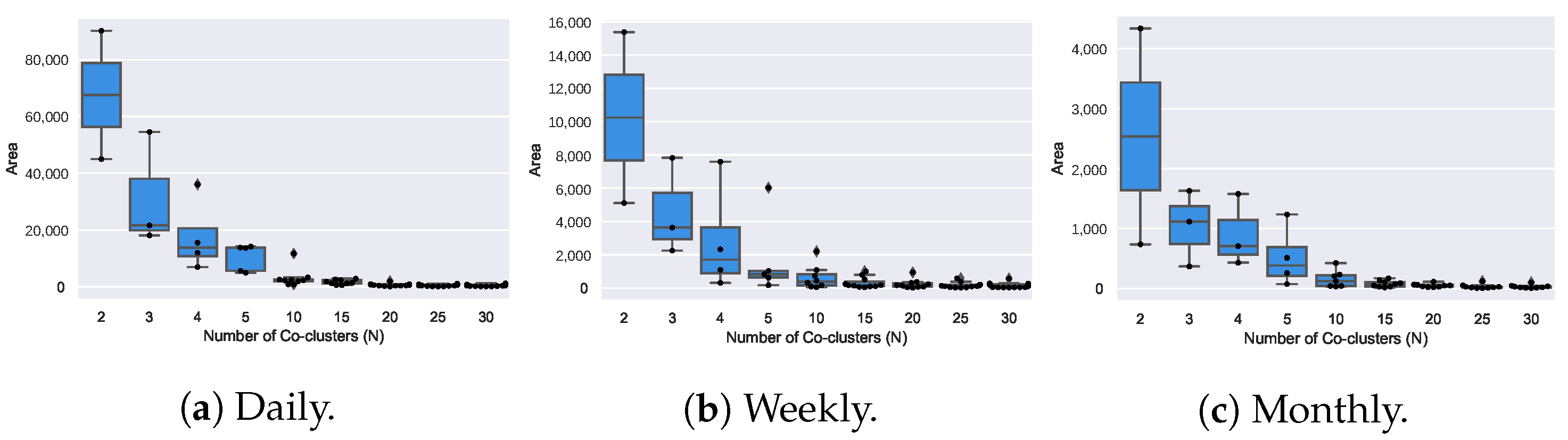
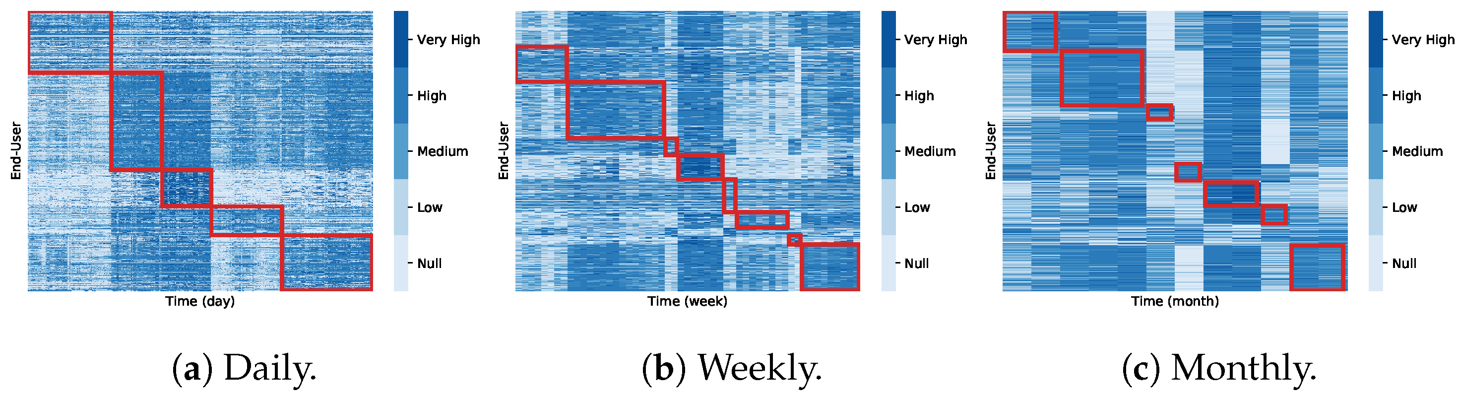
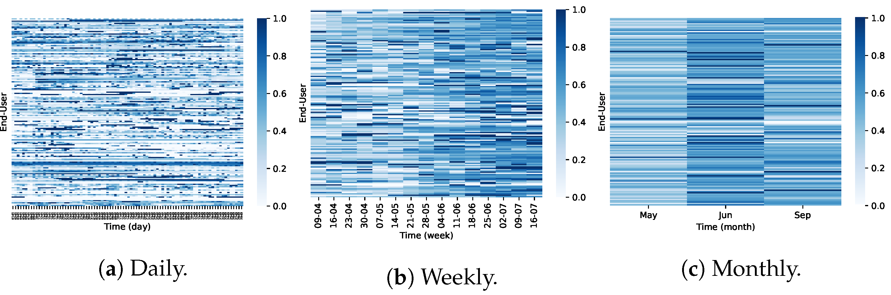
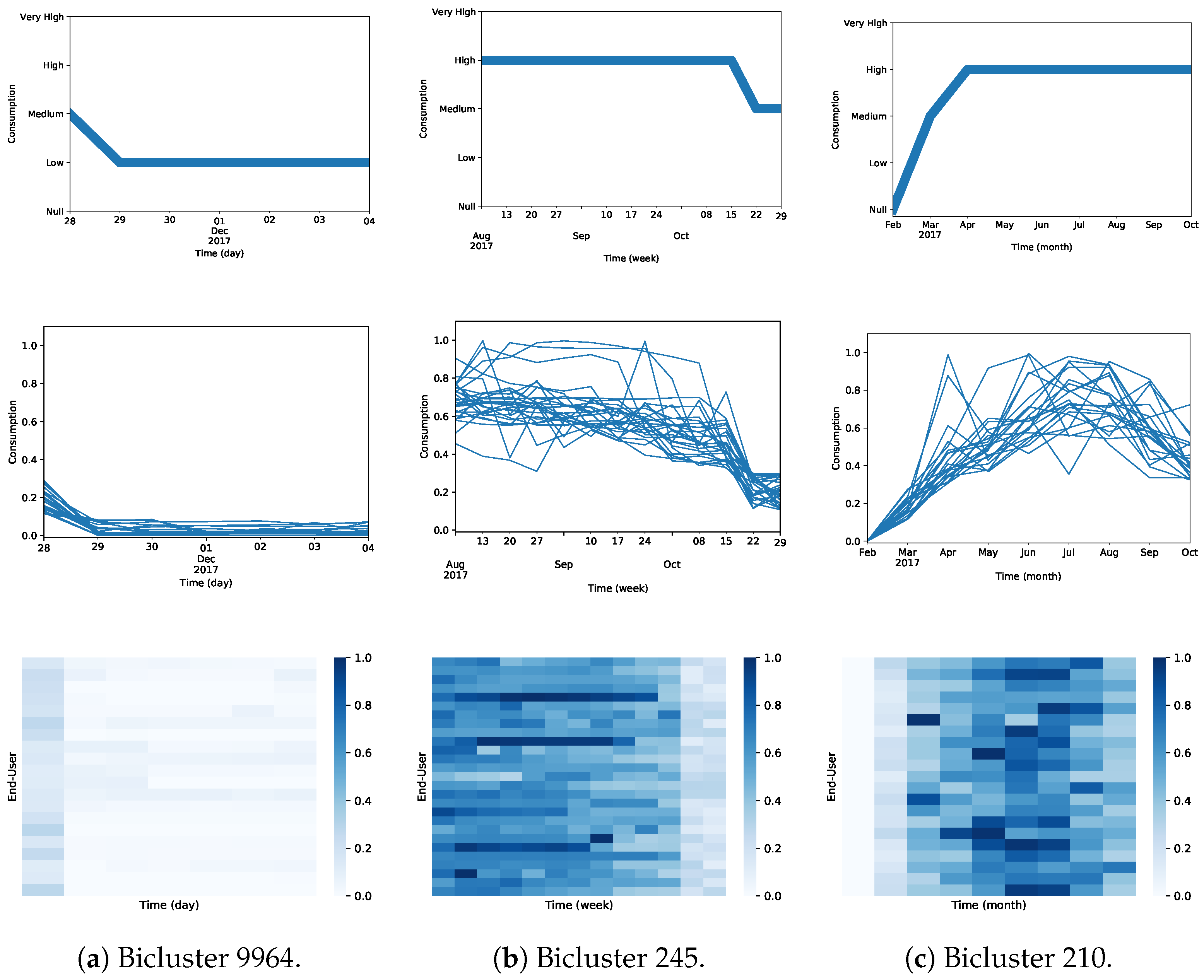
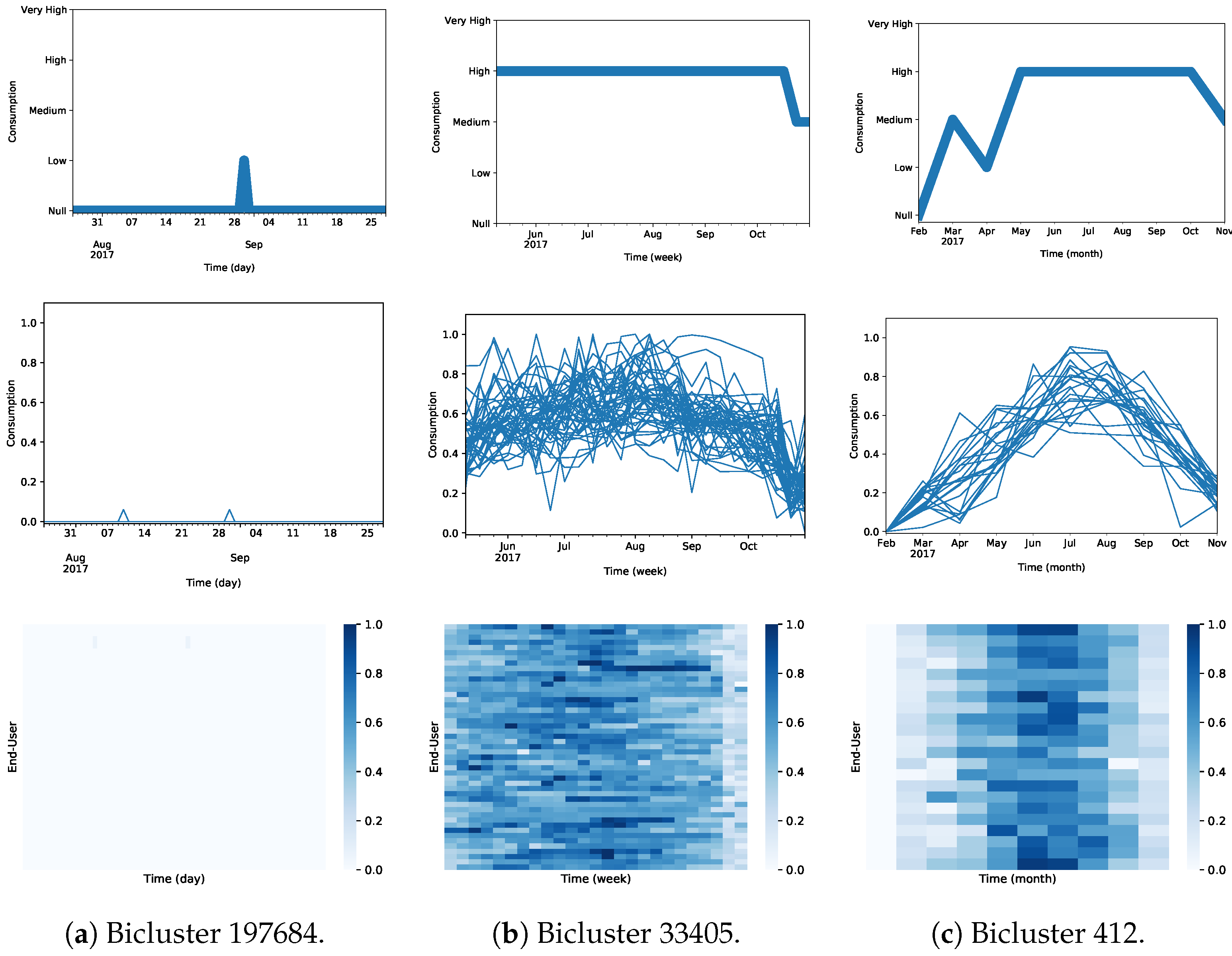
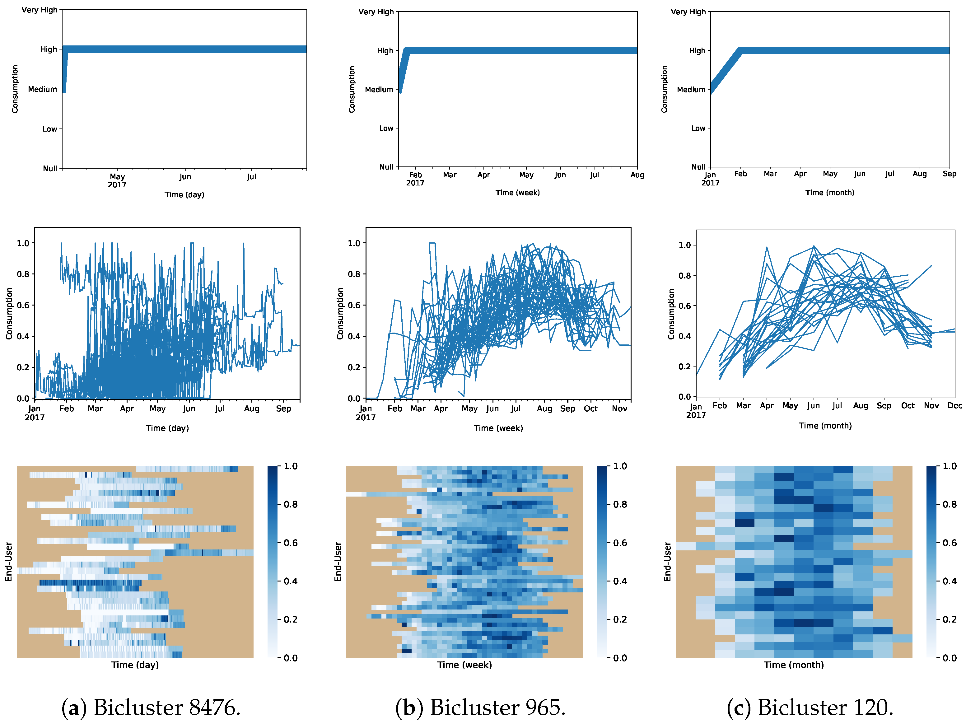
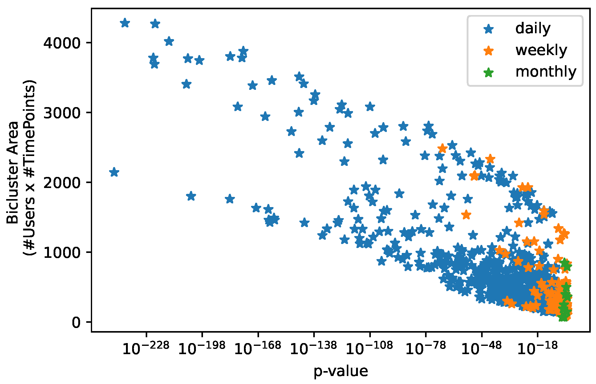
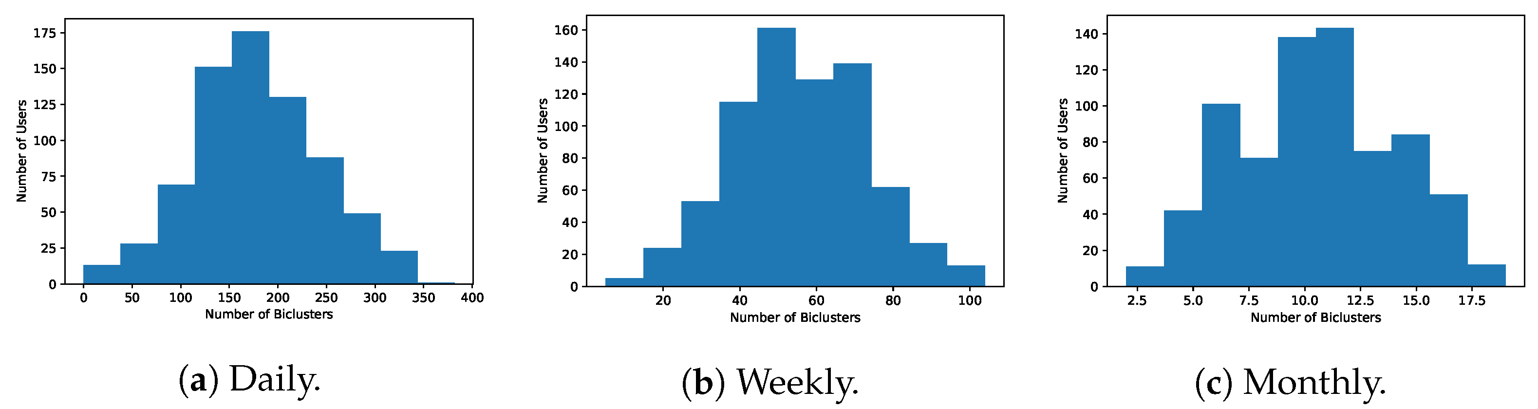
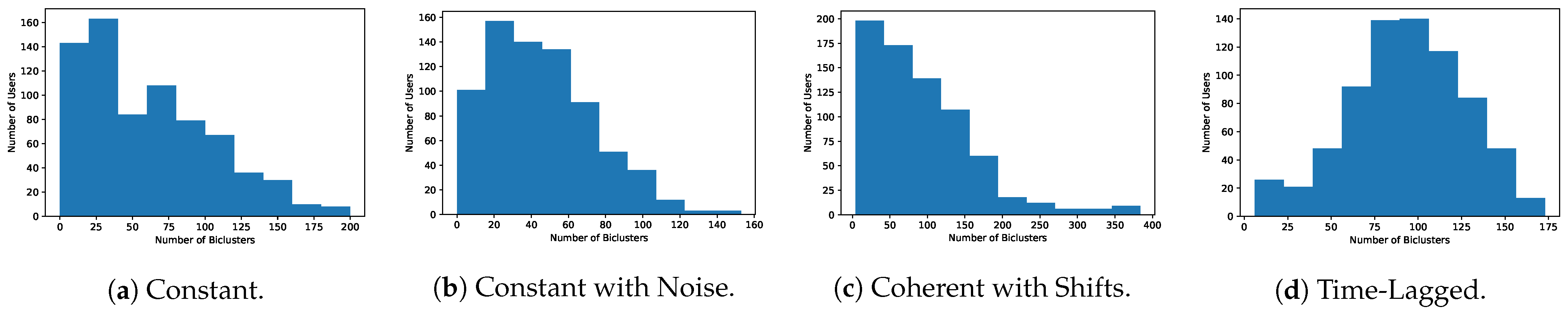
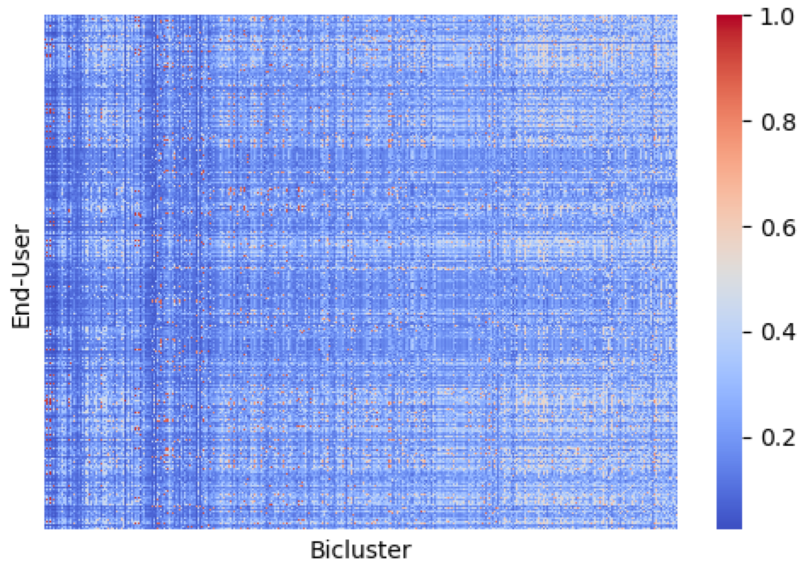
Table 1.
Selected coclusters for each of the scaled datasets at InfraQuinta, 2017.
| Dataset | ID | #Users | #Time Points (First, Last) |
|---|---|---|---|
| Daily | 0 | 161 | 88 (0, 87) |
| Weekly | 2 | 147 | 15 (14, 28) |
| Monthly | 1 | 142 | 3 (4, 8) |
Table 2.
Properties of the biclustering solutions found assuming constant patterns at InfraQuinta, 2017.
Table 2.
Properties of the biclustering solutions found assuming constant patterns at InfraQuinta, 2017.
| Solution | Post-Processed | ||||||
|---|---|---|---|---|---|---|---|
| Dataset | (min #Users, min #Time Points) | #bics | #bics | p-Value < 0.05 | p-Value < | ||
| Daily | (20, 7) | 18,666 | 65.2 ± 43.5 | 26.0 ± 20.7 | 655 | 655 | 655 |
| Weekly | (20, 4) | 1310 | 69.8 ± 65.9 | 9.4 ± 5.8 | 263 | 168 | 133 |
| Monthly | (20, 3) | 221 | 50.7 ± 51.5 | 4.5 ± 1.5 | 94 | 23 | 10 |
Table 3.
Constant biclusters picked for each of the datasets.
| Dataset | ID | #Users | #Time Points (First, Last) | p-Value |
|---|---|---|---|---|
| Daily | 9964 | 20 | 7 (331, 337) | 0.0029 |
| Weekly | 245 | 27 | 13 (31, 43) | 1.09 × 10 |
| Monthly | 210 | 21 | 9 (1, 9) | 5.17 × 10 |
Table 4.
Properties of e-CCC biclustering solutions with tolerance to noise under a constant pattern assumption at InfraQuinta, 2017.
Table 4.
Properties of e-CCC biclustering solutions with tolerance to noise under a constant pattern assumption at InfraQuinta, 2017.
| Solution | Post-Processed | ||||||
|---|---|---|---|---|---|---|---|
| Dataset | (min #Users, min #Time Points) | #bics | #bics | p-Value < 0.05 | p-Value 1 × 10 | ||
| Daily | (20, 7) | 786,232 | 72.3 ± 44.8 | 28.9 ± 21.7 | 2347 | 839 | 744 |
| Weekly | (20, 4) | 55,073 | 70.1 ± 63.3 | 11.7 ± 6.6 | 4304 | 279 | 160 |
| Monthly | (20, 3) | 6441 | 57.5 ± 59.8 | 5.6 ± 1.8 | 942 | 18 | 6 |
Table 5.
Constant biclusters tolerating noise picked for each of the temporal granularities.
| Dataset | ID | #Users | #Time Points (First, Last) | p-Value |
|---|---|---|---|---|
| Daily | 197,684 | 20 | 65 (206, 270) | 2.86 × 10 |
| Weekly | 33,405 | 47 | 25 (19, 43) | 1.83 × 10 |
| Monthly | 412 | 22 | 10 (1, 10) | 8.40 × 10 |
Table 6.
Properties of the biclustering solutions found assuming shifted factors at InfraQuinta, 2017.
Table 6.
Properties of the biclustering solutions found assuming shifted factors at InfraQuinta, 2017.
| Solution | Post-Processed | |||||||
|---|---|---|---|---|---|---|---|---|
| Dataset | (min #Users, min #Time Points) | L-Shift | #bics | #bics | p-Value < 0.05 | p-Value < 10 | ||
| Daily | (20, 7) | 1 | 38,933 | 87.0 ± 51.8 | 23.6 ± 16.4 | 625 | 593 | 588 |
| 2 | 46,308 | 111.4 ± 64.6 | 25.4 ± 17.1 | 383 | 340 | 330 | ||
| 3 | 32,669 | 124.6 ± 63.8 | 29.6 ± 21.9 | 367 | 332 | 323 | ||
| 4 | 16,033 | 114.8 ± 66.6 | 37.6 ± 26.5 | 345 | 310 | 301 | ||
| Weekly | (20, 4) | 1 | 2828 | 76.7 ± 74.0 | 8.2 ± 4.8 | 404 | 193 | 178 |
| 2 | 2743 | 96.2 ± 90.6 | 8.3 ± 5.0 | 369 | 153 | 131 | ||
| 3 | 1677 | 109.4 ± 97.5 | 10.0 ± 6.7 | 360 | 144 | 123 | ||
| 4 | 1391 | 84.5 ± 82.13 | 10.9 ± 7.0 | 357 | 141 | 121 | ||
| Monthly | (20, 3) | 1 | 372 | 56.3 ± 57.0 | 4.1 ± 1.4 | 113 | 33 | 21 |
| 2 | 318 | 65.2 ± 69.4 | 4.2 ± 1.4 | 108 | 27 | 18 | ||
| 3 | 251 | 60.3 ± 65.7 | 4.5 ± 1.5 | 108 | 30 | 21 | ||
| 4 | 245 | 55.4 ± 55.8 | 4.5 ± 1.6 | 108 | 30 | 21 | ||
Table 7.
Biclusters accommodating shifting factors (L = 4) picked for each of the datasets.
| Dataset | ID | #Users | #Time Points (First, Last) | p-Value |
|---|---|---|---|---|
| Daily | 141 | 23 | 8 (358, 364) | 0.002 |
| Weekly | 478 | 26 | 14 (30, 43) | 2.27 × 10 |
| Monthly | 239 | 21 | 9 (1, 9) | 5.17× 10 |
Table 8.
Properties of the biclustering solutions found assuming unbounded time lagged patterns at InfraQuinta, 2017.
Table 8.
Properties of the biclustering solutions found assuming unbounded time lagged patterns at InfraQuinta, 2017.
| Solution | Post-Processed | ||||||
|---|---|---|---|---|---|---|---|
| Dataset | (min #Users, min #TimePoints) | #bics | #bics | p-Value < 0.05 | p-Value < 10 | ||
| Daily | (20, 7) | 15,844 | 56.1 ± 51.3 | 26.5 ± 21.8 | 1471 | 1471 | 1471 |
| Weekly | (20, 4) | 1738 | 60.6 ± 61.9 | 10.2 ± 6.3 | 393 | 393 | 393 |
| Monthly | (20, 3) | 243 | 61.3 ± 66.2 | 4.8 ± 1.6 | 99 | 98 | 98 |
Table 9.
Time lagged biclusters picked for each of the datasets.
| Dataset | ID | #Users | #Time Points (First, Last) | p-Value |
|---|---|---|---|---|
| Daily | 8476 | 32 | 112 | 0 * |
| Weekly | 965 | 44 | 29 | 1.26× 10 |
| Monthly | 120 | 25 | 9 | 1.65 × 10⁻⁹ |
* The value is too small.
Publisher’s Note: MDPI stays neutral with regard to jurisdictional claims in published maps and institutional affiliations. |
© 2022 by the authors. Licensee MDPI, Basel, Switzerland. This article is an open access article distributed under the terms and conditions of the Creative Commons Attribution (CC BY) license (https://creativecommons.org/licenses/by/4.0/).
Share and Cite
MDPI and ACS Style
Silva, M.G.; Madeira, S.C.; Henriques, R. Water Consumption Pattern Analysis Using Biclustering: When, Why and How. Water 2022, 14, 1954. https://doi.org/10.3390/w14121954
AMA Style
Silva MG, Madeira SC, Henriques R. Water Consumption Pattern Analysis Using Biclustering: When, Why and How. Water. 2022; 14(12):1954. https://doi.org/10.3390/w14121954
Chicago/Turabian StyleSilva, Miguel G., Sara C. Madeira, and Rui Henriques. 2022. "Water Consumption Pattern Analysis Using Biclustering: When, Why and How" Water 14, no. 12: 1954. https://doi.org/10.3390/w14121954
Note that from the first issue of 2016, this journal uses article numbers instead of page numbers. See further details here.