
Analyzing and Assessing Dynamic Behavior of a Physical Supply and Demand System for Sustainable Water Management under a Semi-Arid Environment

1
College of Agricultural, Consumer and Environmental Sciences, New Mexico State University, Las Cruces, NM 88003-8003, USA
2
New Mexico Water Resources Research Institute, New Mexico State University, Las Cruces, NM 88003-8001, USA
*
Author to whom correspondence should be addressed.
Water 2022, 14(12), 1939; https://doi.org/10.3390/w14121939
Submission received: 26 April 2022
/
Revised: 9 June 2022
/
Accepted: 9 June 2022
/
Published: 16 June 2022
(This article belongs to the Special Issue Integrated Water Resources Management (IWRM), a Holistic Approach to Sustainable Water Management)
Abstract
:The extensive interest in sustainable water management reflects the extent to which the global water landscape has changed in the past twenty years, which is a natural development of changes in water resources and an increase in the level of imbalance between water supply and demand. In this paper, a simulation model based on system dynamics (SD) methodology was developed to aid sustainable water management efforts in a semi-arid region. Six policy scenarios were used to study, analyze, and assess water management trends in the Southeast region of New Mexico, USA. The modeling process included two phases: calibration (2000–2015) and future prediction (2016–2050). Several statistical criteria were applied to assess the developed model performance. The findings revealed that the simulated outputs were in excellent agreement with the historical data, indicating accurate model simulation. The SD model’s determination coefficients ranged from 0.9288 to 0.9936 and the index of agreement values ranged from 0.9397 to 0.9958. Findings for the business-as-usual scenario indicated that total water withdrawals and total population will continue to rise, whereas groundwater storage, agricultural consumptive water use, and total consumptive water use will decrease over the simulated period. Sensitivity analysis using Monte Carlo simulation indicated that cultivated irrigated land change is the most influential parameter affecting groundwater storage, water supply storage change (total withdrawals), agricultural consumptive water use, and total consumptive water use. The changes occurring in the agricultural cultivated area had a great influence on controlling the groundwater system. Overall, the results showed that our SD model has been successful in capturing the system’s dynamic behavior, and confirmed its capability in modeling water management issues for policy and decision makers under semi-arid conditions.
1. Introduction
The complexity of hydrological, environmental, agricultural and social parameters and factors, and the diversity of opinions and concerns related to water use for varied purposes are now increasingly demanding water management in a more efficient and comprehensive way. Water is a vital natural resource that people, animals, and plants require for life, growth, and development. It is the main component of our ecosystem and pivotal for maintaining civilization, progress, and human prosperity. Moreover, water is considered an economic good classified as a necessity [1]. The sustainable management of water resources is necessary for supporting social, economic, ecological, and environmental development [2,3,4]. With the rapid population growth, urbanization, industrialization, and climate change, problems relating to water and hydrological resources management have become more visible [5,6]. Effective water demand–water supply management is the backbone of any sustainable development for hydrological, economic, and environmental systems, especially in arid regions [7,8,9].
Water management is more difficult in semi-arid and arid regions that rely greatly on groundwater [10]. In general, groundwater is the primary water source, particularly in zones and areas with surface water is lacking, where it plays a vital role in suppling water in semi-arid and arid regions. For example, the Ogallala aquifer is the biggest groundwater source in the United States (US) that underlies portions of eight states including: New Mexico, Texas, Wyoming, Colorado, Kansas, Oklahoma, South Dakota, and Nebraska. It is the main source of crop water irrigation requirements, and around 30% of the groundwater applied for irrigation throughout the US is pumped from the Ogallala aquifer [11,12]. However, this could result in groundwater depletion, reduced well productivities, yields and qualities, increased pumping costs, and ecosystem harm [13,14]. Therefore, managing water in general and groundwater in particular in semi-arid and arid regions should use the best and most successful methods and techniques to develop solutions, simulations, plans, strategies, and policies for sustainable management.
Many techniques and methods have been successfully suggested and applied to deal with the complexity related to different influencing elements, parameters, feedbacks, and systems in water management, and one of the most important of them is the system dynamics (SD) [15,16,17,18,19,20,21,22,23,24,25,26,27,28,29,30,31,32,33,34,35,36,37]. System dynamics (SD) are simulation processes to help explain interactions between different parameters and sub-systems, which influence the overall system’s dynamic behavior. Basically, using SD modeling can facilitate investigating water management by conceptualizing non-linear causal connections and feedback loops within specific borders between linked systems [15,16,17,18]. Water management based on SD methodology helps to consider the most sensitive factors and variables in order to increase water usage performance on the system scale [19,20]. The weakness of traditional mathematical modeling approaches can be removed by system dynamic simulation. However, traditional modeling and statistical methods such as classical regression, critical path method, work breakdown structures, or program evaluation and review technique ignore interactions, feedback, and interrelationships among different multi-parameters and variables [21,22,23], which means that water management behavior will be difficult to be comprehensively and systematically investigated. This is because water management, in order to be successful and sustainable, must take into account feedback, reactions, and overlapping interrelations between water systems and other parameters and systems that have a connection with it, whether they be economic, social, agricultural, ecological, or environmental.
Generally, SD models for a broad range of water and hydrological applications have been utilized. They have been applied to manage surface water [24,25], assess water quality [26,27], plan water resources [28], manage drought [29], analyze irrigation efficiency [30], model crop water demand [7], control flood [31], simulate water supply aquifer [32], model water-reallocation [33], analyze water conflict [34], simulate groundwater governance [35], and evaluate water resources carrying capacity [36]. A comprehensive and up-to-date review of studies and investigations employed and applied SD approaches in water and hydrological sector can be found in [37]. However, the knowledge of SD for simulating and modeling water management comprehensively and sustainably in a semi-arid or arid environment is limited. Overall, SD methodology can be effectively applied to describe, analyze, and assess important water system variables/parameters that have interesting dynamic behavior for sustainable water management. Thus, to achieve sustainable water management and understand the water demand pressure on available water resources and, especially, groundwater, this study uses system dynamics (SD) methodology and modeling to simulate, analyze, and evaluate the present conditions and future trends of a water system in a semi-arid region. Therefore, the specific objectives of our investigation are to (1) develop an SD model to simulate water management in southeast New Mexico, USA; (2) evaluate the effectiveness of the SD model using a statistical comparison among the outputs produced from the model and historical data; (3) perform a sensitivity analysis using Monte Carlo simulation for evaluating the impacts of some parameters on the developed model; and (4) discuss and compare several policy scenarios to help with sustainable water management decision-making processes. Moreover, it is hypothesized that SD modeling would provide valuable results and information about the dynamic behavior of water systems in a semi-arid environment. Specifically, it is hypothesized that some of the most important dynamical hydrological influences in the SE-NM region’s water system would be demonstrated, such as increased total water supply storage change (total withdrawals), groundwater storage decline, and decreased cultivated area impacts on agricultural consumptive water use and total consumptive water use.
2. Materials and Methods
2.1. Study Area Description
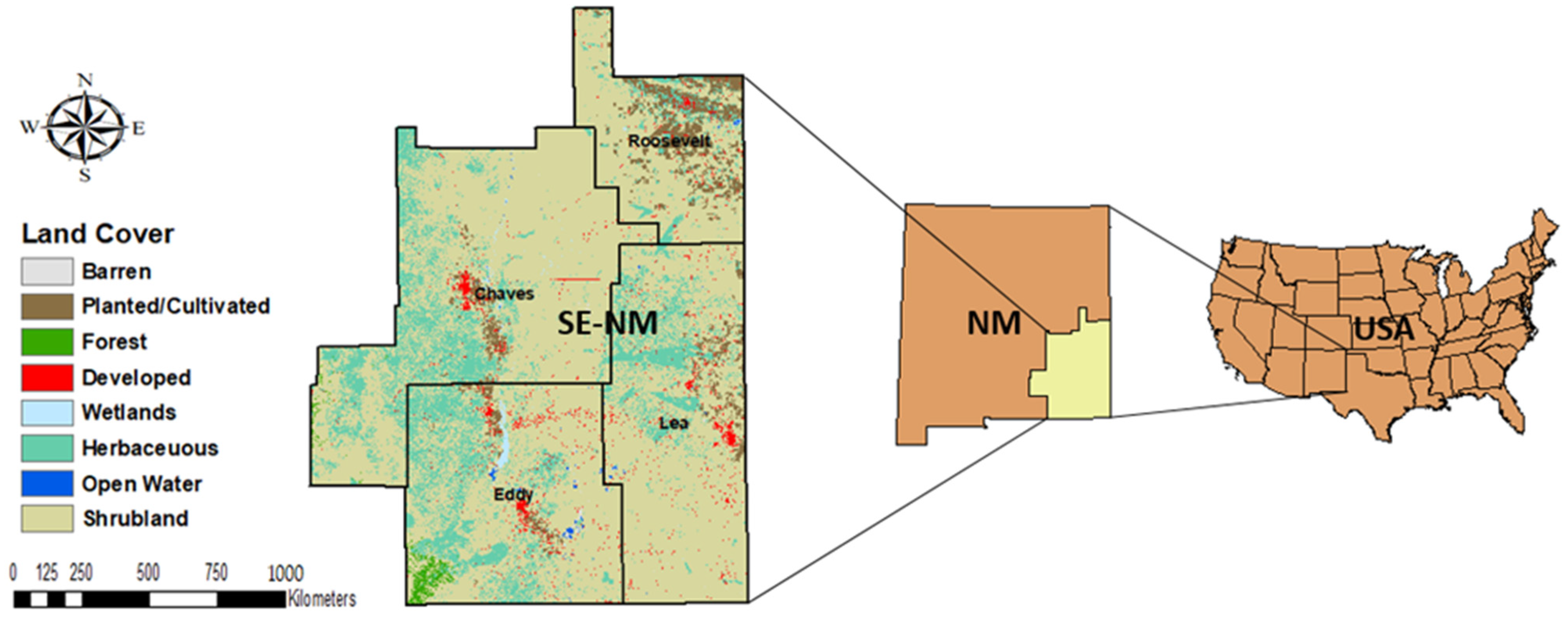
The southeast New Mexico (SE-NM) region is centered at latitude 33°23′1.64″ N and longitude 103°46′33.31″ W. It lies within the administrative boundaries of four counties: Eddy, Lea, Roosevelt, and Chavez (Figure 1). The whole area of SE-NM region is 44,276 km2, which accounts for around 14% of New Mexico’s land area. The 2010 U.S. Census estimated the population of SE-NM to be 204,047 [38].
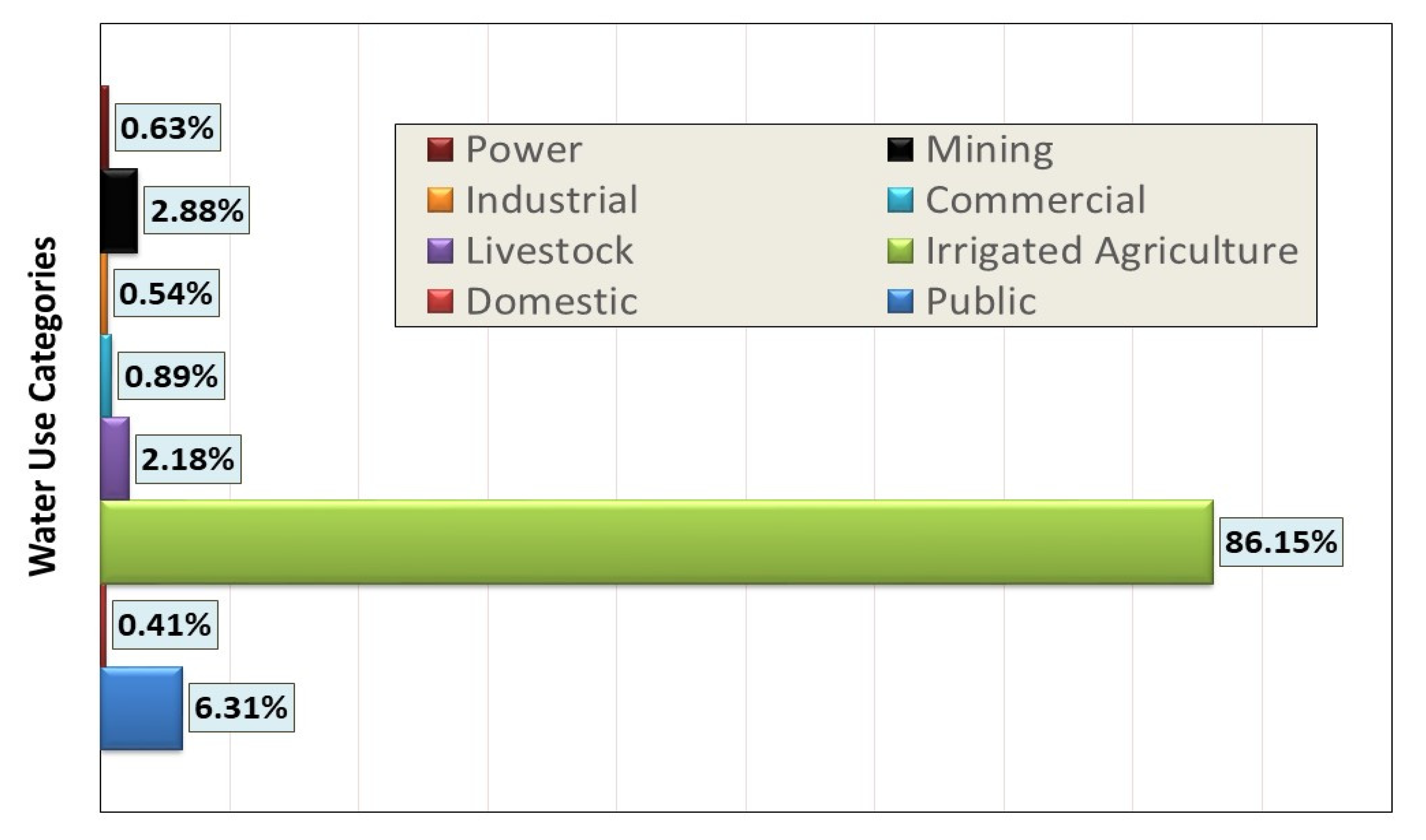
Due to its semi-arid climate, the precipitation of the SE-NM region occurs during monsoon months spanning June, July, and August. Historically, the average annual temperature range is from 23.91 °C to 6.99 °C, whereas the average annual precipitation is about 372.74 mm [39]. The dominant land cover is shrubs throughout the region, whereas the surface open water is very limited, as shown in Figure 1. Thus, water withdrawal sources for SE-NM are almost exclusively groundwater, accounting for around 83% of the region’s total water withdrawals [40]. There are eight main water use categories in SE-NM: public, domestic, irrigated agriculture, livestock, commercial, industrial, mining, and power (Figure 2). Consequently, according to the New Mexico Office of the State Engineer (OSE), water use by category in 2011–2015 was: 6.31% public, 0.41% domestic, 86.15% irrigated agriculture, 2.18% livestock, 0.89% commercial, 0.54% industrial, 2.88% mining, and 0.63% power [40]. Thus, about 90% of SE-NM region’s water is used for agriculture (irrigated agriculture and livestock). Therefore, there is a need for innovative solutions and approaches and policies for sustainable agricultural water management, taking into consideration the local water conditions in this region and the demand and supply, and the balance between them.
2.2. System Dynamics Modeling Theory
In the 1950s, J.W. Forrester presented System Dynamics (SD) in order to examine complicated business problems, such as management of manufacturing processes and stocks [16]. A mathematical modeling framework supported by feedback control theory characterizes and describes the close interactions and connections between different parameters [15,16,17]. SD has many advantages especially with systems with high levels of multi- and non-linear parameters and relationships [15,16,17]. SD is a modeling framework using systems theory and has been used to various fields to comprehend the dynamic behaviors of various complex systems. The SD modeling process typically involves the following phases: problem definition, conceptualization, formulation, model assessment, scenario analysis, and policy implementation [15,37,41]. Thus, system elements and their common relations should be predetermined. Table 1 depicts fundamental components found in all SD models and explains each element of the system according to Vensim syntax [42].
Overall, SD modeling is based on causal mathematical models founded on the underlying principle that the structure of a system causes measurable and predictable behavior [15]. SD modeling begins with determining the system’s structure to identify the interactions and relationships between various system components [15,29,37]. These relationships are both qualitative (causal loop diagram) and quantitative (stock and flow diagram) and are accompanied by mathematical formulations [29,30]. There are many software options for implementing this, such as Stella (isee systems, Lebanon, NH, USA), Powersim (Powersim Software AS, Bergen, Norway), and Vensim (Ventana Systems Inc., Harvard, MA, USA), but the most commonly used software in water research is Vensim [37]. The following formulas indicate the fundamental mathematical expressions that Vensim uses [42].
The g, h, and f are arbitrary nonlinear functions, which may change throughout time. Equation (1) refers to the system evolution throughout time period. Equation (2) is the same as Equation (1) but in differential form, whereas Equation (1) is in integral form. The syntax used by Vensim DSS to represent equations corresponds more closely to Equation (1). Equation (3) expresses rates calculation. Equation (4) refers to the intermediate results to calculate the rates. Equation (5) expresses the system initialization [42].
2.3. System Dynamics Model Development
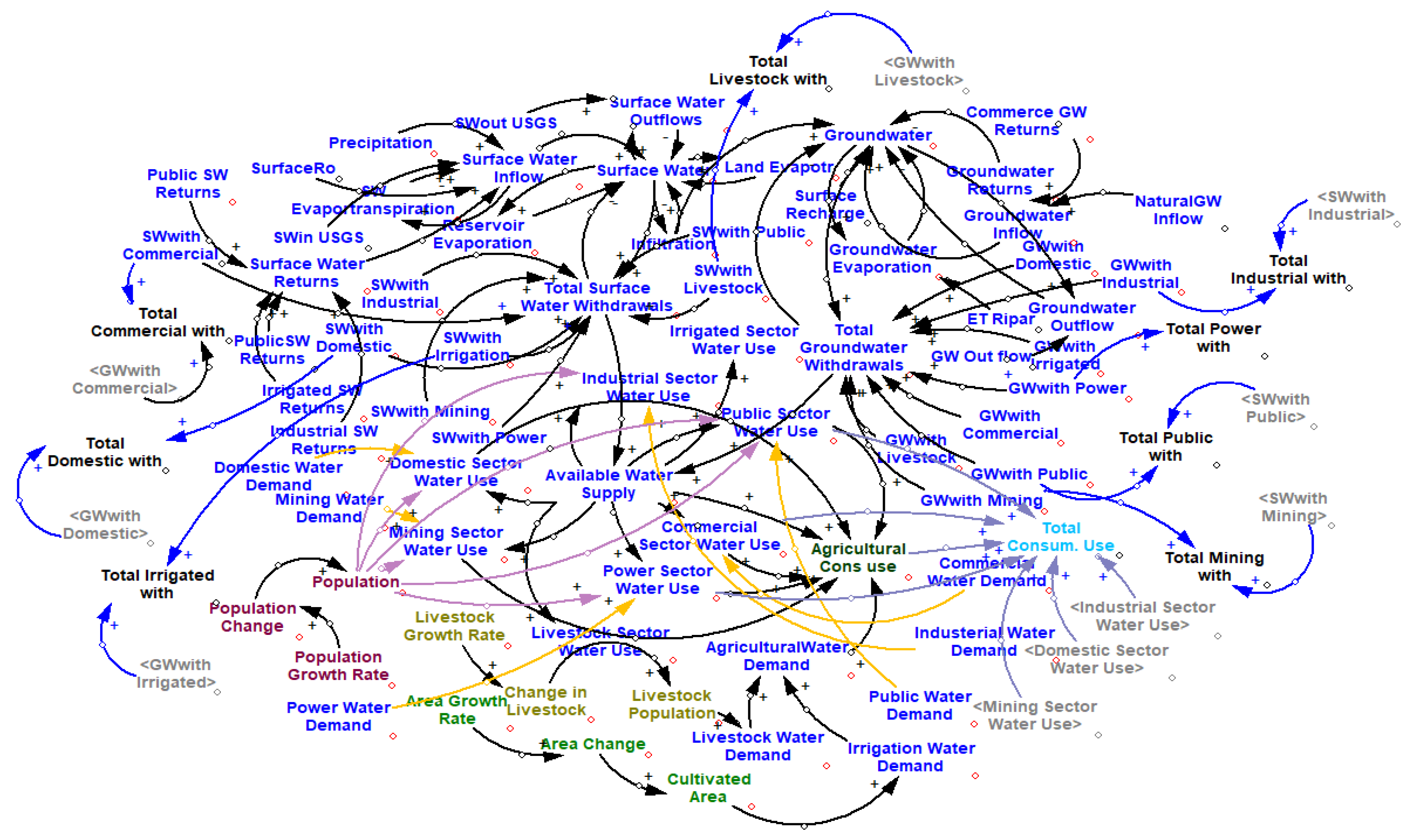
This section provides the steps that were used to develop our SD model. The main and first step in developing our SE-NM model included creating a casual loop diagram (CLD) for modeling used parameters to offer a foundation for a stock and flow diagram (SFD) [29,30,37]. A more complete explanation of the SD models development is provided by the authors in [37]. Figure 3 displays the CLD of SE-NM, whereas Figure 4 illustrates the SFD for studying and simulating water management in the SE-NM region. This CLD provides valuable information about whole system and its elements, causal relationships among them, and feedbacks loops [19,20], as demonstrated in Figure 3.
A CLD is made up of four main components: the parameters, their links, and the links’ and feedbacks’ signs. Hence, we initially identified the parameters or variables that are essential to the water system. In our case, the water supply system involves both groundwater and surface water. Of note, over 80% of total water use in the SE-NM region is from groundwater [40]. In spite of that, the surface water was included in the model to give a realistic picture of the water system in that region and to obtain reliable results from the model. To avoid mathematically non-absorbable extreme phenomena, such as extreme precipitation [43], pertinent dynamic quantities are assumed to be at least sectionally smooth. In SE-NM, the water demand sector includes domestic, industrial, mining, public, power, irrigation, commercial, and livestock water demands. However, the water system, especially the water demand, is influenced by total population, livestock population, and total cultivated area, and hence they must be considered in our model. Therefore, the SE-NM water system or SD model was divided into five major sectors or subsystems, including total population, cultivated area, livestock population, water supply, and water demand for different sections and uses. The SE-NM model’s subsystems, parameters, variables, and their types are explained in Appendix A. The feedback relationships are developed to represent the effect of different parameters, sectors, or subsystems on each, in which the “+” sign indicates a growth or rise in the parameter at the arrow’s top, and the “-” sign indicates a decline in that parameter, as demonstrated in Figure 3.
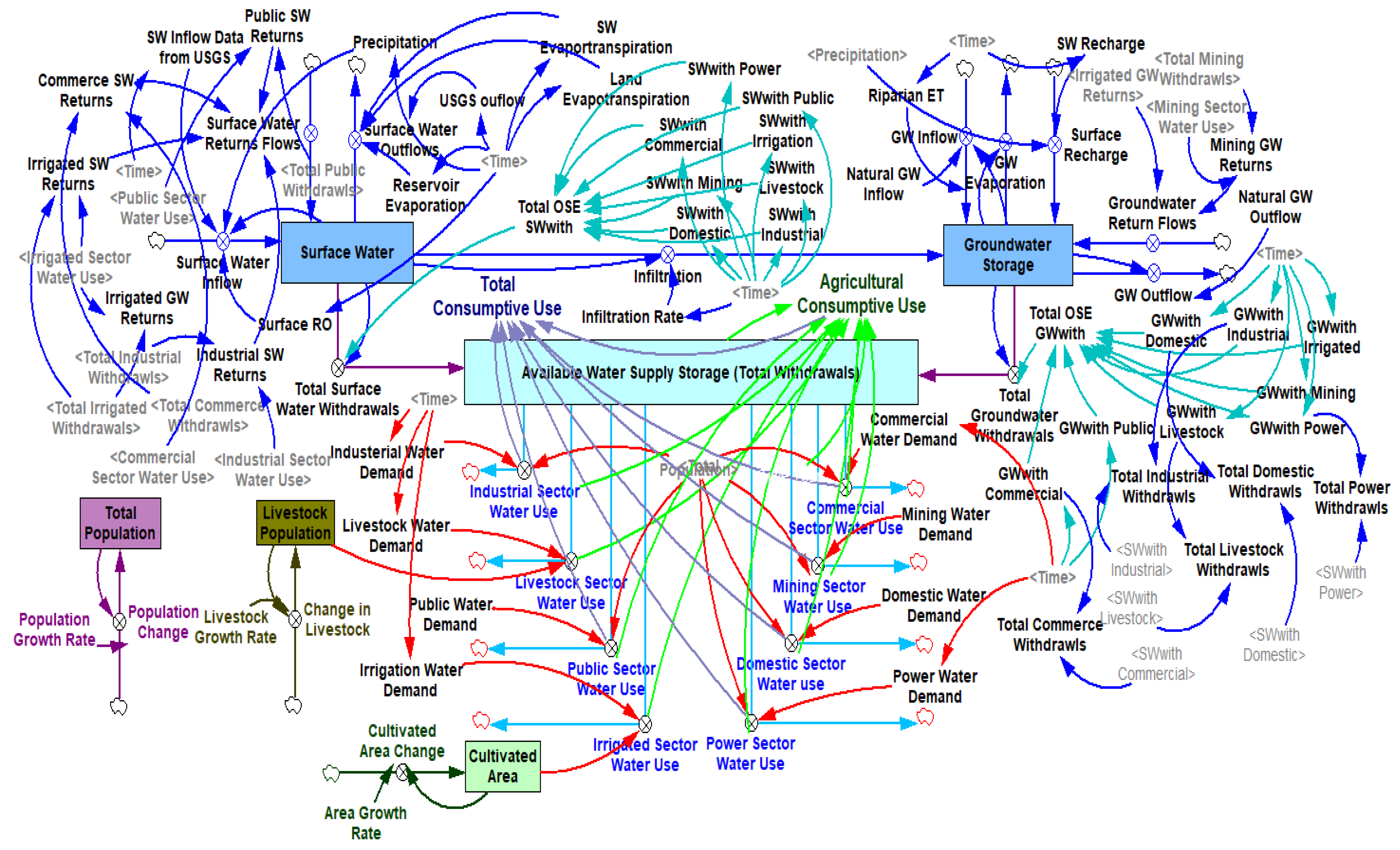
The second step in SD model development is creating the SFD (Figure 4) based on the established CLD. The SFD defines the relationships among parameters using mathematical formulas and input data, and expresses the system as stocks and flows. Stocks (levels) are computed, representing any parameter which through time accumulates, whereas flows are computed through a time period showing parameters which affect stocks [24,25,44]. With a time phase or step of one year, our total simulation interval is from 2000 to 2050. The SE-NM model was created and developed, and then solved by Euler integration method using Vensim DSS 8.0. There are about 90 elements, variables, and parameters; 6 and 22 of them are stocks and flows, respectively, as indicated in Figure 4. The logical, causal, and computational interrelationships among the different used parameters, variables, stocks, flows, and lookup tables are converted into mathematical formulas and expressions. Causal loop and stock flow diagrams parameter details summary are explained in Appendix A. Some of the most important equations and formulas used in this model can be found in Appendix B. The model is available in the Vensim DSS 8.0 software format in the Supplementary Materials. After developing and running the model, the performance is verified and validated by calibrating it with real data. The main modeling data applied in this investigation are collected and taken from many reliable sources [39,40,45,46,47,48,49,50,51]. The New Mexico dynamic statewide water budget (NMDSWB) [45] is one of the most important data sources that were relied upon during the modeling process. Finally, scenario analysis for the potential state and system’s future condition is performed.
2.4. Model Calibration and Statistical Performance Criteria
Before the analysis, model calibration must be accomplished. The model calibration focuses on achieving realistic parameter values, through the assessment of model performance with historical data, whereas the prediction stage focuses on modeling and evaluating possible water management scenarios using the calibrated parameter values. To assess the reliability of model parameters and accurateness, the simulation outputs are compared with real historical values to ensure that they are in a good agreement. For this purpose, actual historical data of 15 years (from 2000 to 2015) were applied. For calibration and performance testing of the created model, based upon the accessibility of reliable historical and actual data, the following four key factors were selected: total population, total cultivated area, agricultural consumptive water use, and total consumptive water use. Five numerical statistical indicators were computed to further assess model performance to quantify the agreement between actual and model values results for the four chosen parameters. They were the coefficient of determination (R2), the root mean square error (RMSE), the coefficient of residual mass (CRM), the mean absolute percentage error (MAPE), and the index of agreement (IA). The mathematical expressions for computation of these statistical performance indicators can be expressed and written as follows in Equations (6)–(10):
where denotes the actual historical value; is the modeled value; is the average of actual historical values; is the average of modeled values; and n is the whole number of data points.
R2 determines the proportion of variation that the model can explain and illustrates how well the data fits the model. R2 values are close to one indicating good performance [52]. Different studies and authors have used RMSE for comparing forecast and calculated parameters [52,53]. RMSE has the benefit of expressing errors in the same unit as the parameter and therefore providing details on model accuracy performance [52,54]. The more accurate the modeling or simulation is, the smaller the RMSE. The CRM values are in the vicinity of ±1. The nearer CRM value is to zero, the greater the model accuracy. The CRM is a statistical indicate of the model’s propensity or trend to over-estimate (+ve) or under-estimate (-ve) the values [55]. As a percentage, MAPE expresses the model’s accurateness. The nearer MAPE is to 0, the more accurate the model is [56]. The IA values are between 0.0 and 1.0, and reflect a better agreement with model’s results when closer to 1.0. An IA value of 1.0 implies that it fits perfectly, whereas the value of 0.0 does not indicate any correlation [57].
2.5. Sensitivity Analysis
An assessment of sensitivity is carried out to assess the sensitivity of a model to changes in its parameters’ values. It also shows the parameter values of the models’ influences or leverages, as well as how they are affected by their values changes. In this study, a sensitivity analysis of the obtained outcomes for each simulated scenario was performed to find the variables in our developed model that had the most significant impacts on total population, groundwater storage change, total water supply storage (total withdrawals), agricultural consumptive water use, and total consumptive water use. The method used for this evaluation was the Monte Carlo simulation called multivariate sensitivity which performs sensitivity analysis automatically. Six variables have been chosen for this purpose: population growth rate, cultivated irrigated land growth rate, livestock growth rate, and public, domestic, and mining water demands. All of these variables are critical and thus have an impact on the model’s performance. The detailed values for the six parameters used in Monte Carlo simulation are presented in Table 2. The Vensim DSS 8.0 software version provides automated sensitivity analysis via Monte Carlo. For this purpose, 200 simulations, 1234 noise seed, and random uniform distribution were considered in this sensitivity analysis to conduct the Monte Carlo simulation. These specifications were given by the software as default values and have not changed during the whole sensitivity analysis for consistency.
2.6. Policy Scenario Design
Scenarios can be used to evaluate the potential events and impacts during a given time period, which is in this study our future period from 2016 to 2050. A scenario analysis provides an interesting and practical methodology for comparing the future trends of the developed model based on different potential system conditions. We used the scenarios analysis and comparison to help us to evaluate the developed dynamic system in this investigation associated with water management in SE-NM. Exploring different scenarios using our developed model can let us better comprehend complexity and dynamic aspects of water system under a semi-arid environment in SE-NM. Our analysis and evaluation can potentially be used by policy makers, water managers, and hydrological planners and researchers to create and design sustainable policies, frameworks, strategies, and visions for the future.
The majority of water used in the SE-NM comes from groundwater, and understanding how and why different scenarios change groundwater storage in the SE-NM can be a strategic hydrological planning and analyzing tool. Thus, changes in population growth rates, water demand rates, and cultivated irrigated areas will have an impact on future hydrological and water situations, as evidenced by research and exploration of groundwater changes in the SE-NM. Furthermore, total consumptive use and agricultural consumptive use are strategic water elements, and their behaviors are regarded as essential and necessary in developing water plans and managing water demand in semi-arid and arid regions such as SE-NM, so they will be considered in this study’s analysis. In this investigation, five scenarios were simulated and modeled alongside the status quo scenario to assess different water demand options for sustainable water management. These are further described below.
Scenario 0: status quo or a business-as-usual (BAU) scenario, which serves as our baseline, where we assume that the overall model structure and values do not markedly vary during the prediction period, maintaining the current trends into the future period. Scenario 1: this scenario is an assessment of low-impact water demand by evaluating the influence of lowering population growth rate, cultivated irrigated land growth rate, livestock growth rate, public water demand, domestic water demand, and mining water demand; thus, in this scenario, we decreased these values by 30% from the default. All other variables and interconnections were at their baseline values. Scenario 2: this scenario simulated the impact of a high water demand scenario and serves as the opposite of scenario 1 by increasing population growth rate, cultivated irrigated land growth rate, livestock growth rate, public water demand, domestic demand, and mining demand by 30% from the default. In addition, in this scenario, all other variables and interconnections were at their baseline values. Scenario 3: this scenario aims to investigate the high-impact effect of each population growth rate, public demand, and domestic demand in which they increased by 30%. In this scenario, cultivated irrigated land growth rate, livestock growth rate, mining water demand, and other variables and relationships will be the same as scenario 0. Scenario 4: this fourth scenario assumed that only public water demand, livestock growth rate, and mining water demand will be increased by 30% until 2050. Furthermore, other variables were kept as scenario 0. Scenario 5: considers a 30% reduction in only public water demand, livestock growth rate, and mining water demand, without variation in all other variables as scenario 0.
3. Results and Discussion
3.1. The SE-NM Model’s Performance and Calibration
This section provides the results of model’s calibration and performance for the period of 2000–2015 using different statistical measures and scatter plots. Table 3 displays the obtained outputs of the used five statistical parameters, R2, RMSE, CRM, MAPE, and IA applied for evaluating agreement on historical and modeled values in the total population, total cultivated area, agricultural consumptive water use, and total consumptive water use during the calibration stage.
For all four selected parameters, the R2 values ranged from 0.9288 to 0.9936, CRM values from −0.0764 to −0.0035, MAPE from 0.3722% to 9.3915%, and IA from 0.9397 to 0.9958. The RMSE values were 1173.94 People, 2046.93 Hectare, 70.5854 Million m3, and 70.1657 Million m3 for total population, total cultivated area, agricultural consumptive water use, and total consumptive water use, respectively. RMSE values are small relative to the variation in their data. The R2 and IA values are very close to one, whereas CRM and MAPE values are close to zero, indicating an excellent agreement between the historical results and modeled outputs for the calibration stage.
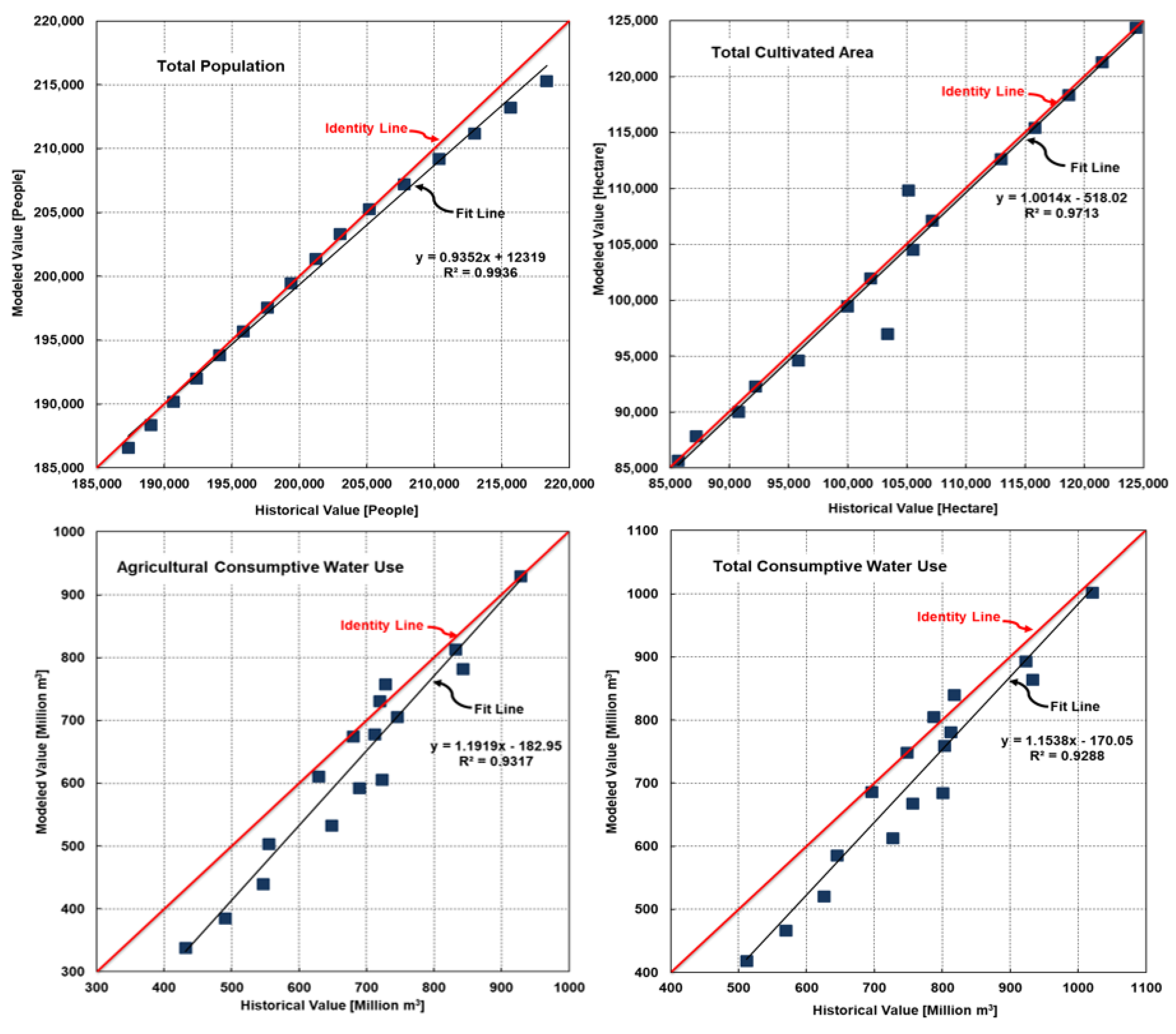
Another representation of the results and findings generated using the developed SE-NM model is demonstrated in Figure 5, where the historical and modeled values for total population, total cultivated area, agricultural consumptive water use, and total consumptive water use during the calibration process are compared. These are in the form of scatter (1:1) plots of population, cultivated area, agricultural consumptive water use, and total consumptive water use for the calibration process. Furthermore, linear regression was used for statistically assessing our model performance. The data were mostly distributed around the identity line (1:1 line or perfect line), indicating clear and close agreement between historical and modeled values (Figure 5). It is clear that in the obtained fit line equations, if the equation is y = βx + α, the slopes (β) are nearer to 1. The values of the slope for the fit-line equations for population, cultivated area, agricultural consumptive water use, and total consumptive water use (0.9352, 1.0014, 1.1919, and 1.1538, respectively) are close to one. Thus, the linear regression equations indicate a close correlation between the modeled and historical data. These outcomes also underscore the accurateness and effectiveness of SE-NM model for assessing these important parameters.
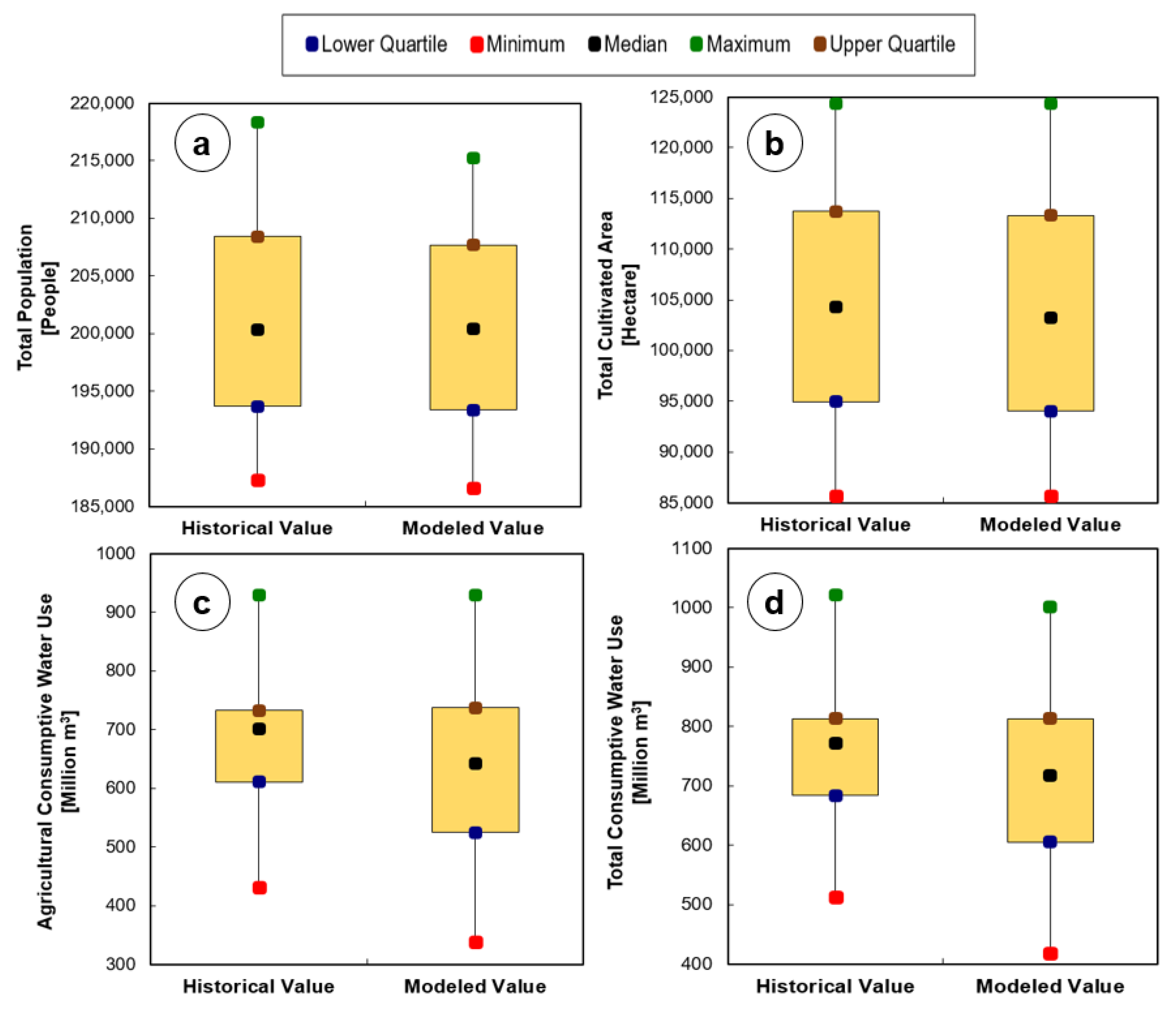
Moreover, to better comprehend and judge the distribution and accuracy of obtained data, results, and model’s capabilities, the modeled and historical actual total population, total cultivated area, agricultural consumptive water use, and total consumptive water use values for calibration dataset were demonstrated and compared in box plots (Figure 6). It is revealed that the both historical actual and modeled values had nearly identical statistical characteristics, such as the minimum, lower quartile, median, upper quartile and maximum, and there was no significant difference. There is a slight difference between the historical and modeled values in both agricultural consumptive water use and total consumptive water use, as shown in Figure 6. However, the values are still close, and this does not affect the model’s accuracy. Moreover, the absence of outliers in the all box plots confirmed the model’s accuracy in describing the behavior of total population, total cultivated area, agricultural consumptive water use, and total consumptive water use. This is also further evidence of the robustness and accuracy of our model, confirming the previous results of statistical performance criteria and 1:1 graphs.
3.2. Sensitivity Analysis Assessment of Scenarios’ Parameters
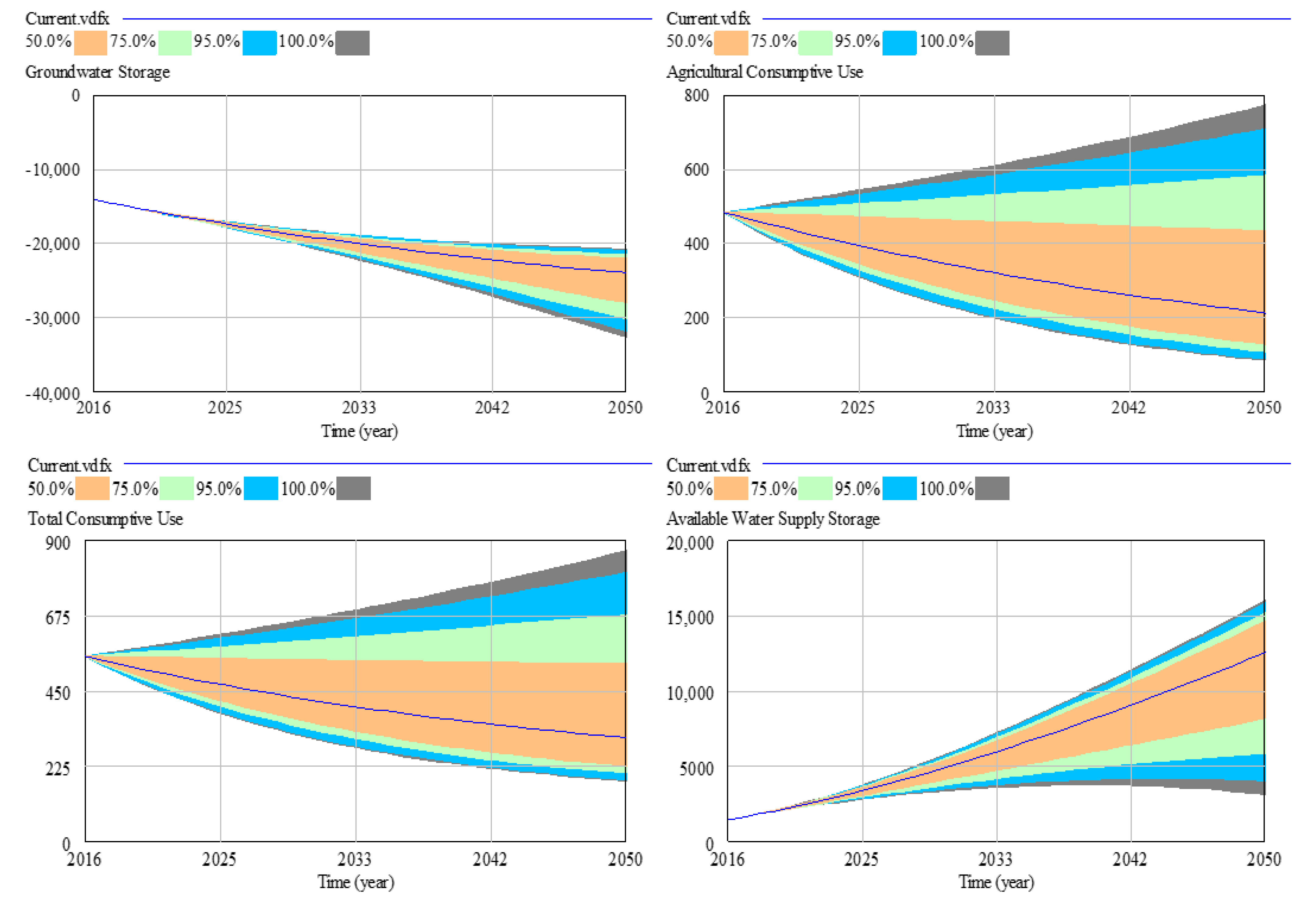
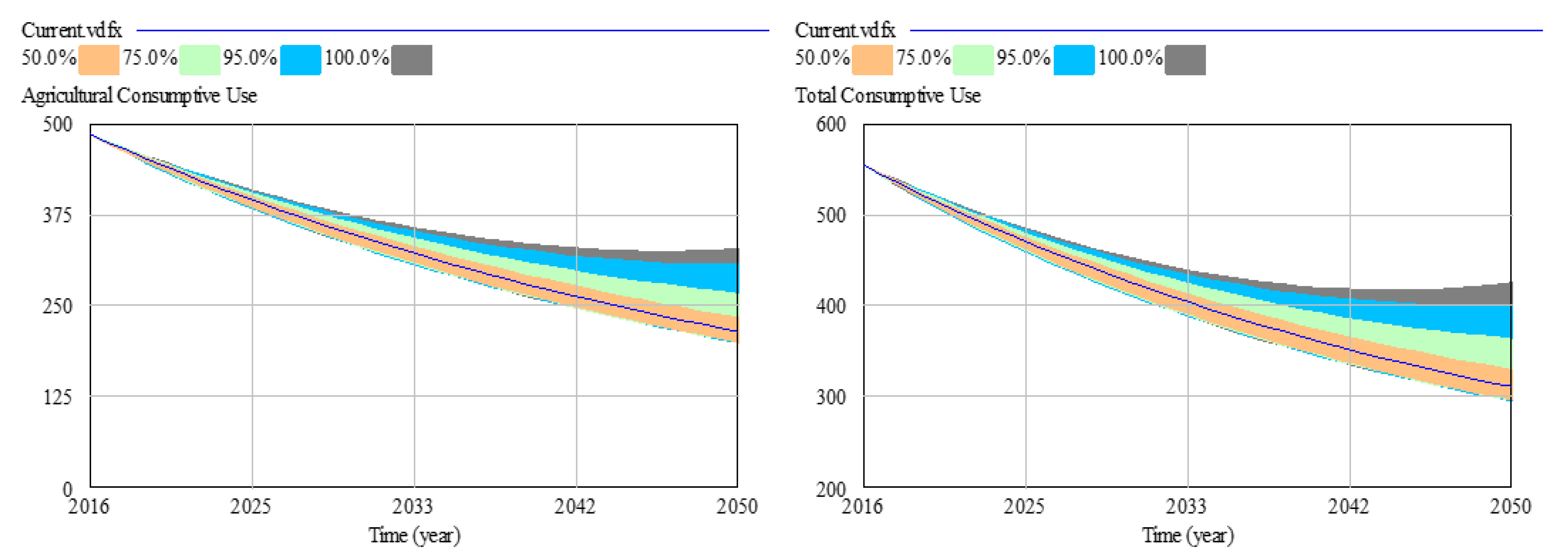
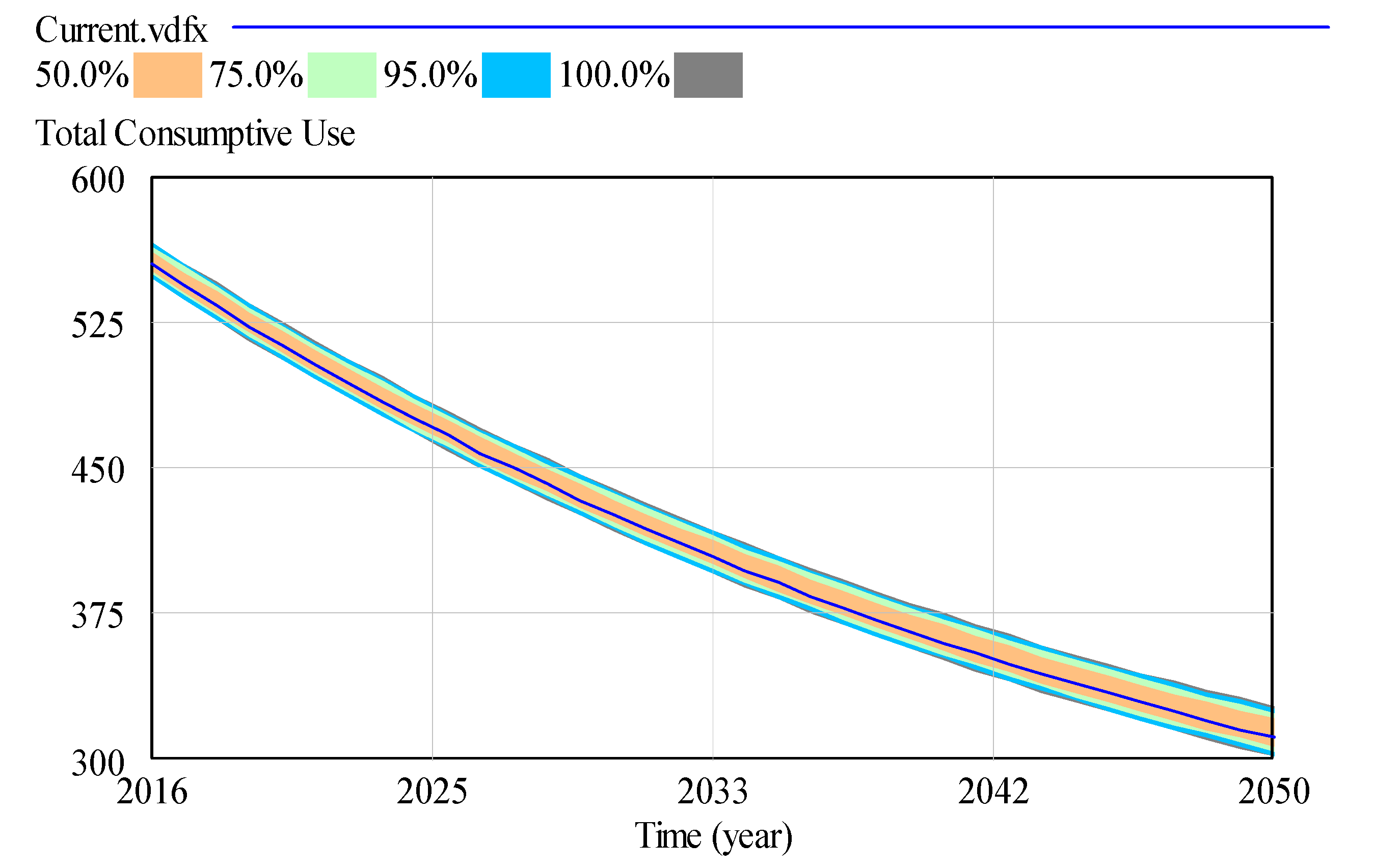
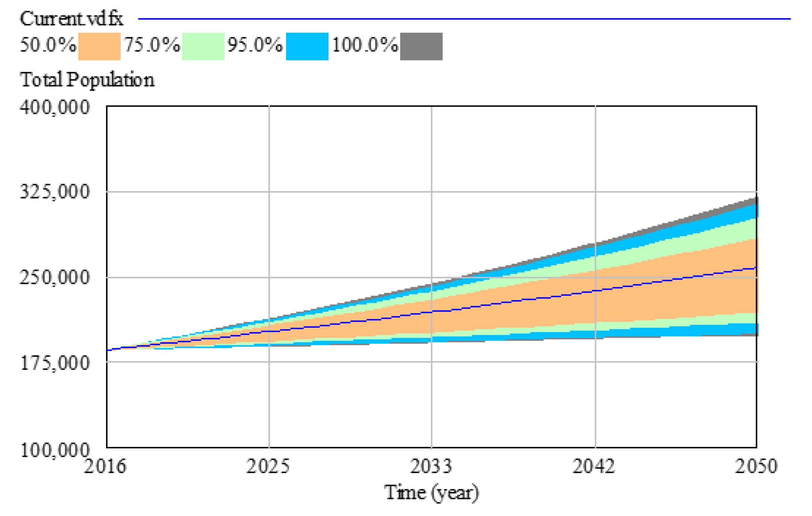
In order to determine which input parameters affect the total population, groundwater storage change, available total water supply (total withdrawals), agricultural consumptive water use, and total consumptive water use, a sensitivity assessment was conducted using the Monte Carlo technique for every input parameter used in the scenarios analysis. The findings of the sensitivity analysis are shown in Figure 7, Figure 8, Figure 9 and Figure 10 for the five main parameters based on several variations. In the legend of the graph, the colors light orange, light green, light blue, and gray demonstrate confidence intervals of 50%, 75%, 95%, and 100%, respectively. In the resulting graph after running Monte Carlo simulation, if the examined parameter visually gives a graph with a broader band, this means that this parameter is more sensitive to the developed model parameter. Thus, sensitivity analysis was done just to verify which input parameters have the most impact on the model and the studied variables. Figure 7, Figure 8, Figure 9 and Figure 10 illustrate only the parameters that most affect some model elements under study (total population, groundwater storage change, available total water supply storage (total withdrawals), agricultural consumptive water use, and total consumptive water use). Cultivated irrigated land change is the most influential parameter for agricultural consumptive water use and total consumptive water use (broadest bands), whereas the livestock growth rate also has a clear impact on each. The importance of Monte Carlo analysis lies in the fact that, just by looking, we can judge the variable’s strength. However, if we want to meticulously quantitatively determine the percentage of contribution or the importance ratio for each variable, we have to combine the SD model with one of the modern methods of quantitative estimation, such as the Fuzzy Logic system or the Cosine Amplitude method, as we mentioned in the future directions and in our detailed review study [37].
However, population growth rate is most important parameter for total population as expected, whereas it has little influence on total water supply change (total withdrawals) and total consumptive water use. Each population growth rate and mining water demand has an impact on the total consumptive water use, but it is not large. Additionally, livestock growth rate has a slight influence on available total water supply. Cultivated irrigated land change has a powerful effect on both groundwater storage and water supply storage, whereas mining water demand affects both marginally. There is also an impact of the mining water demand on the total consumptive water, which may be due to mining water consumption and is considered the third most consumed water category after irrigation and public consumptions [40]. Based on the results of the Monte Carlo sensitivity analysis, total population, groundwater storage change, available total water supply change (total withdrawals), agricultural consumptive water use, and total consumptive water use showed a strong sensitivity to the parameters, especially the cultivated irrigated land change rate. Therefore, cultivated irrigated land change should be taken into consideration as a leverage or influence point when making and developing policies and strategies. As a result, our model can be considered robust, accurate, and appropriate for demonstrating and simulating the sensitivity and dynamic behavior of the variables, parameters, and factors influencing on water system in the SE-NM region.
3.3. Scenarios Analysis and Comparison
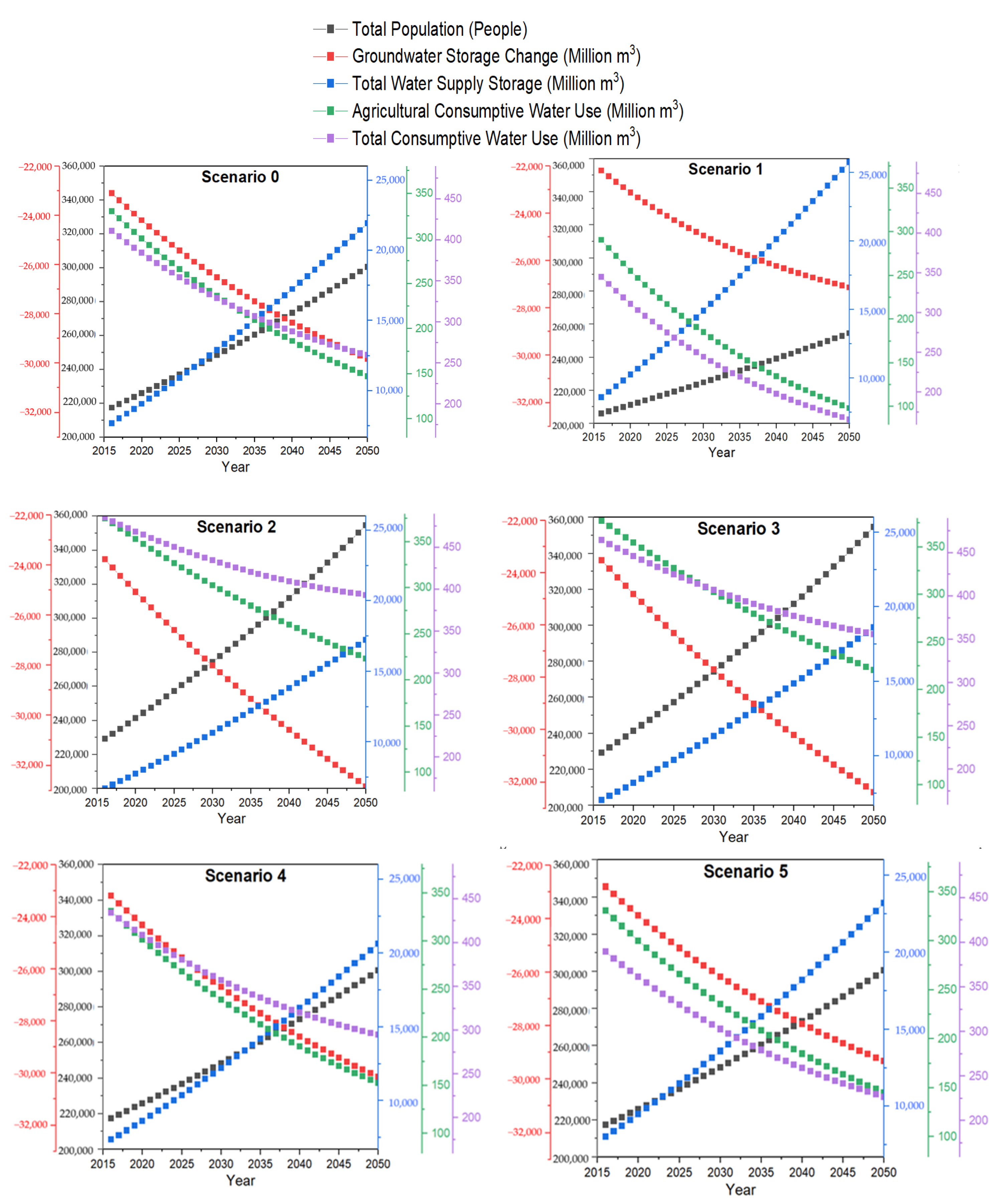
After successfully formulating, developing, checking, and calibrating the SE-NM model, we can analyze its performance under different policy scenarios. Moreover, comparing the results under different used scenarios can provide valuable insights about SE-NM’s water resources situation and development in the future. Additionally, this comparison can benefit water managers and policy makers for planning purposes. The scenarios comparison results can be analyzed from five aspects: total population, groundwater storage change, total water supply storage (total water withdrawals), agricultural consumptive water use, and total consumptive water use. Figure 11 illustrates the plot graphs of these five parameters and Table 4 shows the simulation results under the six scenarios over time from 2016 to 2050.
In all scenarios, the overall average values were −27,187.280 Million m3 groundwater storage change, 240.160 Million m3 agricultural consumptive water use, 339.790 Million m3 total consumptive water use, 14,016.810 Million m3 total water supply storage (total withdrawals), and a 262,458.110 total population between 2016 and 2050. It was shown that there are general decreasing trends in total groundwater storage change, agricultural consumptive water use, and total consumptive water use, but general increasing trends in total water supply storage (total withdrawals) and total population. In other words, overall, there was a decrease of about −30.93% in groundwater storage change, −51.60% in agricultural consumptive water use, and −32.96% in total consumptive water use, whereas there was a rise in total water supply storage change (total withdrawals) of about +180.35% and +41.73% in the total population from 2016 to 2050. In general, Table 4 and Figure 11 illustrate the trends of the most important parameters in the six different scenarios, where there is some similarity, but no symmetry, which confirms and supports the general future trend of the studied parameters.
Population is the principal driver of water consumption and defines and influences various water demands and uses [58,59,60]. In general, there is a closely related relationship between population and water resources: the larger one is, the smaller the other. Accordingly, preserving a balance between them is essential. The findings of all scenarios analyzed in our investigation involving scenario 0 (baseline water demand scenario) show that population growth will continue to rise until 2050, leading to higher consumption rates in all water sectors. According to the used population growth rates, the results of some scenarios are equal to each other for total population (scenario 0 = scenario 5, scenario 1 = scenario 4, and scenario 2 = scenario 3). The total population under scenario 2 is the highest among these six scenarios. It can be observed from Figure 11 and Table 4 that scenario 2 has the highest values of total consumptive water use and lowest values of total water supply storage. The total population in 2050 of scenario 2 is 354,740 people, whereas the corresponding total consumptive water use and total water supply storage change values of this scenario were 394.522 Million m3 and 17,230.101 Million m3, respectively. Based on our outcomes, population growth increases total consumptive water use, which certainly leads to a reduction in available total water supply storage.
Understanding total water consumptive use trends is important to successful and sustainable water management. From Figure 11 and Table 4, it can be seen that the total water consumptive use of all six scenarios (0, 1, 2, 3, 4, and 5) are 259.766 Million m3, 165.059 Million m3, 394.522 Million m3, 355.937 Million m3, 292.841 Million m3, and 227.080 Million m3, respectively, in 2050. The total water consumptive use under scenario 1 is the least among these six scenarios, whereas the highest was scenario 2. The average total water consumptive use values for the scenario 2 were almost 1.34, 1.83, 1.08, 1.23, and 1.47 times that of the values for the scenarios 0, 1, 3, 4, and 5, respectively. Cultivated area growth increases agricultural water use and other water uses rise with total population, which in turn increases total water consumptive use especially in scenario 2 compared to the other scenarios. The results from scenario 2 emphasize the main role of agricultural water use to increase the total water consumptive use and to decrease the available water supply storage (total withdrawals) over time. However, in general, there is a downward trend for total water consumptive use in the period between 2016 and 2050, which follows the prevailing trend in agricultural water use.
Examining groundwater storage trends ensures sustainable management and a stable supply of groundwater. Based on our results, the trends of the six scenarios (0–5) are the same: the groundwater storage change is negatively declining over time over the next 35 years from 2016 to 2050. Figure 11 and Table 4 demonstrate that the groundwater storage change is approximately −29,819.900 Million m3 until 2050, assuming present conditions (scenario 0). Under scenario 1 and 5, the trend of the groundwater storage change decline is lower than that of scenario 0. In scenario 2, the groundwater storage change decreases and reaches about −32,914.145 Million m3 in 2050, and this scenario was the lowest decline compared to the other scenarios for groundwater storage change. In arid and semi-arid regions, such as SE-NM and under drought periods, groundwater is heavily relied upon. Thus, throughout the whole modeling period there is a gradual negative decline in GW storage change. This is because the SE-NM region overlies parts of the Ogallala Aquifer, a fossil aquifer, which has experienced great loss in GW storage (about 3700.440 Million m3) because of the mining industry and agricultural water requirements [61,62,63].
One of the main and central elements in water systems is available water supply storage change, which here is the sum of withdrawals from surface water and groundwater. During the simulation process up to 2050, the total water supply storage change (total withdrawals) has steadily increased with scenario 1 as the largest, followed by scenario 5, scenario 0, scenario 4, scenario 3, and then finally scenario 2. By 2050, the total water supply storage will reach 25,749.546 Million m3 under scenario 1, an increase of 17,146.241 Million m3 compared with that in 2016, whereas the total water supply storage will reach 17,230.101 Million m3 under scenario 2, an increase of only 10,518.920 Million m3 compared with that in 2016. The reason for scenario 1 being the largest can be attributed to total water consumptive use decreasing during the period 2016–2050, and thus the amount of withdrawn water decreases, whereas scenario 2 is the smallest due to the increase in total water consumptive use and therefore showing an increase in the amount of water withdrawn. These results show the extent of the impact of cultivated areas and agricultural water consumption, which in turn influences the total water consumptive use and, consequently, the availability of water supply. Overall, there is an obvious positive upward trend from left to right for all six scenarios as displayed in Figure 11, presented in the total water supply storage. This trend implies that the level of water supply storage change is growing over time.
Agriculture is the biggest consumer of water, not only in the SE-NM region, but also in New Mexico State as a whole, where its consumption is more than 70% of the total water consumption [40]. Reducing cultivated irrigated areas led to a decrease in the average value of agricultural consumptive water use from 230.070 Million m3 (scenario 0) to 180.041 Million m3 (scenario 1), as demonstrated in Table 4 and Figure 11. From the agricultural consumptive water use’s results, it is evident that the trends and values of scenarios 2 and 3 are very close to each other, and they represent the maximum values of agricultural water consumption compared to the other scenarios. This shows the importance of the rate of change of cultivated land. It is also clear that the scenarios 0, 4, and 5 are close to each other, and this is due to using almost the same rate of cultivated land change. In general, and under any of the different scenarios, there is a continuous decrease in agricultural consumptive water use, which in turn reduces total consumptive water use during the entire modeling period. This is primarily because of the reduction trend in SE-NM’s cultivated irrigated areas which have been steadily declining since the 2000s. This result is consistent with the findings of the New Mexico Dynamic Statewide Water Budget (NMDSWB) [45]. The reason for that may be partially due to Settlement Agreement among NM State, the Pecos Valley Artesian Conservancy District, and the U.S. Bureau of Reclamation to offer a more sustained and abundant water supply to the Carlsbad Irrigation District or delivery to Texas. The Settlement Agreement includes decreasing the cultivated irrigated area through the purchase and retirement of thousands of hectares in the SE-NM region, and thus reducing agricultural water use [64]. For example, during the 1990s and 2000s, about 33.674 Million m3 of water rights in the SE-NM region was purchased and retired by the state of New Mexico in accordance with the Pecos Settlement Agreement [65].
3.4. Policy Solutions Suggestions and Recommendations
Overall, the above analysis and scenarios comparison show the dynamic trends of total population, groundwater storage change, total water supply storage change (total withdrawals), agricultural consumptive water use, and total consumptive water use, which provide a general comprehensive understanding and perspective on the SE-NM region’s water demand and supply system. The scenarios that have been simulated have focused particularly on water use and its implications for groundwater storage change. Our analysis of the various scenarios shows that groundwater storage will continue to decline under any scenario, but at a different rate depending on the scenario used. Special management techniques may be useful with regard to withdrawals from groundwater and their monitoring and tracking. Additionally, modernization of groundwater infrastructure (wells), construction records, and updated mapping of the distribution of wells and their classification according to their purpose of use may be beneficial to address groundwater stresses sustainably. Community public participation is also one of the main pillars of any successful water management process. Therefore, improving public awareness and education about groundwater’s importance and its conservation and the fears of not renewing it in light of the inevitable climatic changes would be an effective way to address water challenges in New Mexico [66,67,68]. In addition, through the results obtained in this study from analyzing the different scenarios of agricultural consumer water, we suggest first and foremost that work be done to spread water awareness, especially in agricultural circles. There is a widespread belief among many farmers, irrigators, and farm owners that the use of flood and center pivot sprinkler irrigation systems, the two common types in the SE-NM region [40], and increasing the applied amount of water are the only ways capable of raising crop productivity in quantity and quality. The top concern for farmers, irrigators, or farm owners is to increase application irrigation efficiency in the field, i.e., to pay attention only to the cultivated plant or crop and make sure that irrigation water reaches it. On the other hand, this view is very narrow, because it will cause a change in water balance in the area where the field is located, especially when using center pivot irrigation systems, where the amount of deep percolation is small [69] and the wind drift and evaporation losses are high [70]. Consequently, the aquifer will not be benefited from or recharged.
In general, Gleeson and his colleagues [71] defined groundwater sustainability as “maintaining long-term, dynamically stable storage and flows of high-quality groundwater using inclusive, equitable, and long-term governance and management”. Consequently, the withdrawn groundwater should be less than or equal to the recharged water to ensure stable storage and achieving groundwater sustainability. Therefore, in areas such as the SE-NM region, the artificial recharge of groundwater could be used, which is the direct injection of water through wells into aquifer layers. Furthermore, using modern drip or subsurface drip irrigation systems could be applied to many different crops to give much better results than traditional irrigation systems, whether for flood surface irrigation or center pivot irrigation [72,73,74]. Modern irrigation techniques may be the most efficient in terms of increasing application efficiency and reducing conveyance losses [75]. It has been proven through the obtained results that the changes occurring in the agricultural area have a great influence on controlling the groundwater system. Reducing cultivated area reduces agricultural consumptive water use and thus decreases groundwater withdrawals, but this may affect the production and prices of consumer food commodities. Thus, it is necessary to develop special strategies for crop and food production, taking into account the critical hydrological conditions of this water-scarce region. We propose suites of crop patterns and irrigation systems that benefit farmers economically while reducing water consumption; these options could include high value crops that use more water per unit area but provide proportionately more economic benefit with less overall water use.
Additionally, as a result of the change in livestock growth rate, we find that agricultural consumptive water use has also increased. In order to extend the lifetime of groundwater reserves, changing livestock water use could be implemented by seeking new breeds of dairy cattle, and beef cattle, which consume smaller amounts of water such as traditional Criollo cattle [76,77]. Genetically modified animals and crops may help with water use reduction, but care must be taken to avoid negative human health impacts or introducing new breeds and varieties that are not compatible with local community preferences. Improved water aware management of ranching and grazing that depend on groundwater [78] may have a role in groundwater sustainability, because more than 90% of New Mexico’s land is considered rangeland and suitable for domestic livestock grazing [79]. The change in mining water demand is also significant, and this is because the techniques currently used in the oil and gas industry—hydraulic fracturing and horizontal drilling—consume water heavily, about 16.376 Million m3/year on average in New Mexico [80]. Thus, the development of a mechanism to monitor and follow up on these processes, which accompany oil and gas extraction operations, is necessary. Adopting new water-saving extraction technologies would be beneficial, as would encouraging mining companies to treat and reuse the produced water and use it for various purposes to relieve pressure on groundwater.
From our findings and results, the total water supply storage (total withdrawals) is not static, but in actually showing increasing trends due to several factors, including increased demand associated with increasing regional population. On the other hand, public and domestic water demands were not strongly influential in the over-all total consumptive water use due to the agricultural sector’s dominance over water consumption. However, public and domestic water demands are directly related to population size, so population growth will impact water use in those sectors. As we found in our analysis, the SE-NM region’s population is projected to grow by approximately 83,220 people between 2016 and 2050. There are many negative practices that lead to domestic water misuse in homes, and this may be combated by raising awareness, and installing water-saving devices in homes, such as faucets, toilet tanks, and washing machines that consume less water. Moreover, some policies, practices, and methods must be implemented to reduce the amount of public water used to irrigate public gardens and parks by using water-saving devices, checking for fractures or blockages in sprinkler system heads, repairing leaks in all water delivery pipes, and replacing plants, flowers, and trees that consume large amounts of water with others that consume less water. All of this will certainly reflect positively on water management in a sustainable manner.
4. Challenges and Limitations, and Future Research Directions
This study develops the SE-NM model to evaluate the dynamic behavior of a supply-demand system for water management. This model presents a water use and demand evaluation system and accomplishes qualitative and quantitative assessment, as indicated in our results. This investigation has considered relevant subsystems related to water management as much as possible, such as total population, cultivated area, livestock population, water supply, and water demand subsystems. Nevertheless, this investigation still has certain challenges and limitations. One of the biggest challenges and obstacles facing any modeling process is the availability of accurate, reliable, historical data and its size; especially in our case, data for updated wells, production and operation plans, volume of produced water, its treatment, and reuse is of great importance. There are efforts being made in this regard (accurate mining statistics and data), but they are still less than ambitious. Estimating the overall water applied for the extraction process using hydraulic fracturing is difficult because it varies by well, drilling depth, and geologic properties [80]. Classifications of mining wells and products, cooling systems, and the amounts of water needed to cool electricity generators are important to include. It is necessary to include the social and economic factors affecting water consumption, such as, for example, and not as a limitation, industrial added value, gross domestic product, rural agricultural population, labor force, and income. This will certainly add more depth to recognizing and understanding the nature of the water situation and contribute to making the model more realistic.
The study results provide information and trend sources for the future hydrological development of arid and semi-arid regions. However, the number of variables, relationships, and parameters selected is somewhat limited. Actually, the SE-NM model introduced here is simplified using just fundamental techniques to define the major relationships among the different used elements and parameters in the modeling process. Only the available basic variables and parameters, and simple equations and formulas are used to express performance and behavior. This was intended to simplify the model and make it easier to describe and interpret, and to avoid the problems of running and debugging large models. There is a belief that combining the SD models with other modern modeling techniques will be the main focus of future research trends. This is to increase the certainty and confidence of determining and assessing modeling parameters, involving different features, trends, directions, and patterns of influencing elements and factors to support system dynamic modeling [37]. Moreover, stochastic assessment of flood and drought risks [81], precipitation [82,83], and evapotranspiration [84,85] would be an interesting future direction in terms of multidisciplinary mathematical approaches. Furthermore, it is necessary and beneficial to use big data in modeling tasks. This is the future trend, and therefore it is required to mix, combine, and integrate systems dynamic models with one of the modern modeling systems such as artificial intelligence and machine learning.
5. Summary and Conclusions
Water problems and crises, especially in semi- arid and arid areas, have become more urgent and clearer than other areas and environments. This affects many aspects and sectors of life and requires us to use the most modern and advanced methods to anticipate, understand, and try to solve these problems. The objective of this paper was to investigate, assess, and analyze the dynamic behavior of a water supply and demand system based on system dynamics methodology for achieving sustainable water resources management under different scenarios. The SE-NM region was chosen as a case study and example, and an SD model using Vensim DSS 8.0 software was created. The modeling process involved two phases: the first phase is 2000–2015 and aims to calibrate the developed, whereas the second phase is 2016–2050, which is known as the model prediction phase.
For calibration and behavioral trend tests, historical data were used to choose four essential parameters: total population, total cultivated area, agricultural consumptive water use, and total consumptive water use. The SD model’s performance was evaluated using five statistical performance indicators: R2, RMSE, CRM, IA, and MAPE. The effectiveness and validity of the SD model was confirmed because of the high values of R2 and IA, and the low values of RMSE, CRM, and MAPE. Results revealed that the model can demonstrate the relationships between the different used variables very well and provided good agreement and prediction results. The future total population, groundwater storage change, total water supply storage, agricultural consumptive water use, and total consumptive water use forecasts and trends were examined based on six management scenarios. These policy scenarios focused on low, moderate, high, and combined water use impacts and effects. Under all scenarios, the results show that there are declining trends in groundwater storage change, agricultural consumptive water use, and total consumptive water use, whereas general growing trends in total water supply storage (total withdrawals) and total population were noted from 2016 to 2050.
A sensitivity analysis method, i.e., Monte Carlo, was employed to evaluate the importance of each parameter in the modeling process. The sensitivity analysis of the developed SD model results revealed that the most effective parameter was cultivated irrigated land change. The findings demonstrate that the SD approach is useful to deal with advanced non-linear, and multi-variable water issues. The methodology in this paper may be generalized and extended to other semi-arid and arid regions including the conceptual model, formulation and design, interrelationships, data and parameters, scenarios design and analysis, and comparisons. Overall, it can be concluded that the SD model produced accurate enough outcomes to understand and predict the trend of total population, groundwater storage change, total water supply storage, agricultural consumptive water use, and total consumptive water under semi- arid conditions. There was a gradual negative decline in groundwater storage change, whereas the agricultural area had a great impact on controlling the groundwater system. The continuous decline in agricultural consumptive water use led to reduced total consumptive water use. Among the challenges and limitations are data availability and number of variables in the modeling process. Adding social and economic factors affecting water consumption to the model is a future goal to provide a more detailed description of the dynamic water situation in the SE-NM region.
Supplementary Materials
The following supporting information can be downloaded at: https://www.mdpi.com/article/10.3390/w14121939/s1, model.
Author Contributions
Conceptualization, A.F.M. and A.G.F.; methodology, A.F.M.; software, A.F.M.; validation, A.F.M. and A.G.F.; formal analysis, A.F.M.; investigation, A.F.M.; resources, A.F.M. and A.G.F.; data curation, A.F.M.; writing—original draft preparation, A.F.M.; writing—review and editing, A.F.M. and A.G.F.; visualization, A.F.M.; supervision, A.G.F.; project administration, A.G.F.; funding acquisition, A.G.F. All authors have read and agreed to the published version of the manuscript.
Funding
This research was funded by the National Science Foundation awards no IIA-1301346 and no 1739835, and State of New Mexico Legislature NMWRRI2022.
Institutional Review Board Statement
Not applicable.
Informed Consent Statement
Not applicable.
Data Availability Statement
All data used in this paper are publicly available.
Acknowledgments
The authors would like to thank three anonymous reviewers for their suggestions and comments that greatly helped in improving the manuscript.
Conflicts of Interest
The authors declare no conflict of interest. The funders had no role in the design of the study; in the collection, analyses, or interpretation of data; in the writing of the manuscript, or in the decision to publish the results.
Appendix A
This Appendix illustrates causal loop and stock flow diagrams (SE-NM model) parameter details summary.

Table A1.
The SE-NM model’s subsystems, parameters’ names and types, and data sources.
| Subsystem | Parameter Name | Parameter Type | Data Sources and References |
|---|---|---|---|
| Population | Total population | Stock | [40,45,48,49,51] |
| Population change | Flow | This study | |
| Population growth rate | Variable | [41,45,48,49,51] | |
| Water Supply | Surface water and groundwater storage | Stock | [45] |
| Surface water inflow, groundwater inflow, surface water outflow, groundwater outflow, surface water return flows, groundwater return flows, groundwater evaporation, surface recharge and infiltration, total surface water withdrawals, and total groundwater withdrawals. | Flow | [45,46,48,49,50] | |
| Precipitation, surface water evapotranspiration, land evapotranspiration, natural groundwater inflow, natural groundwater outflow, reservoir evaporation, USGS surface water inflow and outflow, surface runoff, surface water recharge, riparian evaporation, infiltration rate, commerce surface water returns, public surface water returns, irrigated surface water returns, irrigated groundwater returns, mining groundwater returns, industrial surface water returns, total OSE surface water withdrawals, total OSE groundwater withdrawals, commercial surface water withdrawal, domestic surface water withdrawal, public surface water withdrawal, power surface water withdrawal, mining surface water withdrawal, irrigated surface water withdrawal, livestock surface water withdrawal, industrial surface water withdrawal, commercial groundwater withdrawal, domestic groundwater withdrawal, public groundwater withdrawal, power groundwater withdrawal, mining groundwater withdrawal, irrigated groundwater withdrawal, livestock groundwater withdrawal, and industrial groundwater withdrawal. | Variable | [39,45,46,48,49,50] | |
| Water Demand | Available water supply storage change (total withdrawals) | Stock | [48,49,50] |
| Commercial sector water use, domestic sector water use, public sector water use, power sector water use, mining sector water use, irrigated sector water use, livestock sector water use, and industrial sector water us. | Flow | This study | |
| Commercial water demand, domestic water demand, public water demand, power water demand, mining water demand, irrigated water demand, livestock water demand, industrial water demand, total consumptive use, and agricultural consumptive use. | Variable | [40,46,48,49,50] | |
| Livestock | Total livestock population | Stock | [45,48,49] |
| Livestock change | Flow | This study | |
| Livestock growth rate | Variable | [45,48,49] | |
| Cultivated Area | Total cultivated area | Stock | [45,47] |
| Cultivated area change | Flow | This study | |
| Cultivated area growth rate | Variable | [45,47] |
Appendix B
This Appendix demonstrates the main mathematical formulas and expressions of some important variables and parameters (Unit).
- Area Change Rate = Area Growth Rate*Cultivated Area, Units: hectare/year
- Available Fresh Water = INTEG (Total Groundwater Withdrawals + Total Surface Water Withdrawals: Commercial Sector Water Use, Domestic Sector Water use, Industrial Sector Water Use, Irrigated Sector Water Use, Livestock Sector Water Use, Mining Sector Water Use, Power Sector Water Use, and Public Sector Water Use), Units: Million Cubic Meter
- Change in Livestock = Livestock Growth Rate*Livestock Population, Units: animal/year
- Commerce GW Returns = Total Commerce Withdrawals, Commercial Sector Water Use, Units: Million Cubic Meter/year
- Commercial Sector Water Use = Population*Commercial Water Demand, Units: Million Cubic Meter/year
- Cultivated Area = INTEG (Area Change Rate), Units: hectare
- Domestic Sector Water use = Domestic Water Demand*Population, Units: Million Cubic Meter/year
- Groundwater Return Flows = Irrigated GW Returns + Mining GW Returns, Units: Million Cubic Meter/year
- Groundwater Storage = INTEG (Groundwater Return Flows+ GW Inflow + Infiltration + Surface Recharge, GW Evaporation, GW Outflow, Total Groundwater Withdrawals), Units: Million Cubic Meter
- GW Inflow = Groundwater Storage*Natural GW Inflow, Units: Million Cubic Meter/year
- GW Outflow = Groundwater Storage*Natural GW Outflow, Units: Million Cubic Meter/year
- Industrial SW Returns = Total Industrial Withdrawals, Industrial Sector Water Use, Units: Million Cubic Meter/year
- Irrigated Sector Water Use = Cultivated Area*Irrigation Water Demand Units: Million Cubic Meter/year
- Irrigated SW Returns = Total Irrigated Withdrawals, Irrigated Sector Water Use, Units: Million Cubic Meter/year
- Livestock Population = INTEG (Change in Livestock), Units: animal
- Livestock Sector Water Use = Livestock Population*Livestock Water Demand, Units: Million Cubic Meter/year
- Mining GW Returns = Total Mining Withdrawals, Mining Sector Water Use, Units: Million Cubic Meter/year
- Population = INTEG (Population Change), Units: People
- Population Change = Population Growth Rate*Population, Units: People/year
- Public Sector Water Use = Public Water Demand*Population, Units: Million Cubic Meter/year
- Public SW Returns = Total Public Withdrawals, Public Sector Water Use, Units: Million Cubic Meter/year
- Surface Water = INTEG (Surface Water Returns Flows + Surface Water Inflow, Infiltration-Surface Water Outflows, Total Surface Water Withdrawals), Units: Million Cubic Meter
- Surface Water Outflows = SW Evapotranspiration + USGS outflow + Reservoir Evaporation + Land Evapotranspiration, Units: Million Cubic Meter/year
- Surface Water Returns Flows = Commerce GW Returns + Industrial SW Returns + Irrigated SW Returns + Public SW Returns, Units: Million Cubic Meter/year
- Total Commerce Withdrawals = SW with Commercial + GW with Commercial, Units: Million Cubic Meter/year
- Total Consumptive Use = Commercial Sector Water Use + Domestic Sector Water use + Industrial Sector Water Use + Public Sector Water Use + Power Sector Water Use + Mining Sector Water Use + Agricultural Consumptive Use, Units: Million Cubic Meter/year
- Total Domestic Withdrawals = GW with Domestic + SW with Domestic, Units: Million Cubic Meter/year
- Total Industrial Withdrawals = SW with Industrial + GW with Industrial, Units: Million Cubic Meter/year
- Total Irrigated Withdrawals = GW with Irrigated + SW with Irrigation, Units: Million Cubic Meter/year
- Total Livestock Withdrawals = SW with Livestock+ GW with Livestock, Units: Million Cubic Meter/year
- Total Mining Withdrawals = SW with Mining+ GW with Mining, Units: Million Cubic Meter/year
- Total OSE GW with = GW with Commercial + GW with Domestic + GW with Industrial + GW with Irrigated + GW with Livestock + GW with Mining + GW with Power + GW with Public, Units: Million Cubic Meter/year
- Total OSE SW with = SW with Commercial + SW with Domestic + SW with Industrial + SW with Irrigation + SW with Livestock + SW with Mining + SW with Power + SW with Public, Units: Million Cubic Meter/year
- Total Power Withdrawals = SW with Power + GW with Power, Units: Million Cubic Meter/year
- Total Public Withdrawals = GW with Public + SW with Public, Units: Million Cubic Meter/year
References
- Zisopoulou, K.; Zisopoulos, D.; Panagoulia, D. Water Economics: An In-Depth Analysis of the Connection of Blue Water with Some Primary Level Aspects of Economic Theory I. Water 2022, 14, 103. [Google Scholar] [CrossRef]
- Xi, X.; Poh, K.L. Using system dynamics for sustainable water resources management in Singapore. Proc. Comput. Sci. 2013, 16, 157–166. [Google Scholar] [CrossRef] [Green Version]
- Wei, S.; Yang, H.; Song, J.; Abbaspour, K.C.; Xu, Z. System dynamics simulation model for assessing socio-economic impacts of different levels of environmental flow allocation in the Weihe River Basin, China. Eur. J. Oper. Res. 2012, 221, 248–262. [Google Scholar] [CrossRef]
- Li, Y.-H.; Chen, P.-Y.; Lo, W.-H.; Tung, C.-P. Integrated water resources system dynamics modeling and indicators for sustainable rural community. Paddy Water Environ. 2015, 13, 29–41. [Google Scholar] [CrossRef]
- Balali, H.; Viaggi, D. Applying a system dynamics approach for modeling groundwater dynamics to depletion under different economical and climate change scenarios. Water 2015, 7, 5258–5271. [Google Scholar] [CrossRef] [Green Version]
- Subagadis, Y.H.; Grundmann, J.; Schütze, N.; Schmitz, G.H. An integrated approach to conceptualise hydrological and socio-economic interaction for supporting management decisions of coupled groundwater–agricultural systems. Environ. Earth Sci. 2014, 72, 4917–4933. [Google Scholar] [CrossRef]
- Wu, R.S.; Liu, J.S.; Chang, S.Y.; Hussain, F. Modeling of mixed crop field water demand and a smart irrigation system. Water 2017, 9, 885. [Google Scholar] [CrossRef] [Green Version]
- Langsdale, S.; Beall, A.; Carmichael, J.; Cohen, S.; Forster, C. An exploration of water resources futures under climate change using system dynamics modeling. Integr. Assess. 2007, 7, 51–79. [Google Scholar]
- Niazi, A.; Prasher, S.; Adamowski, J.; Gleeson, T. A system dynamics model to conserve arid region water resources through aquifer storage and recovery in conjunction with a dam. Water 2014, 6, 2300–2321. [Google Scholar] [CrossRef] [Green Version]
- Giordano, M. Global groundwater? Issues and solutions. Annu. Rev. Environ. Resour. 2009, 34, 153–178. [Google Scholar] [CrossRef]
- Chaudhuri, S.; Ale, S. Long term (1960–2010) trends in groundwater contamination and salinization in the Ogallala aquifer in Texas. J. Hydrol. 2014, 513, 376–390. [Google Scholar] [CrossRef]
- Ogallala Aquifer Initiative 2011 Report. Natural Resources Conservation Service. United States Department of Agriculture. 2011. Available online: https://www.nrcs.usda.gov/Internet/FSE_DOCUMENTS/stelprdb1048827.pdf (accessed on 5 January 2022).
- Dangar, S.; Asoka, A.; Mishra, V. Causes and implications of groundwater depletion in India: A review. J. Hydrol. 2021, 596, 126103. [Google Scholar] [CrossRef]
- Konikow, L.F.; Kendy, E. Groundwater depletion: A global problem. Hydrogeol. J. 2005, 13, 317–320. [Google Scholar] [CrossRef]
- Sterman, J.D. Business Dynamics: Systems Thinking and Modeling for a Complex World; Irwin/McGraw-Hill: Boston, MA, USA, 2000. [Google Scholar]
- Forrester, J.W. Industrial dynamics: A major breakthrough for decision makers. Harv. Bus. Rev. 1958, 36, 37–66. [Google Scholar]
- Forrester, J.W. System dynamics—A personal view of the first fifty years. Syst. Dynam. Rev. 2007, 23, 345–358. [Google Scholar] [CrossRef]
- Wang, X.-J.; Zhang, J.-Y.; Liu, J.-F.; Wang, G.-Q.; He, R.-M.; Elmahdi, A.; Elsawah, S. Water resources planning and management based on system dynamics: A case study of Yulin city. Environ. Dev. Sustain. 2011, 13, 331–351. [Google Scholar] [CrossRef]
- Winz, I.; Brierley, G.; Trowsdale, S. The use of system dynamics simulation in water resources management. Water Resour. Manag. 2009, 23, 1301–1323. [Google Scholar] [CrossRef]
- Chen, Z.; Wei, S. Application of system dynamics to water security research. Water Resour. Manag. 2014, 28, 287–300. [Google Scholar] [CrossRef]
- Sterman, J.D. System Dynamics Modeling for Project Management; System Dynamics Group Sloan, School of Managment, Massachusetts Institute of Technology: Cambridge, MA, USA, 1992. [Google Scholar]
- Hirsch, G.B.; Levine, R.; Miller, R.L. Using system dynamics modeling to understand the impact of social change initiatives. Am. J. Commun. Psychol. 2007, 39, 239–253. [Google Scholar] [CrossRef]
- Srijariya, W.; Riewpaiboon, A.; Chaikledkaew, U. System dynamic modeling: An alternative method for budgeting. Value Health 2008, 11, S115–S123. [Google Scholar] [CrossRef] [Green Version]
- Guo, H.C.; Liu, L.; Huang, G.H.; Fuller, G.A.; Zou, R.; Yin, Y.Y. A system dynamics approach for regional environmental planning and management: A study for the Lake Erhai Basin. Environ. Manag. 2001, 61, 93–111. [Google Scholar] [CrossRef] [PubMed] [Green Version]
- Sharifi, A.; Kalin, L.; Tajrishy, M. System dynamics approach for hydropower generation assessment in developing watersheds: Case study of karkheh river basin, Iran. J. Hydrol. Eng. 2013, 18, 1007–1017. [Google Scholar] [CrossRef]
- Venkatesan, A.K.; Ahmad, S.; Johnson, W.; Batista, J.R. Salinity reduction and energy conservation in direct and indirect potable water reuse. Desalination 2011, 72, 120–127. [Google Scholar] [CrossRef]
- Venkatesan, A.K.; Ahmad, S.; Johnson, W.; Batista, J.R. System dynamics model to forecast salinity load to the Colorado River due to urbanization within the Las Vegas Valley. Sci. Total Environ. 2011, 409, 2616–2625. [Google Scholar] [CrossRef] [PubMed]
- Tidwell, V.C.; Passell, H.D.; Conrad, S.H.; Thomas, R.P. System dynamics modeling for community-based water planning: Application to the Middle Rio Grande. Aquat. Sci. 2004, 66, 357–372. [Google Scholar] [CrossRef]
- Wang, K.; Davies, E.G.R. A water resources simulation gaming model for the Invitational Drought Tournament. J. Environ. Manag. 2015, 160, 167–183. [Google Scholar] [CrossRef]
- Bai, Y.; Langarudi, S.P.; Fernald, A.G. System Dynamics Modeling for Evaluating Regional Hydrologic and Economic Effects of Irrigation Efficiency Policy. Hydrology 2021, 8, 61. [Google Scholar] [CrossRef]
- Ahmad, S.; Simonovic, S.P. System dynamics modeling of reservoir operations for flood management. J. Comput. Civ. Eng. 2000, 14, 190–198. [Google Scholar] [CrossRef]
- Ryu, J.H.; Contor, B.; Johnson, G.; Allen, R.; Tracy, J. System dynamics to sustainable water resources management in the eastern Snake Plain Aquifer under water supply uncertainty. J. Am. Water Resour. Assoc. 2012, 48, 1204–1220. [Google Scholar] [CrossRef]
- Elmahdi, A.; Malano, H.; Etchells, T. Using system dynamics to model water-reallocation. Environmentalist 2007, 27, 3–12. [Google Scholar] [CrossRef]
- Zomorodian, M.; Lai, S.H.; Homayounfar, M.; Shaliza, I.; Pender, G. Development and application of coupled system dynamics and game theory: A dynamic water conflict resolution method. PLoS ONE 2017, 12, e0188489. [Google Scholar] [CrossRef] [PubMed] [Green Version]
- Barati, A.A.; Azadi, H.; Scheffran, J. A system dynamics model of smart groundwater governance. Agric. Water Manag. 2019, 221, 502–518. [Google Scholar] [CrossRef]
- Yang, J.; Lei, K.; Khu, S.; Meng, W. Assessment of water resources carrying capacity for sustainable development based on a system dynamics model: A case study of Tieling City, China. Water Resour. Manag. 2015, 29, 885–899. [Google Scholar] [CrossRef]
- Mashaly, A.F.; Fernald, A.G. Identifying Capabilities and Potentials of System Dynamics in Hydrology and Water Resources as a Promising Modeling Approach for Water Management. Water 2020, 12, 1432. [Google Scholar] [CrossRef]
- U.S. Census Bureau. Quick Facts. 2010. Available online: https://www.census.gov/quickfacts/fact/table/leacountynewmexico,NM/POP010210 (accessed on 11 January 2021).
- PRISM Climate Group. Oregon State University. 2018. Available online: http://prism.oregonstate.edu (accessed on 19 February 2021).
- Magnuson, M.L.; Valdez, J.M.; Lawler, C.R.; Nelson, M.; Petronis, L. New Mexico Water Use by Categories 2015; New Mexico State Engineer: Santa Fe, NM, USA, 2019. [Google Scholar]
- Richardson, G.P.; Pugh, A.L., III. Introduction to System Dynamics Modeling with DYNAMO; MIT Press: Cambridge, MA, USA, 1981. [Google Scholar]
- Ventana Systems Inc. VensimDSS; Ventana Systems Inc.: Harvard, MA, USA, 2019. [Google Scholar]
- Panagoulia, D.; Vlahogianni, E.I. Nonlinear dynamics and recurrence analysis of extreme precipitation for observed and general circulation model generated climates. Hydrol. Process. 2014, 28, 2281–2292. [Google Scholar] [CrossRef]
- Mirchi, A.; Madani, K.; Watkins, D.; Ahmad, S. Synthesis of system dynamics tools for holistic conceptualization of water resources problems. Water Resour. Manag. 2012, 26, 2421–2442. [Google Scholar] [CrossRef]
- Peterson, K.; Hanson, A.; Roach, J.; Randall, J.; Thomson, B. A Dynamic Statewide Water Budget for New Mexico: Phase III–Future Scenario Implementation; New Mexico Water Resources Research Institute, New Mexico State University: Las Cruces, NM, USA, 2019. [Google Scholar]
- USGS (United States Geological Survey). USGS Water Data for USA. 2015. Available online: http://waterdata.usgs.gov/nwis (accessed on 3 February 2021).
- USDA (United States Department of Agriculture). 2015 New Mexico Agricultural Statistics: USDA NASS NM Field Office. Available online: https://www.nass.usda.gov/Statistics_by_State/New_Mexico/Publications/index.php (accessed on 16 May 2021).
- Longworth, J.W.; Valdez, J.M.; Magnuson, M.L.; Sims, A.; Elisa, J.; Keller, J. New Mexico Water Use by Categories 2005; New Mexico State Engineer: Santa Fe, NM, USA, 2008. [Google Scholar]
- Longworth, J.W.; Valdez, J.M.; Magnuson, M.L.; Richard, K. New Mexico Water Use by Categories 2010; New Mexico State Engineer: Santa Fe, NM, USA, 2013. [Google Scholar]
- Wilson, B.; Lucero, A.A.; Romero, J.T.; Romero, P.J. Water Use by Categories in New Mexico Counties and River Basins, and Irrigated Acreage in 2000; New Mexico Office of the State Engineer: Santa Fe, NM, USA, 2003; p. 173. [Google Scholar]
- UNM BBER (University of New Mexico Bureau of Business and Economic Research). Data Page on the UNM BBER Website. Historical Demographic Tables and Maps. Available online: https://bber.unm.edu/historical-comparisons (accessed on 6 December 2020).
- Miehle, P.; Livesley, S.J.; Liw, C.; Feikemaz, P.M.; Adams, M.A.; Arndt, S.K. Quantifying uncertainty from large-scale model predictions of forest carbon dynamics. Glob. Change Biol. 2006, 12, 1421–1434. [Google Scholar] [CrossRef]
- Arbat, G.; Puig-Bargues, J.; Barragan, J.; Bonany, J.; Ramirez de Cartagena, F. Monitoring soil water status for micro-irrigation management versus modeling approach. Biosyst. Eng. 2008, 100, 286–296. [Google Scholar] [CrossRef]
- Legates, D.R.; McCabe, G.J., Jr. Evaluating the use of “goodness-of fit” measures in hydrologic and hydroclimatic model validation. Water Resour. Res. 1999, 35, 233–241. [Google Scholar] [CrossRef]
- Loague, K.; Green, R.E. Statistical and graphical methods for evaluating solute transport models: Overview and application. J. Contam. Hydrol. 1991, 7, 51–73. [Google Scholar] [CrossRef]
- De Myttenaere, A.; Golden, B.; Le Grand, B.; Rossi, F. Mean absolute percentage error for regression models. Neurocomputing 2016, 192, 38–48. [Google Scholar] [CrossRef] [Green Version]
- Willmott, C.J. On the validation of models. Phys. Geogr. 1981, 2, 184–194. [Google Scholar] [CrossRef]
- Wu, G.; Li, L.; Ahmad, S.; Chen, X.; Pan, X. A dynamic model for vulnerability assessment of regional water resources in arid areas: A case study of Bayingolin, China. Water Resour. Manag. 2013, 27, 3085–3101. [Google Scholar] [CrossRef]
- Davies, E.G.; Simonovic, S.P. Global water resources modeling with an integrated model of the social–economic–environmental system. Adv. Water Resour. 2011, 34, 684–700. [Google Scholar] [CrossRef]
- Simonovic, S.P. Managing Water Resources: Methods and Tools for a Systems Approach; UNESCO Publishing: Paris, France, 2009. [Google Scholar]
- Tillery, A.C. Current (2004-07) Conditions and Changes in Ground-water Levels from Predevelopment to 2007, Southern High Plains Aquifer, Southeast New Mexico, Lea County Underground Water Basin; U.S. Geological Survey Scientific Investigations Map 3044; U.S. Geological Survey: Reston, VA, USA, 2008; 1 sheet. [Google Scholar]
- Ketchum, D.; Newton, T.B.; Phillips, F. Statewide Water Assessment: Recharge Data Compilation and Recharge Area Identification for the State of New Mexico. Socorro, NM. 2015. Available online: https://nmwrri.nmsu.edu/wp-content/SWWA/Reports/Newton/June%202015%20FINAL/Recharge_Final_Report_2014-2015.pdf (accessed on 27 June 2021).
- Rinehart, A.J.; Mamer, E.; Kludt, T.; Felix, B.; Pokorny, C.; Timmons, S. Groundwater level and storage changes in alluvial basins in the Rio Grande Basin, New Mexico. In New Mexico Water Resources Research Institute Technical Completion Report; New Mexico Bureau of Geology and Mineral Resources: Socorro, NM, USA, 2016; 41p. [Google Scholar]
- Elhassan, A.; Carron, J.; McCord, J.; Barroll, P. Evaluation of the Pecos River Carlsbad Settlement Agreement Using the Pecos River Decision Support System. Doctoral Dissertation, Colorado State University, Fort Collins, CO, USA, 2006. [Google Scholar]
- Blaine, T.; Dixon, D.K. New Mexico Office of the State Engineer/Interstate Stream Commission Annual Reports for Fiscal Year 2011–2012, Fiscal Year 2012–2013, Fiscal Year 2013–2014, 2015. Available online: https://www.ose.state.nm.us/Plans/AnnualReports/2011_2014/11-14-annual-rpt.pdf (accessed on 2 August 2021).
- Rawling, G.C. A hydrogeologic investigation of Curry and Roosevelt Counties, New Mexico. Aquifer Mapping Program, New Mexico Bureau of Geology and Mineral Resources. 2016. Available online: https://www.currycounty.org/home/showpublisheddocument/1792/636772758839300000 (accessed on 18 March 2022).
- Geery, E. A Summary of Stakeholder Perspectives on New Mexico’s Water Resources and Data Needs 2021. New Mexico Interstate Stream Commission. Available online: https://newmexicowaterdata.org/wp-content/uploads/2021/08/StakeholderPerspectives_August2021.pdf (accessed on 20 March 2022).
- 2018 New Mexico State Water Plan. New Mexico Interstate Stream Commission. Available online: https://drought.unl.edu/archive/plans/Water/state/NM_2018.pdf (accessed on 29 March 2022).
- Taghvaeian, S.; Frazier, R.S.; Livingston, D.; Fox, G.; The Ogallala Aquifer. Oklahoma Cooperative Extension Service publication BAE-1531. March 2017. Available online: https://extension.okstate.edu/fact-sheets/the-ogallala-aquifer.html (accessed on 16 October 2021).
- Stambouli, T.; Martínez-Cob, A.; Faci, J.M.; Howell, T.; Zapata, N. Sprinkler evaporation losses in alfalfa during solid-set sprinkler irrigation in semiarid areas. Irrig. Sci. 2013, 31, 1075–1089. [Google Scholar] [CrossRef] [Green Version]
- Gleeson, T.; Cuthbert, M.; Ferguson, G.; Perrone, D. Global groundwater sustainability, resources, and systems in the Anthropocene. Annu. Rev. Earth Planet. Sci. 2020, 48, 431–463. [Google Scholar] [CrossRef] [Green Version]
- Yazar, A.; Sezen, S.M.; Sesveren, S. LEPA and trickle irrigation of cotton in the Southeast Anatolia Project (GAP) area in Turkey. Agric. Water Manag. 2002, 54, 189–203. [Google Scholar] [CrossRef]
- Ayars, J.E.; Fulton, A.; Taylor, B. Subsurface drip irrigation in California—Here to stay? Agric. Water Manag. 2015, 157, 39–47. [Google Scholar] [CrossRef]
- Şimşek, M.; Kaçıra, M.; Tonkaz, T. The effects of different drip irrigation regimes on watermelon [Citrullus lanatus (Thunb.)] yield and yield components under semi-arid climatic conditions. Aust. J. Agric. Res. 2004, 55, 1149–1157. [Google Scholar] [CrossRef]
- Evans, R.G.; Sadler, E.J. Methods and technologies to improve efficiency of water use. Water Resour. Res. 2008, 44, W00E04. [Google Scholar] [CrossRef]
- McIntosh, M.M.; Cibils, A.F.; Estell, R.E.; Nyamuryekung’e, S.; González, A.L.; Gong, Q.; Cao, H.; Spiegal, S.A.; Soto-Navarro, S.A.; Blair, A.D. Weight Gain, Grazing Behavior and Carcass Quality of Desert Grass-fed Rarámuri Criollo vs. Crossbred Steers. Livest. Sci. 2021, 249, 104511. [Google Scholar] [CrossRef]
- Estell, R. The Genesis of the Jornada Criollo Cattle Program. J. Arid Environ. 2021, 193, 10453. [Google Scholar] [CrossRef]
- New Mexico Interstate Stream Commission (NMISC). Pecos River Basin Study New Mexico, Evaluation of Future Water Supply and Demand for Irrigated Agriculture in the Pecos Basin in New Mexico. 2021. Available online: https://www.usbr.gov/watersmart/bsp/docs/finalreport/Pecos/PRNMB-final-9-20-2021.pdf (accessed on 14 November 2021).
- Allison, C.D.; Ashcroft, N. New Mexico range plants (Circular 374). College of Agricultural, Consumer and Environmental Sciences, New Mexico State University, 2011. Available online: https://aces.nmsu.edu/pubs/_circulars/CR374_SM.pdf (accessed on 26 November 2021).
- Valder, J.F.; McShane, R.R.; Thamke, J.N.; McDowell, J.S.; Ball, G.P.; Houston, N.A.; Galanter, A.E. Estimates of Water Use Associated with Continuous Oil and Gas Development in the Permian Basin, Texas and New Mexico, 2010–2019; Scientific Investigations Report 2021–5090; U.S. Department of the Interior—U.S. Geological Survey: Reston, VA, USA, 2021; 27p. [Google Scholar]
- Le Cam, L. A stochastic description of precipitation. In Proceedings of the Fourth Berkeley Symposium on Mathematical Statistics and Probability, Oakland, CA, USA, 20 June–30 July 1960; University of California Press: Berkeley, CA, USA, 1961; Volume 3, pp. 165–186. [Google Scholar]
- Park, J.; Onof, C.; Kim, D. A hybrid stochastic rainfall model that reproduces some important rainfall characteristics at hourly to yearly timescales. Hydrol. Earth Syst. Sci. 2019, 23, 989–1014. [Google Scholar] [CrossRef] [Green Version]
- Unami, K.; Abagale, F.K.; Yangyuoru, M.; Badiul Alam, A.H.M.; Kranjac-Berisavljevic, G. A stochastic differential equation model for assessing drought and flood risks. Stoch. Environ. Res. Risk Assess. 2010, 24, 725–733. [Google Scholar] [CrossRef]
- De Assis, J.P.; de Sousa, R.P.; Martins, W.R.; Linhares, P.C.F.; de Almeida Cardoso, E.; de Araujo Paula, J.A.; de Freitas Almeida dos Santos, M.; de Sousa, I.L.B.; de Araujo, M.B. Stochastic modeling of reference evapotranspiration in arid and semi-arid zones. Aust. J. Crop Sci. 2020, 14, 204–211. [Google Scholar] [CrossRef]
- Tu Pham, M.; Vernieuwe, H.; de Baets, B.; Verhoest, N.E.C. A coupled stochastic rainfall-evapotranspiration model for hydrological impact analysis. Hydrol. Earth Syst. Sci. 2018, 22, 1263–1283. [Google Scholar] [CrossRef] [Green Version]
Figure 1.
Map of the study location SE-NM, USA, showing its land cover classes.

Figure 2.
Water’s withdrawals for different use categories for the SE-NM region in 2011–2015.

Figure 3.
Casual loop diagram (CLD) or conceptual model of the SE-NM model [CLD’s parameter details summary is explained in Appendix A].
Figure 3.
Casual loop diagram (CLD) or conceptual model of the SE-NM model [CLD’s parameter details summary is explained in Appendix A].

Figure 4.
Stock and flow diagram (SFD) used to create the SE-NM model [SFD’s parameter details summary is explained in Appendix A, where SW with: Surface Water Withdrawal; GW with: Groundwater Withdrawal].
Figure 4.
Stock and flow diagram (SFD) used to create the SE-NM model [SFD’s parameter details summary is explained in Appendix A, where SW with: Surface Water Withdrawal; GW with: Groundwater Withdrawal].

Figure 5.
Performance of the developed SE-NM model during calibration processing the four selected variables: total population, total cultivated area, agricultural consumptive water use, and total consumptive water use [identity line = 1:1 line].
Figure 5.
Performance of the developed SE-NM model during calibration processing the four selected variables: total population, total cultivated area, agricultural consumptive water use, and total consumptive water use [identity line = 1:1 line].

Figure 6.
Box plots of historical and modeled values for the four selected parameters: (a) total population, (b) total cultivated area, (c) agricultural consumptive water use, and (d) total consumptive water use during calibration process.
Figure 6.
Box plots of historical and modeled values for the four selected parameters: (a) total population, (b) total cultivated area, (c) agricultural consumptive water use, and (d) total consumptive water use during calibration process.

Figure 7.
Monte Carlo sensitivity analysis results under cultivated area change rate [100% represents no change from current trend].
Figure 7.
Monte Carlo sensitivity analysis results under cultivated area change rate [100% represents no change from current trend].

Figure 8.
Monte Carlo sensitivity analysis results under livestock change rate.

Figure 9.
Monte Carlo sensitivity analysis results under mining water demand.

Figure 10.
Monte Carlo sensitivity analysis results under population growth rate.

Figure 11.
The behavior of the five main important parameters: total population, groundwater storage change, total water supply storage (total withdrawals), agricultural consumptive water use, and total consumptive water use, under six different scenarios.
Figure 11.
The behavior of the five main important parameters: total population, groundwater storage change, total water supply storage (total withdrawals), agricultural consumptive water use, and total consumptive water use, under six different scenarios.

Table 1.
Main components of system dynamics model using Vensim software.
| Name and Vensim Form | Concept | Mathematical Expression |
|---|---|---|
Level (Stock or State) | It indicates the primary quantity to be accumulated. Over time, the values grow or decrease. | Level = A(t). It is a dependent variable (unknown variable); time or t is normally an independent one. |
Rate (Flow) | Express actions and operations that increase or decrease stock value over time. It denotes change per unit time of stock.  symbolize the sources or sinks. symbolize the sources or sinks. | Rate = dA/dt |
Arrow (Connector) | Express, represent, and connect a direction between two variables, and transport information from variable to variable. | Physical principles governing the phenomena, assumptions or hypotheses we have made. |
| Variable Auxiliary Constant  | It is generally a flow change, and expresses auxiliary variable used to store and supports constant variables. Over time, constants do not change. | k This is an equation parameter. |
Table 2.
Maximum, minimum, standard deviation, and initial values of parameters used in the Monte Carlo analysis.
Table 2.
Maximum, minimum, standard deviation, and initial values of parameters used in the Monte Carlo analysis.
| Parameters | Unit | INIT | MINI | MAXI | SDE |
|---|---|---|---|---|---|
| Population Growth Rate | 1/year | 9.58 × 10⁻³ | 1.80 × 10⁻³ | 1.61 × 10⁻² | 5.85 × 10⁻³ |
| Cultivated Growth Rate | 1/year | −2.45 × 10⁻² | −5.45 × 10⁻² | 1.52 × 10⁻² | 1.92 × 10⁻² |
| Livestock Growth Rate | 1/year | −9.59 × 10⁻³ | −1.06 × 10⁻¹ | 5.49 × 10⁻² | 4.49 × 10⁻² |
| Public Water Demand | Mm3/person/year | 1.98 × 10⁻⁴ | 1.97 × 10⁻⁴ | 2.38 × 10⁻⁴ | 1.16 × 10⁻⁵ |
| Domestic Water Demand | Mm3/person/year | 1.94 × 10⁻⁵ | 1.81 × 10⁻⁵ | 2.22 × 10⁻⁵ | 1.28 × 10⁻⁶ |
| Mining Water Demand | Mm3/person/year | 9.20 × 10⁻⁵ | 5.30 × 10⁻⁵ | 1.55 × 10⁻⁴ | 3.01 × 10⁻⁵ |
INIT: initial value; MINI: minimum value; MAXI: maximum value; SDE: standard deviation value.
Table 3.
Statistical performance of the developed SE-NM model during calibration stage.
| Selected Model Parameters | Statistical Performance Criteria | ||||
|---|---|---|---|---|---|
| R2 | RMSE | CRM | MAPE | IA | |
| Total Population (People) | 0.9936 | 1173.94 | −0.0036 | 0.3722 | 0.9958 |
| Total Cultivated Area (Hectare) | 0.9713 | 2046.93 | −0.0035 | 1.0110 | 0.9924 |
| Agricultural Consumptive Water Use (Million m3) | 0.9317 | 70.5854 | −0.0764 | 9.3915 | 0.9397 |
| Total Consumptive Water Use (Million m3) | 0.9288 | 70.1657 | −0.0696 | 8.3152 | 0.9409 |
R2: coefficient of determination; RMSE: root mean square error; CRM: coefficient of residual mass; MAPE: mean absolute percentage error; IA: index of agreement.
Table 4.
Simulation results for total population, groundwater storage change, total water supply storage (total withdrawals), agricultural consumptive water use, and total consumptive water use under the six scenarios.
Table 4.
Simulation results for total population, groundwater storage change, total water supply storage (total withdrawals), agricultural consumptive water use, and total consumptive water use under the six scenarios.
| Year | Scenarios | |||||
|---|---|---|---|---|---|---|
| 0 | 1 | 2 | 3 | 4 | 5 | |
| Total Population (People) | ||||||
| 2016 | 217,320 | 206,054 | 229,162 | 229,162 | 217,320 | 217,320 |
| 2020 | 225,769 | 211,235 | 241,250 | 241,250 | 225,769 | 225,769 |
| 2025 | 236,794 | 217,895 | 257,261 | 257,261 | 236,794 | 236,794 |
| 2030 | 248,357 | 224,765 | 274,335 | 274,335 | 248,357 | 248,357 |
| 2035 | 260,485 | 231,852 | 292,542 | 292,542 | 260,485 | 260,485 |
| 2040 | 273,206 | 239,162 | 311,958 | 311,958 | 273,206 | 273,206 |
| 2045 | 286,547 | 246,702 | 332,662 | 332,662 | 286,547 | 286,547 |
| 2050 | 300,540 | 254,481 | 354,740 | 354,740 | 300,540 | 300,540 |
| Groundwater Storage Change (Million m3) | ||||||
| 2016 | −23,097.823 | −22,495.406 | −23,744.261 | −23,638.242 | −23,201.124 | −22,994.525 |
| 2020 | −24,196.331 | −23,404.882 | −25,060.276 | −24,924.132 | −24,328.062 | −24,064.612 |
| 2025 | −25,428.424 | −24,377.641 | −26,601.946 | −26,425.967 | −25,597.257 | −25,259.796 |
| 2030 | −26,521.741 | −25,195.014 | −28,038.307 | −27,819.962 | −26,729.376 | −26,314.174 |
| 2035 | −27,493.257 | −25,881.566 | −29,379.115 | −29,115.341 | −27,741.542 | −27,244.902 |
| 2040 | −28,358.043 | −26,457.727 | −30,633.108 | −30,321.124 | −28,649.112 | −28,067.046 |
| 2045 | −29,129.717 | −26,941.206 | −31,808.965 | −31,445.364 | −29,465.645 | −28,793.813 |
| 2050 | −29,819.906 | −27,346.845 | −32,914.145 | −32,495.667 | −30,202.926 | −29,437.064 |
| Total Water Supply Storage Change [Total Withdrawals] (Million m3) | ||||||
| 2016 | 7687.724 | 8603.336 | 6711.203 | 7054.311 | 7353.034 | 8022.134 |
| 2020 | 9056.703 | 10,257.06 | 7756.123 | 8198.834 | 8627.846 | 9485.151 |
| 2025 | 10,912.046 | 12,501.413 | 9153.210 | 9728.633 | 10,359.215 | 11,463.714 |
| 2030 | 12,906.921 | 14,913.210 | 10,639.072 | 11,356.812 | 12,223.303 | 13,588.912 |
| 2035 | 15,022.164 | 17,465.323 | 12,201.225 | 13,071.421 | 14,200.578 | 15,841.103 |
| 2040 | 17,240.186 | 20,134.501 | 13,827.924 | 14,861.147 | 16,273.256 | 18,203.232 |
| 2045 | 19,545.303 | 22,901.489 | 15,507.914 | 16,715.124 | 18,425.622 | 20,659.730 |
| 2050 | 21,923.812 | 25,749.546 | 17,230.101 | 18,623.012 | 20,643.442 | 23,197.046 |
| Agricultural Consumptive Water Use (Million m3) | ||||||
| 2016 | 329.864 | 287.838 | 377.733 | 376.676 | 330.922 | 328.859 |
| 2020 | 299.734 | 252.902 | 354.956 | 353.675 | 301.015 | 298.534 |
| 2025 | 265.992 | 215.263 | 328.442 | 326.903 | 267.531 | 264.574 |
| 2030 | 236.131 | 183.361 | 303.949 | 302.174 | 237.906 | 234.524 |
| 2035 | 209.703 | 156.312 | 281.321 | 279.331 | 211.693 | 207.93 |
| 2040 | 186.307 | 133.37 | 260.415 | 258.229 | 188.494 | 184.392 |
| 2045 | 165.593 | 113.903 | 241.099 | 238.734 | 167.957 | 163.557 |
| 2050 | 147.249 | 97.3776 | 223.250 | 220.725 | 149.774 | 145.111 |
| Total Consumptive Water Use (Million m3) | ||||||
| 2016 | 411.224 | 342.641 | 488.375 | 464.022 | 434.373 | 388.130 |
| 2020 | 384.258 | 309.082 | 471.434 | 445.629 | 408.488 | 360.110 |
| 2025 | 354.643 | 273.215 | 452.651 | 424.961 | 380.252 | 329.157 |
| 2030 | 329.112 | 243.14 | 436.401 | 406.739 | 356.132 | 302.260 |
| 2035 | 307.224 | 217.976 | 422.564 | 390.836 | 335.692 | 278.974 |
| 2040 | 288.590 | 196.977 | 411.032 | 377.134 | 318.548 | 258.906 |
| 2045 | 272.871 | 179.516 | 401.712 | 365.531 | 304.363 | 241.709 |
| 2050 | 259.766 | 165.059 | 394.522 | 355.937 | 292.841 | 227.080 |
Publisher’s Note: MDPI stays neutral with regard to jurisdictional claims in published maps and institutional affiliations. |
© 2022 by the authors. Licensee MDPI, Basel, Switzerland. This article is an open access article distributed under the terms and conditions of the Creative Commons Attribution (CC BY) license (https://creativecommons.org/licenses/by/4.0/).
Share and Cite
MDPI and ACS Style
Mashaly, A.F.; Fernald, A.G. Analyzing and Assessing Dynamic Behavior of a Physical Supply and Demand System for Sustainable Water Management under a Semi-Arid Environment. Water 2022, 14, 1939. https://doi.org/10.3390/w14121939
AMA Style
Mashaly AF, Fernald AG. Analyzing and Assessing Dynamic Behavior of a Physical Supply and Demand System for Sustainable Water Management under a Semi-Arid Environment. Water. 2022; 14(12):1939. https://doi.org/10.3390/w14121939
Chicago/Turabian StyleMashaly, Ahmed F., and Alexander G. Fernald. 2022. "Analyzing and Assessing Dynamic Behavior of a Physical Supply and Demand System for Sustainable Water Management under a Semi-Arid Environment" Water 14, no. 12: 1939. https://doi.org/10.3390/w14121939
Note that from the first issue of 2016, this journal uses article numbers instead of page numbers. See further details here.