Article

Agricultural Irrigation Effects on Hydrological Processes in the United States Northern High Plains Aquifer Simulated by the Coupled SWAT-MODFLOW System

by
Sijal Dangol
1,
Xuesong Zhang
2,*,
Xin-Zhong Liang
1,3 and
Fernando Miralles-Wilhelm
4,5
1
Department of Atmospheric and Oceanic Science, University of Maryland, College Park, MD 20742, USA
2
USDA-ARS Hydrology and Remote Sensing Laboratory, Beltsville, MD 20705, USA
3
Earth System Science Interdisciplinary System, University of Maryland, College Park, MD 20740, USA
4
Department of Atmospheric, Oceanic and Earth Sciences, George Mason University, Fairfax, VA 22030, USA
5
The Nature Conservancy, Arlington, VA 22203, USA
*
Author to whom correspondence should be addressed.
Water 2022, 14(12), 1938; https://doi.org/10.3390/w14121938
Submission received: 9 May 2022 / Revised: 10 June 2022 / Accepted: 14 June 2022 / Published: 16 June 2022
(This article belongs to the Special Issue SWAT Modeling - New Approaches and Perspective)

Abstract

:
Groundwater use for irrigation has a major influence on agricultural productivity and local water resources. This study evaluated the groundwater irrigation schemes, SWAT auto-irrigation scheduling based on plant water stress (Auto-Irr), and prescribed irrigation based on well pumping rates in MODFLOW (Well-Irr), in the U.S. Northern High Plains (NHP) aquifer using coupled SWAT-MODFLOW model simulations for the period 1982–2008. Auto-Irr generally performed better than Well-Irr in simulating groundwater irrigation volume (reducing the mean bias from 86 to −30%) and groundwater level (reducing the normalized root-mean-square-error from 13.55 to 12.47%) across the NHP, as well as streamflow interannual variations at two stations (increasing NSE from 0.51, 0.51 to 0.55, 0.53). We also examined the effects of groundwater irrigation on the water cycle. Based on simulation results from Auto-Irr, historical irrigation led to significant recharge along the Elkhorn and Platte rivers. On average over the entire NHP, irrigation increased surface runoff, evapotranspiration, soil moisture and groundwater recharge by 21.3%, 4.0%, 2.5% and 1.5%, respectively. Irrigation improved crop water productivity by nearly 27.2% for corn and 23.8% for soybean. Therefore, designing sustainable irrigation practices to enhance crop productivity must consider both regional landscape characteristics and downstream hydrological consequences.

1. Introduction

Irrigation is important for proper crop growth and consistent food supply [1]. Globally, 70% of freshwater is used for irrigation [2,3] and nearly 18% of the world’s agricultural land is irrigated, which produces about 40% of global agricultural products [4]. Especially in semi-arid regions, agricultural productivity relies heavily on groundwater resources for irrigation [5]. For instance, the U.S. High Plains aquifer, one of the world’s largest aquifers [6], accounts for about 88% of total freshwater withdrawn for irrigation [7] in the country. The continuous use of nonrenewable groundwater has already and may further threaten the environment and agricultural production [8]. For example, excessive groundwater removal relative to natural recharge can lower the water levels of an aquifer and regional streams through coupled surface–groundwater dynamics [9,10].
Groundwater depletion levels in the U.S. Northern High Plains (NHP) aquifer vary across the region due to varying water demand for irrigation and recharge dynamics [8]. For instance, the groundwater storage level in the Sandy Hills region in the NHP has remained relatively stable due to a higher recharge flux [8,11,12]. The streamflow in the NHP decreased annually between 23 and 73%, and in the dry season (July–August) between 21 and 77%, from 1940 to 1980, primarily because of the decline in the groundwater level caused by increased groundwater pumping [13]. Furthermore, from 1996 to 2015 there was an 11% increase in irrigated acres on the NHP [12]. As a consequence of the increased irrigation, declining streamflow and groundwater levels, most river basins of Nebraska have been classified as fully appropriated, i.e., existing water uses and rights are equal to available water supplies, or over appropriated, i.e., existing water uses and rights exceed available water supplies [14]. Over the past century, the NHP has experienced several short-term and prolonged severe droughts resulting in considerable agricultural losses [15,16], and such events are likely to increase in the future [17]. This could lead to severe water stress in the region. As such, there is an urgent need to improve understanding of hydrological processes and adapt future water management strategies in the NHP to recurring drought and improved water conservation.
Hydrological modeling is a commonly used approach to evaluate the effect of agricultural practices on surface and groundwater resources [18]. Multiple hydrological modeling studies conducted to date in parts of the NHP have been based on SWAT or MODFLOW for small and large river basins [19,20,21,22,23]. In general, most SWAT modeling studies have been focused on evaluating and analyzing best management practices, water quality, water and sediment transport, irrigation, bio-energy crops, climate change and land use change [19,23,24]. Meanwhile, MODFLOW based studies in the region primarily examined groundwater dynamics, e.g., river-aquifer interactions, groundwater level changes, groundwater irrigation and climate change [20,21,25,26]. Recently, these two models were coupled into SWAT-MODFLOW by Bailey et al. [27]. The coupled model improved the skills in simulating watershed systems where both surface water and groundwater processes (as well as their interactions) play a significant role on overall water budget [28,29]. The improvement can be attributed to a more realistic representation of physically based surface and subsurface processes, such as runoff, soil water storage, evapotranspiration and aquifer recharge/discharge. Some other examples of coupled surface–groundwater models include ParFLOW [30], PCR-GLOBWB-MOD [31], and GSFLOW [32]. These models are grid based and fully distributed (ParFLOW and PCR-GLOBWB-MOD) or semi-distributed (GSFLOW) with high data requirement and computation costs. Among them, SWAT-MODFLOW has a distinct advantage in its capability to simulate crop growth, agricultural management, land management practices, water and sediment transport, and its ability to use the existing SWAT and MODFLOW models of varying spatial extents.
SWAT-MODFLOW has been continuously enhanced over the last two decades [27,33,34]. It links surface and groundwater flow processes to provide an improved understanding of complicated hydrological processes in large agricultural basins. SWAT-MODFLOW can assess the hydrological and agronomic responses of a fully integrated river–aquifer system to land use change [35], climate change [36,37] and agricultural management practices [38,39], which greatly benefits water resource management. SWAT-MODFLOW has been applied in watersheds of different spatial scales, ranging from 357 km2 in the Uggerby River Catchment, Denmark [40], to 72,000 km2 in the South Platte River Basin [38]. In this study, we used the version of SWAT-MODFLOW developed by Bailey et al. [27].
When modeling the hydrology in a semi-arid region such as the NHP with intensive agricultural activities, a careful selection of the irrigation method is needed. Varying irrigation methods can produce different results because of difference in irrigation volume, timing, frequency, and recharge. Aliyari et al. [38] updated the SWAT auto-irrigation subroutines and MODFLOW Well package to link MOFDLOW pumping wells and SWAT HRUs for groundwater irrigation in SWAT-MODFLOW, and successfully implemented it in the South Platte river basin in the United States. In SWAT-MODFLOW, the groundwater irrigation volume can be prescribed by two methods: the MODFLOW Well package and the SWAT auto-irrigation routines [41]. The first method allows the user to specify the pumping rate of each well in the MODFLOW grid cell, and provides a reasonable estimate of groundwater irrigation volume. This will provide irrigation water to the associated SWAT HRU. However, application of this approach is difficult in an intensively irrigated large agricultural basin in the absence of measured pumping rates.
The second method calculates the groundwater irrigation volume for the HRU using the auto-irrigation routines of SWAT. The irrigation volumes are converted to the pumping rate and fed to the associated pumping well in the MODFLOW grid cells. This method is commonly used in the case of inadequate irrigation scheduling data. It also accommodates the effects of spatiotemporal variability in climate, soil moisture, and plant growth conditions. However, this method could overestimate the irrigation amount because irrigation is performed even after crop harvesting [42]. It can also underestimate the pumping rate because the number of pumping wells in the model domain remains constant throughout the simulation period, whereas, in practice, the number of active pumping wells can vary. This study tries to overcome these limitations by modifying the groundwater irrigation routine to better simulate irrigation practices. There is currently no study assessing the benefits of two groundwater irrigation methods in SWAT-MODFLOW. Hence, a careful evaluation of the two approaches is needed to seek an accurate representation of irrigation practices and water balance components.
In this study, we aimed to examine and make multiple changes to the SWAT-MODFLOW framework to enhance the representation of irrigation and hydrological processes in the NHP and understand the role of irrigation practices in affecting watershed hydrology in the 347,058 km2 extent of the NHP. Specifically, we aimed to: (1) design a SWAT-MODFLOW model in the NHP and improve its capability of simulating irrigation processes; (2) evaluate the performance of the two irrigation options (SWAT auto-irrigation based on plant water stress and MODFLOW-based prescription of irrigation well-pumping rates) for simulating the groundwater demand and regional water budget; and (3) understand the effects of irrigation on various hydrological processes, such as groundwater recharge, evapotranspiration, and streamflow. This modeling exercise helps to represent the hydrology in an agriculturally intensive large watershed and generates knowledge regarding the role of irrigation in influencing hydrological processes. Such efforts hold promise to better support sustainable agricultural water management in large irrigation systems in the face of imminent climate change and potential groundwater shortages.

2. Materials and Methods

2.1. Study Area

The NHP aquifer (Figure 1a), located in the Midwest U.S.A., spans Nebraska, Colorado, Kansas, Wyoming, and North Dakota, covering an area of about 347,058 km2 (Peterson et al., 2016). The NHP is comprised of multiple watersheds where intensive agricultural activities are carried out. The dominant land cover category in the NHP is range and pasture land (57.72%), followed by agriculture (33.47%), urban (3.38%), forest (3.01%), wetlands (1.42%), water and barren land (1%).
The region is dominated by convective storms in summer (April–September), which overlaps with the crop growing season [8]. The annual precipitation (Figure S1) shows a strong east–west gradient, decreasing from 900 mm in the east to 350 mm in the west. The estimated crop water use ranges from 584 to 711 mm for corn, and 508 to 635 mm for soybean, with higher crop water use in eastern Nebraska [43]. This difference in crop water demand and precipitation results in different irrigation needs. For example, according to [14], the net corn irrigation requirement ranges from ~355 mm in the west to ~152 mm in the east of Nebraska for the entire growing season (May to September) for high yields. To meet these varied irrigation needs, both surface water and groundwater are used in the NHP [8,20]. Historically, most of the irrigation water was taken from the rivers and reservoirs in the region, but since 1940, irrigated areas using groundwater rapidly expanded [20]. By 2000, almost 97% of the total groundwater withdrawals in the High Plains were used for irrigation [7] and nearly 84% of irrigation water was from groundwater in Nebraska [44]. In 2015, groundwater accounted for about 77% of the total water supply and about 84% of irrigation water in NHP; thus, irrigation used about 95% of the total groundwater withdrawals [45].

2.2. SWAT Setup

SWAT is a physically-based model that simulates the hydrological processes by dividing the watershed into sub-basins which are further divided into fundamental units called hydrological response units (HRU) based on a unique combination of land use, soil type and slope [46]. SWAT is capable of simulating reservoirs, wetlands, and a wide range of agricultural and water management practices [47,48].
Multiple geospatial datasets were used to configure the SWAT model setup (Table 1). Land use data was obtained from the Cropland Data Layer (CDL) 2008 [49] which contains detailed crop-specific information. Different cropland types were reclassified into corn, soybean and other small grains. The resulting digital map was then combined with Moderate Resolution Imaging Spectroradiometer (MODIS) irrigated land layers 2007 [50] to generate a land use map with cropland separated into irrigated and dry cropland (Figure 1b). Soil properties were derived from the State Soil Geographic (STATSGO) dataset. Soil properties from STATSGO were used in order to keep the number of HRUs manageable and reduce the computation time of the model simulation. Two slope classes 0–5% and >5% were used for defining HRUs. The unique combinations of land use, soil type, and slopes resulted in a total of 51,035 HRUs for the entire basin. Crop management operations (planting, harvesting, and fertilizer application) were included for corn, soybean and winter wheat, based on existing literature [51,52,53].
We used climate forcing data from the North American Regional Reanalysis (NARR) database to drive the SWAT simulations. NARR climate forcing data have assimilated multiple sources of observations [54], including satellite observations, and have shown to provide good simulation of streamflow when used as climate forcing in hydrological models [59]. The 22 large reservoirs that were identified to lie within the stream network (Figure 1a) in the SWAT domain were incorporated into the model. A detailed description of reservoir parameters and operations is provided in the Supplementary Information (Table S1).
A large portion of the watershed is dominated by depressions, especially the Sand Hills in northern and northeastern Nebraska. The pothole module simulates depressions at the HRU-level and can reasonably represent the spatial distribution of seepage to MODFLOW grids. Therefore, the pothole module was applied to HRU classified as wetlands. Most of the lakes and wetlands in the Sand Hills are shallow and have a mean depth of ~800 mm [21]. Hence, the maximum pothole water depth in SWAT (POT_VOLX) was set to 800 mm which allows water to pond on the surface up to the depth of 800 mm before runoff takes place.

2.3. MODFLOW Setup

We used an existing MODFLOW model configured for the NHP by [20] in our SWAT-MODFLOW setup. The groundwater model consists of 565 × 795 grid cells, with a resolution of 1 × 1 km2, and a single layer. Originally, the model setup used the Streamflow Routing package to simulate the discharge in rivers, but in the SWAT-MODFLOW setup, it was replaced by the River package [60]. This enabled the calculation of groundwater–surface water exchanges between the aquifer and rivers. The boundary conditions, including general head boundary, constant head, drain, well, and horizontal flow barrier packages (Figure 2) based on Peterson [20] were also enabled in the present study. As most of the irrigation scheduling in the NHP takes place in the growing season, the groundwater irrigation was assumed to take place from May to September in the well package. The domain of the watershed delineated for SWAT was larger than the MODFLOW model boundary and the number of sub-basins in the southern section of the SWAT domain lay in the no-flow boundary or outside the MODFLOW boundary (Figure 1a). The original capability of each model was maintained in the non-overlapping region [27].

2.4. SWAT and MODFLOW Coupling

2.4.1. Irrigation Scheme

The groundwater irrigation operation can be simulated in SWAT-MODFLOW through two methods: First, the well pumping rate and locations defined in the MODFLOW well package were based on Peterson et al. [20]; it was used to dictate the groundwater irrigation amount in the SWAT auto-irrigation module. This setup is henceforth called Well-Irr. Second the groundwater irrigation amount determined by the SWAT auto-irrigation module was used to determine the pumping rates for irrigation wells in the MODFLOW grid cells. This setup is henceforth called Auto-Irr. A plant water stress, defined as the ratio of actual to the potential plant transpiration, was used to trigger the irrigation in SWAT.
The SWAT auto-irrigation module requires an irrigation source (surface water or groundwater) as input. The irrigated cropland, corn, soybean and winter wheat, HRUs close to the irrigation wells were assigned groundwater as the irrigation source; the remaining HRUs were assigned river as the irrigation source. Additional details on irrigation source assignment to the cropland HRUs is provided in the Supplementary Information (Section 2.1). The coupling between the SWAT HRU and the MODFLOW grid was achieved following the manual coupling procedures described in detail by Bailey and Park [41]. The SWAT HRUs were first disaggregated into individual polygons with specific geographic locations (DHRUs), and then intersected with the MODFLOW grid cells to determine the spatial relationship between HRUs, DHRUs and MDFLOW grid cells. The mapping scheme in SWAT-MODFLOW passed SWAT variables (recharge, ET, and stream stage) to the corresponding MODFLOW grid. Additionally, the MODFLOW river grid cells were intersected with the SWAT sub-basins for the river–aquifer water exchange.

2.4.2. SWAT-MODFLOW Modifications

SWAT-MODFLOW was modified to improve simulations of water management practices for intensively irrigated watersheds [38,39]. In particular, the irrigation modules were modified to: (a) link MOFDLOW pumping wells and SWAT HRUs for groundwater irrigation, (b) include the canal irrigation, and (c) groundwater evapotranspiration. These changes improved model ability to produce more realistic effects of groundwater irrigation on streamflow and groundwater level than SWAT.
The SWAT-MODFLOW model developed by [27] was modified and used in this study. Generally, each year, new irrigation wells are drilled depending on the irrigation requirement but limited by the groundwater regulations of the Natural Resource Districts in the region. Conversely, some wells become inactive or are taken out of service because of high operation cost or general modernization leading to replacement by a new well. The records of active irrigation wells and their locations can be obtained from the Nebraska Department of Natural Resources Groundwater Wells Database [61]. However, in the case of the SWAT auto-irrigation derived groundwater pumping rate, the irrigation well that is associated with the SWAT HRUs remains active throughout the simulation period. Therefore, the coupled irrigation function in SWAT-MODFLOW was modified to account for the annual changes in the number of irrigation wells during the growing season. In doing so, each irrigation well mapped to a SWAT HRU was activated or deactivated for a simulation year based on the irrigation well activation information in the MODFLOW Well package [60]. The SWAT auto-irrigation routine can falsely trigger irrigation events even after the crop harvest [42,62]. Hence, the SWAT auto-irrigation function was modified to allow irrigation only when the MODFLOW wells were active during the growing season of that year.
The coupled model deactivated the SWAT groundwater module and replaced it with MODFLOW in the overlapping areas. Hence, the SWAT groundwater module was turned off even in the regions overlapping with inactive MODFLOW grid cells, where MODFLOW did not simulate the groundwater flow process. Therefore, when the SWAT domain overlaid the MODFLOW inactive grid cells (Figure 1a), the seepage and the subsurface flow were not considered in the SWAT-MODFLOW simulation. Additional modification of the coupled SWAT-MODFLOW model was performed in this work to keep the SWAT groundwater module active for the overlapping region with inactive MODFLOW grid cells.

2.4.3. River–Aquifer Interaction

In SWAT-MODFLOW, the interaction between surface water and aquifers was simulated using the MODFLOW River package. However, the MODFLOW model designed for the NHP [20] used the Stream Flow Routing (SFR) package to simulate rivers. Hence, the SFR package was replaced by the River package in this study. The river network generated by SWAT was used to identify the MODFLOW river grid cells which varied spatially from the original MODFLOW SFR grids. The riverbed hydraulic conductivity had a significant impact on quantifying and understanding the stream–aquifer interactions [63,64] that determine the baseflow and the effect of groundwater irrigation on streamflow. The riverbed hydraulic conductivity estimated by [20] for the major rivers of the NHP that ranged from 0.03 to 3.00 m/d were linearly interpolated to the river grid cells. These values lay within the lower range of riverbed vertical hydraulic conductivity estimated by previous studies [63,65] for the major rivers within the NHP. The river bed thickness values for river segments from [20] were used in the MODFLOW River package.

2.5. System Parameter Adjustment

The calibration of integrated groundwater surface water models such as SWAT-MODFLOW is complex and computationally expensive [36,40]. Hence, only SWAT model parameters for crop and irrigation volume were optimized. SWAT model parameter adjustment was conducted in two parts. First, the fractional potential heat units for planting and harvest dates for corn, soybean and winter wheat were adjusted until the model-simulated planting and harvest dates were within the beginning (planting) and end dates (harvesting) as provided on the document (Usual Planting and Harvest Dates) published by USDA [66].
Second, the model parameter for irrigation—plant water stress threshold—was then manually adjusted to reduce the bias in simulated annual groundwater irrigation volume in the NHP. For this purpose, the plant water stress that triggers irrigation was varied between 0.95 and 0.5 to obtain the lowest percent bias between the simulated and USGS estimated annual groundwater irrigation volume.

2.6. Experiment Design

To determine the appropriate irrigation management method between the Auto-Irr and Well-Irr setups, the SWAT-MODFLOW model was run from 1979 to 2008 with a 3-year warm-up period. The model performance for simulating streamflow, evapotranspiration, groundwater level, and annual groundwater irrigation volume was evaluated in the above-mentioned two scenarios. In addition, the Auto-Irr and Well-Irr performances for simulating monthly streamflow were compared with the SWAT model simulation results. The same SWAT parameters were used for the consistent surface water hydrological parameterization in all three setups.
Finally, the SWAT-MODFLOW setup that provided better model performance was used to evaluate the impact of irrigation on hydrological processes and agricultural productivity.

2.7. Evaluation Metrics

The model performance on crop yield, monthly streamflow, evapotranspiration, groundwater level, and annual groundwater irrigation volume simulated by the above-mentioned three model setups, was evaluated. The statistical metrics: coefficient of determination (R2), Nash-Sutcliffe efficiency (NSE), root mean square error normalized against the observed mean value or normalized root mean square error (NRMSE), and percent bias (PBIAS), were used to evaluate model performance. R2 measured if the variation in observed data was explained by the model. Its value ranged from 0 to 1, with values closer to 1 indicating good agreement; model performance was considered acceptable if R2 > 0.5 [67]. The NSE measured agreement between observed and simulated data. Its value ranged from negative infinity to 1, with values closer to 1 indicating good agreement. Following [68], the model performance for streamflow was considered to be satisfactory if NSE was between 0.36 and 0.75, and considered good if NSE was greater than 0.75. The NRMSE provided the (%) relative measure of simulated and observed values where the lower value indicated better performance. The model performance was often considered good when NRMSE < ±20%. PBIAS measured the tendency of simulated values to be greater or lower than observed values. PBIAS of 0% was the optimal value, with positive value indicating underestimation and negative value indicating overestimation by the model. Following [19], PBIAS of ±15% was considered good and PBIAS of ±25% was considered satisfactory.
The corn, soybean and winter wheat yield simulated by the model were compared with county level USDA National Agricultural Statistical Survey (NASS) data [69]. County level NASS data was aggregated to each sub-basin using an area weighted average. NASS-reported crop yield in bushels per acre was converted to kg per hectare, as reported in SWAT output, following the method described in [24]. To further evaluate the effect of irrigation on the corn and soybean yield in the region, the spatial distribution of crop water productivity (CWP), defined as the ratio of crop yield to actual evapotranspiration [70] at the sub-basin scale, was estimated. The CWP represented the water use efficiency of the crop, presented here in units of kg/m3.
The model-simulated groundwater irrigation volume values were compared with the county level USGS estimates. We aggregated the USGS county-level 5-year averaged groundwater irrigation volume data [71] to represent the overall groundwater irrigation volume in the NHP aquifer. The observed groundwater level values were obtained from the network of 39 USGS observation wells in the study region (Figure 1a). The mean of observed data was used if multiple observation wells were located within a 1 km2 MODFLOW grid cell. A total of 2029 monthly groundwater level measurements were available for the period of 1982–2008.
In a semi-arid region, evapotranspiration (ET) plays an important role in the hydro-logical cycle. The Moderate Resolution Imaging Spectroradiometer (MODIS) based monthly ET dataset from 2000–2008 was utilized as the benchmark for model evaluation at the sub-basin scale. For this, the 8-day total 500 m gridded ET data from MODIS (MOD16A2) [72] was spatially aggregated into monthly ET values for each of the 203 SWAT sub-basins that overlay the NHP aquifer.
In this study, R2 and NSE were used as model performance indicators for streamflow, R2 and NRMSE for groundwater level, R2 for evapotranspiration, and PBIAS for crop yield. In the case of groundwater irrigation volume, the model performance was evaluated qualitatively due to limited observations.

3. Results

3.1. Model Performance

3.1.1. Annual Groundwater Irrigation

Figure 3 shows the annual groundwater irrigation volume for the NHP simulated by the SWAT-MODFLOW model with the two irrigation schemes described in Section 2.4.1. Both Well-Irr and Auto-Irr overestimated the annual groundwater irrigation volume. The Auto-Irr achieved much lower bias than the Well-Irr method (−30% vs. 86%). The model results generally indicated a gradual upward trend in the groundwater irrigation volume from 1995.
The annual groundwater irrigation volume estimated by Auto-Irr was closer to the USGS estimates compared with the Well-Irr setup. The use of the auto-irrigation module allowed for the irrigation demand to be based on climatic conditions, resulting in high irrigation demand during drought years. The years with peak irrigation volume simulated by the Auto-Irr corresponded well with the observed drought years in the NHP: 1989, 2002 and 2006. In the Well-Irr setup, the irrigation frequency and intensity were based on the MODFLOW Well package and stress period. Such detailed information was not available for each irrigation well over the simulation period, leading to less sensitivity of Well-Irr estimated irrigation volume to climate conditions. The normal water requirement for corn and soybean is 762 and 531 mm/year in Nebraska [73], 642 and 580 mm/year in eastern Colorado [74], 624 and 518 mm/year in Kansas [75]. The average annual precipitation in the NHP fell to 395, 354 and 517 mm in 1989, 2002 and 2006, respectively, well below the normal water requirement for corn and soybean in the region. The water deficit during these years increased groundwater irrigation substantially (Figure 3).

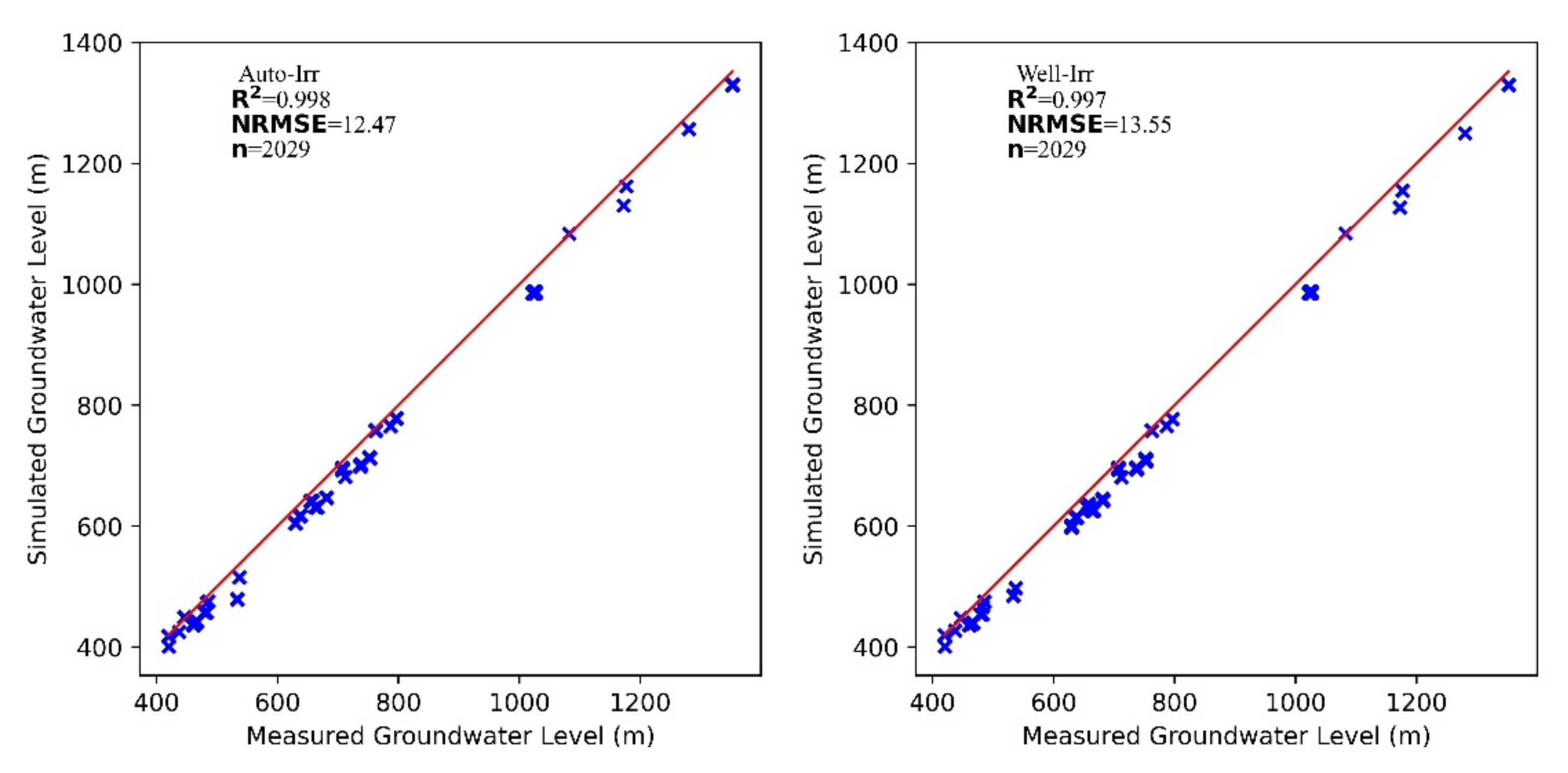
3.1.2. Groundwater Level
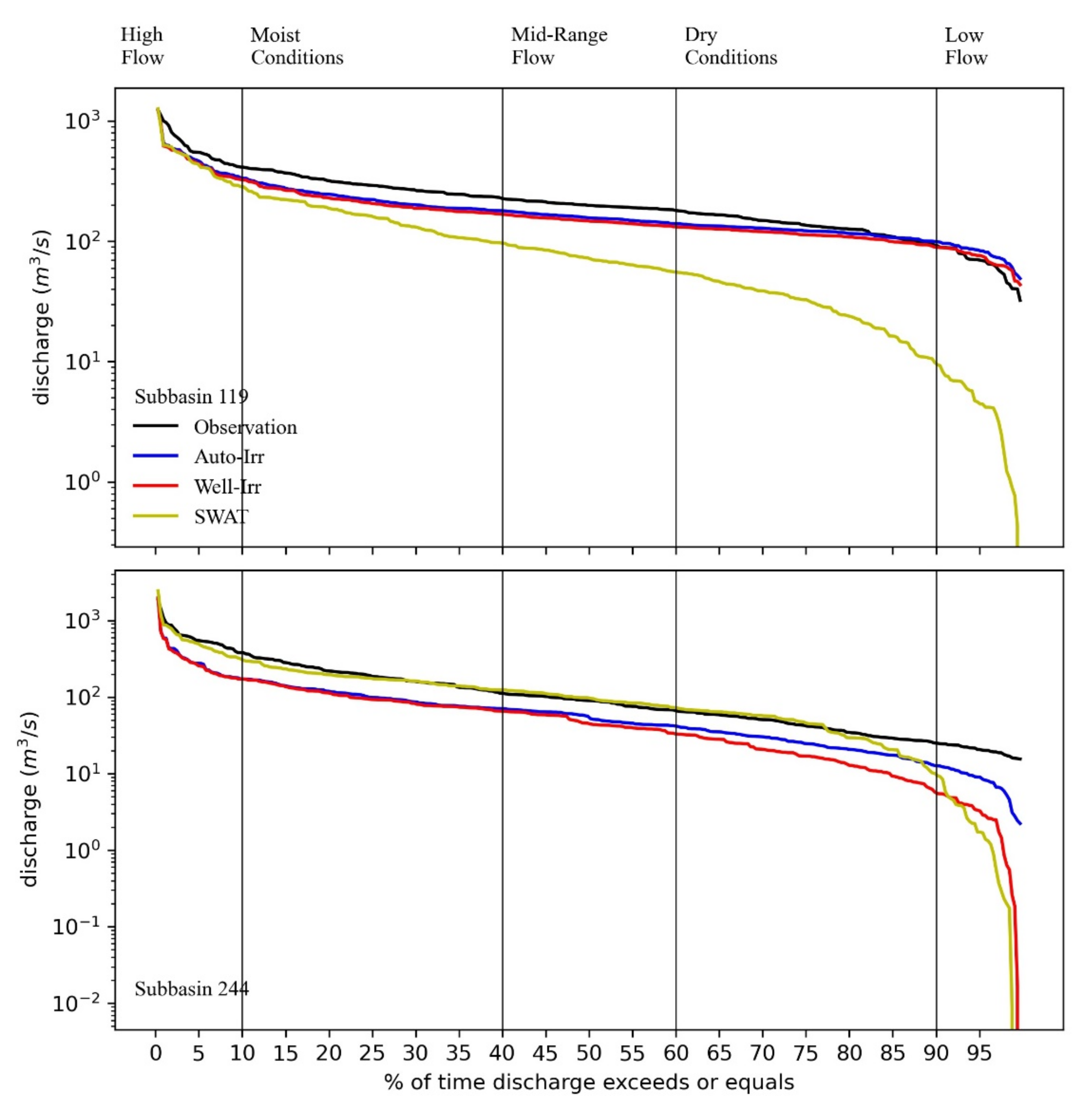
The monthly mean groundwater level simulated by the Auto-Irr and Well-Irr setups were compared with the observed monthly groundwater level from USGS as shown in Figure 4. The R2 for Auto-Irr and Well-Irr were found to be 0.998 and 0.997, respectively. This suggests that both irrigation settings were able to capture the dynamics of groundwater level variations. The NRMSE values also showed small differences between the two coupled model setups (13.55% (good) for Well-Irr, and 12.47% (good) for Auto-Irr). High hydraulic conductivity and specific yield across the NHP likely stabilized the saturated thickness of the aquifer despite large differences in groundwater withdrawals. However, for both setups, SWAT-MODFLOW underestimated the groundwater level compared with the observed values. The tendency of the model to simulate higher irrigation volumes (Figure 4) was a possible reason for model underestimation of the groundwater level. The mean bias error (MBE) and mean absolute error (MAE) for Auto-Irr were −25.5 m and 25.6 m, respectively. The corresponding values for the Well-Irr were −27.8 m and 27.8 m. In general, these errors were <3% of the mean measured groundwater levels. The model biases may have arisen from multiple reasons. For example, the mean elevation of the model grid cell of 1 km2 was different from the elevation of the USGS observation well, which was a single location in the cell. Errors may also have resulted from uncertainty in specifying model parameters, and pumping rates.

3.1.3. Streamflow

The Auto-Irr, Well-Irr and SWAT simulated streamflow were evaluated against the observed mean monthly streamflow data obtained from USGS gauges at the outlet corresponding to sub-basins 119 (northern) and 244 (southern) (Figure 1a). The model performance for three model setups is summarized in Table 2. More details about the time series of monthly mean simulated and observed streamflow at the outlet of sub-basins 119 and 244 are shown in Figure S2. For outlet 119, the R2 values were 0.66, 0.63 and 0.62 for SWAT, Auto-Irr and Well-Irr, respectively. All were greater than 0.5, suggesting that all model setups could capture the streamflow variation satisfactorily for the northern section of the NHP. The NSE values increased from 0.13 for the SWAT, to 0.55 and 0.51 for Auto-Irr and Well-Irr, respectively, in SWAT-MODFLOW. For outlet 244, SWAT outperformed SWAT-MODFLOW with Auto-Irr and Well-Irr setups in terms of both R2 and NSE. Auto-Irr slightly outperformed Well-Irr with an NSE of 0.53 vs. 0.51. Overall, at both locations, the SWAT-MODFLOW Auto-Irr (NSE = 0.53 and R2 = 0.6) simulation performed better than Well-Irr.
We further used flow duration curves (FDC) to better understand the model’s capability to simulate the streamflow regime. Figure 5 displays the streamflow regime (i.e., high flow to low flow conditions at outlets 119 and 244). Although the R2 and NSE values from the SWAT alone simulation at outlet 244 were greater than other coupled simulation results, it failed to capture the low flow regime at this site. The FDC analysis indicated that SWAT significantly underestimated the low flow regime at these two sites. The simplified representation of an aquifer in SWAT may have resulted in the rapid depletion of the aquifer water level when the aquifer was used as an irrigation source [76]. This could have reduced the baseflow and hence resulted in the underestimation of low flow regimes. Meanwhile, the low flow regime simulated by the coupled SWAT-MODFLOW setups were closer to the observed conditions when compared with SWAT. However, both SWAT-MODFLOW setups underestimated the high to mid-range flow regime for outlet 119. In the case of outlet 244, both SWAT-MODFLOW setups underestimated the entire flow regime. Among the coupled simulations, the largest underestimation of the low flow regime was found for Well-Irr. Overall, the performance of Auto-Irr for simulating stream discharge was the best among the coupled model setups. The SWAT-MODFLOW improved the R2 and NSE of streamflow in the northern section (i.e., sub-basin 119) of the NHP, demonstrating the positive influence of including a spatially variable groundwater system. In general, these results showed that SWAT-MODFLOW could simulate stream discharge at a large-scale watershed such as the NHP within the acceptable ranges based on model performance evaluation criteria.

3.1.4. Sub-Basin Evapotranspiration
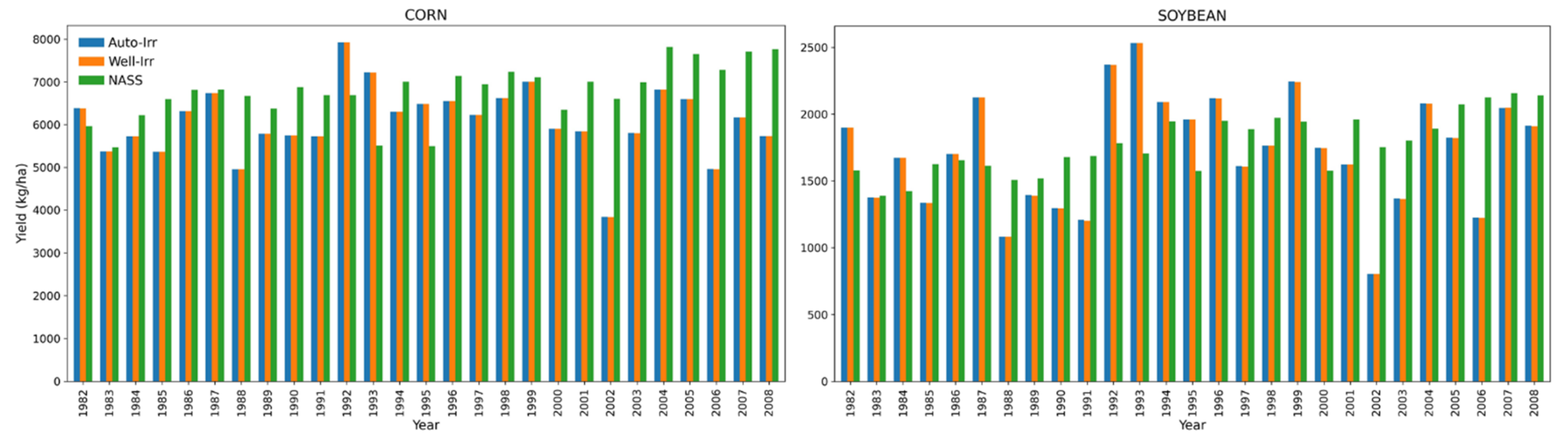
Figure 6a and Figure S3 show the Auto-Irr, Well-Irr and SWAT simulated mean annual ET for all the sub-basins in the NHP. The simulated monthly and annual ET in three model setups were similar. The model setup had negligible effects on ET. The simulated ET from Auto-Irr and MODIS ET (Figures S3 and S4) shows the spatial resemblance over the NHP with a west to east gradient, generally lower ET in western and northcentral sub-basins, and higher ET in the eastern sub-basins of the NHP (Figure 6a and Figure S4). The west–east gradient could be attributed to the west–east gradient in annual rainfall and irrigation distribution in the NHP. The average annual ET for the entire basin was found to be 512 mm and 376 mm for Auto-Irr and MODIS, respectively. The model estimated mean annual ET values for the NHP were 38% more than MODIS. The sub-basins with high ET in the east and south of the NHP coincided with the irrigated croplands which suggests that additional moisture from irrigation during the growing season facilitated the crop growth that could have contributed to higher ET in these regions.
The R2 of mean monthly ET at the sub-basin scale (Figure 6b) predicted by the Auto-Irr ranged from 0.01 to 0.80. The model simulated monthly ET with a mean R2 of 0.54 and more than 70% of sub-basins had an R2 greater than 0.5. Overall, the model performance indicated that the Auto-Irr with default SWAT parameters could provide reasonable estimates of monthly variation in ET at the sub-basin level.

3.1.5. Crop Yield

The NASS corn yield ranged from 5464 to 7820 kg/ha with an average of 6771 kg/ha, and the soybean yield ranged from 1389 to 2157 kg/ha with an average of 1774 kg/ha. The simulated corn yield shown in Figure 7 ranged from 3840 to 7927, and 3837 to 7925 kg/ha with an average of 6080 and 6078 kg/ha for Auto-Irr and Well-Irr, respectively. The simulated soybean yield ranged from 802 to 2533 kg/ha and 802 to 2532 kg/ha with an average of 1719 and 1717 kg/ha for Auto-Irr and Well-Irr, respectively. The small difference in simulated corn and soybean yield by Auto-Irr and Well-Irr showed that the crop yield was less sensitive to the choice of irrigation scheme. The overall PBIAS values for corn and soybean were 10.21 and 3.13% for Auto-Irr, and 10.23 and 3.21% for Well-Irr. This indicates good performance of the coupled model setups in simulating the corn and soybean yields.
Given that the monthly stream discharge, groundwater level, annual groundwater pumping volume and corn and soybean yield simulated by the Auto-Irr were comparable with the observed values, and that the performance statistics indicated that the model could provide a reasonable characterization of the regional hydrological processes, Auto-Irr was used to assess the impact of water management practices in the NHP.

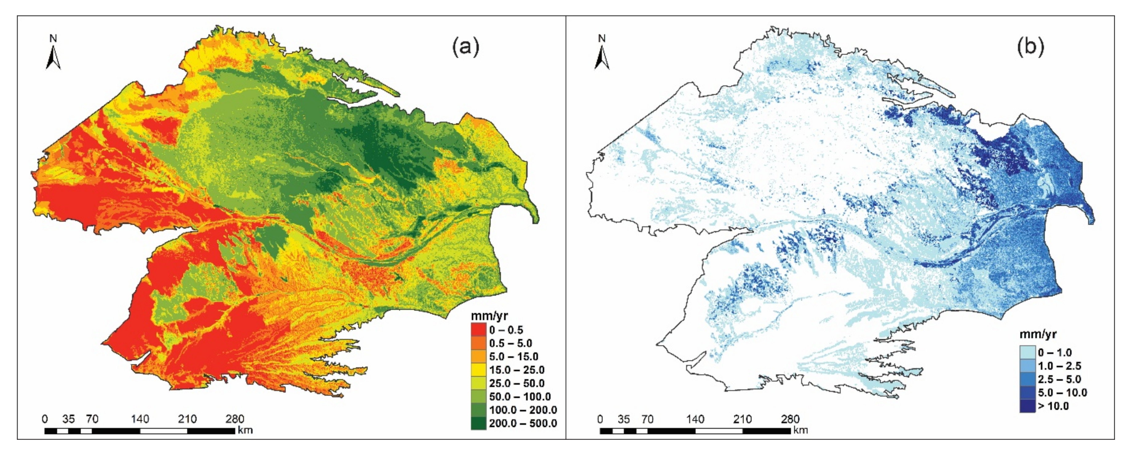
3.2. Irrigation Impacts on Groundwater Recharge

Groundwater recharge can be spatially variable depending on the vegetation, soil type and climate. First, groundwater recharge over the NHP was examined under the current land and water management practices and then compared with a “no-irrigation” scenario to understand the overall impact of irrigation on groundwater recharge.
The spatial distribution of the long term (1982–2008) mean annual recharge rate is displayed in Figure 8a. The mean annual recharge averaged across the NHP aquifer was 48.01 mm yr−1, close to the value of 48 mm yr−1 obtained by [77], a regional recharge study for Nebraska based on a simple water balance method. It was spatially variable with significant recharge around the north-central NHP (Sand Hills) and along the Platte and Elkhorn rivers. The recharge rate reached as high as 500 mm yr−1 in the Sand Hills and less than 0.5 mm yr−1 over the southern NHP and west of Sand Hills where precipitation is minimal and where the aquifer consists of clay soils. The elevated recharge rates in the northern part relative to the south of the NHP was associated with the soil properties which follow a gradient of high permeability in the north, to low permeability in the south [12]. The highly permeable sandy soils in Sand Hills reduce evapotranspiration and promote infiltration [78]. The combination of low evapotranspiration and high infiltration rates over Sand Hills could explain the higher groundwater recharge rate. The spatial pattern of recharge was consistent with previously published studies [12,77,79]. A study by Zhang et al. [79] used the Soil Water Balance (SWB) model to estimate the mean annual recharge for the period of 1950–2010 in the NHP that ranged from 0 to 499 mm yr−1, matching closely with the 0–500 mm yr−1 range estimated in this study.
The spatial distribution of the difference in precipitation and ET (P-ET) in Figure 9a illustrates negative P-ET terms in the western and southern sub-basins. These sub-basins mostly corresponded with the areas of high irrigation demand dominated by irrigated crops (Figure 9b–d), low precipitation (Figure S1) and low permeability of soils, which contributed to negligible recharge ~0 mm yr−1 (Figure 8a) despite additional water from irrigation in the region. Meanwhile, we found that in the eastern part of the NHP which receives high precipitation, despite high irrigation demand, mean annual precipitation exceeded the mean annual ET, resulting in a relatively higher recharge rate in the eastern NHP than the western and southern parts (Figure 8a). Our result was supported by the similar findings of Crosbie et al. [80], that identified the high recharge rate in eastern Nebraska which was linked with the irrigation and coarse-textured soils.
Upon comparing the Auto-Irr and “no irrigation” scenarios from Figure 8b, we found that the regions with increased recharge overlapped the areas with irrigation wells. In irrigated areas, irrigation resulted in an overall increase in annual recharge that could exceed 10 mm yr−1. The high recharge rates (>5 mm yr−1) as a result of irrigation were found along the Platte and Elkhorn rivers. The groundwater recharge change due to irrigation was relatively small (~3.6%) in the study region. The previous studies that evaluated the effect of irrigation on groundwater recharge within our study region reported similar results. A study by Zhang et al. [79] also found the negligible impact of irrigation on groundwater recharge in the NHP.

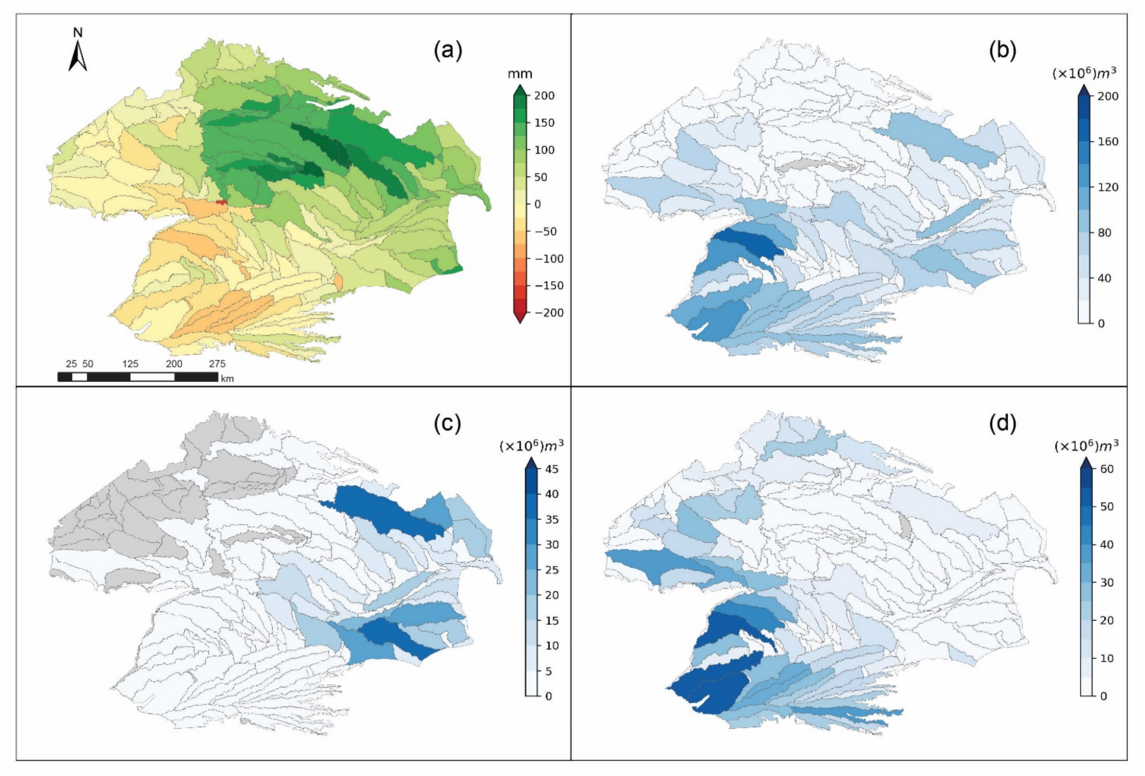
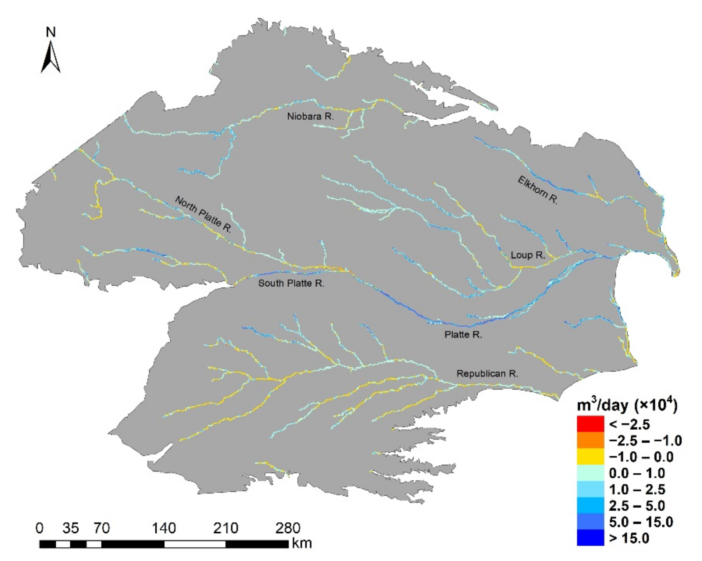
3.3. Irrigation Impacts on Surface-Groundwater Exchange

A comparison of the change in surface and groundwater exchange indicated that intensive irrigation could have a significant influence on the river discharge. In the absence of irrigation, on average there was an increase in groundwater discharge to all of the major rivers (Figure 10). Comparing the long-term annual average surface–groundwater exchange rates between irrigated and non-irrigated scenarios (Table 3) shows that irrigation practices decreased the groundwater discharge by 1.60 to 9.66 m3/s. The greatest decrease of 9.66 m3/s was found in the Platte River, followed by the Loup, Elkhorn, South Platte, Republican, Niobara, and North Platte rivers. These results indicated the significant effect of intensive irrigation on surface-groundwater exchange in the NHP, in good agreement with the Kustu et al. [13] finding that stream discharge was highly sensitive to irrigation pumping.

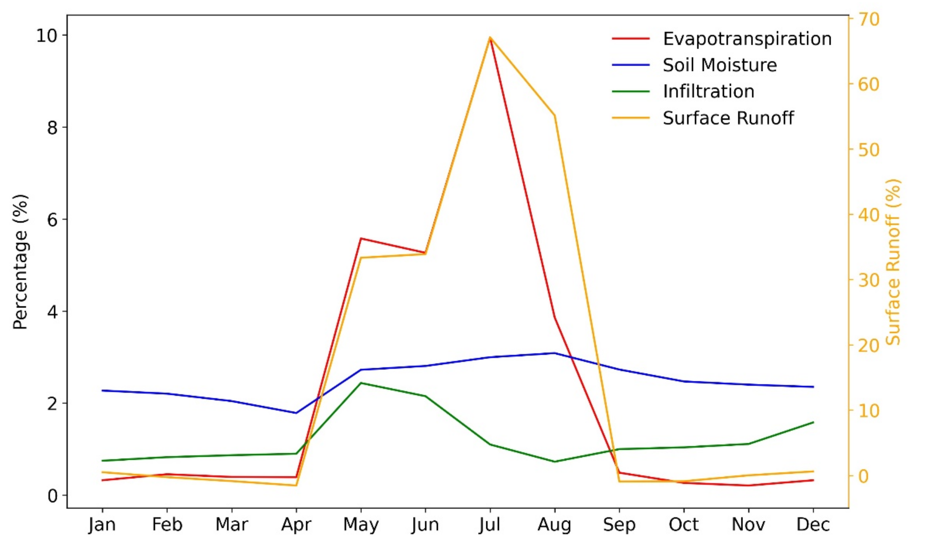
3.4. Hydrological Responses to Irrigation

A comparison of the effects of irrigation on the watershed scale water budget components (streamflow, groundwater recharge and evapotranspiration) relative to the no-irrigation scenario over 1982–2008 for sub-basins overlaying the NHP aquifer is shown in Figure 11. The intensive irrigation in the region resulted in the largest impact on surface runoff (particularly during the growing season) and altered other water budget components. On the annual scale, as a result of irrigation, surface runoff increased 21.3%, groundwater infiltration increased 1.5%, soil water content increased 2.5% and ET increased 4.0%, compared with the no-irrigation scenario. It can be inferred that additional water from irrigation slightly increased soil water content and infiltration, resulting in more groundwater recharge and evapotranspiration, as well as higher surface runoff. The significant increase in seasonal surface runoff (up to 67% in July) demonstrates the potential impacts on the aquatic ecological system in the NHP caused by intensive irrigation.

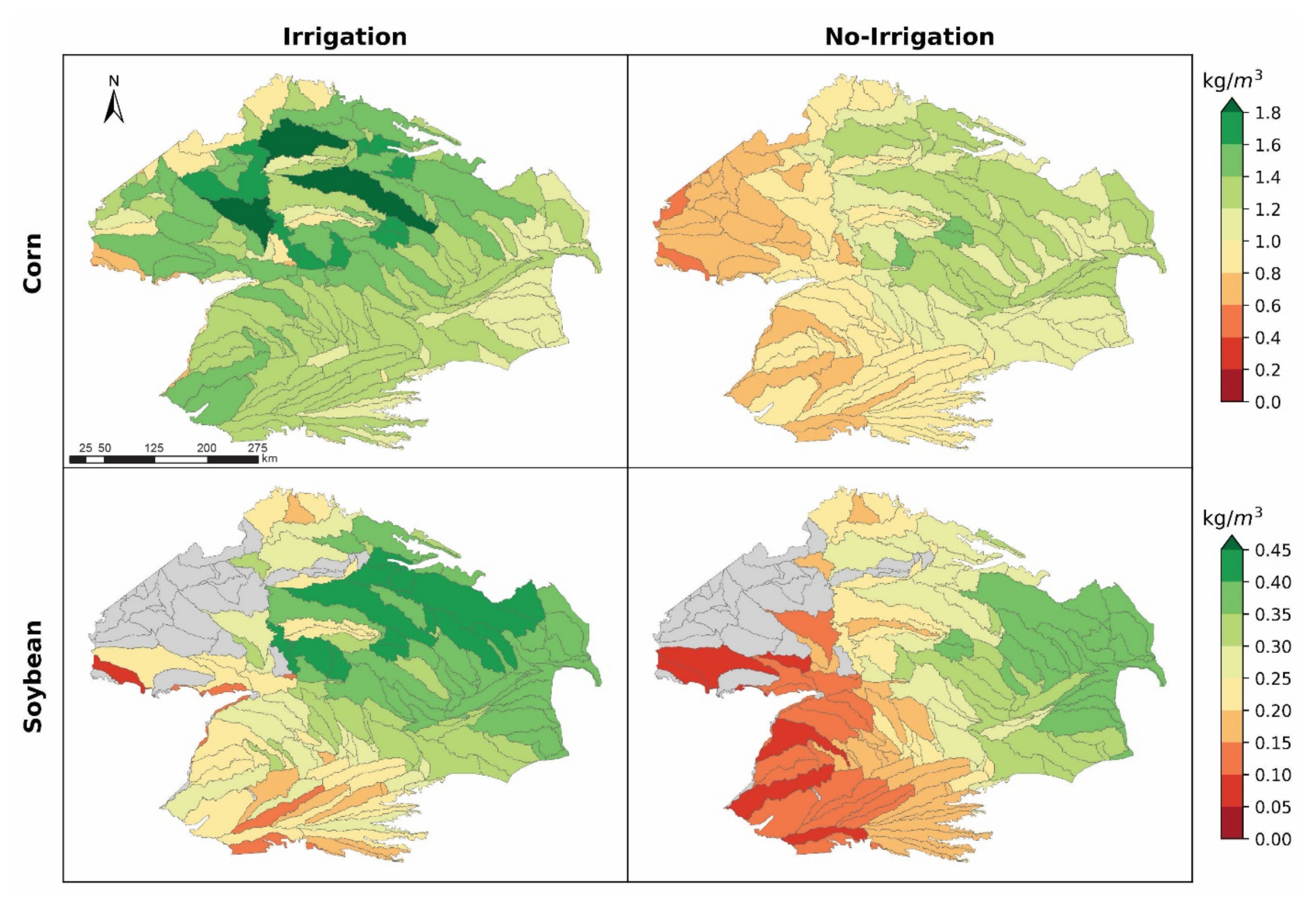
3.5. Irrigation Impacts on Crop Water Productivity

Figure 12 shows the changes in the average CWP (1982–2008) of corn and soybean, respectively, for the irrigation and no-irrigation scenarios. In the absence of irrigation, the CWP (corn and soybean) showed an upward west–east gradient, with lower values in the west and higher values in the east, which correlated with the precipitation distribution in the region (Figure S1). This illustrates that the drier climate in the western sub-basins limited the crop yield. The simulated CWP for corn and soybean ranged from 0.39–1.8, and 0.01–0.39 kg/m3, respectively. With irrigation, the average CWP of corn and soybean increased by 27.2 and 23.8%, respectively, at the sub-basin level. Correspondingly, the simulated irrigated CWP for corn and soybean ranged from 0.39–1.9, and 0.01–0.44 kg/m3, respectively. Note that, the CWP increase in the eastern sub-basins under the irrigation scenario was minimal or closer to the no-irrigation scenario. The minimal CWP increase in the east of the NHP was not a surprise as the water deficit under no-irrigation was minimal. Meanwhile, in the western and central sub-basins where the water deficit was large, we observed pronounced increases in CWP, which suggested that the additional water from irrigation significantly increased the crop yield in those dry regions.

4. Discussions

Caution should be used when interpreting the results from this study, which are subject to multiple caveats. For example, our model configuration assumes constant land use and land cover throughout the simulation period that presents difficulty in an accurate estimation of the irrigation demand and recharge rates. Additionally, the canal seepage was not simulated, which adds to the uncertainty in the modeled recharge rates. Therefore, further studies to allow dynamic land-use change and better representation of canal irrigation systems are needed.
Note that in our model evaluation and application, we did not apply automatic parameter calibration algorithms to adjust numerous parameters within the model. We made this choice for two reasons. First, the SWAT model was originally developed to operate in large-scale ungauged watersheds with minimal calibration efforts [81], and Zhang et al. [82] and Arnold et al. [83] noted that parameter calibration in many cases could not guarantee high fidelity of modeling results. Second, automatic optimization algorithms often require a large amount of resources and long times to identify globally optimal parameter solutions for complex hydrologic models such as SWAT [84], which is currently not affordable, as running SWAT-MODFLOW once for the NHP takes multiple days. As such, to ensure an objective comparison between different models, we used default model parameters or derived parameters from literature instead of intensively calibrating numerous parameters of SWAT-MODFLOW. In the future, further modifications of SWAT-MODFLOW are needed to assess the applicability of parallel processing for drastically reducing the computational resources needed to run the coupled model, thereby allowing for numerous model runs and understanding uncertainties associated with parameters and input data.

5. Summary and Conclusions

In this study, we conducted modification and evaluation of the SWAT-MODFLOW model’s irrigation modules for improved representation of irrigation practices and the exchange of water fluxes in the U.S. Northern High Plains (NHP) aquifer. We found that SWAT-MODFLOW with irrigation based on auto-irrigation scheduling, triggered by plant water stress (Auto-Irr), attained better performance than SWAT-MODFLOW with prescribed irrigation based on well pumping rates in MODFLOW (Well-Irr) in terms of groundwater level, streamflow, and ET, and was capable of explicitly representing groundwater level change as compared with the original SWAT model. Therefore, Auto-Irr was used to quantify and understand hydrologic and agronomic impacts of the intensive irrigation practices in the NHP.
The results showed that the groundwater recharge rate and groundwater level changes in the NHP were spatially variable and were all substantially impacted by irrigation practices. A comparison of Auto-Irr results with “no-irrigation” scenarios showed that intensive irrigation in the region had a significant impact on the groundwater levels and crop water productivity, but only exerted a modest effect on groundwater recharge, except in the region with dense irrigation wells.
The irrigation-caused changes in groundwater systems also translated into alterations in other hydrological processes, including streamflow, evapotranspiration (ET), soil moisture and groundwater recharge. In general, the impact of irrigation slightly altered soil moisture, and groundwater recharge, but significantly modified ET and streamflow regimes in the NHP, particularly during the growing season. For example, on the annual scale, as a result of irrigation, ET and surface runoff increased by 4.0% and 21.3%, respectively. During July, irrigation practices increased ET by 9.9% and surface runoff by 67.1%. Such large changes in surface runoff resulting from irrigation are expected to have significant impacts on aquatic ecosystems, which deserves further research in the future. Irrigation in the NHP also significantly increased corn and soybean yields and their crop water productivity (CPW). With irrigation, the average CWP of corn and soybean increased by 27.2 and 23.8%.
Overall, historical irrigation in the NHP greatly benefited crop productivity, and caused pronounced modifications to the groundwater systems and other hydrological processes. Particularly, the decline in groundwater level raises concerns for future sustainable irrigation in the face of a warming climate; and significant alterations in streamflow during the growing season indicates that future design of sustainable irrigation practices should consider downstream aquatic ecosystems impacts. We anticipate that the exercises conducted here help to increase the understanding of the hydrological and agronomic impacts of historical irrigation, and provide support for future efforts to enhance agroecosystem sustainability in the NHP and other regions facing water shortage challenges.

Supplementary Materials

The following supporting information can be downloaded at: https://www.mdpi.com/article/10.3390/w14121938/s1, Figure S1: North American Regional Reanalysis (NARR) based average annual precipitation (1982–2008) at the sub-basin scale for SWAT domain; Figure S2: Monthly mean streamflow at the outlet of watersheds in Northern High Plains; Figure S3: Sub-basin level mean annual evapotranspiration simulated by (a) SWAT only, and (b) Well-Irr, for 2000–2008; Figure S4: Sub-basin level mean annual evapotranspiration estimated from Moderate Resolution Imaging Spectroradiometer (MODIS) from 2000–2008; Table S1: Reservoir summary.

Author Contributions

Conceptualization, X.Z., F.M.-W., X.-Z.L. and S.D.; methodology, S.D.; software, S.D.; validation, S.D.; formal analysis, S.D.; investigation, S.D.; resources, X.Z., F.M.-W., X.-Z.L.; data curation, X.Z., F.M.-W.; writing—original draft preparation, S.D.; writing—review and editing, S.D., X.Z., F.M.-W. and X.-Z.L.; visualization, S.D.; supervision, F.M.-W., X.Z., X.-Z.L.; project administration, X.Z., F.M.-W., X.-Z.L.; funding acquisition, X.-Z.L., F.M.-W. All authors have read and agreed to the published version of the manuscript.

Funding

The research was supported by the National Science Foundation Innovations at the Nexus of Food, Energy and Water Systems under grants EAR-1639327 and EAR-1903249, and National Research Traineeship Program NRT-INFEWS: UMD Global STEWARDS (STEM Training at the Nexus of Energy, Water Reuse and Food Systems) under grant 1828910. This research was supported in part by the U.S. Department of Agriculture, Agricultural Research Service. USDA is an equal opportunity provider and employer.

Data Availability Statement

The data presented in this study are available on request from the corresponding author.

Conflicts of Interest

The authors declare no conflict of interest.

References

  1. Carruthers, I.; Rosegrant, M.W.; Seckler, D. Irrigation and Food Security in the 21st Century. Irrig. Drain. Syst. 1997, 11, 83–101. [Google Scholar] [CrossRef]
  2. FAO. The State of the World’s Land and Water Resources for Food and Agriculture: Managing Systems at Risk; Food and Agriculture Organization: Rome, Italy; Earthscan: London, UK, 2011. [Google Scholar]
  3. Rost, S.; Gerten, D.; Bondeau, A.; Lucht, W.; Rohwer, J.; Schaphoff, S. Agricultural Green and Blue Water Consumption and Its Influence on the Global Water System. Water Resour. Res. 2008, 44, W09405. [Google Scholar] [CrossRef] [Green Version]
  4. Garces-Restrepo, C.; Vermillion, D.; Muñoz, G. Irrigation Management Transfer. Worldwide Efforts and Results; FAO Water Reports 32; International Irrigation Management Institute, FAO: Rome, Italy, 2007; 62p. [Google Scholar]
  5. Colaizzi, P.D.; Gowda, P.H.; Marek, T.H.; Porter, D.O. Irrigation in the Texas High Plains: A Brief History and Potential Reductions in Demand. Irrig. Drain. J. Int. Comm. Irrig. Drain. 2009, 58, 257–274. [Google Scholar] [CrossRef]
  6. Aldaya, M.M.; Allan, J.A.; Hoekstra, A.Y. Strategic Importance of Green Water in International Crop Trade. Ecol. Econ. 2010, 69, 887–894. [Google Scholar] [CrossRef] [Green Version]
  7. Maupin, M.A.; Barber, N.L. Estimated Withdrawals from Principal Aquifers in the United States, 2000; US Geological Survey Circular: Reston, VA, USA, 2005; pp. 1–51. [CrossRef] [Green Version]
  8. Scanlon, B.R.; Faunt, C.C.; Longuevergne, L.; Reedy, R.C.; Alley, W.M.; McGuire, V.L.; McMahon, P.B. Groundwater Depletion and Sustainability of Irrigation in the US High Plains and Central Valley. Proc. Natl. Acad. Sci. USA 2012, 109, 9320–9325. [Google Scholar] [CrossRef] [PubMed] [Green Version]
  9. Barlow, P.M.; Leake, S.A. Streamflow Depletion by Wells: Understanding and Managing the Effects of Groundwater Pumping on Streamflow; US Geological Survey Circular: Reston, VA, USA, 2012.
  10. Wen, F.; Chen, X. Evaluation of the Impact of Groundwater Irrigation on Streamflow in Nebraska. J. Hydrol. 2006, 327, 603–617. [Google Scholar] [CrossRef]
  11. Haacker, E.M.K.; Kendall, A.D.; Hyndman, D.W. Water Level Declines in the High Plains Aquifer: Predevelopment to Resource Senescence. Groundwater 2016, 54, 231–242. [Google Scholar] [CrossRef]
  12. Smidt, S.J.; Haacker, E.M.K.; Kendall, A.D.; Deines, J.M.; Pei, L.; Cotterman, K.A.; Li, H.; Liu, X.; Basso, B.; Hyndman, D.W. Complex Water Management in Modern Agriculture: Trends in the Water-Energy-Food Nexus over the High Plains Aquifer. Sci. Total Environ. 2016, 566–567, 988–1001. [Google Scholar] [CrossRef] [Green Version]
  13. Kustu, M.D.; Fan, Y.; Robock, A. Large-Scale Water Cycle Perturbation Due to Irrigation Pumping in the US High Plains: A Synthesis of Observed Streamflow Changes. J. Hydrol. 2010, 390, 222–244. [Google Scholar] [CrossRef]
  14. Nebraska Department of Natural Resources (NDNR). 2017 Annual Evaluation of Availability of Hydrologically Connected Water Supplies; NDNR: Lincoln, NE, USA, 2016; p. 165. [Google Scholar]
  15. Hua, L.; Wang, H.; Sui, H.; Wardlow, B.; Hayes, M.J.; Wang, J. Mapping the Spatial-Temporal Dynamics of Vegetation Response Lag to Drought in a Semi-Arid Region. Remote Sens. 2019, 11, 1873. [Google Scholar] [CrossRef] [Green Version]
  16. Zhang, J.; Campana, P.E.; Yao, T.; Zhang, Y.; Lundblad, A.; Melton, F.; Yan, J. The Water-Food-Energy Nexus Optimization Approach to Combat Agricultural Drought: A Case Study in the United States. Appl. Energy 2018, 227, 449–464. [Google Scholar] [CrossRef]
  17. Bathke, D.J.; Oglesby, R.J.; Rowe, C.; Wilhite, D.A. Understanding and Assessing Climate Change: Implications for Nebraska; University of Nebraska-Lincoln: Lincoln, NE, USA, 2014. [Google Scholar]
  18. Gao, L.; Li, D. A Review of Hydrological/Water-Quality Models. Front. Agric. Sci. Eng. 2014, 1, 267–276. [Google Scholar] [CrossRef] [Green Version]
  19. Daggupati, P.; Deb, D.; Srinivasan, R.; Yeganantham, D.; Mehta, V.M.; Rosenberg, N.J. Large-Scale Fine-Resolution Hydrological Modeling Using Parameter Regionalization in the Missouri River Basin. JAWRA J. Am. Water Resour. Assoc. 2016, 52, 648–666. [Google Scholar] [CrossRef]
  20. Peterson, S.M.; Flynn, A.T.; Traylor, J.P. Groundwater-Flow Model of the Northern High Plains Aquifer in Colorado, Kansas, Nebraska, South Dakota, and Wyoming; Scientific Investigations Report; US Geological Survey: Reston, VA, USA, 2016; p. 102.
  21. Rossman, N.R.; Zlotnik, V.A.; Rowe, C.M. An Approach to Hydrogeological Modeling of a Large System of Groundwater-Fed Lakes and Wetlands in the Nebraska Sand Hills, USA. Hydrogeol. J. 2018, 26, 881–897. [Google Scholar] [CrossRef] [Green Version]
  22. Strauch, K.R.; Linard, J.I. Streamflow Simulations and Percolation Estimates Using the Soil and Water Assessment Tool for Selected Basins in North-Central Nebraska, 1940–2005; Scientific Investigations Report 2009–5075; US Geological Survey: Reston, VA, USA, 2009; p. 20.
  23. Zeng, R.; Cai, X. Analyzing Streamflow Changes: Irrigation-Enhanced Interaction between Aquifer and Streamflow in the Republican River Basin. Hydrol. Earth Syst. Sci. 2014, 18, 493–502. [Google Scholar] [CrossRef] [Green Version]
  24. Srinivasan, R.; Zhang, X.; Arnold, J. SWAT Ungauged: Hydrological Budget and Crop Yield Predictions in the Upper Mississippi River Basin. Trans. ASABE 2010, 53, 1533–1546. [Google Scholar] [CrossRef]
  25. Chen, X.; Chen, X. Simulating the Effects of Reduced Precipitation on Ground Water and Streamflow in the Nebraska Sand Hills. JAWRA J. Am. Water Resour. Assoc. 2004, 40, 419–430. [Google Scholar] [CrossRef]
  26. Hrozencik, R.A.; Manning, D.T.; Suter, J.F.; Goemans, C.; Bailey, R.T. The Heterogeneous Impacts of Groundwater Management Policies in the Republican River Basin of Colorado. Water Resour. Res. 2017, 53, 10757–10778. [Google Scholar] [CrossRef] [Green Version]
  27. Bailey, R.T.; Wible, T.C.; Arabi, M.; Records, R.M.; Ditty, J. Assessing Regional-Scale Spatio-Temporal Patterns of Groundwater—Surface Water Interactions Using a Coupled SWAT-MODFLOW Model. Hydrol. Process. 2016, 30, 4420–4433. [Google Scholar] [CrossRef]
  28. Molina-Navarro, E.; Bailey, R.T.; Andersen, H.E.; Thodsen, H.; Nielsen, A.; Park, S.; Jensen, J.S.; Jensen, J.B.; Trolle, D. Comparison of Abstraction Scenarios Simulated by SWAT and SWAT-MODFLOW. Hydrol. Sci. J. 2019, 64, 434–454. [Google Scholar] [CrossRef]
  29. Frederiksen, R.R.; Molina-Navarro, E. The Importance of Subsurface Drainage on Model Performance and Water Balance in an Agricultural Catchment Using SWAT and SWAT-MODFLOW. Agric. Water Manag. 2021, 255, 107058. [Google Scholar] [CrossRef]
  30. Kollet, S.J.; Maxwell, R.M. Integrated Surface–Groundwater Flow Modeling: A Free-Surface Overland Flow Boundary Condition in a Parallel Groundwater Flow Model. Adv. Water Resour. 2006, 29, 945–958. [Google Scholar] [CrossRef] [Green Version]
  31. Sutanudjaja, E.H.; van Beek, L.P.H.; de Jong, S.M.; van Geer, F.C.; Bierkens, M.F.P. Large-Scale Groundwater Modeling Using Global Datasets: A Test Case for the Rhine-Meuse Basin. Hydrol. Earth Syst. Sci. 2011, 15, 2913–2935. [Google Scholar] [CrossRef] [Green Version]
  32. Markstrom, S.L.; Niswonger, R.G.; Regan, R.S.; Prudic, D.E.; Barlow, P.M. GSFLOW—Coupled Groundwater and Surface-Water Flow Model Based on the Integration of the Precipitation-Runoff Modeling System (PRMS) and the Modular Ground-Water Flow Model (MODFLOW-2005); U.S. Geological Survey Techniques and Methods 6-D1; U.S. Geological Survey: Reston, VA, USA, 2008; p. 254.
  33. Kim, N.W.; Chung, I.M.; Won, Y.S.; Arnold, J.G. Development and Application of the Integrated SWAT–MODFLOW Model. J. Hydrol. 2008, 356, 1–16. [Google Scholar] [CrossRef]
  34. Sophocleous, M.A.; Koelliker, J.K.; Govindaraju, R.S.; Birdie, T.; Ramireddygari, S.R.; Perkins, S.P. Integrated Numerical Modeling for Basin-Wide Water Management: The Case of the Rattlesnake Creek Basin in South-Central Kansas. J. Hydrol. 1999, 214, 179–196. [Google Scholar] [CrossRef]
  35. Jin, X.; Jin, Y.; Mao, X.; Zhai, J.; Fu, D. Modelling the Impact of Vegetation Change on Hydrological Processes in Bayin River Basin, Northwest China. Water 2021, 13, 2787. [Google Scholar] [CrossRef]
  36. Chunn, D.; Faramarzi, M.; Smerdon, B.; Alessi, D. Application of an Integrated SWAT–MODFLOW Model to Evaluate Potential Impacts of Climate Change and Water Withdrawals on Groundwater–Surface Water Interactions in West-Central Alberta. Water 2019, 11, 110. [Google Scholar] [CrossRef] [Green Version]
  37. Liu, W.; Bailey, R.T.; Andersen, H.E.; Jeppesen, E.; Nielsen, A.; Peng, K.; Molina-Navarro, E.; Park, S.; Thodsen, H.; Trolle, D. Quantifying the Effects of Climate Change on Hydrological Regime and Stream Biota in a Groundwater-Dominated Catchment: A Modelling Approach Combining SWAT-MODFLOW with Flow-Biota Empirical Models. Sci. Total Environ. 2020, 745, 140933. [Google Scholar] [CrossRef]
  38. Aliyari, F.; Bailey, R.T.; Tasdighi, A.; Dozier, A.; Arabi, M.; Zeiler, K. Coupled SWAT-MODFLOW Model for Large-Scale Mixed Agro-Urban River Basins. Environ. Model. Softw. 2019, 115, 200–210. [Google Scholar] [CrossRef]
  39. Wei, X.; Bailey, R.T. Assessment of System Responses in Intensively Irrigated Stream-Aquifer Systems Using SWAT-MODFLOW. Water 2019, 11, 1576. [Google Scholar] [CrossRef] [Green Version]
  40. Liu, W.; Park, S.; Bailey, R.T.; Molina-Navarro, E.; Andersen, H.E.; Thodsen, H.; Nielsen, A.; Jeppesen, E.; Jensen, J.S.; Jensen, J.B.; et al. Comparing SWAT with SWAT-MODFLOW Hydrological Simulations When Assessing the Impacts of Groundwater Abstractions for Irrigation and Drinking Water. Hydrol. Earth Syst. Sci. Discuss. 2019, 1–51. [Google Scholar] [CrossRef] [Green Version]
  41. Bailey, R.T.; Park, S. SWAT-MODFLOW Tutorial Version3—Documentation for Preparing and Running SWAT-MODFLOW Simulations; Department of Civil and Environmental Engineering, Colorado State University: Fort Collins, CO, USA, 2019. [Google Scholar]
  42. Chen, Y.; Marek, G.W.; Marek, T.H.; Brauer, D.K.; Srinivasan, R. Assessing the Efficacy of the SWAT Auto-Irrigation Function to Simulate Irrigation, Evapotranspiration, and Crop Response to Management Strategies of the Texas High Plains. Water 2017, 9, 509. [Google Scholar] [CrossRef]
  43. Klocke, N.L.; Hubbard, K.; Kranz, W.L.; Watts, D.G. G90-992 Evapotranspiration (ET) or Crop Water Use; Historical Materials from University of Nebraska-Lincoln Extension; University of Nebraska-Lincoln Extension Division: Lincoln, NE, USA, 1990; p. 1197. [Google Scholar]
  44. Hutson, S.S.; Barber, N.L.; Kenny, J.F.; Linsey, K.S.; Lumia, D.S.; Maupin, M.A. Estimated Use of Water in the United States in 2000; Revised Fe.; Circular: Reston, VA, USA, 2004. [Google Scholar]
  45. Dieter, C.A.; Maupin, M.A.; Caldwell, R.R.; Harris, M.A.; Ivahnenko, T.I.; Lovelace, J.K.; Barber, N.L.; Linsey, K.S. Estimated Use of Water in the United States in 2015; Circular: Reston, VA, USA, 2018; p. 76. [Google Scholar]
  46. Neitsch, S.L.; Arnold, J.G.; Kiniry, J.R.; Williams, J.R. Soil and Water Assessment Tool Theoretical Documentation Version 2009; Texas Water Resources Institute: College Station, TX, USA, 2011; p. 647. [Google Scholar]
  47. Douglas-Mankin, K.R.; Srinivasan, R.; Arnold, J.G. Soil and Water Assessment Tool (SWAT) Model: Current Developments and Applications. Trans. ASABE 2010, 53, 1423–1431. [Google Scholar] [CrossRef]
  48. Garg, K.K.; Bharati, L.; Gaur, A.; George, B.; Acharya, S.; Jella, K.; Narasimhan, B. Spatial Mapping of Agricultural Water Productivity Using the SWAT Model in Upper Bhima Catchment, India. Irrig. Drain. 2012, 61, 60–79. [Google Scholar] [CrossRef] [Green Version]
  49. USDA NASS. Cropland Data Layer Published Crop-Specific Data Layer [Online]; USDA-NASS: Washington, DC, USA, 2008; Available online: https://nassgeodata.gmu.edu/cropscape/ (accessed on 28 March 2019).
  50. Pervez, M.S.; Brown, J.F. Mapping Irrigated Lands at 250-m Scale by Merging MODIS Data and National Agricultural Statistics. Remote Sens. 2010, 2, 2388–2412. [Google Scholar] [CrossRef] [Green Version]
  51. Woznicki, S.A.; Nejadhashemi, A.P. Sensitivity Analysis of Best Management Practices under Climate Change Scenarios 1: Sensitivity Analysis of Best Management Practices under Climate Change Scenarios. JAWRA J. Am. Water Resour. Assoc. 2012, 48, 90–112. [Google Scholar] [CrossRef]
  52. Ferguson, R.B.; Shapiro, C.A.; Dobermann, A.R.; Wortmann, C.S. G87-859 Fertilizer Recommendations for Soybean (Revised August 2006); Historical Materials from University of Nebraska-Lincoln Extension; University of Nebraska-Lincoln Extension Division: Lincoln, NE, USA, 2006. [Google Scholar]
  53. Van Liew, M.W.; Feng, S.; Pathak, T.B. Climate Change Impacts on Streamflow, Water Quality, and Best Management Practices for the Shell and Logan Creek Watersheds in Nebraska, USA. Int. J. Agric. Biol. Eng. 2012, 5, 13–34. [Google Scholar] [CrossRef]
  54. Mesinger, F.; DiMego, G.; Kalnay, E.; Mitchell, K.; Shafran, P.C.; Ebisuzaki, W.; Jović, D.; Woollen, J.; Rogers, E.; Berbery, E.H.; et al. North American Regional Reanalysis. Bull. Am. Meteorol. Soc. 2006, 87, 343–360. [Google Scholar] [CrossRef] [Green Version]
  55. Jarvis, A.; Reuter, H.I.; Nelson, A.; Guevara, E. Hole-Filled SRTM for the Globe Version 4. The CGIAR-CSI SRTM 90 m Database. 2008. Available online: http://srtm.csi.cgiar.org (accessed on 17 October 2017).
  56. USDA-NRCS. State Soil Geographic (STATSGO) Database—Data User Guide; U.S. Department of Agriculture, Natural Resources Conservation Service, Miscellaneous Publication: Washington, DC, USA, 1994.
  57. United States Bureau of Reclamation, (USBR) Hydromet. 2019. Available online: https://Www.Usbr.Gov/Pn/Hydromet/ (accessed on 5 March 2019).
  58. US Army Corps of Engineers. Annual Report of Reservoir Regulation Activities: Summary for 2011–2012; US Army Corps of Engineers, Kansas City District, Engineering Division, Hydrologic Engineering Branch, Water Management Section; USACE: Washington, DC, USA, 2013.
  59. Essou, G.R.C.; Sabarly, F.; Lucas-Picher, P.; Brissette, F.; Poulin, A. Can Precipitation and Temperature from Meteorological Reanalyses Be Used for Hydrological Modeling? J. Hydrometeorol. 2016, 17, 1929–1950. [Google Scholar] [CrossRef]
  60. Harbaugh, A.W. MODFLOW-2005, The U.S. Geological Survey Modular Ground-Water Model—The Ground-Water Flow Process: U.S. Geological Survey Techniques and Methods 6-A16; Modeling Techniques; U.S. Geological Survey: Reston, VA, USA, 2005.
  61. Nebraska Department of Natural Resources. Groundwater Wells Database; Nebraska Department of Natural Resources: Lincoln, NE, USA, 2020. [Google Scholar]
  62. Marek, G.W.; Gowda, P.H.; Marek, T.H.; Porter, D.O.; Baumhardt, R.L.; Brauer, D.K. Modeling Long-Term Water Use of Irrigated Cropping Rotations in the Texas High Plains Using SWAT. Irrig. Sci. 2017, 35, 111–123. [Google Scholar] [CrossRef]
  63. Chen, X. Streambed Hydraulic Conductivity for Rivers in South-Central Nebraska. JAWRA J. Am. Water Resour. Assoc. 2004, 40, 561–573. [Google Scholar] [CrossRef]
  64. Cheng, C.; Song, J.; Chen, X.; Wang, D. Statistical Distribution of Streambed Vertical Hydraulic Conductivity along the Platte River, Nebraska. Water Resour. Manag. 2011, 25, 265–285. [Google Scholar] [CrossRef] [Green Version]
  65. Song, J.X.; Chen, X.H.; Cheng, C.; Wang, D.M.; Wang, W.K. Variability of Streambed Vertical Hydraulic Conductivity with Depth along the Elkhorn River, Nebraska, USA. Chin. Sci. Bull. 2010, 55, 992–999. [Google Scholar] [CrossRef]
  66. USDA-NASS. Field Crops Usual Planting and Harvesting Dates (October 2010); US Department of Agriculture National Agriculture Statistics Service: Washington, DC, USA, 2010; p. 51.
  67. Moriasi, D.N.; Arnold, J.G.; Van Liew, M.W.; Bingner, R.L.; Harmel, R.D.; Veith, T.L. Model Evaluation Guidelines for Systematic Quantification of Accuracy in Watershed Simulations. Trans. ASABE 2007, 50, 885–900. [Google Scholar] [CrossRef]
  68. Motovilov, Y.G.; Gottschalk, L.; Engeland, K.; Rodhe, A. Validation of a Distributed Hydrological Model against Spatial Observations. Agric. For. Meteorol. 1999, 98–99, 257–277. [Google Scholar] [CrossRef]
  69. USDA. Statistics by State; U.S. Department of Agriculture National Agricultural Statistics Service: Washington, DC, USA, 2016.
  70. Jiang, Y.; Xu, X.; Huang, Q.; Huo, Z.; Huang, G. Assessment of Irrigation Performance and Water Productivity in Irrigated Areas of the Middle Heihe River Basin Using a Distributed Agro-Hydrological Model. Agric. Water Manag. 2015, 147, 67–81. [Google Scholar] [CrossRef]
  71. US Geological Survey National Water Information System Data. Available on the World Wide Web (USGS Water Data for the Nation). 2016. Available online: https://waterdata.usgs.gov/nwis? (accessed on 8 March 2019).
  72. Running, S.; Mu, Q.; Zhao, M. MOD16A2GF MODIS/Terra Net Evapotranspiration 8-Day L4 Global 500m SIN Grid V006. NASA EOSDIS Land Process DAAC 2019. [Google Scholar] [CrossRef]
  73. Yonts, C.D.; Melvin, S.R.; Eisenhauer, D.E. Predicting the Last Irrigation of the Season; NebGuide G1871; University of Nebraska-Lincoln Extension Division: Lincoln, NE, USA, 2008. [Google Scholar]
  74. Schneekloth, J.; Andales, A. Seasonal Water Needs and Opportunities for Limited Irrigation for Colorado Crops; Colorado State University: Fort Collins, CO, USA, 2009. [Google Scholar]
  75. Rogers, D.H.; Aguilar, J.; Kisekka, I.; Barnes, P.L.; Lamm, F.R. Agricultural Crop Water Use; University of Nebraska-Lincoln Extension Division: Lincoln, NE, USA, 2015. [Google Scholar]
  76. Chen, Y.; Marek, G.W.; Marek, T.H.; Brauer, D.K.; Srinivasan, R. Improving SWAT Auto-Irrigation Functions for Simulating Agricultural Irrigation Management Using Long-Term Lysimeter Field Data. Environ. Model. Softw. 2018, 99, 25–38. [Google Scholar] [CrossRef]
  77. Szilagyi, J.; Harvey, F.E.; Ayers, J.F. Regional Estimation of Total Recharge to Ground Water in Nebraska. Ground Water 2005, 43, 63–69. [Google Scholar] [CrossRef] [Green Version]
  78. Wang, T.; Istanbulluoglu, E.; Lenters, J.; Scott, D. On the Role of Groundwater and Soil Texture in the Regional Water Balance: An Investigation of the Nebraska Sand Hills, USA. Water Resour. Res. 2009, 45, W10413. [Google Scholar] [CrossRef] [Green Version]
  79. Zhang, J.; Felzer, B.S.; Troy, T.J. Extreme Precipitation Drives Groundwater Recharge: The Northern High Plains Aquifer, Central United States, 1950–2010. Hydrol. Process. 2016, 30, 2533–2545. [Google Scholar] [CrossRef]
  80. Crosbie, R.S.; Scanlon, B.R.; Mpelasoka, F.S.; Reedy, R.C.; Gates, J.B.; Zhang, L. Potential Climate Change Effects on Groundwater Recharge in the High Plains Aquifer, USA. Water Resour. Res. 2013, 49, 3936–3951. [Google Scholar] [CrossRef] [Green Version]
  81. Arnold, J.G.; Srinivasan, R.; Muttiah, R.S.; Williams, J.R. Large Area Hydrologic Modeling and Assessment Part I: Model Development. JAWRA J. Am. Water Resour. Assoc. 1998, 34, 73–89. [Google Scholar] [CrossRef]
  82. Zhang, X.; Izaurralde, R.C.; Arnold, J.G.; Williams, J.R.; Srinivasan, R. Modifying the Soil and Water Assessment Tool to Simulate Cropland Carbon Flux: Model Development and Initial Evaluation. Sci. Total Environ. 2013, 463–464, 810–822. [Google Scholar] [CrossRef] [PubMed]
  83. Arnold, J.G.; Youssef, M.A.; Yen, H.; White, M.J.; Sheshukov, A.Y.; Sadeghi, A.M.; Moriasi, D.N.; Steiner, J.L.; Amatya, D.M.; Skaggs, R.W.; et al. Hydrological Processes and Model Representation: Impact of Soft Data on Calibration. Trans. ASABE 2015, 58, 1637–1660. [Google Scholar] [CrossRef]
  84. Zhang, X.; Srinivasan, R.; Zhao, K.; Van Liew, M. Evaluation of Global Optimization Algorithms for Parameter Calibration of a Computationally Intensive Hydrologic Model. Hydrol. Process. 2009, 23, 430–441. [Google Scholar] [CrossRef]
Figure 1. Modeling domains for SWAT and MODFLOW (a), and land use map (b), for the U.S. Northern High Plains.
Water 14 01938 g001
Figure 2. Boundary conditions of the MODFLOW model domain.
Water 14 01938 g002
Figure 3. Reported and simulated total annual groundwater irrigation volume in the U.S. Northern High Plains aquifer.
Water 14 01938 g003
Figure 4. Comparison of observed and simulated mean monthly groundwater level of Auto-Irr and Well-Irr for the period of 1982–2008.
Water 14 01938 g004
Figure 5. Simulated and observed flow duration curve at the outlets of U.S. Northern High Plains from 1982–2008.
Water 14 01938 g005
Figure 6. Sub-basin level (a) mean annual evapotranspiration simulated by Auto-Irr, and (b) R2 between Auto-Irr simulated and MODIS evapotranspiration on a monthly scale from 2000–2008.
Water 14 01938 g006
Figure 7. Comparison between Auto-Irr simulated and NASS corn and soybean yield in the NHP.
Water 14 01938 g007
Figure 8. Auto-Irr estimated long term (1982–2008) average (a) mean annual recharge, and (b) difference in annual recharge between irrigation and no-irrigation scenarios.
Water 14 01938 g008
Figure 9. Simulated mean annual (a) difference in precipitation and evapotranspiration, (b) corn irrigation volume, (c) soybean irrigation volume, and (d) winter wheat irrigation volume, at the sub-basin level from 1982–2008.
Water 14 01938 g009
Figure 10. Auto-Irr estimated differences in the long term (1982–2008) mean annual surface–groundwater exchange between irrigated and non-irrigated scenarios.
Water 14 01938 g010
Figure 11. Long-term (1982–2008) seasonal hydrological processes analysis of U.S. Northern High Plains for irrigation scenario relative to no-irrigation scenario.
Water 14 01938 g011
Figure 12. Simulated average annual values of crop water productivity for corn and soybean in the irrigation and no-irrigation scenarios. Gray shades represent regions without corn or soybean production.
Water 14 01938 g012
Table 1. SWAT model input summary.
DataResolutionSource
Precipitation, Temperature, Relative Humidity, Wind Speed, Solar Radiation0.3° × 0.3°NARR [54]
Digital Elevation Model (DEM)90 m × 90 mShuttle Radar Topography Mission (SRTM) [55]
Land Use30 m × 30 m[49]
MODIS Irrigated Land250 m × 250 m[50]
Soil Property1:250,000STATSGO [56]
Reservoir22 large reservoirsUSBR, USACE [57,58]
Table 2. Statistical parameters for SWAT and SWAT-MODFLOW simulated (uncalibrated) stream discharge for 1982–2008.
Sub-BasinModel TypeIrrigation TypeR2NSE
119SWATAuto Irrigation0.660.13
SWAT-MODFLOWAuto Irrigation0.630.55
SWAT-MODFLOWMODFLOW Well0.620.51
244SWATAuto Irrigation0.760.75
SWAT-MODFLOWAuto Irrigation0.680.53
SWAT-MODFLOWMODFLOW Well0.680.51
Table 3. Long term (1982–2008) mean annual surface–groundwater exchange in major rivers of the NHP, where negative values indicate groundwater discharge.
RiversIrrigation
(m3/s)
No-Irrigation
(m3/s)
Difference
(m3/s)
North Platte River−20.88−22.481.60
South Platte River3.720.633.09
Platte River−18.97−28.639.66
Loup River−64.05−69.995.94
Republican River−16.26−19.092.83
Elkhorn River−10.65−14.774.12
Niobara River−24.31−26.672.35
Publisher’s Note: MDPI stays neutral with regard to jurisdictional claims in published maps and institutional affiliations.

