County-Level Irrigation Water Demand Estimation Using Machine Learning: Case Study of California

Abstract

Irrigated agriculture is the largest consumer of freshwater globally. Despite the clarity of influential factors and deriving forces, estimation of the volumetric irrigation demand using biophysical models is prohibitively difficult. Data-driven models have proven their ability to predict geophysical and hydrological phenomena with only a handful of influential input variables; however, the lack of reliable input data in most agricultural regions of the world hinders the effectiveness of these approaches. Attempting to estimate the irrigation water demand, we first analyze the correlation of potential influencing variables with irrigation water. We develop machine learning models to predict California’s annual, county-level irrigation water demand based on the statistical analysis findings over an 18-year time span. Input variables are different combinations of deriving meteorological forces, geographical characteristics, cropped area, and crop category. After testing various regression machine learning approaches, the result shows that Gaussian process regression produces the best results. Our findings suggest that irrigated cropped area, air temperature, and vapor pressure deficit are the most significant variables in predicting irrigation water demand. This research also shows that Gaussian process regression can predict irrigation water demand with high accuracy (R² higher than 0.97 and RMSE as low as 0.06 km³) with different input variable combinations. An accurate estimation of irrigation water use of various crop categories and areas can assist decision-making processes and improve water management strategies. The proposed model can help water policy makers evaluate climatological and agricultural scenarios and hence be used as a decision support tool for agricultural water management at a regional scale.

1. Introduction

With the continuous increase in the volume and availability of meteorological and agricultural data, now and more than any time before, data-driven approaches are required to interpret the raw information and to facilitate decision making at different scales. Machine learning, as a leading branch of artificial intelligence, has proven to be a promising tool in the future of food production [1,2,3]. Recently, big data technologies, high-performance computing with readily available remotely sensed data, have enabled machine learning models to create new opportunities to quantify, unravel, and understand data-intensive processes in agricultural environments [2,4]. Data-driven models in general, and machine learning methods in particular, have been employed for different purposes, such as crop yield prediction [5,6,7], soil properties prediction [8], crop disease detection [9,10], weed detection [11], and water allocation management [12].

In recent years, the number of studies attempting to model various aspects of agricultural water using machine learning has noticeably increased. For example, El Bilali and Taleb (2020) [13] developed and validated 8 machine learning models to predict 10 irrigation water quality parameters. Navarro-Hellín et al. (2016) [14] and Torres-Sanchez et al. (2020) [15] used machine learning techniques as decision support systems to manage irrigation. Similarly, smart irrigation management systems that usually incorporate Internet of Things (IoT) technologies to optimize water-resource utilization in precision farming employ data-driven models to find the relationship between measured data and to predict the variables of interest [16,17].

Although numerous research works employ data-driven approaches in agricultural water management, most of them are small-scale studies focusing on the field or district level. Field-scale studies usually rely on exclusive and costing sensors to collect high temporal resolution input data to train their machine learning models [18,19]. This approach is crucial for farmers to set up management practices and make appropriate decisions to optimize their yield.

At the district level, Pulido-Calvo et al. (2007) [20] used multiple regressions and feed-forward neural networks to model irrigation demand in an irrigation water distribution system located in Spain. Zhang et al. (2019) [21] developed a wavelet-nonlinear cointegration model to predict irrigation water at the district level in China. In another study, six different data mining methods are utilized to predict irrigation water demand in an irrigation area in Australia [22].

However, decision makers need reliable estimations of irrigation water demand to manage water resources at national, provincial, or state levels. Because irrigated agriculture is the most significant water consumer, accounting for ~85–90% of global water consumption [23], having an accurate large-scale prediction of irrigation water use is of great importance for appropriate decision making for water allocation and freshwater resources sustainability. This is a considerable research gap that this study tries to fill by developing a machine learning model to predict the volumetric water demand at the county level using agricultural censuses and publicly available datasets. Using a data-driven approach, decision makers can implement different climatic and socio-economic scenarios without the need to run a complex biophysical scenario that requires scientific and technical skills and, importantly, a large number of input datasets that are often not available or accessible.

The temporal resolution needed for growers to manage their irrigation at the field level can be too high for holistic and comprehensive water resource management decision making [24]. Large-scale decisions are usually based on seasonal or annual water demands. In this research, annual irrigation water demand prediction was selected and considered sufficient to achieve the objectives of this work.

Aside from data-driven approaches, there are other methodologies in the literature to predict irrigation water use and demand. For instance, some studies relied on crop models and Geographical Information Systems (GIS) to map the changes in irrigation water demand [25,26]. Contrary to data-driven models, which do not require any previous knowledge about the biophysical process, the methodologies of these studies have an inherent complexity as they use mathematical representations that encompass numerous simplifications and assumptions to mimic the functioning of the real-world system. Some other studies concentrate on the effects of climate change on irrigation demand and supply, either globally [27,28] or regionally [29,30,31]. As these studies rely on global climate change projections and global hydrological models, they deal with considerable inherent uncertainties, and their results can rarely be employed in decision-making processes without taking these uncertainties into account [32,33]. Although decision support systems in water resources management always deal with uncertainties [34,35], quantifying these uncertainties is cumbersome and makes the modeling process more complex.

In addition to the aforementioned differences between this research and other available studies, this study aims to enable decision makers to examine the effects of altering harvested areas per crop category and climatic conditions on irrigation water demand from one year to another.

1.1. Study Site

California is selected as the case study to apply and test the presented methodology. California is one of the most agriculturally productive regions on the earth and the leading US state for cash farm receipts. Over a third of the country’s vegetables and two-thirds of the country’s fruits and nuts are grown in California [36]. California agriculture is heavily dependent on irrigation water supply, with irrigation withdrawals from surface and groundwater accounting for around 80% of total freshwater withdrawals in the state [31,37]. These facts make California a suitable case study for the proposed methodology.

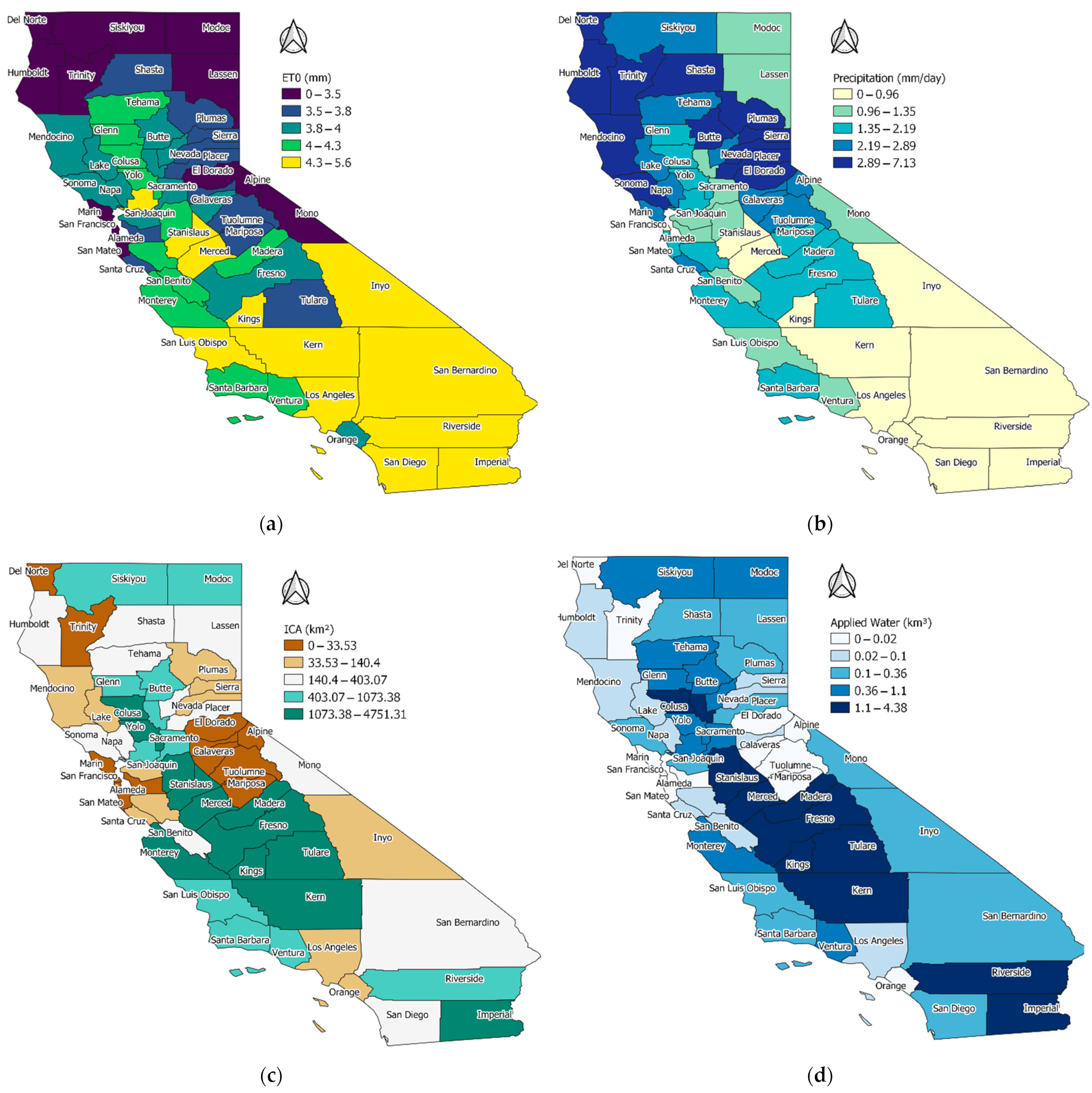
California’s Mediterranean climate—characterized by cold and wet winters and hot and dry summers—coupled with intricate infrastructure enabling widespread irrigation, makes the state ideal for cultivating a wide variety of crops [38]. California is the leading agricultural state in the United States in terms of farm-level sales. In 2020, California’s farms and ranches received $49.1 billion in cash receipts for their output, whereas almonds, grapes, pistachios, lettuce, and strawberries had the top valued commodities for the 2020 crop year [39]. Five of California’s counties—Fresno, Tulare, Monterey, Kern, and Merced—rank among the leading agricultural counties in the United States [40], whereas there is no farmland in San Francisco county. Different data sources and reports show that California irrigated agriculture accounts for roughly 40% to 80% of total water supplies. Therefore, it is very important for decision makers on a large scale to have accurate estimations of the required amount of irrigation water to manage water resources in a sustainable and efficient manner, especially in recent years, when the state has been under the stress of extreme heat due to climate change. It is also important to note that information about California’s agricultural production and water use is scarce and deals with uncertainty [41]. Therefore, any attempts to investigate the available data in more depth can cast light on their potential and, more importantly, determine the information gap. Figure 1 depicts annual reference evapotranspiration (ET₀), precipitation, irrigated crop area (ICA), and applied water at the county level, averaged over the 18-year time span of the current study.

1.2. Database and Data Management

Various input combinations have been studied to predict the total annual applied irrigation water, aligning with irrigation water demand at the county level across California.

Table 1. Input and output variables of the machine learning models.

Variable (Definition)	Acronym	Unit
Applied Water (the quantity of volumetric water applied to all crops in a county)	AW	km3 (Billion m3)
Irrigated Crop Area (the total amount of land irrigated for the purpose of growing a crop, including multi-cropping acres)	ICA	km2
Elevation (elevation above mean sea level)	El	m
Precipitation (daily accumulated precipitation)	Pr	mm
Daily maximum relative humidity	RHmax	%
Daily minimum relative humidity	RHmin	%
Daily mean downward shortwave radiation at the surface	Srad	W/m3
Daily mean wind speed	Wspd	m/s
Daily minimum temperature	Tmin	K
Daily maximum temperature	Tmax	K
Mean vapor pressure deficit	VPD	kPa
Reference evapotranspiration (short grass)	ET0	mm

shows the input and output variables of the machine learning models. It should be noted that the first row is the only output (i.e., target) of models and different models use various combinations of other variables as their input. All variables for each of the 58 counties of the California state are annual. The time span of the data is 18 years (1998–2015). Applied water and irrigated crop area data are acquired from the Department of Water Resources in the California Natural Resources Agency (CNRA) dataset, which is publicly available [36]. The source of all other meteorological and geological input data is Gridded Surface Meteorological (gridMET) Dataset, which is also publicly available [42]. The gridMET is a dataset of daily high spatial resolution surface meteorological data covering the contiguous US from 1979 to the present.

More than 400 different commodities are grown in California, with each crop having different agronomic practices and water demand. For simplification, the irrigated cropped areas were categorized into 20 crop categories and multi-crop areas, as shown in

Table 2. Categories of crops cultivated in California, according to [43].

Number	Crop Category	Acronym	Definition
1	Grain	GR	Wheat, barley, oats, miscellaneous grain and hay, and mixed grain and hay
2	Rice	RI	Rice and wild rice
3	Cotton	CO	Cotton
4	Sugar beet	SB	Sugar beets
5	Corn	CN	Corn (field and sweet)
6	Dry beans	DB	Beans (dry)
7	Safflower	SA	Safflower
8	Other field crops	FL	Flax, hops, grain sorghum, sudan, castor beans, miscellaneous fields, sunflowers, hybrid sorghum/sudan, millet, and sugar cane
9	Alfalfa	AL	Alfalfa and alfalfa mixtures
10	Pasture	PA	Clover, mixed pasture, native pastures, induced high water table native pasture, miscellaneous grasses, turf farms, bermuda grass, rye grass, and klein grass
11	Tomato (processing)	TP	Tomatoes for processing
12	Tomato (fresh)	TF	Tomatoes for market
13	Cucurbits	CU	Melons, squash, and cucumbers
14	Onion and garlic	OG	Onions and garlic
15	Potato	PO	Potatoes
16	Miscellaneous truck crops	TR	Artichokes, asparagus, beans (green), carrots, celery, lettuce, peas, spinach, flowers nursery and tree farms, bush berries, strawberries, peppers, broccoli, cabbage, cauliflower, and brussels sprouts
17	Almond and pistachios	AP	Almonds and pistachios
18	Other deciduous orchards	OR	Apples, apricots, cherries, peaches, nectarines, pears, plums, prunes, figs, walnuts, and miscellaneous deciduous
19	Citrus and subtropical	CS	Grapefruit, lemons, oranges, dates, avocados, olives, kiwis, jojoba, eucalyptus, and miscellaneous subtropical fruit
20	Vineyards	VI	Table grapes, wine grapes, and raisin grapes
21	Multi-cropping	MC	Multi-cropping

[43]. Multi-crop area is the acreage that is farmed more than once a year, often with different crops.

2. Methodology

After testing different machine learning models in the current study, the best one is chosen to predict county-level annual irrigation water use across California using several predictors’ combinations. All models are trained with county-level geographical and meteorological time series, along with irrigated cropped areas of each county as defined by the Department of Water Resources in the California Natural Resources Agency [36]. Twenty-one categories are considered to represent the state’s total agricultural production. All the raw data are collected from publicly available sources and are preprocessed prior to being used in the machine learning model. In addition to the synchronous data-driven models, lagged time series of irrigation water use were included to analyze the influence of irrigation water use of previous years on the water use of the year of interest.

2.1. Model Selection and Training

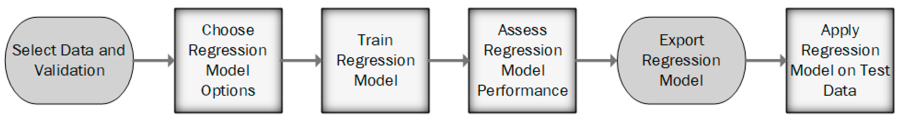
Using MATLAB (R2020a), several regression models have been trained to choose the best supervised machine learning model for predicting applied irrigation water, consisting of linear regression models, regression trees, Gaussian process regression models (GPR), Support Vector Machines (SVM), and ensembles of regression trees. Figure 2 shows a standard workflow for training regression models used in this study.

Two different approaches, consisting of stratified random sampling and simple random sampling, have been used for selecting test set. Stratified random sampling is a sampling method that involves taking samples of a population subdivided into smaller groups, called strata, so it takes random samples from stratified groups in proportion to the population. Conversely, a simple random sample is a sample of individuals in a population whereby the individuals are randomly selected from the whole population. The proportion of test sets was 10, 20, and 30 percent of the total data (1044 total datapoints). Statistical results were obtained from 10 different independent runs for each setting, whereas the proportion of train and test sets were the same in all runs. Linear regression models include simple linear, interactions linear, robust linear, and stepwise linear models. Regression trees modeled using three minimum leaf sizes had a fine tree (minimum leaf size is 4), medium tree (minimum leaf size is 12), and coarse tree (minimum leaf size is 36). Regression SVMs include linear SVMs and nonlinear SVMs (Quadratic, Cubic, and Gaussian). GPR models with different kernel functions include Rational Quadratic, Squared Exponential, Matern 5/2, and Exponential.

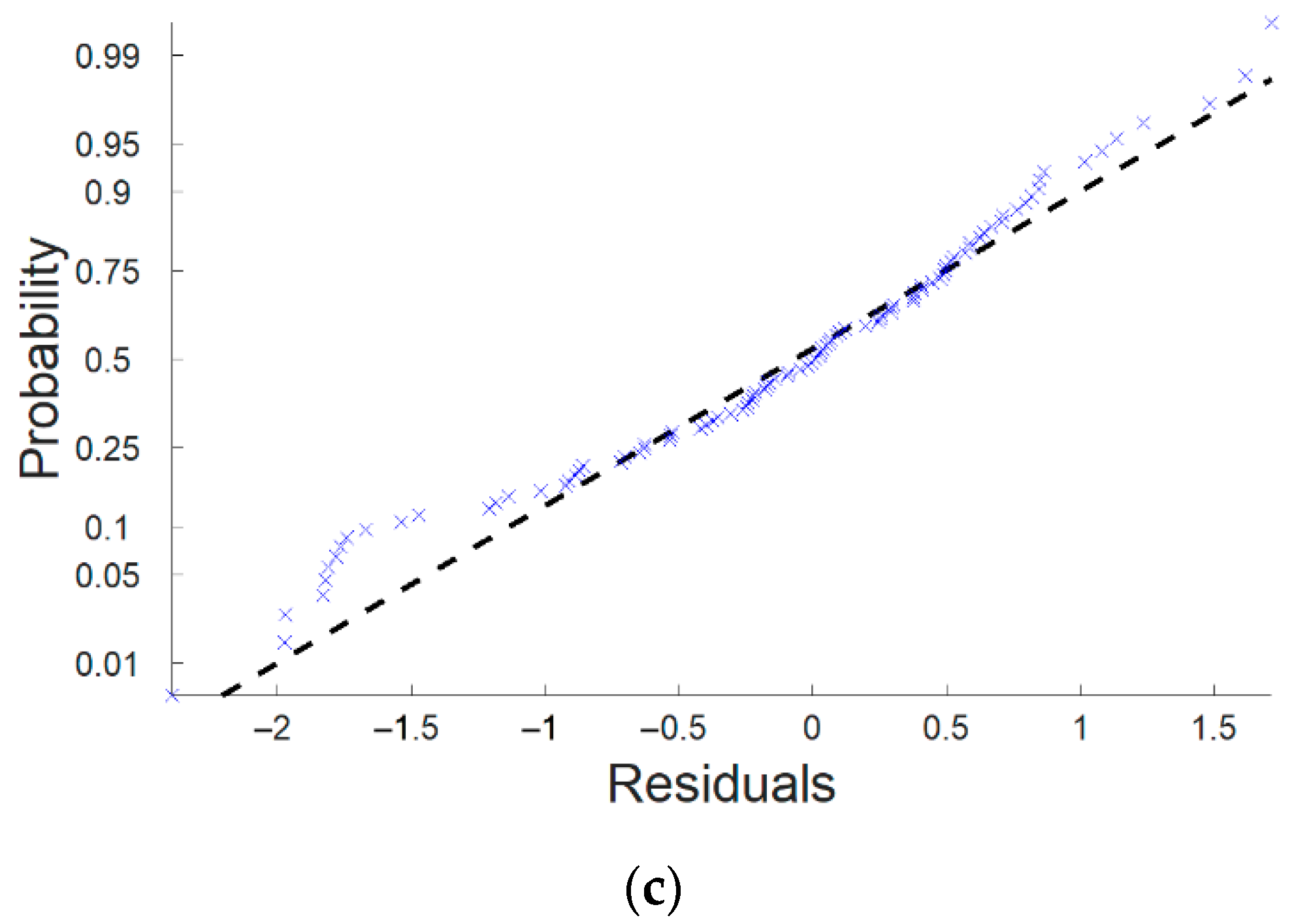
Trained regression models have been evaluated based on statistics, such as model error and residual (Figure 3). At this stage, all input categories and the whole timespan of the data were used in the model. Training and validation datasets were the same for all models to have a fair comparison between different models. To avoid overfitting, we employed the k-fold cross-validation method (k = 5). Therefore, the model statistics are computed using the observations in the k validation folds and the average values are reported. The GPR model has the best overall score among all regression models. We applied the Root Mean Square Error (RMSE) on the validation set as the model score. GPR as a nonparametric, kernel-based probabilistic model, uses the Bayesian approach to regression. Given the training set $\left\{\left(x_i,y_i\right);i=1,2,\dots ,n\right\}$, where $x_i\in {ℝ}^d$ and $y_i\in ℝ$, drawn from a distribution. A linear regression model is of the form $y=x^T\beta +\epsilon$, where $\epsilon$ has the distribution $N\left(0,{\sigma }^2\right)$ whereas the error variance ${\sigma }^2$ and the coefficients $\beta$ are estimated from the data. A GPR model explains the response by introducing latent variables, $f\left(x_i\right)$, $i=1,2,\dots ,n$, from a Gaussian process (GP), and explicit basis functions, $h$. A GP is a collection of random variables such that any subset of these variables is jointly Gaussian [44]. If $\left\{f\left(x\right), x\in {ℝ}^d\right\}$ is a GP, then given $n$ observations, the joint distribution of the random variables $f\left(x_1\right),f\left(x_2\right),\dots ,f\left(x_n\right)$ is Gaussian. Given a Gaussian process, which is specified by a mean ($m\left(x\right)$) and covariance function ($k\left(x,x^{\prime }\right)$), we can sample a function at the point $x$ from the Gaussian process according to $f\left(x\right)~GP(m\left(x\right),k\left(x,x^{\prime }\right)$. The covariance function $k\left(x,x^{\prime }\right)$ can be defined by various kernel functions. It can be parameterized in terms of the kernel parameters in vector θ. Hence, it is possible to express the covariance function as $k\left(x,x^{\prime }|\theta \right)$. The kernel parameters are based on the signal standard deviation ${\sigma }_f$ and the characteristic length scale ${\sigma }_l$; both need to be greater than 0, such that ${\theta }_1=\log {\sigma }_l$ and ${\theta }_2=\log {\sigma }_f$. In an isotropic kernel, the correlation length scales are the same for all the predictors, whereas, with a nonisotropic kernel, each predictor variable has its separate length scale. An instance of response $y$ in a GPR can be modeled as:

$$h{\left(x\right)}^T\beta +f\left(x\right) st f\left(x\right){\displaystyle ~}GP\left(0,k\left(x,x^{\prime }\right)\right)$$

(1)

$$P\left(y_i|f\left(x_i\right),x_i\right) {\displaystyle ~} N(y_i|h{\left(x_i\right)}^T\beta +f\left(x_i\right) , {\sigma }^2)$$

(2)

$$k\left(x,x^{\prime }\right)={\sigma }_f^2\left(1+\frac{\sqrt{5} r}{{\sigma }_l}+\frac{5r^2}{3{\sigma }_l^2}\right)\exp \left(-\frac{\sqrt{5} r}{{\sigma }_l}\right), r=\sqrt{{\left(x-x^{\prime }\right)}^T\left(x-x^{\prime }\right)}$$

(3)

where $f\left(x\right)$ is from a zero-mean GP with Matern 5/2 covariance function, $k\left(x,x^{\prime }\right)$. $h\left(x\right)$ is a set of basis functions that transform the original feature vector $x$ in ${ℝ}^d$ into a new feature vector $h\left(x\right)$ in ${ℝ}^p$. $\beta$ is a $p$-by−1 vector of basis function coefficients, and $r$ is the Euclidean distance between $x$ and $x^{\prime }$.

After choosing the GPR model to train, we used a Bayesian optimization scheme to select hyperparameter values. Different combinations of hyperparameter values have been tried in this procedure to minimize the model Mean Squared Error (MSE) and return a model with the optimized parameters.

Table 3. List of hyperparameters for Gaussian process regression model.

Parameter	Search Range	Optimal Value
Basis function coefficients	Zero, Constant, and Linear	Zero
Kernel function	Rational Quadratic, Squared Exponential, Matern 5/2, Matern 3/2, and Exponential	Matern 5/2
Kernel mode	Isotropic Kernel, Nonisotropic Kernel	Nonisotropic Kernel
Kernel scale	2.4338–2433.828	1747.9647
Sigma	Observation noise standard deviation	5.6562

contains the hyperparameters’ search range and optimized value.

Figure 3b,c show that the residuals are pretty symmetrically distributed, tending to cluster towards the middle of the plot, and the normal probability plot also shows no deviation from normality nor skewness on the distribution of residuals, indicating a decent fit for the data.

2.2. Input Data Combination

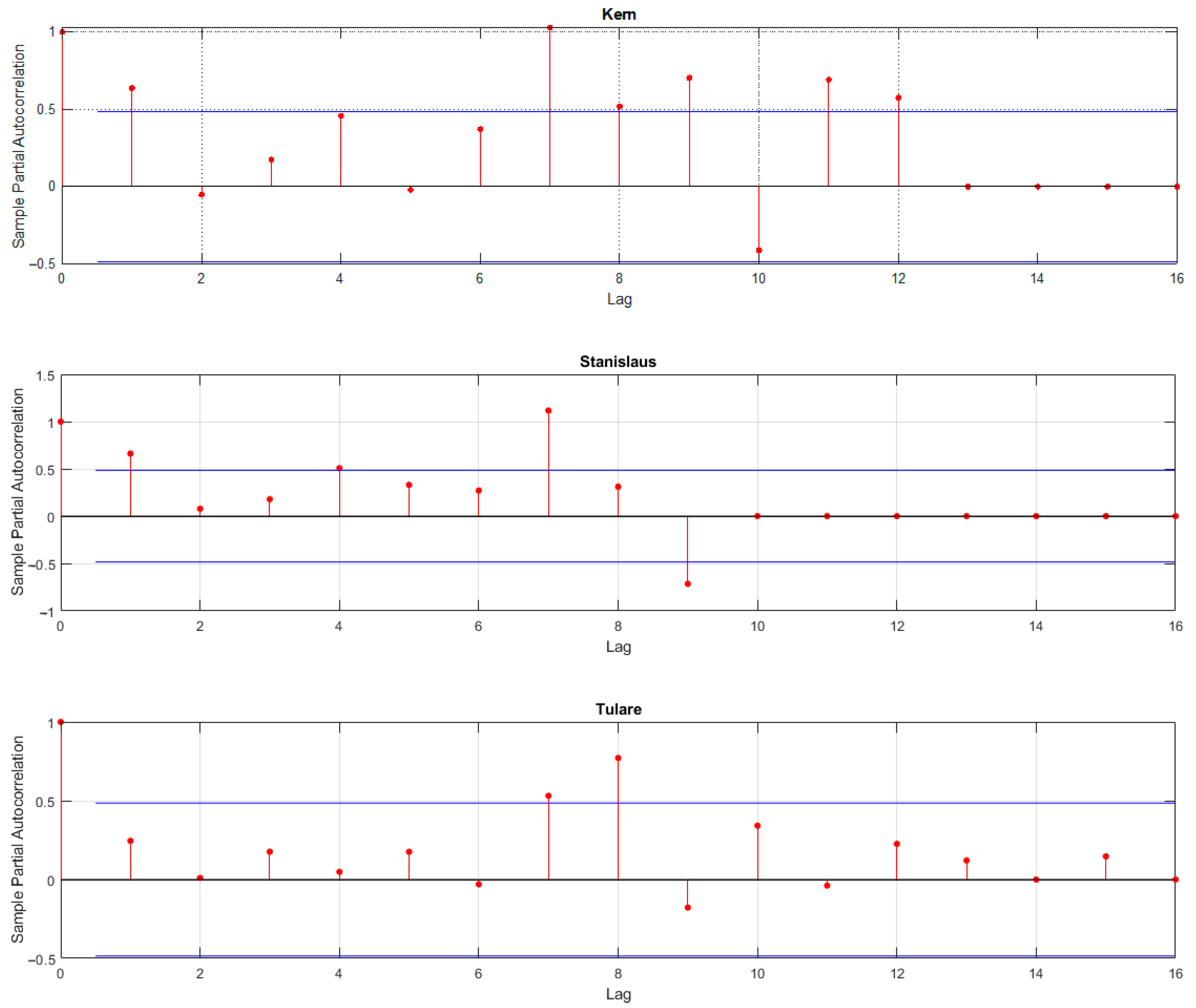
This study investigates several input variables with five combinations using the GPR method to predict irrigation water use. All input variables and combinations are listed in

Table 4. Input data combinations for the GPR model with total annual AW in a county as the response variable.

Model Name	Predictors
M1	ICAi:i = 1:21 *, ETcj, j = 1:20 ** Elevation, Precipitation, Maximum relative humidity, Minimum relative humidity, Surface radiation, Wind speed, Maximum air temperature, Minimum air temperature, Vapor pressure deficit, ETo grass
M2	ICAi:i = 1:21, Elevation, Precipitation, Maximum relative humidity, Minimum relative humidity, Surface radiation, Wind speed, Maximum air temperature, Minimum air temperature, Vapor pressure deficit, ETo grass
M3	ICAi:i = 1:21, Elevation, Precipitation, Maximum relative humidity, Minimum relative humidity, Surface radiation, Wind speed, Maximum air temperature, Minimum air temperature, ETo grass
M4	ICAi:i = 1:21, Precipitation, Maximum relative humidity, Minimum relative humidity, Surface radiation, Wind speed, Maximum air temperature, Minimum air temperature, ETo grass
M5	ICAi:i = 1:21, Precipitation, Maximum relative humidity, Minimum relative humidity, Surface radiation, Wind speed, Maximum air temperature, Minimum air temperature
M6	ICAi:i = 1:21 *, ETcj, j = 1:20 ** Elevation, Precipitation, Maximum relative humidity, Minimum relative humidity, Surface radiation, Wind speed, Maximum air temperature, Minimum air temperature, Vapor pressure deficit, ETo grass, IWU(t−1)
M7	ICAi:i = 1:21, Elevation, Precipitation, Maximum relative humidity, Minimum relative humidity, Surface radiation, Wind speed, Maximum air temperature, Minimum air temperature, Vapor pressure deficit, ETo grass, IWU(t−1)
M8	ICAi:i = 1:21, Elevation, Precipitation, Maximum relative humidity, Minimum relative humidity, Surface radiation, Wind speed, Maximum air temperature, Minimum air temperature, ETo grass, IWU(t−1)
M9	ICAi:i = 1:21, Precipitation, Maximum relative humidity, Minimum relative humidity, Surface radiation, Wind speed, Maximum air temperature, Minimum air temperature, ETo grass, IWU(t−1)
M10	ICAi:i = 1:21, Precipitation, Maximum relative humidity, Minimum relative humidity, Surface radiation, Wind speed, Maximum air temperature, Minimum air temperature, IWU(t−1)

* i is an index for crop categories in Table 2. ** j is an index for crop categories in Table 2, excluding multi-crop areas.

. The effect of water use in previous years was studied in the second step. The number of lags for the response variable is selected according to the partial autocorrelation function (PACF) of annual irrigation water use in each county. Partial autocorrelation explains the relationship between an observation in a time series with observations at previous time steps, whereas the indirect correlations are removed. PACF analyses show that in 43.8% of counties, 1-year lag significantly affects IWU. Figure 4 shows the PACF analyses for some counties with the highest ICA. The pattern shows significant correlations at the first or second lag, followed by correlations that are not significant. This pattern indicates an autoregressive term in the data, and the number of significant correlations indicates the order of the autoregressive term. As mentioned in Table 4, M6-M10 includes one year lag for irrigation water use (IWU_t−1) based on the PACF analysis.

The performance of the models is evaluated using the following four error-based criteria along with the coefficient of determination (R²): Root Mean Square Error (RMSE), Mean Absolute Error (MAE), Root Mean Square Percentage Error (RMSPE), and Normalized Mean Squared Error by the mean of actual data (NRMSE_m).

$$RMSE={\left[\frac{1}{n}{\displaystyle \sum }_{i=1}^n{\left(A{W}_{Act}-A{W}_{Est}\right)}^2\right]}^{\raisebox{1ex}{$1$}\!\left/ \!\raisebox{-1ex}{$2$}\right.}$$

(4)

$$MAE=\frac{1}{n}{\displaystyle \sum }_{i=1}^n\left|A{W}_{Act}-A{W}_{Est}\right|$$

(5)

$$RMSPE={\left[\frac{100}{n}{\displaystyle \sum }_{i=1}^n{\left(\frac{\left|A{W}_{Act}-A{W}_{Est}\right|}{\left|A{W}_{Act}\right|}\right)}^2\right]}^{\raisebox{1ex}{$1$}\!\left/ \!\raisebox{-1ex}{$2$}\right.}$$

(6)

$$NRMSE\_m=\frac{RMSE}{{\overline{AW}}_{Act}}$$

(7)

where $A{W}_{Act}$ is desired output or actual applied water, $A{W}_{Est}$ is the model output or estimated applied water, and $n$ is size of the dataset.

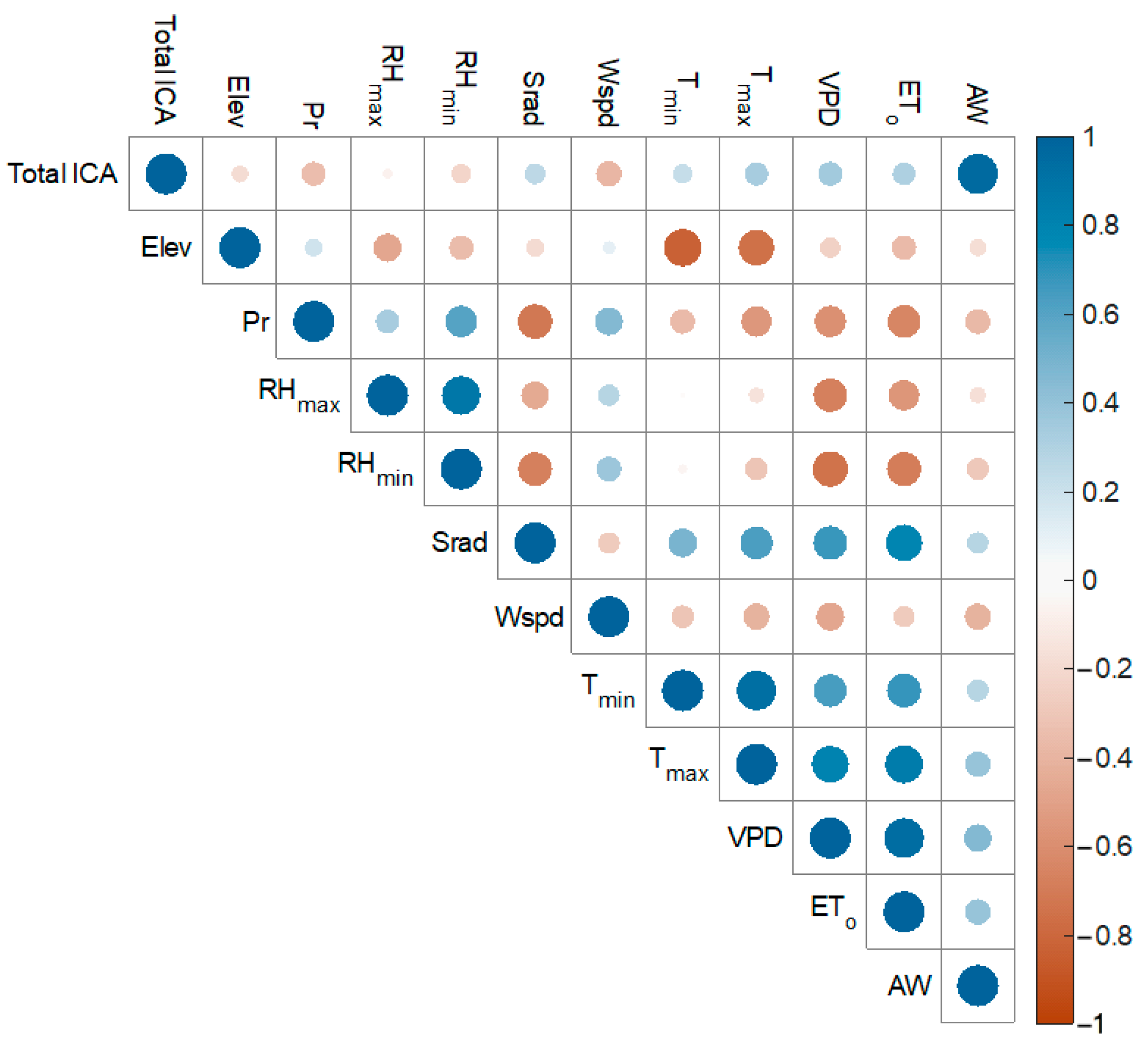
Figure 5 shows the linear correlation between variables introduced in Table 1. As the Pearson correlation coefficient is a normalized measure of the covariance (i.e., the covariance of two variables divided by their standard deviations), its value always falls between 1 and −1. The higher the absolute value of the correlation coefficient, the higher the association and relationship between the two variables. In other words, when R (the correlation coefficient) between two variables is zero, there is no linear relationship between them, and when the absolute value of R approaches 1, the linear relationship between the variables becomes stronger.

3. Results and Discussion

Figure 5 indicates that the applied water positively correlates with the irrigated crop area. This implies that the volume of irrigation water demand can be estimated by having reliable and accurate data on cropped areas. This is especially important because the data on irrigation water use is very hard to achieve and, at the same time, of great importance for water management and decision makers. On the other hand, the cropped area can be estimated easily using remote sensing data. For example, Landsat satellite data are publicly available with a temporal resolution of 8 or 16 days and a spatial resolution of 30 m. This data can be used as an estimator of irrigation water use globally. Although, it should be noted that the exact amount of irrigation water demand relies on meteorological factors, crop type and variety, and field management.

Figure 5 also shows higher precipitation and humidity associated with lower applied water. It is logical to infer that less irrigation is required in regions with higher precipitation and humidity. Figure 5 also shows that temperature and evapotranspiration positively correlate with applied water. The negative correlation between wind speed and irrigation water demand seems counterintuitive because higher wind speeds are associated with a higher evaporating force of the atmosphere and, therefore, higher water loss. Although, it should be noted that wind speed also has a negative correlation with temperature and a positive correlation with humidity.

Table 5. ANOVA test results.

	df	SS	MS	F	Significance F
Regression	11	912.4558127	82.95052842	1508.74493	0
Residual	1001	55.03480246	0.054979823
Total	1012	967.4906151

and

Table 6. Parameter estimates for models’ variables.

	Estimate	Standard Error	t Stat	p-Value	Lower 95%	Upper 95%
Intercept	19.1920	4.8588	3.9499	0.0001	9.6574	28.7267
ICA	0.0009	0.0000	99.2910	0.0000	0.0009	0.0009
El	−0.0001	0.0001	−2.0762	0.0381	−0.0003	0.0000
Pr	−0.0270	0.0092	−2.9374	0.0034	−0.0450	−0.0090
RHmax	−0.0008	0.0033	−0.2475	0.8046	−0.0074	0.0057
RHmin	0.0091	0.0060	1.5237	0.1279	−0.0026	0.0209
Srad	−0.0032	0.0019	−1.6533	0.0986	−0.0069	0.0006
Wspd	0.0231	0.0286	0.8073	0.4197	−0.0330	0.0791
Tmin	0.0335	0.0122	2.7502	0.0061	0.0096	0.0574
Tmax	−0.0984	0.0206	−4.7681	0.0000	−0.1389	−0.0579
VPD	1.1808	0.1394	8.4703	0.0000	0.9072	1.4543
ET0	−0.1056	0.0968	−1.0908	0.2756	−0.2955	0.0843

demonstrate the results of the analysis of variance (ANOVA) test of the multiple linear regression model predicting irrigation applied water as the target. According to Table 1, 11 inputs are considered for this multiple linear regression. The high value of the sum of squares (SS) and mean squares (MS) of the model against the residual and the high value of the F-test statistic reject the null hypothesis that the factor of all variables is equal to zero. In other words, the results of the ANOVA test suggest the capability of input variables in explaining the variations in the target variable and, therefore, their effectiveness in predicting the irrigation applied water.

The Table 6 is the parameter estimates that summarize the effect of each predictor. In this analysis, the lower the p-value of a predictor, the higher its effect and significance in predicting the target value. Therefore, irrigated crop area, maximum temperature, and vapor pressure deficit are the most influential parameters in predicting the irrigation applied water in California. Precipitation and minimum temperature are other important variables, whereas relative humidity and wind speed are the least significant parameters in irrigation water demand prediction. It should be noted that although relative humidity and wind speed are some of the deriving forces of the atmosphere’s evaporating demand, according to Table 5 and Table 6, their significance falls behind other deriving forces, such as air temperature and solar radiation, which control sensible heat and net radiation, respectively. This is not surprising because different atmospheric deriving forces have various levels of significance in each climate. In addition, as relative humidity is a mixed factor based on air temperature and humidity, and both air temperature and humidity effects are considered in the model through Tmax and VPD, respectively, the model might have found relative humidity redundant and, therefore, not significant. The same reasoning can be used to explain the low importance of ETo; because all the important deriving forces are already present in the input data, the model finds the effect of ETo insignificant.

As

Table 7. Performance indices for all models.

Model	M1	M2	M3	M4	M5	M6	M7	M8	M9	M10
R2	0.9945	0.9828	0.9825	0.9792	0.9814	0.9949	0.9760	0.9760	0.9768	0.9776
RMSE (km3)	0.0669	0.1185	0.1197	0.1303	0.1232	0.0642	0.1401	0.1399	0.1376	0.1351
MAE (km3)	0.0335	0.0550	0.0556	0.0617	0.0556	0.0322	0.0616	0.0632	0.0624	0.0603
STD_predict	0.9084	0.9203	0.9138	0.9188	0.9134	0.9089	0.9281	0.9287	0.9266	0.9270
RMSPE	4.2218	7.6086	5.5558	2.4232	4.0605	3.9646	2.7092	2.4763	2.6975	2.3970
NRMSE	0.1071	0.1897	0.1916	0.2085	0.1972	0.1028	0.2242	0.2240	0.2202	0.2162

illustrates, all ten variable combinations are capable of predicting the irrigation water applied accurately. Based on root mean square error (RMSE) values, models M6 and M1 are the best models. Both of these models have the most influential variables based on parameter estimates (i.e., air temperature, VPD, and ICA) in their inputs. The main difference between these two models is that Model 6 considers the IWA in previous time steps as well, whereas model 1 only uses the inputs at the same time as the model’s target. Considering the similar performance of these two models, it can be inferred that even without knowledge of the amount of applied water in previous time steps, the presented ML model is capable of predicting the irrigation demand. This is of especially great importance in ungauged areas without a reliable record of irrigation data.

Although Table 7 indicates the strength of our approach in predicting irrigation water demand in California, it should be noted that just like any data-driven approach, the accuracy and reliability of this model depend on the input data. The findings of this research show that machine learning can predict the irrigation water demand with high accuracy. Still, the main limitation is that the input data of this model is based on observations and measurements, whereas the outputs are from other models that deal with different levels of uncertainty. This might be the main limitation and drawback of this research and any other similar attempt to use data-driven models for predicting water demand on a large scale. To tackle this shortcoming, managing organizations and policy makers should pay more attention to generating more reliable large-scale data based on observations and measurements. However, it should be noted that although it is clear what variables are influencing the irrigation water demand (as mentioned earlier in this study and showed statistically through our findings), their real-world physical interactions are too complicated to be simulated. On the other hand, data-driven approaches are capable of modeling this complexity without requiring the exact knowledge of the hidden multi-dimensional interactions.

4. Conclusions

In many parts of the world, agriculture is the largest water-consuming sector, and therefore, estimating the volumetric water demand is of great importance for stakeholders involved in regulating freshwater consumption for sustainable use. Traditional methods involve using a combination of water balance, crop models, and satellite-based remote sensing for better estimation accuracy and for higher spatial resolution.

The challenge with this approach is the dependency on a large dataset, often unavailable or broadly estimated, and on complex models that require experts and time to manipulate and integrate different climatic, agronomic, and environmental scenarios. In this regard, data-driven models present a promising technique whereby a combination of modeled, measured, and reported through agricultural census datasets can be used to generate useful outputs without the need for the mathematical representation of the entire biophysical process. Such an approach can also limit the number of input parameters with limited or no compromise on the accuracy of the output, that in this case is the volumetric agricultural water demand. Using California State as the study site, the findings of this study show the strength of the correlation between meteorological, geographical, and cropped areas with the applied irrigation water. California was chosen as the study site for its crop diversity, spatial and temporal climatic variability, and for the need to control and regulate agricultural water usage. We found that irrigated cropped area, air temperature, and vapor pressure deficit are the most significant variables in predicting irrigation water demand. In addition, among various regression machine learning approaches, Gaussian process regression (GPR) produced the best results in predicting irrigation water demand (R² higher than 0.97 and RMSE as low as 0.06 km³) with different input variable combinations.

We hypothesize that this approach could be scaled up or down depending on data availability, but it can also be extrapolated to other regions where biophysical models are too complex to use and/or where input data are limited.

The proposed machine learning approach will be converted to a simple web-based tool whereby stakeholders can interactively create and evaluate cropping patterns and climatic change scenarios on consumptive agricultural use. Although this can be achieved using the traditional biophysical/hydrological models, the implementation of those scenarios can be time consuming and computationally prohibitive for stakeholders and policy makers often interested in the big picture. The temporal and spatial resolution of the prediction can be improved, especially with the help of remote sensing data. However, the availability of consumptive water use and the accuracy of that reported remain the main challenge for this approach. Until then, the data-driven approach will continue to rely on physical and remote sensing models for training. Therefore, a data-driven approach, in general, cannot and should not substitute the traditional biophysical modeling. However, combining the two approaches will bring a lot of computational benefits and overcome the limitation of data availability and gaps.

References

- Bayer, P.E.; Edwards, D. Machine learning in agriculture: From silos to marketplaces. Plant Biotechnol. J. 2020, 19, 648–650. [Google Scholar] [CrossRef] [PubMed]
- Liakos, K.G.; Busato, P.; Moshou, D.; Pearson, S.; Bochtis, D. Machine learning in agriculture: A review. Sensors 2018, 18, 2674. [Google Scholar] [CrossRef] [PubMed] [Green Version]
- Tantalaki, N.; Souravlas, S.; Roumeliotis, M. Data-driven decision making in precision agriculture: The rise of big data in agricultural systems. J. Agric. Food Inf. 2019, 20, 344–380. [Google Scholar] [CrossRef]
- Vasisht, D.; Kapetanovic, Z.; Won, J.; Jin, X.; Chandra, R.; Sinha, S.; Kapoor, A.; Sudarshan, M.; Stratman, S. Farmbeats: An IoT platform for data-driven agriculture. In Proceedings of the 14th {USENIX} Symposium on Networked Systems Design and Implementation ({NSDI} 17), Boston, MA, USA, 27–29 March 2017; pp. 515–529. [Google Scholar]
- Chlingaryan, A.; Sukkarieh, S.; Whelan, B. Machine learning approaches for crop yield prediction and nitrogen status estimation in precision agriculture: A review. Comput. Electron. Agric. 2018, 151, 61–69. [Google Scholar] [CrossRef]
- Crane-Droesch, A. Machine learning methods for crop yield prediction and climate change impact assessment in agriculture. Environ. Res. Lett. 2018, 13, 114003. [Google Scholar] [CrossRef] [Green Version]
- Van Klompenburg, T.; Kassahun, A.; Catal, C. Crop yield prediction using machine learning: A systematic literature review. Comput. Electron. Agric. 2020, 177, 105709. [Google Scholar] [CrossRef]
- Ahmadi, A.; Emami, M.; Daccache, A.; He, L. Soil Properties Prediction for Precision Agriculture Using Visible and Near-Infrared Spectroscopy: A Systematic Review and Meta-Analysis. Agronomy 2021, 11, 433. [Google Scholar] [CrossRef]
- Ebrahimi, M.A.; Khoshtaghaza, M.H.; Minaei, S.; Jamshidi, B. Vision-based pest detection based on SVM classification method. Comput. Electron. Agric. 2017, 137, 52–58. [Google Scholar] [CrossRef]
- Pantazi, X.E.; Tamouridou, A.A.; Alexandridis, T.K.; Lagopodi, A.L.; Kontouris, G.; Moshou, D. Detection of Silybum marianum infection with Microbotryum silybum using VNIR field spectroscopy. Comput. Electron. Agric. 2017, 137, 130–137. [Google Scholar] [CrossRef]
- Pantazi, X.E.; Moshou, D.; Bravo, C. Active learning system for weed species recognition based on hyperspectral sensing. Biosyst. Eng. 2016, 146, 193–202. [Google Scholar] [CrossRef]
- Emami, M.; Nazif, S.; Mousavi, S.F.; Karami, H.; Daccache, A. A hybrid constrained coral reefs optimization algorithm with machine learning for optimizing multi-reservoir systems operation. J. Environ. Manag. 2021, 286, 112250. [Google Scholar] [CrossRef]
- El Bilali, A.; Taleb, A. Prediction of irrigation water quality parameters using machine learning models in a semi-arid environment. J. Saudi Soc. Agric. Sci. 2020, 19, 439–451. [Google Scholar] [CrossRef]
- Navarro-Hellín, H.; Martinez-del-Rincon, J.; Domingo-Miguel, R.; Soto-Valles, F.; Torres-Sánchez, R. A decision support system for managing irrigation in agriculture. Comput. Electron. Agric. 2016, 124, 121–131. [Google Scholar] [CrossRef] [Green Version]
- Torres-Sanchez, R.; Navarro-Hellin, H.; Guillamon-Frutos, A.; San-Segundo, R.; Ruiz-Abellón, M.C.; Domingo-Miguel, R. A decision support system for irrigation management: Analysis and implementation of different learning techniques. Water 2020, 12, 548. [Google Scholar] [CrossRef] [Green Version]
- Goap, A.; Sharma, D.; Shukla, A.K.; Krishna, C.R. An IoT based smart irrigation management system using machine learning and open source technologies. Comput. Electron. Agric. 2018, 155, 41–49. [Google Scholar] [CrossRef]
- Vij, A.; Vijendra, S.; Jain, A.; Bajaj, S.; Bassi, A.; Sharma, A. IoT and machine learning approaches for automation of farm irrigation system. Procedia Comput. Sci. 2020, 167, 1250–1257. [Google Scholar] [CrossRef]
- Goldstein, A.; Fink, L.; Meitin, A.; Bohadana, S.; Lutenberg, O.; Ravid, G. Applying machine learning on sensor data for irrigation recommendations: Revealing the agronomist’s tacit knowledge. Precis. Agric. 2018, 19, 421–444. [Google Scholar] [CrossRef]
- Mekonnen, Y.; Namuduri, S.; Burton, L.; Sarwat, A.; Bhansali, S. Machine learning techniques in wireless sensor network based precision agriculture. J. Electrochem. Soc. 2019, 167, 037522. [Google Scholar] [CrossRef]
- Pulido-Calvo, I.; Montesinos, P.; Roldán, J.; Ruiz-Navarro, F. Linear regressions and neural approaches to water demand forecasting in irrigation districts with telemetry systems. Biosyst. Eng. 2007, 97, 283–293. [Google Scholar] [CrossRef]
- Zhang, J.; Li, H.; Shi, X.; Hong, Y. Wavelet-nonlinear cointegration prediction of irrigation water in the irrigation district. Water Resour. Manag. 2019, 33, 2941–2954. [Google Scholar] [CrossRef]
- Khan, M.A.; Islam, M.Z.; Hafeez, M. Evaluating the Performance of Several Data Mining Methods for Predicting Irrigation Water Requirement. In Proceedings of the Tenth Australasian Data Mining Conference, Sidney, Australia, 5–7 December 2012; Australian Computer Society, Inc.: Sydney, Australia, 2012; pp. 199–207. [Google Scholar]
- Qin, Y.; Mueller, N.D.; Siebert, S.; Jackson, R.B.; AghaKouchak, A.; Zimmerman, J.B.; Tong, D.; Hong, C.; Davis, S.J. Flexibility and intensity of global water use. Nat. Sustain. 2019, 2, 515–523. [Google Scholar] [CrossRef]
- Atsalakis, G.; Minoudaki, C.; Markatos, N.; Stamou, A.; Beltrao, J.; Panagopoulos, T. Daily irrigation water demand prediction using adaptive neuro-fuzzy inferences systems (ANFIS). In Proceedings of the 3rd IASME/WSEAS International Conference on Energy, Environment, Ecosystems & Sustainable Development (EEESD’07), Agios Nikolaos, Greece, 24–26 July 2007; World Scientific and Engineering Academy and Society Press (WSEAS Press): Agios Nikolaos, Greece, 2007. [Google Scholar]
- Mo, X.; Liu, S.; Lin, Z.; Xu, Y.; Xiang, Y.; McVicar, T.R. Prediction of crop yield, water consumption and water use efficiency with a SVAT-crop growth model using remotely sensed data on the North China Plain. Ecol. Model. 2005, 183, 301–322. [Google Scholar] [CrossRef]
- Weatherhead, E.K.; Knox, J.W. Predicting and mapping the future demand for irrigation water in England and Wales. Agric. Water Manag. 2000, 43, 203–218. [Google Scholar] [CrossRef]
- Wada, Y.; Wisser, D.; Eisner, S.; Flörke, M.; Gerten, D.; Haddeland, I.; Hanasaki, N.; Masaki, Y.; Portmann, F.T.; Stacke, T.; et al. Multimodel projections and uncertainties of irrigation water demand under climate change. Geophys. Res. Lett. 2013, 40, 4626–4632. [Google Scholar] [CrossRef] [Green Version]
- Wisser, D.; Frolking, S.; Douglas, E.M.; Fekete, B.M.; Vörösmarty, C.J.; Schumann, A.H. Global irrigation water demand: Variability and uncertainties arising from agricultural and climate data sets. Geophys. Res. Lett. 2008, 35, L24408. [Google Scholar] [CrossRef] [Green Version]
- Ehteram, M.; Allawi, M.F.; Karami, H.; Mousavi, S.-F.; Emami, M.; El-Shafie, A.; Farzin, S. Optimization of Chain-Reservoirs’ Operation with a New Approach in Artificial Intelligence. Water Resour Manag. 2017, 31, 2085–2104. [Google Scholar] [CrossRef]
- Ehteram, M.; Mousavi, S.-F.; Karami, H.; Farzin, S.; Emami, M.; Othman, F.B.; Amini, Z.; Kisi, O.; El-Shafie, A. Fast convergence optimization model for single and multi-purposes reservoirs using hybrid algorithm. Adv. Eng. Inform. 2017, 32, 287–298. [Google Scholar] [CrossRef]
- Mehta, V.K.; Haden, V.R.; Joyce, B.A.; Purkey, D.R.; Jackson, L.E. Irrigation demand and supply, given projections of climate and land-use change, in Yolo County, California. Agric. Water Manag. 2013, 117, 70–82. [Google Scholar] [CrossRef]
- Ahmadi, A.; Nasseri, M.; Solomatine, D.P. Parametric uncertainty assessment of hydrological models: Coupling UNEEC-P and a fuzzy general regression neural network. Hydrol. Sci. J. 2019, 64, 1080–1094. [Google Scholar] [CrossRef]
- Ahmadi, A.; Nasseri, M. Do direct and inverse uncertainty assessment methods present the same results? J. Hydroinformatics 2020, 22, 842–855. [Google Scholar] [CrossRef]
- Ahmadi, A.; Kerachian, R.; Skardi, M.J.E.; Abdolhay, A. A stakeholder-based decision support system to manage water resources. J. Hydrol. 2020, 589, 125138. [Google Scholar] [CrossRef]
- Loucks, D.P.; Da Costa, J.R. (Eds.) Decision Support Systems: Water Resources Planning; Springer Science & Business Media: Berlin/Heidelberg, Germany, 2013; Volume 26. [Google Scholar]
- California Department of Water Resources. Agricultural Land & Water Use Estimates, 2019–2020; California Department of Water Resources: Sacramento, CA, USA, 2020. Available online: https://water.ca.gov/Programs/Water-Use-And-Efficiency/Land-And-Water-Use/Agricultural-Land-And-Water-Use-Estimates (accessed on 1 February 2021).
- Wilson, T.S.; Sleeter, B.M.; Cameron, D.R. Future land-use related water demand in California. Environ. Res. Lett. 2016, 11, 054018. [Google Scholar] [CrossRef]
- Parker, L.E.; McElrone, A.J.; Ostoja, S.M.; Forrestel, E.J. Extreme heat effects on perennial crops and strategies for sustaining future production. Plant Sci. 2020, 295, 110397. [Google Scholar] [CrossRef] [PubMed]
- California Department of Food and Agriculture. Agricultural Statistics Review, 2019–2020; California Department of Food and Agriculture: Sacramento, CA, USA, 2020.
- Johnson, R.; Cody, B.A. California Agricultural Production and Irrigated Water Use; Congressional Research Service: Sacramento, CA, USA, 2015; p. 28. [Google Scholar]
- Cooley, H. California Agricultural Water Use: Key Background Information; Pacific Institute: Oakland, CA, USA, 2015; pp. 1–9. [Google Scholar]
- Abatzoglou, J.T. Development of gridded surface meteorological data for ecological applications and modelling. Int. J. Climatol. 2013, 33, 121–131. Available online: https://www.climatologylab.org/gridmet.html (accessed on 1 February 2021). [CrossRef]
- Orang, M.N.; Snyder, R.L.; Shu, G.; Hart, Q.J.; Sarreshteh, S.; Falk, M.; Beaudette, D.; Hayes, S.; Eching, S. California simulation of evapotranspiration of applied water and agricultural energy use in California. J. Integr. Agric. 2013, 12, 1371–1388. [Google Scholar] [CrossRef]
- Rasmussen, C.; Williams, C. Gaussian Processes for Machine Learning; MIT Press: Cambridge, MA, USA, 2006. [Google Scholar]
Figure 1.
Geographic depiction of key information relating to the irrigation water demand of California counties; (a) mean daily reference evapotranspiration (mm), (b) annual average daily precipitation (mm/day), (c) mean annual irrigated crop area (km2), and (d) mean annual applied irrigation water (km3).
Figure 2.
Common workflow for evaluating regression models used in the current study.
Figure 3.
(a) Estimated applied water vs. actual AW, (b) residuals for the estimated AW, and (c) normal probability plot of residuals.
Figure 4.
PACF graph for Fresno, Kern, Stanislaus, and Tulare.
Figure 5.
Pearson correlation coefficients of the models’ variables.