
Reclaimed Water Reuse for Groundwater Recharge: A Review of Hot Spots and Hot Moments in the Hyporheic Zone


1
Beijing Key Laboratory of Water Resources & Environmental Engineering, China University of Geosciences (Beijing), Beijing 100083, China
2
School of Water Resources and Environment, China University of Geosciences (Beijing), Beijing 100083, China
*
Author to whom correspondence should be addressed.
Water 2022, 14(12), 1936; https://doi.org/10.3390/w14121936
Submission received: 14 May 2022
/
Revised: 13 June 2022
/
Accepted: 14 June 2022
/
Published: 16 June 2022
(This article belongs to the Special Issue Water Reclamation and Reuse in a Changing World)
Abstract
:As an alternative resource, reclaimed water is rich in the various nutrients and organic matter that may irreparably endanger groundwater quality through the recharging process. During groundwater recharge with reclaimed water, hot spots and hot moments (HSHMs) in the hyporheic zones, located at the groundwater–reclaimed water interface, play vital roles in cycling and processing energy, carbon, and nutrients, drawing increasing concern in the fields of biogeochemistry, environmental chemistry, and pollution treatment and prevention engineering. This paper aims to review these recent advances and the current state of knowledge of HSHMs in the hyporheic zone with regard to groundwater recharge using reclaimed water, including the generation mechanisms, temporal and spatial characteristics, influencing factors, and identification indicators and methods of HSHMs in the materials cycle. Finally, the development prospects of HSHMs are discussed. It is hoped that this review will lead to a clearer understanding of the processes controlling water flow and pollutant flux, and that further management and control of HSHMs can be achieved, resulting in the development of a more accurate and safer approach to groundwater recharge with reclaimed water.

1. Introduction
With the increase in population, lifestyle changes, and the expansion of industrial and agricultural activities, aquifer recharges, fluxes, and contaminant infiltration have been substantially impacted, and thus water scarcity has become a global problem [1,2,3,4,5]. The United Nations has estimated that 2.7 billion people will face water shortages by 2025 [6]. Accordingly, increasing attention is being paid to the sustainable utilization of water resources [7]. As a result, reclaimed water is being widely used as a potential alternative water source, with the highest annual reclaimed water consumption in China, Mexico, and the United States [8].
Several technologies are used to treat wastewater, including ozonation, ultrafiltration, membrane bioreactor systems, forward osmosis, reverse osmosis, advanced oxidation, chlorine disinfection, nanofiltration, and ozone disinfection [9,10,11,12,13]. Nevertheless, it is difficult to completely remove all contaminants from reclaimed water. Studies have shown that irrigation with reclaimed water is beneficial to crop growth because nutrients such as nitrogen and phosphorus in reclaimed water can increase soil fertility [14,15,16]. However, with the deepening of the research on reclaimed water, it has been found that reclaimed water after treatment still contains problematic micropollutants, such as perfluorinated compounds (PFCs) [17], endocrine-disrupting chemicals [18,19,20,21], pharmaceuticals and personal care products (PPCPs) [22,23], antibiotics [24,25], antibiotic resistance genes [26,27], antibiotic-resistant bacteria [28,29], and pathogens [30,31], which may pose risks to environmental quality and human health.
Groundwater recharge with reclaimed water mainly includes irrigation using wells, surface spreading, and riverbank filtration (RBF). Riverbank filtration has proven to be a low-cost and energy-efficient alternative to traditional and advanced drinking water treatments [32,33]. Ding et al. [34] suggested that surface spreading with reclaimed water had much less impact on groundwater quality than direct injection due to the purification effect of river sediments. Therefore, RBF has been widely used globally to improve the water quality of urban water plants [35]. The study in this paper focuses on the hot spots and hot moments (HSHMs) during groundwater recharge with reclaimed water through riverbank filtration.
The HSHMs of material transformation determine the destination of most substances and the influence of reclaimed water on groundwater quality. During groundwater recharge with reclaimed water, the interaction between reclaimed water and groundwater and the exchange process between them produce significant changes in the physical and chemical water quality characteristics, and these changes occur mainly in the hyporheic zone [36]. The hyporheic zone is a complex place and a time-dynamic area [37,38]. In the hyporheic zone, especially during the process of groundwater recharge using reclaimed water, steep physical, chemical, and biogeochemical gradients at the interface tend to result in an active biogeochemical process, and a local enhancement of biogeochemical activity may occur [39,40], called HSHMs, that may have a disproportionate impact on the cycling of energy, carbon, and nutrients [41]. Regarding this disproportionate contribution, we have addressed related research in multiple fields, including hydrochemical evolution [42,43,44], environmental pollution [45,46,47,48,49], human health risk assessment [50], pollution control [51,52,53], and the survival of fish or invertebrates [54,55].
As unique phenomena arising during reclaimed water artificial recharge processes, HSHMs occur when geological heterogeneity is high and reaction conditions are met. Reaction conditions include: (i) the presence of reactants (including electron donors and electron acceptors); (ii) adequate advective conditions; and (iii) a continuous supply of reactants [56]. RBF provides the most favorable conditions for the occurrence of HSHMs.
Spatially, the structure of the aquifer media, the spatial distribution of geochemical substances, and the microorganisms are highly heterogeneous. In addition, on the time scale, the recharge rate, water chemistry, and temperature are time-varying. This heterogeneous and time-varying nature causes HSHMs to be difficult to capture.
According to statistics, although hot spots only occupy less than 2% of the study area, they explain up to 99% of the reactions [57,58,59,60]. Figure 1 illustrates the relationship between sediment volume, time, and process rates. The reaction rates in most sediment volumes are very low. Hot spots occupy only small volumes, but the reaction rates are relatively high. Hot moments are periods of high-speed reaction. As shown in Figure 1, the raised red parts are HSHMs.
Although some studies have explored the influencing factors of HSHMs, there are few studies with detailed explanations. As for the environmental problems caused by HSHMs associated with aquifer recharge using reclaimed water, we urgently need to identify HSHMs and find methods and indicators that can signal HSHMs for the management and control of the pollution of reclaimed water recharge. However, a summary of methods and indicators for identifying HSHMs has not been provided in previous studies. In this review, we summarize the features of HSHMs in the process of groundwater recharge with reclaimed water, including the spatial and temporal characteristics, influence factors, identification indicators, and methods. We focus on the HSHMs in reclaimed water reuse for two reasons: (i) the HSHMs of material transformation determine the destination of most substances and the influence of reclaimed water on groundwater quality; and (ii) the influencing factors of HSHMs are explained in detail, and the identification indicators are summarized to provide guidelines for future studies on reclaimed water reuse.
The purpose of this paper is to provide a comprehensive and systematic summary of the formation mechanisms, influencing factors, and identification methods of HSHMs formed during groundwater recharge with reclaimed water. This study on HSHMs can provide a scientific basis for substance cycling in the process of reclaimed water reuse, particularly the exchange of substances resulting from surface water and groundwater interactions.
2. Introduction of HSHMs
2.1. The Concept of HSHMs
Hot spots were first proposed in 1987 and described as extremely high rates [60]. Later, hot spots were statistically identified as outliers in denitrification rates [62]. However, there is considerable uncertainty and subjectivity associated with this approach. A comprehensive concept of biogeochemical HSHMs was proposed in 2003 [63]. Hot spots (hot moments) were defined as patches (short periods of time) that exhibit disproportionately high reaction rates compared with the surrounding matrix (longer interval) [63]. This concept is concerned with reaction rates. With the deepening of the research, transport HSHMs, microbial HSHMs, and hydrological flux HSHMs were proposed on the previous bases, focusing on solute flux, microbial processes, and hydrological exchange flux, respectively [61,64,65]. However, the above concepts of HSHMs were only qualitatively proposed, and the lack of identification and quantitative methods for HSHMs also limited its application to a certain extent [66]. Later, the concept of HSHMs was further extended to “ecosystem control points” [66]. Recently, the concept of HSHMs has been associated with higher human health and environmental risks [67]. In terms of the development of the HSHM concept, the focus has gradually shifted to the hazards and risks to ecosystems and human health caused by the transformation of substances, rather than their reaction rates or fluxes. In this review, we are more concerned with the decay of contaminants in any form.
There is no consensus on defining a “higher” reaction rate. The attenuation rate of pollutants can be used to define hot spots in reclaimed water recharging. Vidon et al. [64] proposed that the magnitude of the disproportionately high reaction rates was at least one order of magnitude larger than that of normal reaction rates, and the periods of hot moments were less than 20% of the total time. In Table 1, we summarize the differences in reaction rates between hot spots and conventional areas as found in the literature. The reaction rate of a hot spot is at least 1.8 times higher than that of a normal area (Table 1). From the perspective of microbial abundance, Bochet et al. [68] showed that the microbial abundance at intersections of oxic–anoxic fractures (that is, hot spots) increased by five times compared with the background. Given this situation, a deep understanding of HSHMs is vital.
2.2. The Formation Mechanism of HSHMs
Reaction materials, an appropriate residence time, and a suitable temperature are all required for the production of HSHMs. The most typical hot spots occur at the juncture of hydrological flow paths carrying complementary reactive materials [63]. Hot moments usually take place when the hydrological flow path is reactivated or changed due to changes in the external environment [63]. Therefore, we often refer to the interfaces between streams and groundwater as biogeochemical HSHMs [76]. HSHMs may coincide or be mutually exclusive [64].
Figure 2 reveals the two primary mechanisms by which hot spots occur. Figure 2a indicates that there is a large amount of reactant A at a certain location, and it is possible that some condition stimulates reactant B to arrive at the location of A and then react with A. Figure 2b indicates that reactants A, B, and C meet at a location via transport and then react. Both cases have the potential to decay the reactants, convert the reactants to product D through biogeochemical reactions, or for both substances to form immobile substances C through adsorption or complexation. However, immobilization is a non-sustainable process; for example, a depletion of adsorption sites or desorption may occur [77]. Moreover, one of the main transformation mechanisms is biodegradation, which is the most desirable mechanism for contaminant removal [77]. For instance, Wallis et al. [56] investigated an arsenic-containing aquifer in Hanoi where continuous groundwater extraction over many years led to water flow reverse, and the river began to recharge groundwater. As a result, the reaction of reactive organic matter in the river muds with electron acceptors in the Red River, such as O2, NO3−, and SO42−, led to the reductive dissolution of As-hosting Fe-oxides, creating a hot spot of arsenic release at the groundwater–surface water (GW–SW) interface.
Typically, hot moments can be generated by periodic or emergency events by an alteration of the redox state or an introduction of the necessary reactants. A hot moment can be generated by short-term changes in groundwater flow direction [75]. The most common causes of hot moments fall into two broad categories: natural events (precipitation, snowmelt, and tides) and anthropogenic disturbances (groundwater abstraction and recharge, and dam operations). These events can cause fluctuations in river and groundwater tables, producing an exchange of materials between groundwater and rivers that provides the reactants needed to trigger biogeochemical reactions.
2.3. Spatial and Temporal Characteristics of HSHMs
2.3.1. Location of Hot Spots
The location of a hot spot is divided into three scales according to the size of the spatial scale (Figure 3). First, the biofilm coating the surface of deposited particles usually develops hot spots on a microscopic scale, usually from micrometers to millimeters [61,78]. On an intermediate scale, hot spots generally occur at the GW–SW interface [79,80], including in streambeds and in parts of riparian zones [81,82,83]. In the riparian zone, hot spots are usually found at the interface between coarse, permeable materials and fine, organic-rich materials in the subsurface [64], such as the interface between sand and peat, the interface between coarse gravel and a sand aquifer [81,84], and the interface between gravel and a coarse sand aquifer and loam soil [85]. Natural reduction zones (NRZs) in riparian zones are rich in organics, sulfides, and reducing metals, and can also serve as hot spots [86]. In addition, riparian edges can also act as hot spots [87]. Besides streambeds and riparian zones, hot spots may also occur at the confluence of shallow and deep groundwater [88]. Mesoscales may range from centimeters to tens of meters. On a regional scale, the confluence of two rivers [89,90], entire riparian zones, and wetlands [73,91] can be hot spots, ranging from tens of meters to kilometers.
The size of hot spots is not constant [64], and their location may vary with the hydrological conditions [92]. Knights et al. [93] found that the nitrate removal zone expands or decreases with tidal pumping. Zachara et al. [94] declared that a dissolved uranium hot spot varies with a rise in the groundwater table. Mitchell et al. [73] showed that a hot spot for methylmercury occurs as discrete points and strips of variable length with a maximum width of 3 m, and that it changes with time.
2.3.2. Duration of Hot Moments
There have been few studies pointing out the duration of hot moments because there are no corresponding technical conditions in the field to capture their duration. In each study, the duration of hot moments varies significantly due to different field conditions. In a study by Gu et al. [75], a transient (1–2 days) reversal of water flow was caused by a single storm, which allowed the river to enter the aquifer. The reactants in the river then began to come into contact with materials in the groundwater at the riparian storage area, and denitrification occurred. The riparian storage water completely returned to the river at 3.7 days, when the denitrification rate reached its maximum. However, the reactants remaining in the groundwater were continuously consumed in denitrification until they were completely consumed (approximately 7–8 days). The period in which denitrification occurs is the denitrification hot moment. Hot moments in NRZs last approximately three months [42]. The decay of total organic carbon (TOC) mainly occurs during the initial 2–5 days of RBF [33]. Hot moments usually have a delayed effect on the changes in hydrological conditions caused by sudden events [75].
3. Influencing Factors of HSHMs during RBF
3.1. Temperature
Many variations in organic and inorganic substances are caused by temperature fluctuations [76]. The influence of temperature on HSHMs is mainly reflected in microbial activity and the associated biochemical processes [95,96]. As the temperature increases, the growth rate, activity, and diffusion rate of bacteria also increase accordingly [97,98]. Studies have shown that denitrification is most rapid between 25 °C and 35 °C [99,100,101], and possibly doubles for each 10 °C rise in temperature [102], while the temperature does not affect the decay caused by adsorption [33].
Generally, river temperatures in summer are higher than that of groundwater and lower in winter [103]. The mixing and thermal budget of groundwater and surface water determine the temperature pattern at the GW–SW interface [95]. From the perspective of seasonal alternation, low swamps with long-term water flooding and large plants exhibit the highest denitrification rate during spring and summer [98]. Goto et al. [104] proposed that river water temperature fluctuation has a depth of thermal activity in groundwater propagation—that is, the depth at which the subsurface temperature is lowered to 37% of the surface temperature. The depth of thermal activity determines the area of biogeochemical reaction [105]. Zheng and Bayani Cardenas [106] simulated the effect of the diurnal temperature change on nitrate concentration, and the results showed that hot spots of denitrification occurred in the riverbed due to the diurnal temperature change. However, Ren et al. [107] observed that the depth of diurnal temperature change is less than 1.7 m, and that deeper underground temperature patterns are only affected by seasonal variations based on temperature monitoring at various depths of the riparian zone. Of course, this value varies slightly from site to site, depending on the lithological and hydrogeological conditions.
With the development of monitoring technology, temperature monitoring can be carried out in real time using temperature probes with a high temporal resolution [107,108]. However, such single temperature probes usually have a low spatial resolution [109]. In recent years, distributed temperature sensing (DTS) devices with a higher spatial and temporal resolution have been widely used [109,110,111]. For situations where field monitoring is not feasible, the relationship between temperature and reaction rate can be clarified by coupling the Arrhenius equation with a numerical model [112,113].
3.2. Residence Time
Residence time is the period between the entry of nutrients into the aquifer and the discharge with water flow, while groundwater age is the period in which water is stored in the entire aquifer system [114]. River and groundwater mixing assessments are often based on residence time, which is a valuable indicator of biogeochemical potential [115,116]. The distribution of residence time in subsurface environments is affected by several factors, such as advection, dispersion, hydraulic conductivity, and length of the hydrological flow path [117]. The effective porosities and yields of the rock strongly affect the residence time in all fractured bedrock aquifers [118]. Boano et al. [119] showed that the reaction rate is a function of the hyporheic residence time, identifying the shortest and longest residence times in the neck and apex of a meander, respectively. Due to the difference in residence times, the most intense biogeochemical reactions occur at the apex. Therefore, residence time can control solute cycling and biogeochemical zoning in the hyporheic zone [119,120,121].
The highest rates are often observed in long-term residence time, indicating that residence time could also affect reaction rates [119,122]. Due to longer residence times, solutes can interact more effectively with active sediments and microbial communities in aquifers and streambeds [80,123]. Maeng et al. [77] summarized the removal rates of pharmaceutically active compounds (PhACs) at riverbanks and artificial recharge sites as a function of residence time, and the results showed that the removal rates of most PhACs increased with increasing residence time. Therefore, the duration of solute contact with streambed sediments determines the biogeochemical response in the hyporheic zone [124]. Nevertheless, not all biogeochemical reactions follow the rule stating that the longer the residence time, the more intense the biogeochemical reaction. It essentially depends on the relationship between reaction time and residence time. As the solute input flux increases, the residence time decreases. The reaction rate depends on the result of the interaction of two opposite reactions [125]. The final result may be that an increase in reaction rate resulting from a higher solute supply is more significant than a decrease in reaction rate resulting from a shorter residence time, according to Bardini et al. [126], where the reaction rate of several redox-sensitive compounds increases with an increasing flow rate.
Zarnetske et al. [71] revealed that nitrification and denitrification hot spots exhibit threshold behavior with respect to residence time, and that residence time thresholds can be used to differentiate between nitrate production and removal. It was found that 6.9 h is the residence time threshold for denitrification hot spots. However, this threshold may vary depending on variations in temperature and hydraulic and hydrochemical conditions [71]. Briggs et al. [120] subsequently confirmed this and demonstrated a threshold of 1.3 h for the residence time of net NO3− production, and 2.3 h for the residence time of net NO3− uptake.
For the relationship between residence time and reactive substances, most residence time probability density functions assume that they are time-invariant, such as power-law [127,128], normal [129], lognormal [130,131], and exponential [122] distribution. Previous studies have mainly focused on GW–SW interactions caused by an emergency (e.g., rainfall). However, these studies ignore the fact that certain emergencies, such as dam operations, and a variability in precipitation intensity may happen continuously, so the distribution of the probability density functions of residence time is usually dynamic in these cases [115,132,133]. The dynamic distribution of the residence time probability density function is much less well studied and requires further research.
Tracers [71,134] and numerical models [135,136] help to estimate residence time. However, tracer sampling may lead to an irreconcilable mixture of residence times in groundwater samples, which can cause real reaction rates in the field to differ significantly from those derived from groundwater samples [137]. This phenomenon also makes it very difficult to analyze the reaction rate [138]. Therefore, most studies use numerical simulations to investigate residence time [139].
3.3. Hydrogeological Features
Hydrogeological features mainly include the hydro-geomorphological characteristics of the riparian zone (including river hydrological morphology and riverbed morphology) and the hydraulic parameters of the aquifer in this paper.
The formation of HSHMs is strongly influenced by microtopography [140,141]. The hydro-geomorphological characteristics of the riparian zone and the riverbed affect both the substance input and residence time of HSHMs. The effect of residence time on HSHMs has been clarified in the previous section. Therefore, only the effect of material input on HSHMs is discussed in this section. Riverbed microtopography and channel morphology, such as riffle-pool sequences [136,142], dunes [143], riffles [144], steps [145], river meanders [146], obstacles [95,147], and dams [109,148,149], can greatly promote the exchange capacity between stream water and groundwater, and correspondently increase the proportion of solute input [135,145], which provides favorable conditions for biogeochemical reactions. Rapid water exchange between streams and groundwater can occur when the river hydrological morphology and riverbed morphology are heterogeneous [82,145]. Zheng et al. [150] simulated and compared the effects of mobile and immobile ripples on nitrogen cycling, and showed that the movement of ripples changes the flow path of the hyporheic zone and ultimately changes the reaction position. The results also indicated that immobile ripples were more effective than mobile ripples in removing nitrate.
HSHMs are also affected by particle size distribution, permeability, sediment thickness, and dispersion in the riparian zone [76,151,152]. In coarse-grained sediments, nitrate-producing HSHMs may result from increased hydraulic conductivity and further oxygen [82]. In contrast, fine-grained sediments may promote increased bioavailable dissolved organic carbon (DOC) and further oxygen depletion, thereby maintaining nitrate removal efficiency and potentially acting as nitrate-attenuating HSHMs [95,151]. Liu et al. [17] and Ma et al. [35] investigated the distribution of PPCPs and PFCs in groundwater receiving reclaimed water through riverbank filtration, and the results showed that sandy clay is much more efficient at removing these two types of organic pollutants than fine sand or gravel. Hydraulic conductivity can control biogeochemical hot spots by positively affecting the hyporheic zone size and exchange rates, and negatively impacting biogeochemical and microbial activity gradients [152,153]. Shuai et al. [154] used a two-dimensional reactive transport model to investigate the effect of river table fluctuation on nitrate removal. Sensitivity analysis showed that increasing the permeability coefficient increased the denitrification zone area, thereby increasing the amount of nitrate removal, but decreasing nitrate removal efficiency. This is consistent with the findings of Knights et al. [93] and Duval and Hill [87], who indicated that denitrification hot spots occur in poorly permeable sediments or along riverbank edges [87,93]. The heterogeneity of the hydraulic conductivity of sediments in the hyporheic zone can facilitate the mixing of reclaimed water and groundwater, and hydraulic gradients can amplify this mixing [116]. Gu et al. [75] and Vidon and Hill [155] suggested that high-amplitude and persistent reach fluctuations in flat floodplains lead to more significant nitrate-removing HSHMs in the riparian zone with coarse grain and low regional gradients [75,155]. Regarding sediment thickness, Liu et al. [156] experimentally investigated the effect of different sediment thicknesses on contaminant removal during groundwater recharge with reclaimed water, and the results showed that the contaminant removal efficiency increases with increasing sediment thickness. This laboratory conclusion should be applied with caution in field studies due to the complex site conditions. In addition, solute migration and reaction are also affected by dispersion. If high dispersion causes solute mixing, it may expand the reaction area and improve the reaction efficiency [154,157]. The effect of dispersion deserves more attention [158], especially with regard to mixing-dependent reaction simulation.
3.4. Availability of Electron Donor/Acceptor
Biogeochemical reactions require sufficient energy and reactants. Constrained by either party, the highest reaction rates may not be achieved, or there may even be no reaction. For example, organic carbon availability can significantly limit denitrification rates [102,159,160,161,162]. Organic carbon can serve as both an electron donor and an energy source for biogeochemical reactions during heterotrophic denitrification [162,163]. Autotrophic denitrification can also utilize other substances as electron donors, such as reduced sulfides, reduced iron, and manganese [164,165,166]. Starr and Gillham [162] investigated the importance of organic carbon in controlling denitrification in two shallow Canada aquifers, which were mainly Quaternary glacial deposits with fine- and medium-grained sand and medium sand as the dominant lithology, and found that the organic carbon utilization rate decreases with an increasing depth in the subsurface [167,168]. Rivett et al. [100] concluded that the denitrification rate is related to the amount of dissolved or soluble organic carbon in groundwater, but not to the total solid organic carbon () content in the formation. Determining how much organic carbon is bioavailable depends on geological history and DOC influx [56,161,169]. When electron donors are limited, NO3− can inhibit a reduction in nitrite, leading to nitrite accumulation [170]. Denitrification is the conversion of nitrate first to nitrite, and then to nitrogen through intermediates [171]. When the electron donor is limited, nitrate is preferred as an electron acceptor compared with nitrite, so a temporary accumulation of nitrite is formed [172]. Thus, the amount and bioavailability of DOC in groundwater systems determine the degree of denitrification.
In addition, as an electron acceptor of denitrification, nitrate concentration influences denitrification in a certain way. Excessive nitrate concentrations can inhibit N2 production, terminating denitrification and N2O production [173]. Therefore, sufficient electron donors and acceptors are more likely to result in biogeochemical HSHMs [174].
3.5. Redox Potential and pH
The redox interface is a biogeochemical hot spot in the aquatic system [175]. A clear change from aerobic to anaerobic conditions can be observed during RBF. Redox conditions not only affect the morphology and transformation direction of substances, but also have an essential influence on microorganisms in groundwater [175,176,177,178,179,180]. For example, arsenic tends to form soluble arsenate complexes under aerobic conditions, but adsorbed arsenate may be released upon reduction. Furthermore, arsenate tends to be reduced to soluble arsenite under reduction conditions [180]. Denitrification is favorable when redox potential is lower than +200 to +300 mV [181,182]. Redox potential higher than +300 mV is conducive to nitrification [182]. Heberer et al. [183] studied the residual behavior of antibiotic drugs in an RBF site in Berlin, Germany, and found that the degradation of clindamycin and sulfamethoxazole exhibited redox dependence, i.e., clindamycin was eliminated more efficiently under aerobic conditions, while sulfamethoxazole was eliminated more rapidly under anoxic conditions. In addition, redox conditions vary spatially in groundwater [175], which may result in variable hot spots.
3.6. Climate
Climate factors, including precipitation, floods, and snowmelt, are more likely to influence hot moments. Precipitation may reverse the flow between river and groundwater, carrying the necessary material into the reaction zone [86,186]. In addition to influencing groundwater table fluctuations, precipitation may change the connection between hillsides and riparian zones, and control the transformation of solutes [187]. Flooding can change hydrological flow paths. A mixture of different flow paths can result in an entirely different mixing of groundwater at different ages in the riparian zone [188]. On one hand, HSHMs are facilitated by flooding and precipitation, which carry high loads of reactive substances [69,189]. On the other hand, the extended residence time in flooded areas caused by flooding and precipitation provides enough time for the reaction [69].
Studies have shown that denitrification rates are twice as high during floods or snowmelt as during base flow [69,74]. Snowmelt increases dissolved solute levels, and, in rivers flowing through snow-covered regions, snowmelt is often the primary water source throughout the year. In river water, snowmelt can increase inorganic nitrogen [190,191]. It is estimated that up to 50% of DOC, total mercury, and methylmercury fluxes occur during snowmelt [192,193]. Snowmelt has high denitrification potential owing to the readily available nitrates [194].
3.7. Human Activities
Human activities can enhance or decrease the occurrence of HSHMs. On one hand, human activities such as the construction of wells and dams increase the intensity of elements entering the aquatic environment, and enhance the exchange frequency between surface water and groundwater. On the other hand, human activities can separate the connectivity of surface water and groundwater, reduce the contact between materials, and affect the transformation of substances [78]. The most obvious example of enhancing source strength in the aquatic environment is the application of nitrogen fertilizers. Over the past 100 years, nitrogen fertilizers have been used extensively in agriculture as they are good fertilizers for increasing crop productivity and penetrating the aquatic environment [195]. Nitrogen is also found in animal waste [196]. These nitrogen sources enter the aquatic ecosystem through precipitation leaching or runoff and play a vital role in the nitrogen cycle of the aquatic environment. The increase in material input caused by human activities aggravates the occurrence frequency of HSHMs. The human activities that have a significant impact on groundwater flow are mainly dam building and groundwater extraction. The construction of dams on large rivers is now commonplace. The need for hydroelectricity, irrigation, and flood control can lead to dramatic changes in the stages of rivers that are regulated by dams [197]. Operating dams can facilitate the exchange of surface water and groundwater, providing favorable conditions for potential biogeochemical processes [65]. In many countries, groundwater is available for use in drinking water and irrigation, and for industrial purposes [198]. Long-term groundwater pumping can alter the local groundwater flow direction, introducing new reactants into the local system, thus generating hot moments. Of course, the above events can also trigger hot spots.
3.8. Other Factors
Other factors mainly include the O2 concentration and nutrient availability. Denitrification is generally considered at dissolved oxygen concentrations of less than 2–3 mg/L [85,160,182]. The microbial-mediated conversion of mercury to methylmercury also occurs at low oxygen concentrations or other low-oxygen times [199]. Macronutrients such as carbon, nitrogen, and phosphorus, and micronutrients such as iron, copper, zinc, and molybdenum, are essential for the growth and metabolic functions of microorganisms [200]. For instance, microbial growth slows down when the phosphorus content is less than 100 ug/L, and stops when the phosphorus content is below 10 ug/L [201]. Enzymes utilizing zinc can synthesize proteins, generate energy, and keep biofilms structurally integrated [202]. Microbial growth relies on iron, which is found in many proteins and enzymes [203].
4. HSHM Identification Indicators and Methods during RBF
4.1. Identification Indicators of HSHMs
Identification indicators of HSHMs during RBF can be divided into three categories: reaction rate, attenuation ratio, and others. First, the reaction rate and attenuation ratio are direct indicators of HSHMs. However, it is difficult to calculate reaction rates in actual situations, especially in situ reaction rates. Some indicators that indirectly express reaction rates have been derived. The identified HSHM indicator system is summarized in Table 2.
4.2. Approaches for HSHM Identification
HSHMs in groundwater environments are multi-component biogeochemical processes that are highly dynamic, and carrying out laboratory experiments and field monitoring is time-consuming. As for the heterogeneity of biogeochemical reactions, laboratory experiments and field monitoring may not wholly capture the occurrence of HSHMs. Therefore, numerical simulation technology is the most widely used system to identify HSHMs at the present stage. In addition to numerical simulation, other methods have been applied to identify HSHMs, including isotopic, experimental, and statistical methods.
4.2.1. Numerical Simulation Method
Since river water and groundwater simulation are involved simultaneously, many software programs have been used to simulate streamflow and groundwater flow, solute transport, and biogeochemical reactions—for example, MODFLOW and PHT3D [56], HYDRUS and PHREEQC [169], Open-FOAM and MIN3P [157,210], PFLOTRAN [86], COMSOL [150,211], and CrunchFlow [53].
In general, reaction rates are usually expressed as zero-order or first-order kinetics [91,99,212]. However, first-order kinetics could not fully reflect the changes in the reaction rates throughout a study. Subsequently, numerical models that utilized water flow, a solute transport equation, and microbial dynamics were established to accurately assess the changes in the concentrations of various substances within the surrounding environment [210]. The reactions are expressed by the multiple Monod kinetics, which consider the electron donors, acceptors, and inhibition terms. The general form of Monod kinetics is as follows:
where R is the reaction rate; represents the maximum reaction rate; , , and are the concentrations of the electron donors, acceptors, and inhibitors, respectively; and denote the half-saturation constants for electron donors and acceptors, respectively; and stands for the inhibition constant. As for the simulation scale of hot spot identification, it has been studied from reach scale [213,214] to floodplain scale [215] and then to catchment scale [216]. The advantage of numerical simulation technology is that the location, time, and duration of a reaction can be accurately revealed using a three-dimensional model, and the influence of biogeochemical HSHMs in the future can be predicted. It is disadvantageous that detailed field hydrogeology is required, and field monitoring data and continuous sampling may be needed [67], resulting in high time and labor costs.
4.2.2. Field Monitoring
A possible transformation process is usually inferred from the collected sample information. According to the attenuation of contaminants, the attenuation position and the attenuation ratio or reaction rates are judged [217]. An assessment of the areas prone to substance conversion is often required to provide a basis for sampling. However, collected samples are not necessarily representative of all reaction rates in field samples. There is a risk of missing biogeochemical HSHMs due to insufficient judgment of biogeochemical transformations in the field.
4.2.3. Laboratory Experiments
In general, laboratory experiments are a precursor to field studies. Laboratory experiments can explore various influencing factors meticulously and comprehensively, and can explain the transformation mechanism of elements in a more in-depth way. However, laboratory conclusions may not be directly applicable to the field. Mineral dissolution rates observed in laboratory studies have been shown to be 1–3 orders of magnitude higher than in situ dissolution rates [218,219]. At the same time, conclusions drawn in laboratory situations should be applied with caution in field studies, as laboratory conditions do not necessarily match field conditions.
4.2.4. Other Methods
Isotope tracers can identify sources of contamination and indicate the extent of the reaction. Microbial growth can selectively bind lighter or heavier isotopes, resulting in isotopic fractionation [220]. A lighter isotope is generally preferred. Therefore, isotope enrichment trends in water samples can be an indirect indicator of the magnitude of the response. Isotopic enrichment factors can be used to identify biogeochemical HSHMs [205]. The Rayleigh equation can be used to calculate the enrichment factor [221]:
where is the isotopic composition that remains after fractionation; denotes the initial composition of the isotope; represents the enrichment factor; and stands for the ratio of the unreacted matter to the total matter at some point in time. Isotope methods can quantify the rates of transformation and reaction of substances, but field conditions also limit the use of isotope methods, and sampling and testing are time-consuming and costly.
Statistical methods are also applied in the identification of HSHMs. Lautz and Fanelli [82] used multivariate statistical analysis to indicate the biogeochemical hot spots caused by a small wooden dam. Chen et al. [67] developed a statistical framework to quantify the occurrence and uncertainty of HSHMs, with the mathematical model shown as follows:
where and represent the spatial components of hot spots and the temporal components of hot moments, respectively; and are the concentration and reaction rates at position and time , respectively; and denote the concentration and reaction rate thresholds, respectively; and represents the pair as the location and time of an HSHM. The method determines the probability of HSHMs occurring and estimates the occurrence of future HSHMs. The advantage of this method is that multiple variables can be combined into a single random variable, and only the most relevant parameters need to be considered, reducing the cost of large samples. The disadvantage is that by using one variable for multiple parameters, the effect of some parameters can be neglected.
5. The Prospect of Studying HSHMs during RBF
HSHMs are the most biogeochemically reactive areas or periods in an ecosystem and significantly impact the cycling of materials throughout the ecosystem. Our exploration of HSHMs enables us to discover more quickly and efficiently when and where contaminants can be removed [81], to strengthen the management of the circulation of materials during RBF, and to control the negative impacts on ecosystems. However, research on HSHMs with regard to groundwater recharge with reclaimed water is still in its infancy and needs to be further explored in the future.
1. There is no unified standard for quantifying and predicting HSHMs. Previous studies have defined the different types of HSHMs and enriched the study of HSHMs. However, these concepts do not specify the magnitude of the reaction rates required for biogeochemical HSHMs. Therefore, a unified standard is needed to quantify HSHMs. Moreover, most studies rely on numerical modeling techniques to accurately predict HSHMs. Due to limitations in sampling, detection devices, and human, material, and financial resources, it is often difficult to accurately display large-scale hydrogeological features. Thus, it is necessary to develop a simple and feasible method to quantify and predict HSHMs in the future.
2. It is essential to combine studies of HSHMs with groundwater pollution risk management. HSHMs are not only the areas/periods of contaminant degradation, but are also the areas/periods of contaminant production. Studies on HSHMs have focused on nitrogen cycling, especially nitrogen removal, while HSHMs of hazardous substances should be more worthy of our attention because the hot spots that produce harmful substances may persist over time [73]. Integrating HSHMs with groundwater contamination risk management may be an important topic for future research. Henri et al. [50] developed a model to quantify how hot spots contribute to health problems, called Incremental Lifetime Cancer Risk (ILCR), which will improve human health risk assessment. Correlating HSHMs with risk assessment will provide a clearer understanding of the impact of substance cycling in key areas on human society. By predicting the occurrence of HSHMs, potentially harmful HSHMs can be more effectively controlled and managed.
3. Most current research has focused on the HSHMs of a single substance, which significantly simplifies the environment where biogeochemical reactions occur. However, the subsurface is a complex site for reactions involving multiple substances. Some substances have synergistic effects on the responses of the target substances, while others inhibit the circulation of the target substances. To understand material circulation in a real aquatic environment, we need to study the HSHMs generated in response to the interaction of multiple substances. For instance, bicarbonate promotes the bioreduction of U (Ⅵ) [52,53], and sulfates contribute to the removal of nitrate [223]. In addition, sulfate reduction products can inhibit the nitrification process [91]. The synergistic/antagonistic effects of different substances in a real aquatic environment have essential implications for HSHMs. An in-depth understanding of the interactions between multiple substances can lead to a better understanding of the mechanisms of material circulation and provide a theoretical basis for an accurate analysis of material circulation and transformation in aquatic systems.
4. Clogging has always been a major problem during RBF. There are four principal types of clogging: physical clogging (the most dominant type of clogging), chemical clogging, biological clogging, and mechanical clogging [224]. An effective solution for, and control of, the clogging issue in reclaimed water reuse for groundwater recharge is key to the effective use of reclaimed water and has been a prevalent topic in research. In addition, most studies on clogging have mainly focused on studying a single clogging mechanism. In reality, clogging is a result of multiple mechanisms, and needs to be evaluated as a whole in subsequent studies.
5. The scale of the study areas is still a difficulty for the research. The positions of HSHMs vary on different scales. For example, on the riparian scale, the riparian edge can be regarded as a hot spot in the riparian zone [87], while the riparian zone and the whole wetland can be considered as hot spots on the landscape scale [73,91]. At the same time, the biogeochemical reaction rates vary significantly on different scales. As shown in Figure 4, denitrification rates were highest on the laboratory scale and differed from average field-scale reaction rates by 1–6 orders of magnitude. Therefore, the differences in HSHMs’ reaction rates still require further investigation due to these scaling issues.
6. Conclusions
A more complete understanding of the migration, transformation, and attenuation mechanisms of various contaminants is fundamental to assessing the environmental effects of groundwater recharge with reclaimed water. However, our understanding of when and where contaminants are removed or produced during reclaimed water infiltration remains limited, and this is a major reason for the continuous development of HSHMs. Therefore, this paper reviews the progress of HSHMs in recent decades to provide a reference for further understanding and an in-depth exploration of the quantification and prediction of HSHMs. The quantification and evaluation of HSHMs in the hyporheic zone can provide timely and accurate information for pollution prevention and decision making. A more comprehensive understanding of HSHMs is beneficial for predicting possible exposure and reducing the risk of ecosystem pollution. In addition, this understanding alerts those in management to the related hazards and provides encouragement to take corresponding measures as early as possible, providing a certain theoretical basis for later prevention and comprehensive treatment.
Author Contributions
Conceptualization, M.L.; methodology, Y.L. and M.L.; formal analysis, Y.L.; investigation, Y.L.; writing—original draft preparation, Y.L.; writing—review and editing, M.L. and X.W.; funding acquisition, M.L. All authors have read and agreed to the published version of the manuscript.
Funding
This research was funded by the Major Science and Technology Program for Water Pollution Control and Treatment of China (2018ZX07109-002/1).
Institutional Review Board Statement
Not applicable.
Informed Consent Statement
Not applicable.
Data Availability Statement
Data sharing is not applicable to this article.
Conflicts of Interest
The authors declare no conflict of interest.
References
- Lv, X.; Zhang, J.; Liang, P.; Zhang, X.; Yang, K.; Huang, X. Phytoplankton in an urban river replenished by reclaimed water: Features, influential factors and simulation. Ecol. Indic. 2020, 112, 106090. [Google Scholar] [CrossRef]
- Massoud, M.A.; Kazarian, A.; Alameddine, I.; Al-Hindi, M. Factors influencing the reuse of reclaimed water as a management option to augment water supplies. Environ. Monit. Assess. 2018, 190, 531. [Google Scholar] [CrossRef] [PubMed]
- Novinpour, E.A.; Moghimi, H.; Kaki, M. Aquifer vulnerability based on classical methods and GIS-based fuzzy optimization method (case study: Chahardoli plain in Kurdistan province, Iran). Arab. J. Geosci. 2022, 15, 1–15. [Google Scholar] [CrossRef]
- Sarkar, R.; Pandey, A.C.; Dwivedi, C.S. Effect of Urban Expansion on Groundwater Crisis: A Comparative Assessment of Nainital, Mussoorie and Shimla Hill Cities. In Remote Sensing and Geographic Information Systems for Policy Decision Support; Singh, R.B., Kumar, M., Tripathi, D.K., Eds.; Springer Nature: Singapore, 2022; pp. 443–466. [Google Scholar]
- Siddik, S.; Tulip, S.S.; Rahman, A.; Islam, N.; Haghighi, A.T.; Mustafa, S.M.T. The impact of land use and land cover change on groundwater recharge in northwestern Bangladesh. J. Environ. Manag. 2022, 315. [Google Scholar] [CrossRef]
- Ahuja, S. Overview of Global Water Challenges and Solutions. In Water Challenges and Solutions on a Global Scale; ACS Symposium Series; American Chemical Society: Washington, DC, USA, 2015; Volume 1206, pp. 1–25. [Google Scholar]
- Pruden, A. Balancing Water Sustainability and Public Health Goals in the Face of Growing Concerns about Antibiotic Resistance. Environ. Sci. Technol. 2013, 48, 5–14. [Google Scholar] [CrossRef]
- Angelakis, A.; Gikas, P. Water reuse: Overview of current practices and trends in the world with emphasis on EU states. Water Utility J. 2014, 8, e78. [Google Scholar]
- Cecconet, D.; Callegari, A.; Hlavínek, P.; Capodaglio, A.G. Membrane bioreactors for sustainable, fit-for-purpose greywater treatment: A critical review. Clean Technol. Environ. Policy 2019, 21, 745–762. [Google Scholar] [CrossRef]
- Gomes, J.; Costa, R.; Quinta-Ferreira, R.M.; Martins, R. Application of ozonation for pharmaceuticals and personal care products removal from water. Sci. Total Environ. 2017, 586, 265–283. [Google Scholar] [CrossRef]
- Warsinger, D.M.; Chakraborty, S.; Tow, E.W.; Plumlee, M.H.; Bellona, C.; Loutatidou, S.; Karimi, L.; Mikelonis, A.; Achilli, A.; Ghassemi, A.; et al. A review of polymeric membranes and processes for potable water reuse. Prog. Polym. Sci. 2018, 81, 209–237. [Google Scholar] [CrossRef]
- Liu, P.; Hill, V.R.; Hahn, D.; Johnson, T.B.; Pan, Y.; Jothikumar, N.; Moe, C.L. Hollow-fiber ultrafiltration for simultaneous recovery of viruses, bacteria and parasites from reclaimed water. J. Microbiol. Methods 2012, 88, 155–161. [Google Scholar] [CrossRef]
- Wintgens, T.; Melin, T.; Schäfer, A.; Khan, S.; Muston, M.; Bixio, D.; Thoeye, C. The role of membrane processes in municipal wastewater reclamation and reuse. Desalination 2005, 178, 1–11. [Google Scholar] [CrossRef]
- Amori, P.N.; Mierzwa, J.C.; Bartelt-Hunt, S.; Guo, B.; Saroj, D.P. Germination and growth of horticultural crops irrigated with reclaimed water after biological treatment and ozonation. J. Clean. Prod. 2021, 336, 130173. [Google Scholar] [CrossRef]
- Huang, X.; Xiong, W.; Liu, W.; Guo, X. Effect of reclaimed water effluent on bacterial community structure in the Typha angustifolia L. rhizosphere soil of urbanized riverside wetland, China. J. Environ. Sci. 2017, 55, 58–68. [Google Scholar] [CrossRef] [PubMed]
- Jeong, H.; Jang, T.; Seong, C.; Park, S. Assessing nitrogen fertilizer rates and split applications using the DSSAT model for rice irrigated with urban wastewater. Agric. Water Manag. 2014, 141, 1–9. [Google Scholar] [CrossRef]
- Liu, Y.; Ma, L.; Yang, Q.; Li, G.; Zhang, F. Occurrence and spatial distribution of perfluorinated compounds in groundwater receiving reclaimed water through river bank infiltration. Chemosphere 2018, 211, 1203–1211. [Google Scholar] [CrossRef]
- Li, J.; Fu, J.; Zhang, H.; Li, Z.; Ma, Y.; Wu, M.; Liu, X. Spatial and seasonal variations of occurrences and concentrations of endocrine disrupting chemicals in unconfined and confined aquifers recharged by reclaimed water: A field study along the Chaobai River, Beijing. Sci. Total Environ. 2013, 450–451, 162–168. [Google Scholar] [CrossRef]
- Ma, W.; Nie, C.; Chen, B.; Cheng, X.; Lun, X.; Zeng, F. Adsorption and biodegradation of three selected endocrine disrupting chemicals in river-based artificial groundwater recharge with reclaimed municipal wastewater. J. Environ. Sci. 2015, 31, 154–163. [Google Scholar] [CrossRef]
- Ma, W.; Nie, C.; Su, F.; Cheng, X.; Yan, Y.; Chen, B.; Lun, X. Migration and biotransformation of three selected endocrine disrupting chemicals in different river-based aquifers media recharge with reclaimed water. Int. Biodeterior. Biodegrad. 2015, 102, 298–307. [Google Scholar] [CrossRef]
- Ma, W.; Sun, J.; Li, Y.; Lun, X.; Shan, D.; Nie, C.; Liu, M. 17α-Ethynylestradiol biodegradation in different river-based groundwater recharge modes with reclaimed water and degradation-associated community structure of bacteria and archaea. J. Environ. Sci. 2018, 64, 51–61. [Google Scholar] [CrossRef]
- Teijon, G.; Candela, L.; Tamoh, K.; Molina-Díaz, A.; Fernández-Alba, A. Occurrence of emerging contaminants, priority substances (2008/105/CE) and heavy metals in treated wastewater and groundwater at Depurbaix facility (Barcelona, Spain). Sci. Total Environ. 2010, 408, 3584–3595. [Google Scholar] [CrossRef]
- Beltrán, E.M.; Pablos, M.V.; Torija, C.F.; Porcel, M.; González-Doncel, M. Uptake of atenolol, carbamazepine and triclosan by crops irrigated with reclaimed water in a Mediterranean scenario. Ecotoxicol. Environ. Saf. 2020, 191, 110171. [Google Scholar] [CrossRef] [PubMed]
- Chunhui, Z.; Liangliang, W.; Xiangyu, G.; Xudan, H. Antibiotics in WWTP discharge into the Chaobai River, Beijing. Arch. Environ. Prot. 2016, 42, 48–57. [Google Scholar] [CrossRef]
- Li, L.; He, J.; Gan, Z.; Yang, P. Occurrence and fate of antibiotics and heavy metals in sewage treatment plants and risk assessment of reclaimed water in Chengdu, China. Chemosphere 2021, 272, 129730. [Google Scholar] [CrossRef]
- Pei, M.; Zhang, B.; He, Y.; Su, J.; Gin, K.; Lev, O.; Shen, G.; Hu, S. State of the art of tertiary treatment technologies for controlling antibiotic resistance in wastewater treatment plants. Environ. Int. 2019, 131, 105026. [Google Scholar] [CrossRef] [PubMed]
- Zhang, N.; Liu, X.; Liu, R.; Zhang, T.; Li, M.; Zhang, Z.; Qu, Z.; Yuan, Z.; Yu, H. Influence of reclaimed water discharge on the dissemination and relationships of sulfonamide, sulfonamide resistance genes along the Chaobai River, Beijing. Front. Environ. Sci. Eng. 2018, 13, 8. [Google Scholar] [CrossRef]
- Hong, P.-Y.; Julian, T.R.; Pype, M.-L.; Jiang, S.C.; Nelson, K.L.; Graham, D.; Pruden, A.; Manaia, C.M. Reusing Treated Wastewater: Consideration of the Safety Aspects Associated with Antibiotic-Resistant Bacteria and Antibiotic Resistance Genes. Water 2018, 10, 244. [Google Scholar] [CrossRef] [Green Version]
- Piña, B.; Bayona, J.M.; Christou, A.; Fatta-Kassinos, D.; Guillon, E.; Lambropoulou, D.; Michael, C.; Polesel, F.; Sayen, S. On the contribution of reclaimed wastewater irrigation to the potential exposure of humans to antibiotics, antibiotic resistant bacteria and antibiotic resistance genes – NEREUS COST Action ES1403 position paper. J. Environ. Chem. Eng. 2020, 8, 102131. [Google Scholar] [CrossRef]
- Gilbert, R.G.; Rice, R.C.; Bouwer, H.; Gerba, C.P.; Wallis, C.; Melnick, J.L. Wastewater Renovation and Reuse: Virus Removal by Soil Filtration. Science 1976, 192, 1004–1005. [Google Scholar] [CrossRef]
- A Thurston, J.; E Foster, K.; Karpiscak, M.M.; Gerba, C.P. Fate of indicator microorganisms, giardia and cryptosporidium in subsurface flow constructed wetlands. Water Res. 2001, 35, 1547–1551. [Google Scholar] [CrossRef]
- Drewes, J.E.; Summers, R.S. Natural Organic Matter Removal During Riverbank Filtration: Current Knowledge and Research Needs. In Riverbank Filtration: Improving Source-Water Quality; Ray, C., Melin, G., Linsky, R.B., Eds.; Springer: Dordrecht, The Netherland, 2002; pp. 303–309. [Google Scholar]
- Hoppe-Jones, C.; Oldham, G.; Drewes, J.E. Attenuation of total organic carbon and unregulated trace organic chemicals in U.S. riverbank filtration systems. Water Res. 2010, 44, 4643–4659. [Google Scholar] [CrossRef]
- Ding, G.; Chen, G.; Liu, Y.; Li, M.; Liu, X. Occurrence and risk assessment of fluoroquinolone antibiotics in reclaimed water and receiving groundwater with different replenishment pathways. Sci. Total Environ. 2020, 738, 139802. [Google Scholar] [CrossRef] [PubMed]
- Ma, L.; Liu, Y.; Yang, Q.; Jiang, L.; Li, G. Occurrence and distribution of Pharmaceuticals and Personal Care Products (PPCPs) in wastewater related riverbank groundwater. Sci. Total Environ. 2022, 821, 153372. [Google Scholar] [CrossRef] [PubMed]
- Van Driezum, I.H.; Chik, A.H.; Jakwerth, S.; Lindner, G.; Farnleitner, A.H.; Sommer, R.; Blaschke, A.P.; Kirschner, A.K. Spatiotemporal analysis of bacterial biomass and activity to understand surface and groundwater interactions in a highly dynamic riverbank filtration system. Sci. Total Environ. 2018, 627, 450–461. [Google Scholar] [CrossRef] [PubMed]
- Lewandowski, J.; Arnon, S.; Banks, E.; Batelaan, O.; Betterle, A.; Broecker, T.; Coll, C.; Drummond, J.D.; Garcia, J.G.; Galloway, J.; et al. Is the Hyporheic Zone Relevant beyond the Scientific Community? Water 2019, 11, 2230. [Google Scholar] [CrossRef] [Green Version]
- Stegen, J.; Fredrickson, J.K.; Wilkins, M.J.; Konopka, A.E.; Nelson, W.; Arntzen, E.V.; Chrisler, W.B.; Chu, R.K.; Danczak, R.E.; Fansler, S.J.; et al. Groundwater–surface water mixing shifts ecological assembly processes and stimulates organic carbon turnover. Nat. Commun. 2016, 7, 11237. [Google Scholar] [CrossRef] [Green Version]
- Harvey, J.; Fuller, C. Effect of enhanced manganese oxidation in the hyporheic zone on basin-scale geochemical mass balance. Water Resour. Res. 1998, 34, 623–636. [Google Scholar] [CrossRef] [Green Version]
- Holmes, R.M.; Jones, J.B.; Fisher, S.G.; Grimm, N.B. Denitrification in a nitrogen-limited stream ecosystem. Biogeochemistry 1996, 33, 125–146. [Google Scholar] [CrossRef]
- Krause, S.; Lewandowski, J.; Grimm, N.B.; Hannah, D.M.; Pinay, G.; McDonald, K.; Martí, E.; Argerich, A.; Pfister, L.; Klaus, J.; et al. Ecohydrological interfaces as hot spots of ecosystem processes. Water Resour. Res. 2017, 53, 6359–6376. [Google Scholar] [CrossRef] [Green Version]
- Arora, B.; Dwivedi, D.; Hubbard, S.S.; Steefel, C.I.; Williams, K. Identifying geochemical hot moments and their controls on a contaminated river floodplain system using wavelet and entropy approaches. Environ. Model. Softw. 2016, 85, 27–41. [Google Scholar] [CrossRef] [Green Version]
- Gurwick, N.P.; Groffman, P.; Yavitt, J.B.; Gold, A.J.; Blazejewski, G.; Stolt, M. Microbially available carbon in buried riparian soils in a glaciated landscape. Soil Biol. Biochem. 2008, 40, 85–96. [Google Scholar] [CrossRef]
- Kellogg, D.Q.; Gold, A.J.; Groffman, P.M.; Addy, K.; Stolt, M.H.; Blazejewski, G. In Situ Ground Water Denitrification in Stratified, Permeable Soils Underlying Riparian Wetlands. J. Environ. Qual. 2005, 34, 524–533. [Google Scholar] [CrossRef] [PubMed]
- Lei, P.; Zhong, H.; Duan, D.; Pan, K. A review on mercury biogeochemistry in mangrove sediments: Hotspots of methylmercury production? Sci. Total Environ. 2019, 680, 140–150. [Google Scholar] [CrossRef]
- Eklöf, K.; Bishop, K.; Bertilsson, S.; Björn, E.; Buck, M.; Skyllberg, U.; Osman, O.A.; Kronberg, R.-M.; Bravo, A.G. Formation of mercury methylation hotspots as a consequence of forestry operations. Sci. Total Environ. 2018, 613–614, 1069–1078. [Google Scholar] [CrossRef]
- Kumar, P.; Avtar, R.; Kumar, A.; Singh, C.K.; Tripathi, P.; Kumar, G.S.; Ramanathan, A.L. Geophysical approach to delineate arsenic hot spots in the alluvial aquifers of Bhagalpur district, Bihar (India) in the central Gangetic plains. Appl. Water Sci. 2013, 4, 89–97. [Google Scholar] [CrossRef] [Green Version]
- Mitchell, C.P.; Branfireun, B.A.; Kolka, R.K. Assessing sulfate and carbon controls on net methylmercury production in peatlands: An in situ mesocosm approach. Appl. Geochem. 2008, 23, 503–518. [Google Scholar] [CrossRef]
- Charlet, L.; Chakraborty, S.; Appelo, C.; Roman-Ross, G.; Nath, B.; Ansari, A.; Lanson, M.; Chatterjee, D.; Mallik, S.B. Chemodynamics of an arsenic “hotspot” in a West Bengal aquifer: A field and reactive transport modeling study. Appl. Geochem. 2007, 22, 1273–1292. [Google Scholar] [CrossRef]
- Henri, C.V.; Fernàndez-Garcia, D.; de Barros, F.P.J. Probabilistic human health risk assessment of degradation-related chemical mixtures in heterogeneous aquifers: Risk statistics, hot spots, and preferential channels. Water Resour. Res. 2015, 51, 4086–4108. [Google Scholar] [CrossRef] [Green Version]
- Li, D.; Hu, N.; Ding, D.; Li, S.; Li, G.; Wang, Y. An experimental study on the inhibitory effect of high concentration bicarbonate on the reduction of U(VI) in groundwater by functionalized indigenous microbial communities. J. Radioanal. Nucl. Chem. Artic. 2015, 307, 1011–1019. [Google Scholar] [CrossRef]
- Long, P.E.; Williams, K.H.; Davis, J.A.; Fox, P.; Wilkins, M.; Yabusaki, S.B.; Fang, Y.; Waichler, S.R.; Berman, E.S.; Gupta, M.; et al. Bicarbonate impact on U(VI) bioreduction in a shallow alluvial aquifer. Geochim. Cosmochim. Acta 2014, 150, 106–124. [Google Scholar] [CrossRef] [Green Version]
- Bao, C.; Wu, H.; Li, L.; Newcomer, D.; Long, P.E.; Williams, K.H. Uranium Bioreduction Rates across Scales: Biogeochemical Hot Moments and Hot Spots during a Biostimulation Experiment at Rifle, Colorado. Environ. Sci. Technol. 2014, 48, 10116–10127. [Google Scholar] [CrossRef]
- Dole-Olivier, M.-J. The hyporheic refuge hypothesis reconsidered: A review of hydrological aspects. Mar. Freshw. Res. 2011, 62, 1281–1302. [Google Scholar] [CrossRef]
- Malcolm, I.A.; Soulsby, C.; Youngson, A.F.; Hannah, D.M.; McLaren, I.S.; Thorne, A. Hydrological influences on hyporheic water quality: Implications for salmon egg survival. Hydrol. Process. 2004, 18, 1543–1560. [Google Scholar] [CrossRef]
- Wallis, I.; Prommer, H.; Berg, M.; Siade, A.J.; Sun, J.; Kipfer, R. The river–groundwater interface as a hotspot for arsenic release. Nat. Geosci. 2020, 13, 288–295. [Google Scholar] [CrossRef]
- Weyer, C.; Peiffer, S.; Schulze, K.; Borken, W.; Lischeid, G. Catchments as heterogeneous and multi-species reactors: An integral approach for identifying biogeochemical hot-spots at the catchment scale. J. Hydrol. 2014, 519, 1560–1571. [Google Scholar] [CrossRef]
- Duncan, J.M.; Groffman, P.M.; Band, L.E. Towards closing the watershed nitrogen budget: Spatial and temporal scaling of denitrification. J. Geophys. Res. Biogeosciences 2013, 118, 1105–1119. [Google Scholar] [CrossRef]
- Young, I.M.; Crawford, J.W.; Nunan, N.; Otten, W.; Spiers, A. Chapter 4 Microbial Distribution in Soils: Physics and Scaling. In Advances in Agronomy; Academic Press: San Diego, CA, USA, 2008; Volume 100, pp. 81–121. [Google Scholar]
- Parkin, T.B. Soil Microsites as a Source of Denitrification Variability. Soil Sci. Soc. Am. J. 1987, 51, 1194–1199. [Google Scholar] [CrossRef] [Green Version]
- Kuzyakov, Y.; Blagodatskaya, E. Microbial hotspots and hot moments in soil: Concept & review. Soil Biol. Biochem. 2015, 83, 184–199. [Google Scholar] [CrossRef]
- Pennock, D.J.; van Kessel, C.; Farrell, R.E.; Sutherland, R.A. Landscape-Scale Variations in Denitrification. Soil Sci. Soc. Am. J. 1992, 56, 770–776. [Google Scholar] [CrossRef]
- McClain, M.E.; Boyer, E.W.; Dent, C.L.; Gergel, S.E.; Grimm, N.B.; Groffman, P.M.; Hart, S.C.; Harvey, J.; Johnston, C.A.; Mayorga, E.; et al. Biogeochemical Hot Spots and Hot Moments at the Interface of Terrestrial and Aquatic Ecosystems. Ecosystems 2003, 6, 301–312. [Google Scholar] [CrossRef]
- Vidon, P.; Allan, C.; Burns, D.; Duval, T.P.; Gurwick, N.; Inamdar, S.; Lowrance, R.; Okay, J.; Scott, D.; Sebestyen, S. Hot Spots and Hot Moments in Riparian Zones: Potential for Improved Water Quality Management1. JAWRA J. Am. Water Resour. Assoc. 2010, 46, 278–298. [Google Scholar] [CrossRef]
- Shuai, P.; Chen, X.; Song, X.; Hammond, G.E.; Zachara, J.; Royer, P.; Ren, H.; Perkins, W.A.; Richmond, M.C.; Huang, M. Dam Operations and Subsurface Hydrogeology Control Dynamics of Hydrologic Exchange Flows in a Regulated River Reach. Water Resour. Res. 2019, 55, 2593–2612. [Google Scholar] [CrossRef] [Green Version]
- Bernhardt, E.S.; Blaszczak, J.R.; Ficken, C.D.; Fork, M.L.; Kaiser, K.E.; Seybold, E.C. Control Points in Ecosystems: Moving Beyond the Hot Spot Hot Moment Concept. Ecosystems 2017, 20, 665–682. [Google Scholar] [CrossRef]
- Chen, J.; Arora, B.; Bellin, A.; Rubin, Y. Statistical characterization of environmental hot spots and hot moments and applications in groundwater hydrology. Hydrol. Earth Syst. Sci. 2021, 25, 4127–4146. [Google Scholar] [CrossRef]
- Bochet, O.; Bethencourt, L.; Dufresne, A.; Farasin, J.; Pédrot, M.; Labasque, T.; Chatton, E.; Lavenant, N.; Petton, C.; Abbott, B.W.; et al. Iron-oxidizer hotspots formed by intermittent oxic–anoxic fluid mixing in fractured rocks. Nat. Geosci. 2020, 13, 149–155. [Google Scholar] [CrossRef]
- Jensen, J.K.; Engesgaard, P.; Johnsen, A.; Martí, V.; Nilsson, B. Hydrological mediated denitrification in groundwater below a seasonal flooded restored riparian zone. Water Resour. Res. 2017, 53, 2074–2094. [Google Scholar] [CrossRef]
- Palta, M.M.; Ehrenfeld, J.G.; Groffman, P. “Hotspots” and “Hot Moments” of Denitrification in Urban Brownfield Wetlands. Ecosystems 2014, 17, 1121–1137. [Google Scholar] [CrossRef]
- Zarnetske, J.P.; Haggerty, R.; Wondzell, S.M.; Baker, M.A. Dynamics of nitrate production and removal as a function of residence time in the hyporheic zone. J. Geophys. Res. Biogeosciences 2011, 116. [Google Scholar] [CrossRef] [Green Version]
- Lansdown, K.; Heppell, C.M.; Trimmer, M.; Binley, A.; Heathwaite, A.L.; Byrne, P.; Zhang, H. The interplay between transport and reaction rates as controls on nitrate attenuation in permeable, streambed sediments. J. Geophys. Res. Biogeosciences 2015, 120, 1093–1109. [Google Scholar] [CrossRef] [Green Version]
- Mitchell, C.P.; Branfireun, B.A.; Kolka, R.K. Spatial Characteristics of Net Methylmercury Production Hot Spots in Peatlands. Environ. Sci. Technol. 2008, 42, 1010–1016. [Google Scholar] [CrossRef]
- Baker, M.A.; Vervier, P. Hydrological variability, organic matter supply and denitrification in the Garonne River ecosystem. Freshw. Biol. 2004, 49, 181–190. [Google Scholar] [CrossRef] [Green Version]
- Gu, C.; Anderson, W.; Maggi, F. Riparian biogeochemical hot moments induced by stream fluctuations. Water Resour. Res. 2012, 48, W09546. [Google Scholar] [CrossRef] [Green Version]
- Munz, M.; Oswald, S.E.; Schäfferling, R.; Lensing, H.-J. Temperature-dependent redox zonation, nitrate removal and attenuation of organic micropollutants during bank filtration. Water Res. 2019, 162, 225–235. [Google Scholar] [CrossRef] [PubMed]
- Maeng, S.K.; Sharma, S.K.; Lekkerkerker-Teunissen, K.; Amy, G.L. Occurrence and fate of bulk organic matter and pharmaceutically active compounds in managed aquifer recharge: A review. Water Res. 2011, 45, 3015–3033. [Google Scholar] [CrossRef]
- Boulton, A.J. Hyporheic rehabilitation in rivers: Restoring vertical connectivity. Freshw. Biol. 2007, 52, 632–650. [Google Scholar] [CrossRef]
- Mayer, P.M.; Groffman, P.M.; Striz, E.A.; Kaushal, S.S. Nitrogen Dynamics at the Groundwater–Surface Water Interface of a Degraded Urban Stream. J. Environ. Qual. 2010, 39, 810–823. [Google Scholar] [CrossRef] [PubMed]
- Gu, C.; Hornberger, G.M.; Mills, A.L.; Herman, J.S.; Flewelling, S.A. Nitrate reduction in streambed sediments: Effects of flow and biogeochemical kinetics. Water Resour. Res. 2007, 43. [Google Scholar] [CrossRef] [Green Version]
- Zhao, S.; Zhang, B.; Sun, X.; Yang, L. Hot spots and hot moments of nitrogen removal from hyporheic and riparian zones: A review. Sci. Total Environ. 2020, 762, 144168. [Google Scholar] [CrossRef] [PubMed]
- Lautz, L.K.; Fanelli, R.M. Seasonal biogeochemical hotspots in the streambed around restoration structures. Biogeochemistry 2008, 91, 85–104. [Google Scholar] [CrossRef]
- Boulton, A.J.; Findlay, S.; Marmonier, P.; Stanley, E.H.; Valett, H.M. The functional significance of the hyporheic zone in streams and rivers. Annu. Rev. Ecol. Syst. 1998, 29, 59–81. [Google Scholar] [CrossRef] [Green Version]
- Devito, K.J.; Fitzgerald, D.; Hill, A.R.; Aravena, R. Nitrate Dynamics in Relation to Lithology and Hydrologic Flow Path in a River Riparian Zone. J. Environ. Qual. 2000, 29, 1075–1084. [Google Scholar] [CrossRef]
- Vidon, P.G.F.; Hill, A.R. Landscape controls on nitrate removal in stream riparian zones. Water Resour. Res. 2004, 40. [Google Scholar] [CrossRef] [Green Version]
- Dwivedi, D.; Arora, B.; Steefel, C.I.; Dafflon, B.; Versteeg, R. Hot Spots and Hot Moments of Nitrogen in a Riparian Corridor. Water Resour. Res. 2018, 54, 205–222. [Google Scholar] [CrossRef]
- Duval, T.P.; Hill, A.R. Influence of base flow stream bank seepage on riparian zone nitrogen biogeochemistry. Biogeochemistry 2007, 85, 185–199. [Google Scholar] [CrossRef]
- Petitta, M.; Primavera, P.; Tuccimei, P.; Aravena, R. Interaction between deep and shallow groundwater systems in areas affected by Quaternary tectonics (Central Italy): A geochemical and isotope approach. Environ. Earth Sci. 2011, 63, 11–30. [Google Scholar] [CrossRef]
- Nyamangara, J.; Jeke, N.; Rurinda, J. Long-term nitrate and phosphate loading of river water in the Upper Manyame Catchment, Zimbabwe. Water SA 2013, 39, 637. [Google Scholar] [CrossRef] [Green Version]
- Dubé, M.G.; Muldoon, B.; Wilson, J.; Maracle, K.B. Accumulated state of the Yukon River watershed: Part I critical review of literature. Integr. Environ. Assess. Manag. 2012, 9, 426–438. [Google Scholar] [CrossRef] [PubMed]
- Groffman, P.M.; Butterbach-Bahl, K.; Fulweiler, R.W.; Gold, A.J.; Morse, J.L.; Stander, E.K.; Tague, C.; Tonitto, C.; Vidon, P. Challenges to incorporating spatially and temporally explicit phenomena (hotspots and hot moments) in denitrification models. Biogeochemistry 2009, 93, 49–77. [Google Scholar] [CrossRef]
- Bernard-Jannin, L.; Sun, X.; Teissier, S.; Sauvage, S.; Sánchez-Pérez, J.-M. Spatio-temporal analysis of factors controlling nitrate dynamics and potential denitrification hot spots and hot moments in groundwater of an alluvial floodplain. Ecol. Eng. 2017, 103, 372–384. [Google Scholar] [CrossRef] [Green Version]
- Knights, D.; Sawyer, A.H.; Barnes, R.T.; Musial, C.T.; Bray, S. Tidal controls on riverbed denitrification along a tidal freshwater zone. Water Resour. Res. 2017, 53, 799–816. [Google Scholar] [CrossRef]
- Zachara, J.M.; Chen, X.; Murray, C.; Hammond, G. River stage influences on uranium transport in a hydrologically dynamic groundwater-surface water transition zone. Water Resour. Res. 2016, 52, 1568–1590. [Google Scholar] [CrossRef]
- Krause, S.; Klaar, M.J.; Hannah, D.M.; Mant, J.; Bridgeman, J.; Trimmer, M.; Manning-Jones, S. The potential of large woody debris to alter biogeochemical processes and ecosystem services in lowland rivers. WIREs Water 2014, 1, 263–275. [Google Scholar] [CrossRef]
- Zhao, Y.; Xia, Y.; Kana, T.M.; Wu, Y.; Li, X.; Yan, X. Seasonal variation and controlling factors of anaerobic ammonium oxidation in freshwater river sediments in the Taihu Lake region of China. Chemosphere 2013, 93, 2124–2131. [Google Scholar] [CrossRef] [PubMed]
- Spieles, D.J.; Mitsch, W.J. The effects of season and hydrologic and chemical loading on nitrate retention in constructed wetlands: A comparison of low- and high-nutrient riverine systems. Ecol. Eng. 1999, 14, 77–91. [Google Scholar] [CrossRef]
- Hernandez, M.E.; Mitsch, W.J. Denitrification in created riverine wetlands: Influence of hydrology and season. Ecol. Eng. 2007, 30, 78–88. [Google Scholar] [CrossRef]
- Boyer, E.W.; Alexander, R.B.; Parton, W.J.; Li, C.; Butterbach-Bahl, K.; Donner, S.D.; Skaggs, R.W.; Del Grosso, S.J. Modeling denitrification in terrestrial and aquatic ecosystems at regional scales. Ecol. Appl. 2006, 16, 2123–2142. [Google Scholar] [CrossRef]
- Rivett, M.O.; Buss, S.R.; Morgan, P.; Smith, J.W.N.; Bemment, C.D. Nitrate attenuation in groundwater: A review of biogeochemical controlling processes. Water Res. 2008, 42, 4215–4232. [Google Scholar] [CrossRef]
- Gibert, O.; Pomierny, S.; Rowe, I.; Kalin, R.M. Selection of organic substrates as potential reactive materials for use in a denitrification permeable reactive barrier (PRB). Bioresour. Technol. 2008, 99, 7587–7596. [Google Scholar] [CrossRef]
- Hiscock, K.; Lloyd, J.; Lerner, D. Review of natural and artificial denitrification of groundwater. Water Res. 1991, 25, 1099–1111. [Google Scholar] [CrossRef]
- Hannah, D.M.; Malcolm, I.A.; Bradley, C. Seasonal hyporheic temperature dynamics over riffle bedforms. Hydrol. Process. 2009, 23, 2178–2194. [Google Scholar] [CrossRef]
- Goto, S.; Yamano, M.; Kinoshita, M. Thermal response of sediment with vertical fluid flow to periodic temperature variation at the surface. J. Geophys. Res. Earth Surf. 2005, 110, B01106. [Google Scholar] [CrossRef]
- Caissie, D.; Kurylyk, B.L.; St-Hilaire, A.; El-Jabi, N.; MacQuarrie, K.T. Streambed temperature dynamics and corresponding heat fluxes in small streams experiencing seasonal ice cover. J. Hydrol. 2014, 519, 1441–1452. [Google Scholar] [CrossRef]
- Zheng, L.; Cardenas, M.B. Diel Stream Temperature Effects on Nitrogen Cycling in Hyporheic Zones. J. Geophys. Res. Biogeosciences 2018, 123, 2743–2760. [Google Scholar] [CrossRef]
- Ren, J.; Zhang, W.; Yang, J.; Zhou, Y. Using water temperature series and hydraulic heads to quantify hyporheic exchange in the riparian zone. Appl. Hydrogeol. 2019, 27, 1419–1437. [Google Scholar] [CrossRef]
- Anibas, C.; Tolche, A.D.; Ghysels, G.; Nossent, J.; Schneidewind, U.; Huysmans, M.; Batelaan, O. Delineation of spatial-temporal patterns of groundwater/surface-water interaction along a river reach (Aa River, Belgium) with transient thermal modeling. Appl. Hydrogeol. 2017, 26, 819–835. [Google Scholar] [CrossRef]
- Briggs, M.; Lautz, L.K.; McKenzie, J.M.; Gordon, R.P.; Hare, D.K. Using high-resolution distributed temperature sensing to quantify spatial and temporal variability in vertical hyporheic flux. Water Resour. Res. 2012, 48, W02527. [Google Scholar] [CrossRef]
- Surfleet, C.; Louen, J. The Influence of Hyporheic Exchange on Water Temperatures in a Headwater Stream. Water 2018, 10, 1615. [Google Scholar] [CrossRef] [Green Version]
- Vogt, T.; Schirmer, M.; Cirpka, O.A. Investigating riparian groundwater flow close to a losing river using diurnal temperature oscillations at high vertical resolution. Hydrol. Earth Syst. Sci. 2012, 16, 473–487. [Google Scholar] [CrossRef] [Green Version]
- Zheng, L.; Cardenas, M.B.; Wang, L. Temperature effects on nitrogen cycling and nitrate removal-production efficiency in bed form-induced hyporheic zones. J. Geophys. Res. Biogeoscience 2016, 121, 1086–1103. [Google Scholar] [CrossRef] [Green Version]
- Foglar, L.; Briški, F.; Sipos, L.; Vuković, M. High nitrate removal from synthetic wastewater with the mixed bacterial culture. Bioresour. Technol. 2005, 96, 879–888. [Google Scholar] [CrossRef]
- A Loáiciga, H. Residence time, groundwater age, and solute output in steady-state groundwater systems. Adv. Water Resour. 2004, 27, 681–688. [Google Scholar] [CrossRef]
- Song, X.; Chen, X.; Zachara, J.M.; Gomez-Velez, J.D.; Shuai, P.; Ren, H.; Hammond, G.E. River Dynamics Control Transit Time Distributions and Biogeochemical Reactions in a Dam-Regulated River Corridor. Water Resour. Res. 2020, 56, e2019WR026470. [Google Scholar] [CrossRef]
- Su, X.; Yeh, T.-C.J.; Shu, L.; Li, K.; Brusseau, M.L.; Wang, W.; Hao, Y.; Lu, C. Scale issues and the effects of heterogeneity on the dune-induced hyporheic mixing. J. Hydrol. 2020, 590, 125429. [Google Scholar] [CrossRef]
- Zarnetske, J.P.; Haggerty, R.; Wondzell, S.M.; Bokil, V.A.; González-Pinzón, R. Coupled transport and reaction kinetics control the nitrate source-sink function of hyporheic zones. Water Resour. Res. 2012, 48, W12999. [Google Scholar] [CrossRef] [Green Version]
- Medici, G.; Engdahl, N.B.; Langman, J.B. A Basin-Scale Groundwater Flow Model of the Columbia Plateau Regional Aquifer System in the Palouse (USA): Insights for Aquifer Vulnerability Assessment. Int. J. Environ. Res. 2021, 15, 299–312. [Google Scholar] [CrossRef]
- Boano, F.; DeMaria, A.; Revelli, R.; Ridolfi, L. Biogeochemical zonation due to intrameander hyporheic flow. Water Resour. Res. 2010, 46, W02511. [Google Scholar] [CrossRef]
- Briggs, M.A.; Lautz, L.K.; Hare, D.K. Residence time control on hot moments of net nitrate production and uptake in the hyporheic zone. Hydrol. Process. 2013, 28, 3741–3751. [Google Scholar] [CrossRef]
- Marzadri, A.; Tonina, D.; Bellin, A. A semianalytical three-dimensional process-based model for hyporheic nitrogen dynamics in gravel bed rivers. Water Resour. Res. 2011, 47, W11518. [Google Scholar] [CrossRef] [Green Version]
- Pinay, G.; O’Keefe, T.C.; Edwards, R.T.; Naiman, R.J. Nitrate removal in the hyporheic zone of a salmon river in Alaska. River Res. Appl. 2008, 25, 367–375. [Google Scholar] [CrossRef]
- Valett, H.M.; Morrice, J.A.; Dahm, C.N.; Campana, M.E. Parent lithology, surface-groundwater exchange, and nitrate retention in headwater streams. Limnol. Oceanogr. 1996, 41, 333–345. [Google Scholar] [CrossRef]
- Naranjo, R.C.; Pohll, G.; Niswonger, R.G.; Stone, M.; Mckay, A. Using heat as a tracer to estimate spatially distributed mean residence times in the hyporheic zone of a riffle-pool sequence. Water Resour. Res. 2013, 49, 3697–3711. [Google Scholar] [CrossRef]
- Cardenas, M.B. The effect of river bend morphology on flow and timescales of surface water–groundwater exchange across pointbars. J. Hydrol. 2008, 362, 134–141. [Google Scholar] [CrossRef]
- Bardini, L.; Boano, F.; Cardenas, M.; Revelli, R.; Ridolfi, L. Nutrient cycling in bedform induced hyporheic zones. Geochim. Cosmochim. Acta 2012, 84, 47–61. [Google Scholar] [CrossRef] [Green Version]
- Gomez, J.D.; Wilson, J.L.; Cardenas, M.B. Residence time distributions in sinuosity-driven hyporheic zones and their biogeochemical effects. Water Resour. Res. 2012, 48, W09533. [Google Scholar] [CrossRef]
- Cardenas, M.B. Surface water-groundwater interface geomorphology leads to scaling of residence times. Geophys. Res. Lett. 2008, 35, L08402. [Google Scholar] [CrossRef]
- Trauth, N.; Schmidt, C.; Maier, U.; Vieweg, M.; Fleckenstein, J.H. Coupled 3-D stream flow and hyporheic flow model under varying stream and ambient groundwater flow conditions in a pool-riffle system. Water Resour. Res. 2013, 49, 5834–5850. [Google Scholar] [CrossRef]
- Marzadri, A.; Tonina, D.; Bellin, A.; Valli, A. Mixing interfaces, fluxes, residence times and redox conditions of the hyporheic zones induced by dune-like bedforms and ambient groundwater flow. Adv. Water Resour. 2016, 88, 139–151. [Google Scholar] [CrossRef] [Green Version]
- Tonina, D.; Buffington, J.M. Effects of stream discharge, alluvial depth and bar amplitude on hyporheic flow in pool-riffle channels. Water Resour. Res. 2011, 47, W08508. [Google Scholar] [CrossRef]
- Hrachowitz, M.; Soulsby, C.; Tetzlaff, D.; Malcolm, I.A.; Schoups, G. Gamma distribution models for transit time estimation in catchments: Physical interpretation of parameters and implications for time-variant transit time assessment. Water Resour. Res. 2010, 46, W10536. [Google Scholar] [CrossRef] [Green Version]
- Botter, G.; Bertuzzo, E.; Rinaldo, A. Catchment residence and travel time distributions: The master equation. Geophys. Res. Lett. 2011, 38, L11403. [Google Scholar] [CrossRef] [Green Version]
- Knapp, J.L.A.; González-Pinzón, R.; Drummond, J.D.; Larsen, L.G.; Cirpka, O.A.; Harvey, J.W. Tracer-based characterization of hyporheic exchange and benthic biolayers in streams. Water Resour. Res. 2017, 53, 1575–1594. [Google Scholar] [CrossRef]
- Helton, A.M.; Poole, G.; Payn, R.A.; Izurieta, C.; Stanford, J.A. Relative influences of the river channel, floodplain surface, and alluvial aquifer on simulated hydrologic residence time in a montane river floodplain. Geomorphology 2014, 205, 17–26. [Google Scholar] [CrossRef]
- Naranjo, R.C.; Niswonger, R.G.; Davis, C.J. Mixing effects on nitrogen and oxygen concentrations and the relationship to mean residence time in a hyporheic zone of a riffle-pool sequence. Water Resour. Res. 2015, 51, 7202–7217. [Google Scholar] [CrossRef]
- Green, C.T.; Bohlke, J.K.; Bekins, B.A.; Phillips, S.P. Mixing effects on apparent reaction rates and isotope fractionation during denitrification in a heterogeneous aquifer. Water Resour. Res. 2010, 46, W08525. [Google Scholar] [CrossRef]
- Green, C.; Jurgens, B.C.; Zhang, Y.; Starn, J.J.; Singleton, M.J.; Esser, B.K. Regional oxygen reduction and denitrification rates in groundwater from multi-model residence time distributions, San Joaquin Valley, USA. J. Hydrol. 2016, 543, 155–166. [Google Scholar] [CrossRef] [Green Version]
- Munz, M.; Oswald, S.E.; Schmidt, C. Coupled Long-Term Simulation of Reach-Scale Water and Heat Fluxes Across the River-Groundwater Interface for Retrieving Hyporheic Residence Times and Temperature Dynamics. Water Resour. Res. 2017, 53, 8900–8924. [Google Scholar] [CrossRef] [Green Version]
- Frei, S.; Knorr, K.-H.; Peiffer, S.; Fleckenstein, J.H. Surface micro-topography causes hot spots of biogeochemical activity in wetland systems: A virtual modeling experiment. J. Geophys. Res. Earth Surf. 2012, 117, G00N12. [Google Scholar] [CrossRef]
- Clément, J.-C.; Pinay, G.; Marmonier, P. Seasonal Dynamics of Denitrification along Topohydrosequences in Three Different Riparian Wetlands. J. Environ. Qual. 2002, 31, 1025–1037. [Google Scholar] [CrossRef]
- Tonina, D.; Buffington, J.M. Hyporheic exchange in gravel bed rivers with pool-riffle morphology: Laboratory experiments and three-dimensional modeling. Water Resour. Res. 2007, 43, W01421. [Google Scholar] [CrossRef] [Green Version]
- Lee, A.; Aubeneau, A.F.; Cardenas, M.B. The Sensitivity of Hyporheic Exchange to Fractal Properties of Riverbeds. Water Resour. Res. 2020, 56, e2019WR026560. [Google Scholar] [CrossRef]
- Kasahara, T.; Hill, A.R. Effects of riffle–step restoration on hyporheic zone chemistry in N-rich lowland streams. Can. J. Fish. Aquat. Sci. 2006, 63, 120–133. [Google Scholar] [CrossRef]
- Kasahara, T.; Wondzell, S.M. Geomorphic controls on hyporheic exchange flow in mountain streams. Water Resour. Res. 2003, 39, SBH-3. [Google Scholar] [CrossRef] [Green Version]
- Dwivedi, D.; Steefel, C.I.; Arora, B.; Newcomer, M.; Moulton, J.D.; Dafflon, B.; Faybishenko, B.; Fox, P.; Nico, P.; Spycher, N.; et al. Geochemical Exports to River from the Intrameander Hyporheic Zone under Transient Hydrologic Conditions: East River Mountainous Watershed, Colorado. Water Resour. Res. 2018, 54, 8456–8477. [Google Scholar] [CrossRef]
- Herzog, S.P.; Higgins, C.P.; McCray, J.E. Engineered Streambeds for Induced Hyporheic Flow: Enhanced Removal of Nutrients, Pathogens, and Metals from Urban Streams. J. Environ. Eng. 2016, 142, 04015053. [Google Scholar] [CrossRef]
- Hester, E.T.; Doyle, M.W.; Poole, G. The influence of in-stream structures on summer water temperatures via induced hyporheic exchange. Limnol. Oceanogr. 2009, 54, 355–367. [Google Scholar] [CrossRef]
- Briggs, M.A.; Lautz, L.K.; Hare, D.K.; González-Pinzón, R. Relating hyporheic fluxes, residence times, and redox-sensitive biogeochemical processes upstream of beaver dams. Freshw. Sci. 2013, 32, 622–641. [Google Scholar] [CrossRef]
- Zheng, L.; Cardenas, M.B.; Wang, L.; Mohrig, D. Ripple Effects: Bed Form Morphodynamics Cascading into Hyporheic Zone Biogeochemistry. Water Resour. Res. 2019, 55, 7320–7342. [Google Scholar] [CrossRef]
- Wallace, C.D.; Sawyer, A.H.; Soltanian, M.R.; Barnes, R.T. Nitrate Removal within Heterogeneous Riparian Aquifers under Tidal Influence. Geophys. Res. Lett. 2020, 47, e2019GL085699. [Google Scholar] [CrossRef]
- Claret, C.; Boulton, A.J. Integrating hydraulic conductivity with biogeochemical gradients and microbial activity along river–groundwater exchange zones in a subtropical stream. Appl. Hydrogeol. 2008, 17, 151–160. [Google Scholar] [CrossRef]
- Wroblicky, G.J.; Campana, M.E.; Valett, H.M.; Dahm, C.N. Seasonal variation in surface-subsurface water exchange and lateral hyporheic area of two stream-aquifer systems. Water Resour. Res. 1998, 34, 317–328. [Google Scholar] [CrossRef]
- Shuai, P.; Cardenas, M.B.; Knappett, P.S.K.; Bennett, P.C.; Neilson, B.T. Denitrification in the banks of fluctuating rivers: The effects of river stage amplitude, sediment hydraulic conductivity and dispersivity, and ambient groundwater flow. Water Resour. Res. 2017, 53, 7951–7967. [Google Scholar] [CrossRef]
- Vidon, P.; Hill, A.R. Denitrification and patterns of electron donors and acceptors in eight riparian zones with contrasting hydrogeology. Biogeochemistry 2004, 71, 259–283. [Google Scholar] [CrossRef]
- Liu, Z.; Li, Y.; Xiao, Y.; Wang, T.; Lang, Q. Effects of riverbed and lake bottom sediment thickness on infiltration and purification of reclaimed water. Environ. Earth Sci. 2016, 76, 37. [Google Scholar] [CrossRef]
- Trauth, N.; Schmidt, C.; Vieweg, M.; Oswald, S.E.; Fleckenstein, J.H. Hydraulic controls of in-stream gravel bar hyporheic exchange and reactions. Water Resour. Res. 2015, 51, 2243–2263. [Google Scholar] [CrossRef]
- Hester, E.T.; Young, K.I.; Widdowson, M.A. Mixing of surface and groundwater induced by riverbed dunes: Implications for hyporheic zone definitions and pollutant reactions. Water Resour. Res. 2013, 49, 5221–5237. [Google Scholar] [CrossRef]
- Seitzinger, S.; Harrison, J.; Bohlke, J.K.; Bouwman, L.; Lowrance, R.; Peterson, B.; Tobias, C.; Van Drecht, G. Denitrification across landscapes and waterscapes: A synthesis. Ecol. Appl. 2006, 16, 2064–2090. [Google Scholar] [CrossRef] [Green Version]
- Postma, D.; Boesen, C.; Kristiansen, H.; Larsen, F. Nitrate Reduction in an Unconfined Sandy Aquifer: Water Chemistry, Reduction Processes, and Geochemical Modeling. Water Resour. Res. 1991, 27, 2027–2045. [Google Scholar] [CrossRef]
- Zarnetske, J.P.; Haggerty, R.; Wondzell, S.M.; Baker, M.A. Labile dissolved organic carbon supply limits hyporheic denitrification. J. Geophys. Res. Earth Surf. 2011, 116, G04036. [Google Scholar] [CrossRef] [Green Version]
- Starr, R.C.; Gillham, R.W. Denitrification and Organic Carbon Availability in Two Aquifers. Groundwater 1993, 31, 934–947. [Google Scholar] [CrossRef]
- Bradley, P.M.; Fernandez, M.; Chapelle, F.H. Carbon limitation of denitrification rates in an anaerobic groundwater system. Environ. Sci. Technol. 1992, 26, 2377–2381. [Google Scholar] [CrossRef]
- Korom, S.F.; Schlag, A.J.; Schuh, W.M.; Schlag, A.K. In situ mesocosms: Denitrification in the Elk Valley aquifer. Ground Water Monit. Remediat. 2005, 25, 79–89. [Google Scholar] [CrossRef]
- Tesoriero, A.J.; Liebscher, H.; Cox, S.E. Mechanism and rate of denitrification in an agricultural watershed: Electron and mass balance along groundwater flow paths. Water Resour. Res. 2000, 36, 1545–1559. [Google Scholar] [CrossRef]
- Robertson, W.; Russell, B.; Cherry, J. Attenuation of nitrate in aquitard sediments of southern Ontario. J. Hydrol. 1996, 180, 267–281. [Google Scholar] [CrossRef]
- McIntosh, J.C.; Grasby, S.E.; Hamilton, S.M.; Osborn, S.G. Origin, distribution and hydrogeochemical controls on methane occurrences in shallow aquifers, southwestern Ontario, Canada. Appl. Geochem. 2014, 50, 37–52. [Google Scholar] [CrossRef]
- Obermajer, M.; Fowler, M.; Goodarzi, F.; Snowdon, L. Organic petrology and organic geochemistry of Devonian black shales in southwestern Ontario, Canada. Org. Geochem. 1997, 26, 229–246. [Google Scholar] [CrossRef]
- Knabe, D.; Kludt, C.; Jacques, D.; Lichtner, P.; Engelhardt, I. Development of a Fully Coupled Biogeochemical Reactive Transport Model to Simulate Microbial Oxidation of Organic Carbon and Pyrite under Nitrate-Reducing Conditions. Water Resour. Res. 2018, 54, 9264–9286. [Google Scholar] [CrossRef]
- Mastrocicco, M.; Colombani, N.; Salemi, E.; Castaldelli, G. Reactive Modeling of Denitrification in Soils with Natural and Depleted Organic Matter. Water Air Soil Pollut. 2011, 222, 205–215. [Google Scholar] [CrossRef]
- Ghafari, S.; Hasan, M.; Aroua, M.K. Bio-electrochemical removal of nitrate from water and wastewater—A review. Bioresour. Technol. 2008, 99, 3965–3974. [Google Scholar] [CrossRef]
- Almeida, J.S.; Reis, M.A.M.; Carrondo, M.J.T. Competition between nitrate and nitrite reduction in denitrification byPseudomonas fluorescens. Biotechnol. Bioeng. 1995, 46, 476–484. [Google Scholar] [CrossRef]
- Blackmer, A.; Bremner, J. Inhibitory effect of nitrate on reduction of N2O to N2 by soil microorganisms. Soil Biol. Biochem. 1978, 10, 187–191. [Google Scholar] [CrossRef]
- Stegen, J.; Konopka, A.; McKinley, J.P.; Murray, C.; Lin, X.; Miller, M.D.; Kennedy, D.W.; Miller, E.A.; Resch, C.T.; Fredrickson, J.K. Coupling among Microbial Communities, Biogeochemistry and Mineralogy across Biogeochemical Facies. Sci. Rep. 2016, 6, 30553. [Google Scholar] [CrossRef]
- Carling, G.T.; Romanowicz, E.A.; Jin, L.; Fernandez, D.P.; Tingey, D.G.; Goodsell, T.H. Redox conditions and pH control trace element concentrations in a meandering stream and shallow groundwater of a semiarid mountain watershed, Red Canyon, Wyoming, USA. Environ. Earth Sci. 2019, 78, 510. [Google Scholar] [CrossRef]
- Pan, D.; Williams, K.H.; Robbins, M.J.; Weber, K.A. Uranium Retention in a Bioreduced Region of an Alluvial Aquifer Induced by the Influx of Dissolved Oxygen. Environ. Sci. Technol. 2018, 52, 8133–8145. [Google Scholar] [CrossRef] [PubMed] [Green Version]
- Benoit, J.M.; Gilmour, C.C.; Heyes, A.; Mason, R.P.; Miller, C.L. Geochemical and Biological Controls over Methylmercury Production and Degradation in Aquatic Ecosystems. In Biogeochemistry of Environmentally Important Trace Elements; ACS Symposium Series; American Chemical Society: Washington, DC, USA, 2002; Volume 835, pp. 262–297. [Google Scholar]
- Schulz-Zunkel, C.; Krueger, F.; Rupp, H.; Meissner, R.; Gruber, B.; Gerisch, M.; Bork, H.-R. Spatial and seasonal distribution of trace metals in floodplain soils. A case study with the Middle Elbe River, Germany. Geoderma 2013, 211–212, 128–137. [Google Scholar] [CrossRef]
- Neidhardt, H.; Rudischer, S.; Eiche, E.; Schneider, M.; Stopelli, E.; Duyen, V.T.; Trang, P.T.; Viet, P.H.; Neumann, T.; Berg, M. Phosphate immobilisation dynamics and interaction with arsenic sorption at redox transition zones in floodplain aquifers: Insights from the Red River Delta, Vietnam. J. Hazard. Mater. 2021, 411, 125128. [Google Scholar] [CrossRef]
- McMahon, P.B.; Chapelle, F.H. Redox Processes and Water Quality of Selected Principal Aquifer Systems. Groundwater 2008, 46, 259–271. [Google Scholar] [CrossRef]
- Cey, E.; Rudolph, D.L.; Aravena, R.; Parkin, G. Role of the riparian zone in controlling the distribution and fate of agricultural nitrogen near a small stream in southern Ontario. J. Contam. Hydrol. 1999, 37, 45–67. [Google Scholar] [CrossRef]
- Králová, M.; Masscheleyn, P.H.; Lindau, C.W.; Patrick, W.H. Production of dinitrogen and nitrous oxide in soil suspensions as affected by redox potential. Water Air Soil Pollut. 1992, 61, 37–45. [Google Scholar] [CrossRef]
- Heberer, T.; Massmann, G.; Fanck, B.; Taute, T.; Dünnbier, U. Behaviour and redox sensitivity of antimicrobial residues during bank filtration. Chemosphere 2008, 73, 451–460. [Google Scholar] [CrossRef]
- Winfrey, M.R.; Rudd, J.W.M. Environmental factors affecting the formation of methylmercury in low pH lakes. Environ. Toxicol. Chem. 1990, 9, 853–869. [Google Scholar] [CrossRef]
- Rust, C.M.; Aelion, C.; Flora, J.R. Control of pH during denitrification in subsurface sediment microcosms using encapsulated phosphate buffer. Water Res. 2000, 34, 1447–1454. [Google Scholar] [CrossRef]
- Vidon, P. Towards a better understanding of riparian zone water table response to precipitation: Surface water infiltration, hillslope contribution or pressure wave processes? Hydrol. Process. 2011, 26, 3207–3215. [Google Scholar] [CrossRef]
- Ocampo, C.J.; Sivapalan, M.; Oldham, C. Hydrological connectivity of upland-riparian zones in agricultural catchments: Implications for runoff generation and nitrate transport. J. Hydrol. 2006, 331, 643–658. [Google Scholar] [CrossRef]
- Puckett, L.J.; Cowdery, T.K.; McMahon, P.B.; Tornes, L.H.; Stoner, J.D. Using chemical, hydrologic, and age dating analysis to delineate redox processes and flow paths in the riparian zone of a glacial outwash aquifer-stream system. Water Resour. Res. 2002, 38, 9-1–9-20. [Google Scholar] [CrossRef]
- Zhu, Q.; Schmidt, J.P.; Bryant, R.B. Hot moments and hot spots of nutrient losses from a mixed land use watershed. J. Hydrol. 2011, 414–415, 393–404. [Google Scholar] [CrossRef]
- Shizuka, K.; Maie, N.; Nagasaki, M.; Kakino, W.; Tanji, H. Spring to summer nitrogen level in a brackish lake is higher in abundant snowmelt years: Correlation and causation. J. Environ. Qual. 2020, 49, 119–127. [Google Scholar] [CrossRef]
- Brooks, P.; Williams, M.W.; Schmidt, S.K. Inorganic nitrogen and microbial biomass dynamics before and during spring snowmelt. Biogeochemistry 1998, 43, 1–15. [Google Scholar] [CrossRef]
- Andrews, D.M.; Lin, H.; Zhu, Q.; Jin, L.; Brantley, S.L. Hot Spots and Hot Moments of Dissolved Organic Carbon Export and Soil Organic Carbon Storage in the Shale Hills Catchment. Vadose Zone J. 2011, 10, 943–954. [Google Scholar] [CrossRef]
- Scherbatskoy, T.; Shanley, J.B.; Keeler, G.J. Factors Controlling Mercury Transport in an Upland Forested Catchment. Water Air Soil Pollut. 1998, 105, 427–438. [Google Scholar] [CrossRef]
- Petrone, K.; Buffam, I.; Laudon, H. Hydrologic and biotic control of nitrogen export during snowmelt: A combined conservative and reactive tracer approach. Water Resour. Res. 2007, 43, W06420. [Google Scholar] [CrossRef]
- Xin, J.; Liu, Y.; Chen, F.; Duan, Y.; Wei, G.; Zheng, X.; Li, M. The missing nitrogen pieces: A critical review on the distribution, transformation, and budget of nitrogen in the vadose zone-groundwater system. Water Res. 2019, 165, 114977. [Google Scholar] [CrossRef]
- Li, F.Y.; Betteridge, K.; Cichota, R.; Hoogendoorn, C.J.; Jolly, B.H. Effects of nitrogen load variation in animal urination events on nitrogen leaching from grazed pasture. Agric. Ecosyst. Environ. 2012, 159, 81–89. [Google Scholar] [CrossRef]
- Song, X.; Chen, X.; Stegen, J.; Hammond, G.; Song, H.; Dai, H.; Graham, E.; Zachara, J.M. Drought Conditions Maximize the Impact of High-Frequency Flow Variations on Thermal Regimes and Biogeochemical Function in the Hyporheic Zone. Water Resour. Res. 2018, 54, 7361–7382. [Google Scholar] [CrossRef]
- Giri, S.; Singh, A.K. Human health risk assessment via drinking water pathway due to metal contamination in the groundwater of Subarnarekha River Basin, India. Environ. Monit. Assess. 2015, 187, 63. [Google Scholar] [CrossRef] [PubMed]
- Beutel, M.W.; Leonard, T.M.; Dent, S.R.; Moore, B.C. Effects of aerobic and anaerobic conditions on P, N, Fe, Mn, and Hg accumulation in waters overlaying profundal sediments of an oligo-mesotrophic lake. Water Res. 2008, 42, 1953–1962. [Google Scholar] [CrossRef]
- Boano, F.; Harvey, J.; Marion, A.; I Packman, A.; Revelli, R.; Ridolfi, L.; Wörman, A. Hyporheic flow and transport processes: Mechanisms, models, and biogeochemical implications. Rev. Geophys. 2014, 52, 603–679. [Google Scholar] [CrossRef]
- De Vet, W.; van Loosdrecht, M.; Rietveld, L. Phosphorus limitation in nitrifying groundwater filters. Water Res. 2012, 46, 1061–1069. [Google Scholar] [CrossRef]
- Hänsch, R.; Mendel, R.R. Physiological functions of mineral micronutrients (Cu, Zn, Mn, Fe, Ni, Mo, B, Cl). Curr. Opin. Plant Biol. 2009, 12, 259–266. [Google Scholar] [CrossRef]
- Merchant, S.S.; Helmann, J.D. Chapter 2 - Elemental Economy: Microbial Strategies for Optimizing Growth in the Face of Nutrient Limitation. In Advances in Microbial Physiology; Poole, R.K., Ed.; Academic Press: London, UK, 2012; Volume 60, pp. 91–210. [Google Scholar]
- Yin, S.; Wu, W.; Liu, H.; Bao, Z. The impact of river infiltration on the chemistry of shallow groundwater in a reclaimed water irrigation area. J. Contam. Hydrol. 2016, 193, 1–9. [Google Scholar] [CrossRef]
- Hosono, T.; Tokunaga, T.; Kagabu, M.; Nakata, H.; Orishikida, T.; Lin, I.-T.; Shimada, J. The use of δ15N and δ18O tracers with an understanding of groundwater flow dynamics for evaluating the origins and attenuation mechanisms of nitrate pollution. Water Res. 2013, 47, 2661–2675. [Google Scholar] [CrossRef]
- Winderl, C.; Anneser, B.; Griebler, C.; Meckenstock, R.U.; Lueders, T. Depth-Resolved Quantification of Anaerobic Toluene Degraders and Aquifer Microbial Community Patterns in Distinct Redox Zones of a Tar Oil Contaminant Plume. Appl. Environ. Microbiol. 2008, 74, 792–801. [Google Scholar] [CrossRef] [Green Version]
- Jobelius, C.; Ruth, B.; Griebler, C.; Meckenstock, R.U.; Hollender, J.; Reineke, A.; Frimmel, F.H.; Zwiener, C. Metabolites Indicate Hot Spots of Biodegradation and Biogeochemical Gradients in a High-Resolution Monitoring Well. Environ. Sci. Technol. 2010, 45, 474–481. [Google Scholar] [CrossRef] [PubMed]
- Singer, M.B.; Harrison, L.; Donovan, P.M.; Blum, J.D.; Marvin-DiPasquale, M. Hydrologic indicators of hot spots and hot moments of mercury methylation potential along river corridors. Sci. Total Environ. 2016, 568, 697–711. [Google Scholar] [CrossRef] [PubMed] [Green Version]
- Wang, C.; Briggs, M.A.; Day-Lewis, F.D.; Slater, L.D. Evaluation of riverbed magnetic susceptibility for mapping biogeochemical hot spots in groundwater-impacted rivers. Hydrol. Process. 2021, 35, e14184. [Google Scholar] [CrossRef]
- Trauth, N.; Schmidt, C.; Vieweg, M.; Maier, U.; Fleckenstein, J.H. Hyporheic transport and biogeochemical reactions in pool-riffle systems under varying ambient groundwater flow conditions. J. Geophys. Res. Biogeoscience 2014, 119, 910–928. [Google Scholar] [CrossRef]
- Kaufman, M.H.; Cardenas, M.B.; Buttles, J.; Kessler, A.J.; Cook, P.L.M. Hyporheic hot moments: Dissolved oxygen dynamics in the hyporheic zone in response to surface flow perturbations. Water Resour. Res. 2017, 53, 6642–6662. [Google Scholar] [CrossRef]
- Trudell, M.; Gillham, R.; Cherry, J. An in-situ study of the occurrence and rate of denitrification in a shallow unconfined sand aquifer. J. Hydrol. 1986, 83, 251–268. [Google Scholar] [CrossRef]
- Weng, P.; Sánchez-Pérez, J.M.; Sauvage, S.; Vervier, P.; Giraud, F. Assessment of the quantitative and qualitative buffer function of an alluvial wetland: Hydrological modelling of a large floodplain (Garonne River, France). Hydrol. Process. 2003, 17, 2375–2392. [Google Scholar] [CrossRef]
- Bernard-Jannin, L.; Brito, D.; Sun, X.; Jauch, E.; Neves, R.; Sauvage, S.; Sánchez-Pérez, J.-M. Spatially distributed modelling of surface water-groundwater exchanges during overbank flood events—A case study at the Garonne River. Adv. Water Resour. 2016, 94, 146–159. [Google Scholar] [CrossRef] [Green Version]
- Sun, X.; Bernard-Jannin, L.; Sauvage, S.; Garneau, C.; Arnold, J.; Srinivasan, R.; Sánchez-Pérez, J. Assessment of the denitrification process in alluvial wetlands at floodplain scale using the SWAT model. Ecol. Eng. 2016, 103, 344–358. [Google Scholar] [CrossRef]
- Peyrard, D.; Delmotte, S.; Sauvage, S.; Namour, P.; Gerino, M.; Vervier, P.; Sanchez-Perez, J. Longitudinal transformation of nitrogen and carbon in the hyporheic zone of an N-rich stream: A combined modelling and field study. Phys. Chem. Earth Parts A/B/C 2011, 36, 599–611. [Google Scholar] [CrossRef] [Green Version]
- Antiguedad, I.; Zabaleta, A.; Martinez-Santos, M.; Ruiz, E.; Uriarte, J.; Morales, T.; Comin, F.A.; Carranza, F.; Español, C.; Navarro, E.; et al. A simple multi-criteria approach to delimitate nitrate attenuation zones in alluvial floodplains. Four cases in south-western Europe. Ecol. Eng. 2017, 103, 315–331. [Google Scholar] [CrossRef]
- Swoboda-Colberg, N.G.; Drever, J.I. Mineral dissolution rates in plot-scale field and laboratory experiments. Chem. Geol. 1993, 105, 51–69. [Google Scholar] [CrossRef]
- Murphy, S.F.; Brantley, S.L.; Blum, A.E.; White, A.F.; Dong, H. Chemical Weathering in a Tropical Watershed, Luquillo Mountains, Puerto Rico: II. Rate and Mechanism of Biotite Weathering. Geochim. Cosmochim. Acta 1998, 62, 227–243. [Google Scholar] [CrossRef]
- Prommer, H.; Anneser, B.; Rolle, M.; Einsiedl, F.; Griebler, C. Biogeochemical and Isotopic Gradients in a BTEX/PAH Contaminant Plume: Model-Based Interpretation of a High-Resolution Field Data Set. Environ. Sci. Technol. 2009, 43, 8206–8212. [Google Scholar] [CrossRef]
- Mariotti, A.; Germon, J.C.; Hubert, P.; Kaiser, P.; Letolle, R.; Tardieux, A. Experimental determination of nitrogen kinetic isotope fractionation: Some principles; illustration for the denitrification and nitrification processes. Plant Soil 1981, 62, 413–430. [Google Scholar] [CrossRef]
- Wainwright, H.M.; Orozco, A.F.; Bücker, M.; Dafflon, B.; Chen, J.; Hubbard, S.S.; Williams, K.H. Hierarchical Bayesian method for mapping biogeochemical hot spots using induced polarization imaging. Water Resour. Res. 2015, 52, 533–551. [Google Scholar] [CrossRef] [Green Version]
- Burgin, A.J.; Hamilton, S.K. Have we overemphasized the role of denitrification in aquatic ecosystems? A review of nitrate removal pathways. Front. Ecol. Environ. 2007, 5, 89–96. [Google Scholar] [CrossRef] [Green Version]
- Zhang, H.; Xu, Y.; Kanyerere, T. A review of the managed aquifer recharge: Historical development, current situation and perspectives. Phys. Chem. Earth Parts A/B/C 2020, 118–119, 102887. [Google Scholar] [CrossRef]
- Tesoriero, A.J.; Puckett, L.J. O2reduction and denitrification rates in shallow aquifers. Water Resour. Res. 2011, 47, W12522. [Google Scholar] [CrossRef]
- Karanasios, K.A.; Vasiliadou, I.A.; Pavlou, S.; Vayenas, D.V. Hydrogenotrophic denitrification of potable water: A review. J. Hazard. Mater. 2010, 180, 20–37. [Google Scholar] [CrossRef]
- Bohlke, J.K.; Harvey, J.W.; Voytek, M.A. Reach-scale isotope tracer experiment to quantify denitrification and related processes in a nitrate-rich stream, midcontinent United States. Limnol. Oceanogr. 2004, 49, 821–838. [Google Scholar] [CrossRef]
- Smith, R.L.; Garabedian, S.P.; Brooks, M.H. Comparison of Denitrification Activity Measurements in Groundwater Using Cores and Natural-Gradient Tracer Tests. Environ. Sci. Technol. 1996, 30, 3448–3456. [Google Scholar] [CrossRef]
- Korom, S.F. Natural denitrification in the saturated zone: A review. Water Resour. Res. 1992, 28, 1657–1668. [Google Scholar] [CrossRef]
Figure 1.
Schematic diagram of hot spots and hot moments (HSHMs). The table above shows the differences in relative volume, time, and process rates between HSHMs and general areas or time. The gray areas in the figure below represent average reaction rates, while the colored and elevated areas represent above-average reaction rates, and the reaction rates gradually increase from dark blue to green to red. The red areas represent the highest reaction rates, indicating that the areas are hot spots. The three gray planes represent three moments along time: t1, t2, and t3. The reaction rate of t2 is significantly higher than t1 and t3, so t2 is a hot moment. Adapted from Kuzyakov and Blagodatskaya [61].

Figure 2.
Schematic diagram of HSHM formation, adapted from McClain et al. [63]. (a) reactant B meets and reacts with the original reactant A to produce product C or D by immobilization or transformation, respectively, (b) reactant A, B, C meet at a certain place and react by immobilization or transformation to produce product C or D, respectively.

Figure 3.
Locations and periods where and when HSHMs may occur on different scales. The red circles represent hot spots, and the black circles represent hot moments. In the red circles, 1 is microbial biofilms on sediment particles, 2 is the streambed, 3 is the confluence of shallow and deep groundwater, 4 is the interface between coarse and fine materials or sandy clay, 5 is the natural reduction zone, 6 is the riparian edge, 7 is the riparian zone, 8 is the wetland, and 9 is the confluence of two rivers. In the black circles, 1 is the precipitation, 2 is the snowmelt, 3 is the dam operation, and 4 is the groundwater abstraction. The horizontal axis below represents the scale corresponding to the locations of hot spots.

Figure 4.
Denitrification rates on the laboratory, local, and field scales. The data in the figure are from Lansdown et al. [72], Tesoriero and Puckett [225], Karanasios et al. [226], Böhlke et al. [227], Tesoriero et al. [165], Smith et al. [228], and Korom [229].


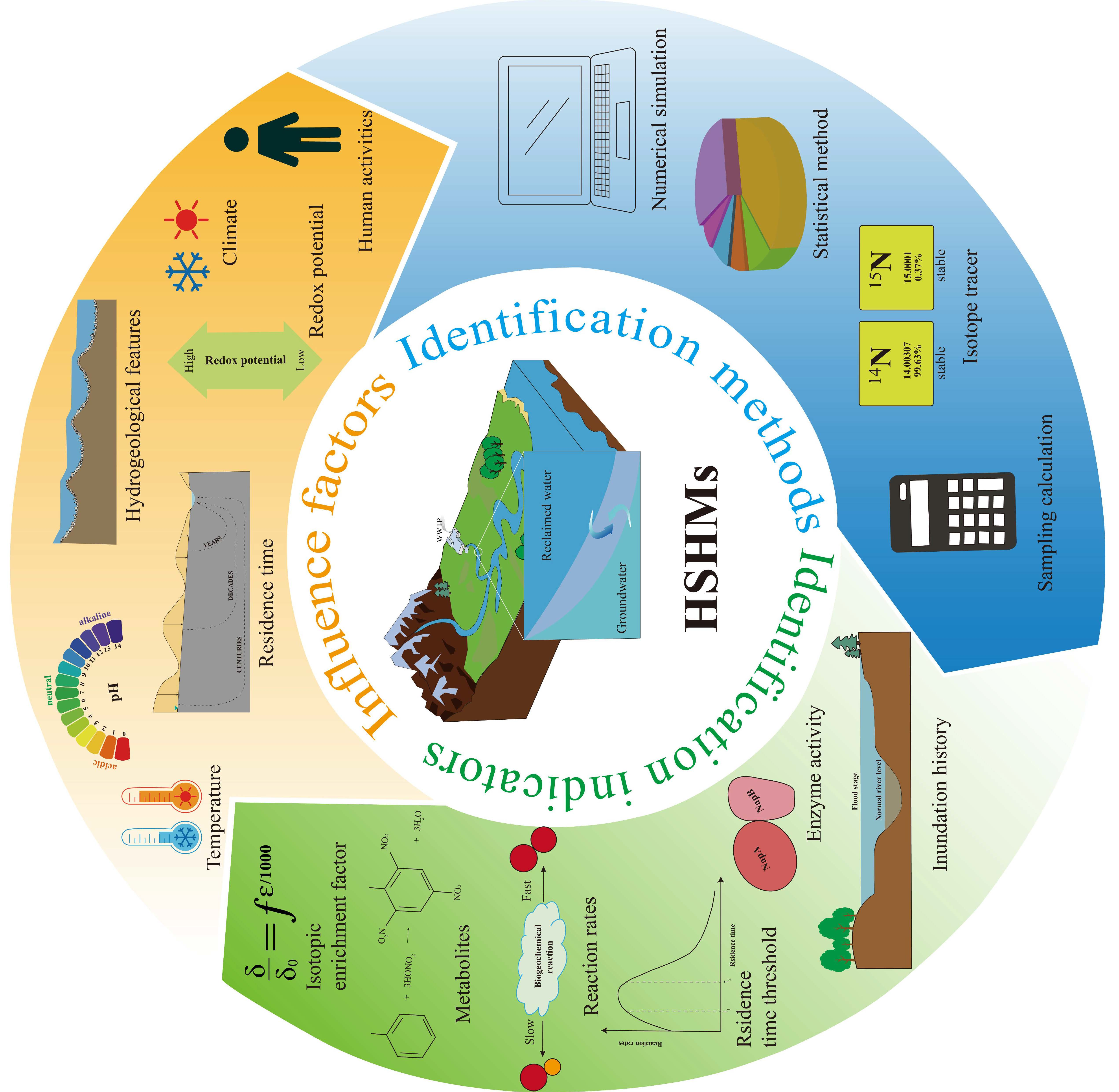
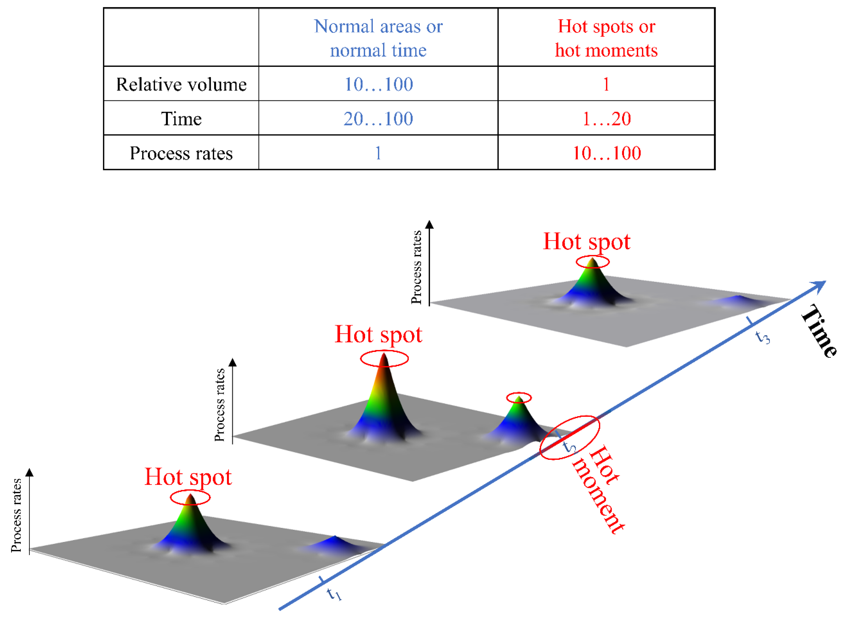
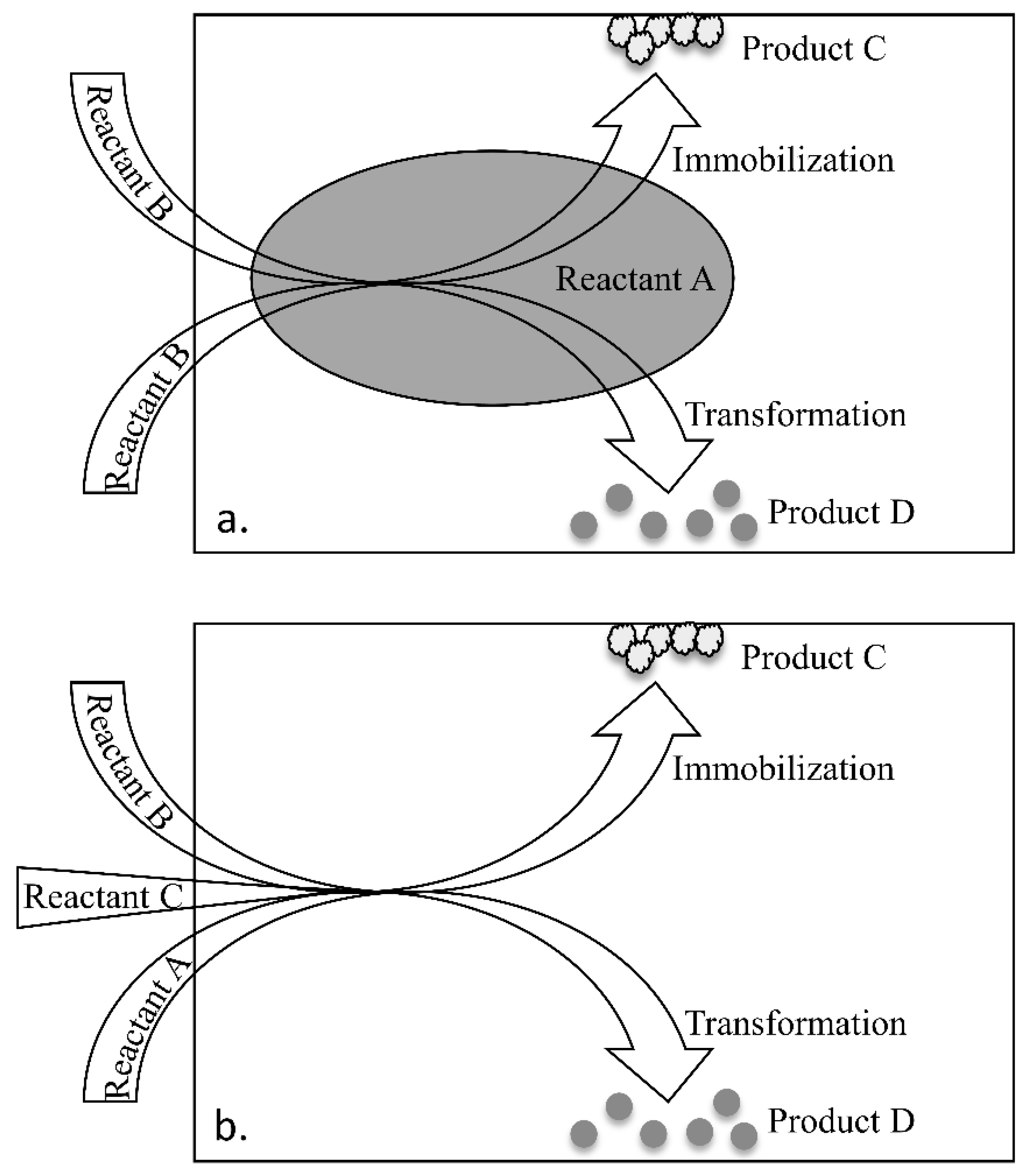
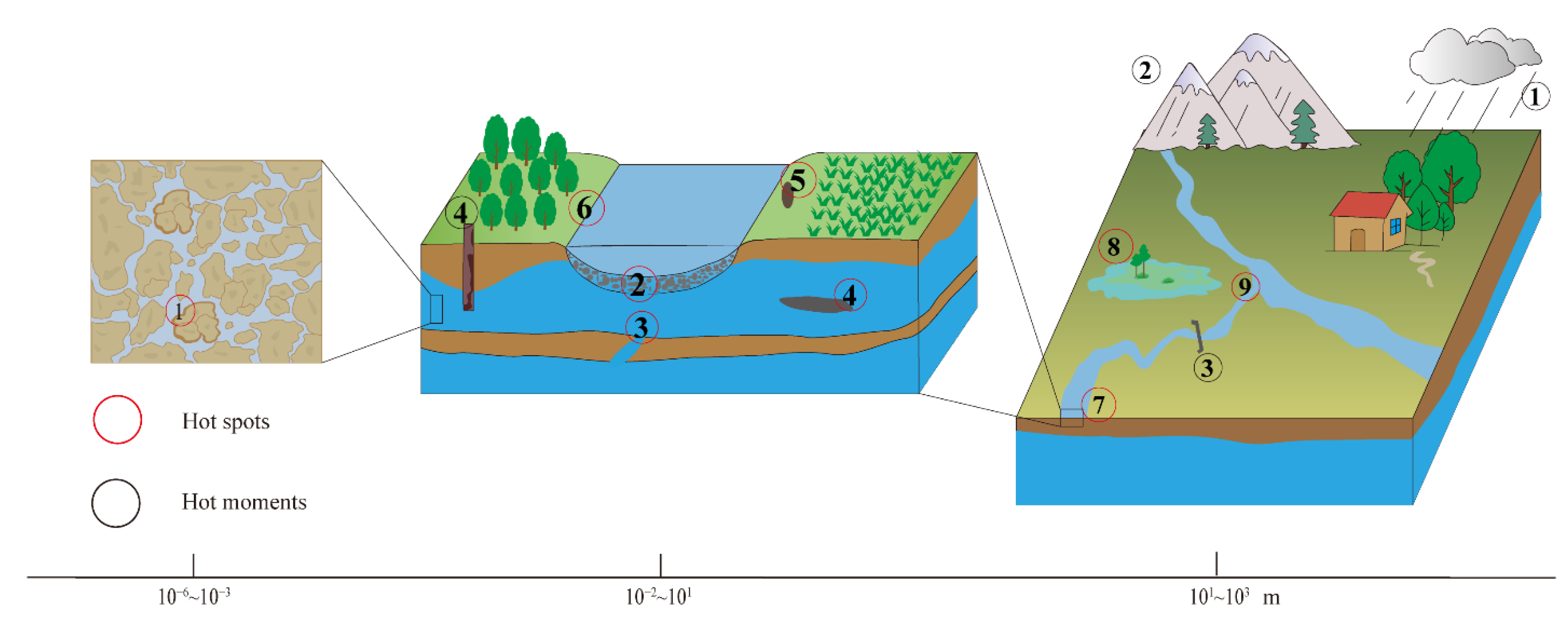
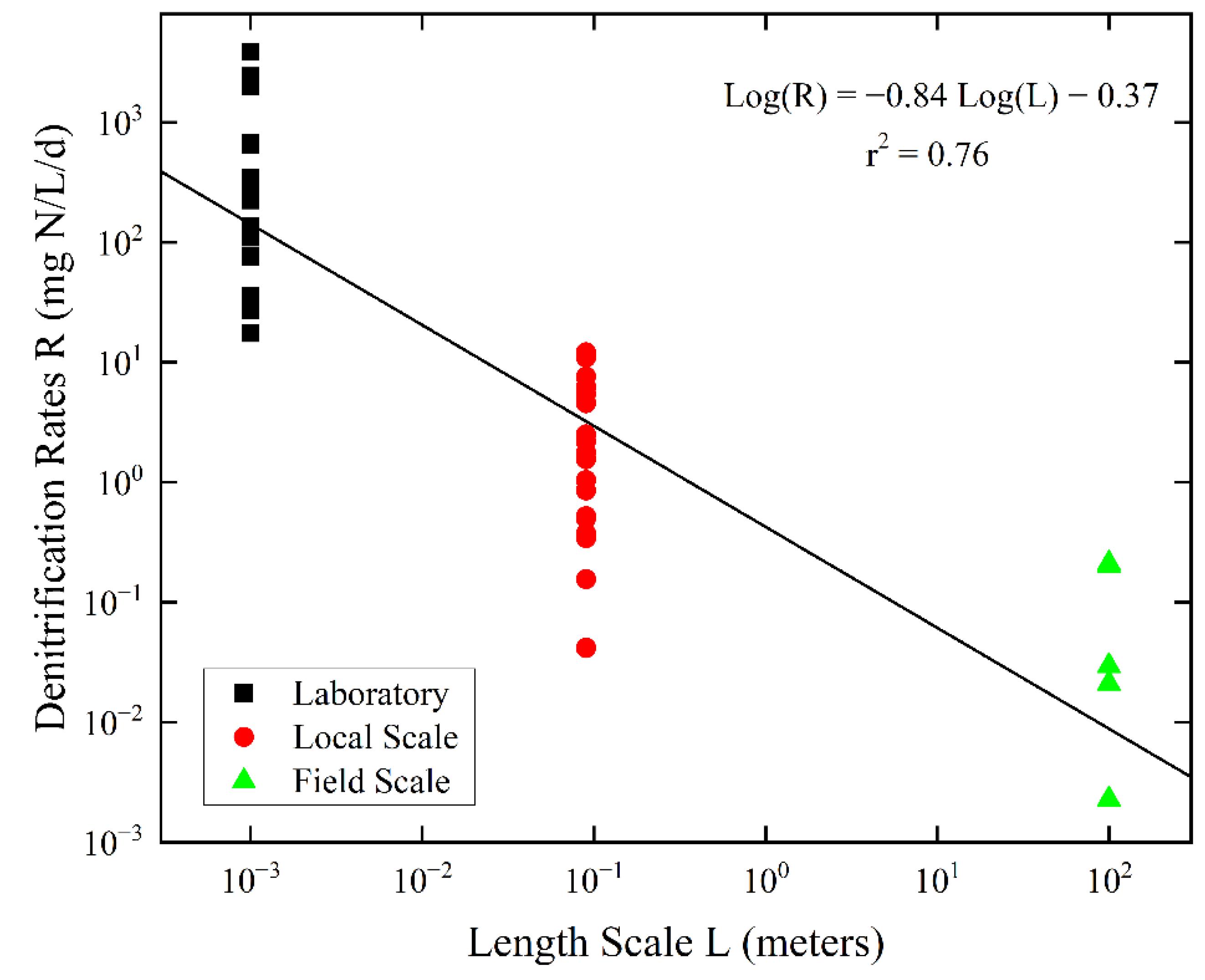
Table 1.
Comparison between the reaction rates of hot spots and conventional areas.
| Research Materials | Reaction Rates of Hot Spots | Conventional Reaction Rates | Type | References |
|---|---|---|---|---|
| N | 35 kg N ha−1 yr−1 (lab rates) | 20 kg N ha−1 yr−1 (lab rates) | HSHMs | [69] |
| N | 1.26–15.2 ug N2O-N kg soil−1 h−1 | 1.8–1.26 ug N2O-N kg soil−1 h−1 | HSHMs | [70] |
| N | 0.54 mg-N/L (the highest concentration of nitrate produced) | 0.03 mg-N/L (concentration of denitrification) | HSHMs | [71] |
| As | 738 mol (the amount of As released) | 225.6 mol (the amount of As released) | Hot spot | [56] |
| N | 17,053 nmol 15N-N2 L−1 h−1 (max) | 25 nmol 15N-N2 L−1 h−1 (min) | Hot spot | [72] |
| U (Ⅵ) | 3.5–4.5 umol/g sediment/d (max) | 0 | Hot spot | [53] |
| Hg | 7.62 ng/L (concentration of methylmercury) | Detection limit (0.06 ng/L) | Hot spot | [73] |
| N | 5.40 ug N2O L−1 min−1 | 2.91 ug N2O L−1 min−1 | Hot spot | [74] |
| N | 55,400 ng N2O-N g−1 d−1 (max) | Undetectable (min) | Hot spot | [60] |
| N | 1.9 gd−1 m−1 (max) | 0 | Hot moment | [75] |
Notes: N, nitrogen; U, uranium; Hg, mercury; As, arsenic.
Table 2.
A summary of HSHM indicators.
| Comprehensive Indicators | Specific Indicators | Applications/Substances of Concern | References | Description |
|---|---|---|---|---|
| Reaction rates | Reaction rates | Denitrification/N | [75] | Detailed field information suitable for a small scale is required during simulation. |
| Denitrification/N | [70] | Measuring reaction rates in the field is likely to miss HSHMs. | ||
| Attenuation ratio | Nitrification and denitrification/N; Biodegradation/TOC | [204]; [33] | Simple and easy to use, but not precise enough. | |
| Isotopic enrichment factor | Denitrification/N | [205] | Suitable for large-scale biogeochemical HSHM indications. | |
| Microbial community distribution or enzyme activity | Denitrifying enzyme activity/N; Microbial community distribution and bssA a/BETX b | [92]; [206] | Substantial evidence is needed to show that this index is the key to the occurrence of biogeochemical reactions. | |
| Metabolites | Microbial degradation/ BETX, PAHs c, and heterocyclic compounds | [207] | It is generally applicable to small-scale pollutants with known degradation paths. | |
| Inundation history | Flood history triggered the conversion of mercury to methylmercury/mercury | [208] | It needs unique scenes and is not universal. | |
| Isotopic and residence time threshold | Nitrification and denitrification/N | [71] | The resulting threshold may vary with temperature and surrounding water flow conditions and requires constant monitoring. | |
| Others | Magnetic susceptibility signal | Iron oxide precipitates | [209] | It is highly specific and can only identify hot spots associated with magnetic minerals and needs to be combined with complementary techniques. |
Notes: The superscript a: bssA refers to benzylsuccinate synthase genes; b: BETX refers to benzene, toluene, ethylbenzene, and xylene; c: PAH refers to polycyclic aromatic hydrocarbons.
Publisher’s Note: MDPI stays neutral with regard to jurisdictional claims in published maps and institutional affiliations. |
© 2022 by the authors. Licensee MDPI, Basel, Switzerland. This article is an open access article distributed under the terms and conditions of the Creative Commons Attribution (CC BY) license (https://creativecommons.org/licenses/by/4.0/).
Share and Cite
MDPI and ACS Style
Li, Y.; Liu, M.; Wu, X. Reclaimed Water Reuse for Groundwater Recharge: A Review of Hot Spots and Hot Moments in the Hyporheic Zone. Water 2022, 14, 1936. https://doi.org/10.3390/w14121936
AMA Style
Li Y, Liu M, Wu X. Reclaimed Water Reuse for Groundwater Recharge: A Review of Hot Spots and Hot Moments in the Hyporheic Zone. Water. 2022; 14(12):1936. https://doi.org/10.3390/w14121936
Chicago/Turabian StyleLi, Yu, Mingzhu Liu, and Xiong Wu. 2022. "Reclaimed Water Reuse for Groundwater Recharge: A Review of Hot Spots and Hot Moments in the Hyporheic Zone" Water 14, no. 12: 1936. https://doi.org/10.3390/w14121936
Note that from the first issue of 2016, this journal uses article numbers instead of page numbers. See further details here.