
Modeling of Water Distribution System Based on Ten-Minute Accuracy Remote Smart Demand Meters


1
College of Resources and Environmental Sciences, China Agricultural University, Beijing 100083, China
2
Department of Municipal Engineering, Hefei University of Technology, Hefei 230009, China
3
Hefei Water Group, Hefei 230011, China
*
Author to whom correspondence should be addressed.
Water 2022, 14(12), 1934; https://doi.org/10.3390/w14121934
Submission received: 14 May 2022
/
Revised: 12 June 2022
/
Accepted: 13 June 2022
/
Published: 16 June 2022
(This article belongs to the Section Urban Water Management)
Abstract
:In the process of water distribution system modeling, nodal demands have been deemed to be the most significant input parameters causing uncertainties. Conventionally, users of the same type are assigned the same demand pattern, which does not reflect the variability in demand patterns. In Hefei City, a lot of remote smart demand meters were installed in recent years, providing real-time water consumption data for different water user sites. In this study, the water consumption data based on 10 min accuracy were collected and used in the established EPANET model of the study area. A 48 h simulation, including workdays and weekends, was carried out, and each node’s base demand and demand pattern were accurately calculated according to the remote data. The results show that the accuracy of the model has met the modeling criteria (less than 2 m for all pressure monitoring points), and there is no need to calibrate the nodal demand. The established offline hydraulic model can better reflect the water consumption characteristics of each type of user and has revealed the significant influence of secondary water supply systems.
1. Introduction
Hydraulic models of water distribution systems (WDSs) have been increasingly applied by water utilities and researchers for various purposes, such as planning and management of systems [1] and leakage detection and location [2,3,4]. The main factors affecting the accuracy of a WDS hydraulic model are divided into two categories: deterministic parameters and uncertain parameters [5]. The deterministic parameters are the basic data of the WDS (the elevation of nodes; the material, length and diameter of pipes), whereas the uncertainty parameters mainly include the nodal demands and pipe roughness coefficients [6]. The deterministic parameters can be modified accurately according to the measured data, but the uncertainty parameters are the most uncertain input variables in a simulation model because they are not directly measurable [7,8,9]. Therefore, how to determine the nodal demands and pipe roughness coefficients more accurately, so as to improve the modeling accuracy to the greatest extent, is an urgent problem to be solved.
In the past few decades, numerous methods have been developed for the calibration of pipe roughness coefficients, such as trial-and-error or empirical methods [10,11], explicit or hydraulic simulation methods [12,13] and implicit or optimization methods [14,15,16,17,18]. At present, robust algorithms have been developed for the automatic calibration of pipe roughness coefficients and compiled in commercial software, such as WaterGEMS [19]. However, for nodal demands, because of a lack of remote demand meters in the pipe network in the past [20], the traditional two-step method is used in most cases to build an offline hydraulic model, i.e., the base demand at each node is firstly calculated based on the population served, the consumption records or engineering experience [21,22]. Then, to reduce the number of unknowns and make the problem solvable, nodes with the same type of users (residential, commercial, industrial) are grouped and assumed to have the same demand pattern in a day [23]. Although some researchers have proposed various calibration methods for the nodal demand to improve the accuracy of the offline hydraulic model, nodal demands are still deemed to be the most significant input parameters causing uncertainties [24].
In recent years, with the rapid development of the Internet of Things and 5G, a large number of smart demand meters have been used in WDSs in some cities worldwide [25]. Smart demand meters provide consumption data with high spatial and temporal resolution for all types of users [26] and enable a much better understanding of the users’ diurnal demand patterns [27]. Therefore, some scholars have explored establishing a real-time hydraulic WDS model. Machell et al. [28] established an online model using Aquis software and a SCADA system. Shafiee et al. [29] modified the core EPANET engine and combined the demand meter readings of all nodes with a WDS model to establish a dynamic real-time hydraulic model. However, compared to the offline model, the accuracy of a real-time model is affected by more factors, which will produce large errors [30]. In addition, the complex algorithms and high cost of building a real-time hydraulic model limit its applicability in cities, and many water utilities still prefer a high-accuracy off-line hydraulic model.
In this study, a high-precision offline hydraulic modeling process based on 10 min accuracy remote smart demand meters is presented. The base demand and demand pattern of each node were accurately calculated. Uncertainties caused by nodal demands were effectively resolved. Comparisons between simulated results and measured results verified that the established model meets pressure criteria. Some new findings based on the model are presented and analyzed.
2. Methodology
2.1. Study Area
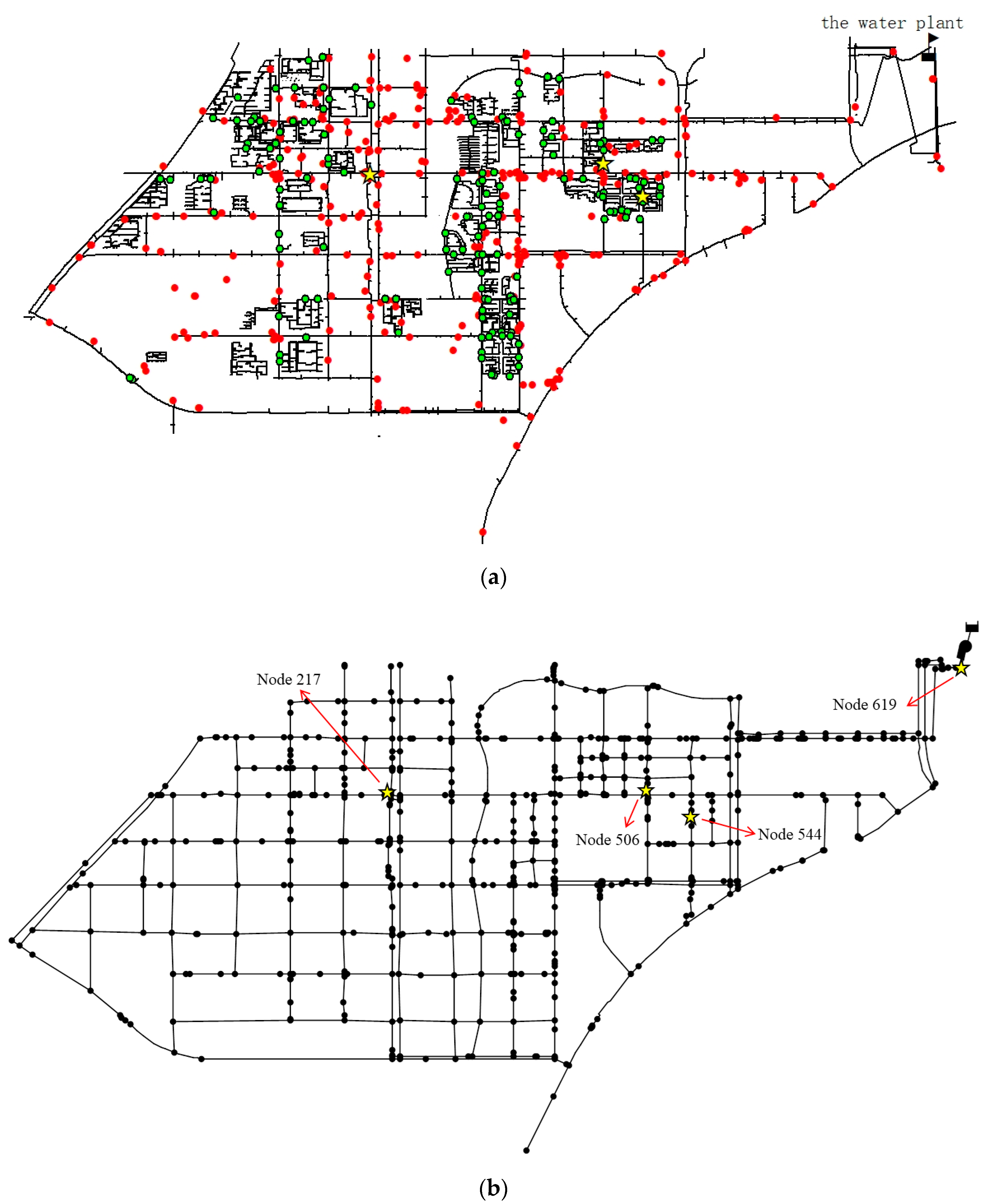
The modeling area of this study is Binhu District, Hefei City, Anhui Province, located in the middle of China. The geographical extent of the study area varies from 31.73° N, 117.24° E to 31.69° N, 117.33° E. The total modeling area is about 21.5 square kilometers. The ground elevation ranges from 9.76 m to 28.56 m. This area has a complete GIS of the WDS (see Figure 1a), which provides a basic database for the construction of the hydraulic model. Binhu District is supplied by a water plant located in the east of the area. The water plant is installed with a pressure logger and a flow meter. In addition, a large number of remote smart demand meters were installed in the area in 2018, and the time precision of measurements is 10 min, with 6 data points per hour. In Figure 1a, the green dots represent the meters for measuring the residential areas (99 m in total), and the red dots represent the meters for measuring non-resident users, including industrial users (64 m in total) and commercial users (110 m in total). In addition, three pressure loggers (with full scale of 0~1 MPa and accuracy of 1%, yellow stars in Figure 1a) were installed in the WDS to monitor the whole system, and real-time data from these three points were used for model calibration. In this study, one year of data were collected from November 2019 to November 2020.
EPANET 2.0 [31] was used for constructing the hydraulic model in this study. According to the information in the GIS, deterministic parameters of each node and each pipe were input in the model. The Hazen–William formula was chosen for calculating the frictional loss. For the initial values of the pipe roughness coefficients, the pipes with similar age, material, diameter and relative locations were assigned the same value [32,33] according to the experience value table in EPANET User’s Manual [31] (Table 1). As shown in Figure 1b, it includes a reservoir, a pump, 625 nodes and 753 pipes. Among them, 273 nodes are water consumption points, and the rest are pipeline connection points with no demands. The total length of all pipes is 118.0 km. Most pipes are made of ductile iron (91.92%), and a small part is steel (8.08%). Pipe diameters range from 200 mm to 1400 mm, and pipes with a diameter of 300 mm account for the largest proportion (73.01%). Three pressure monitoring points are numbered as Node 217, Node 506 and Node 544. The pressure logger in the water plant is numbered as Node 619.
2.2. Ten-Minute Accuracy Water Consumption Data for Different Types of Users
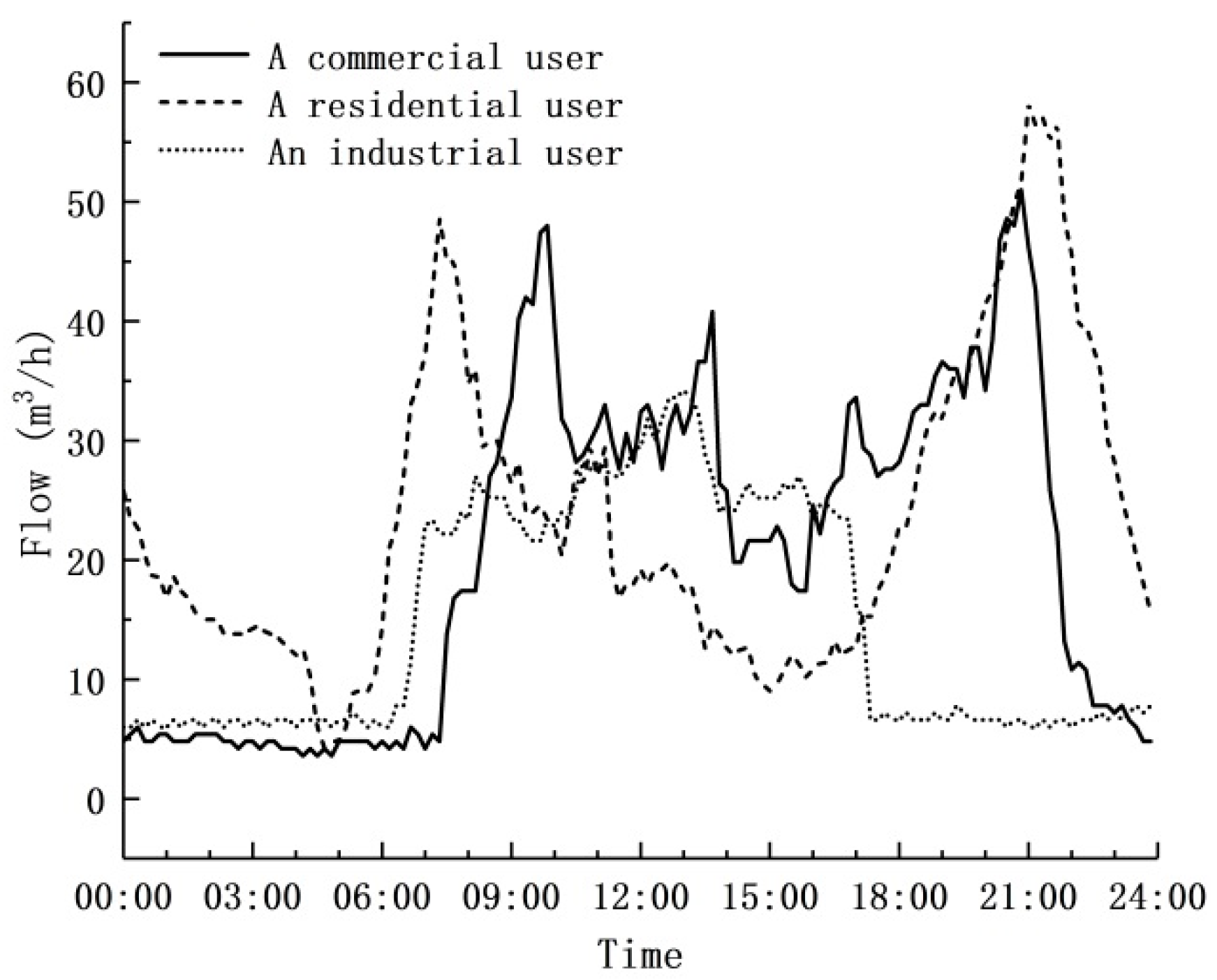
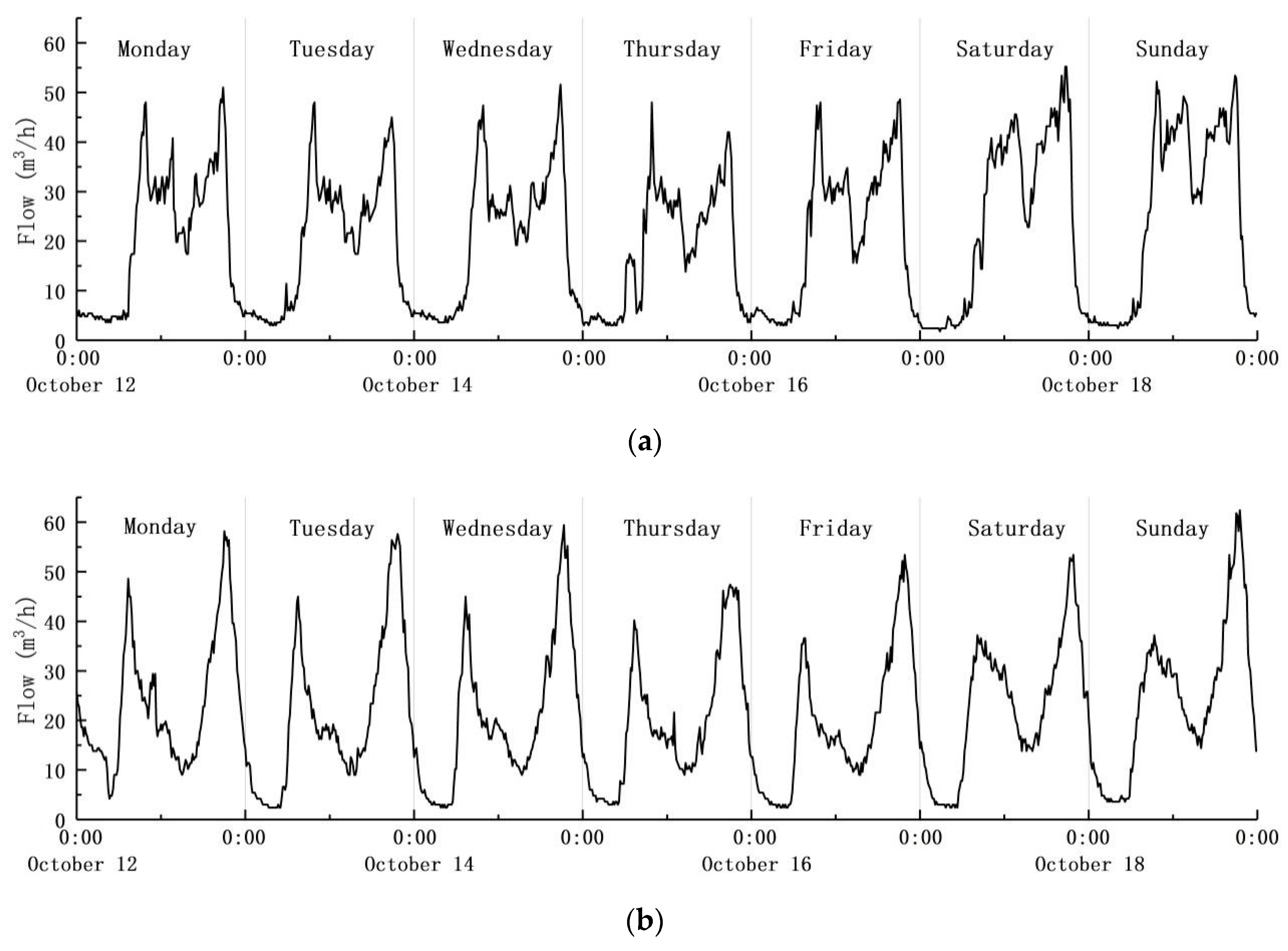
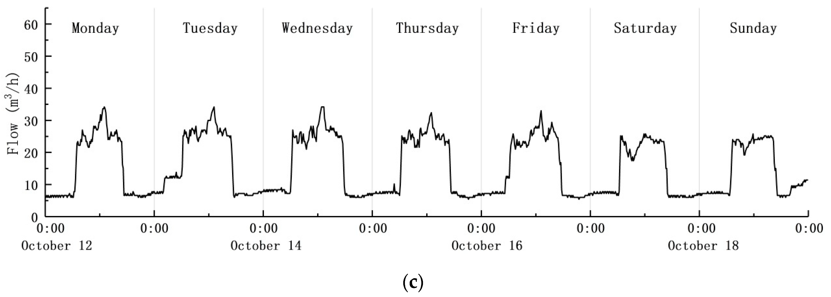
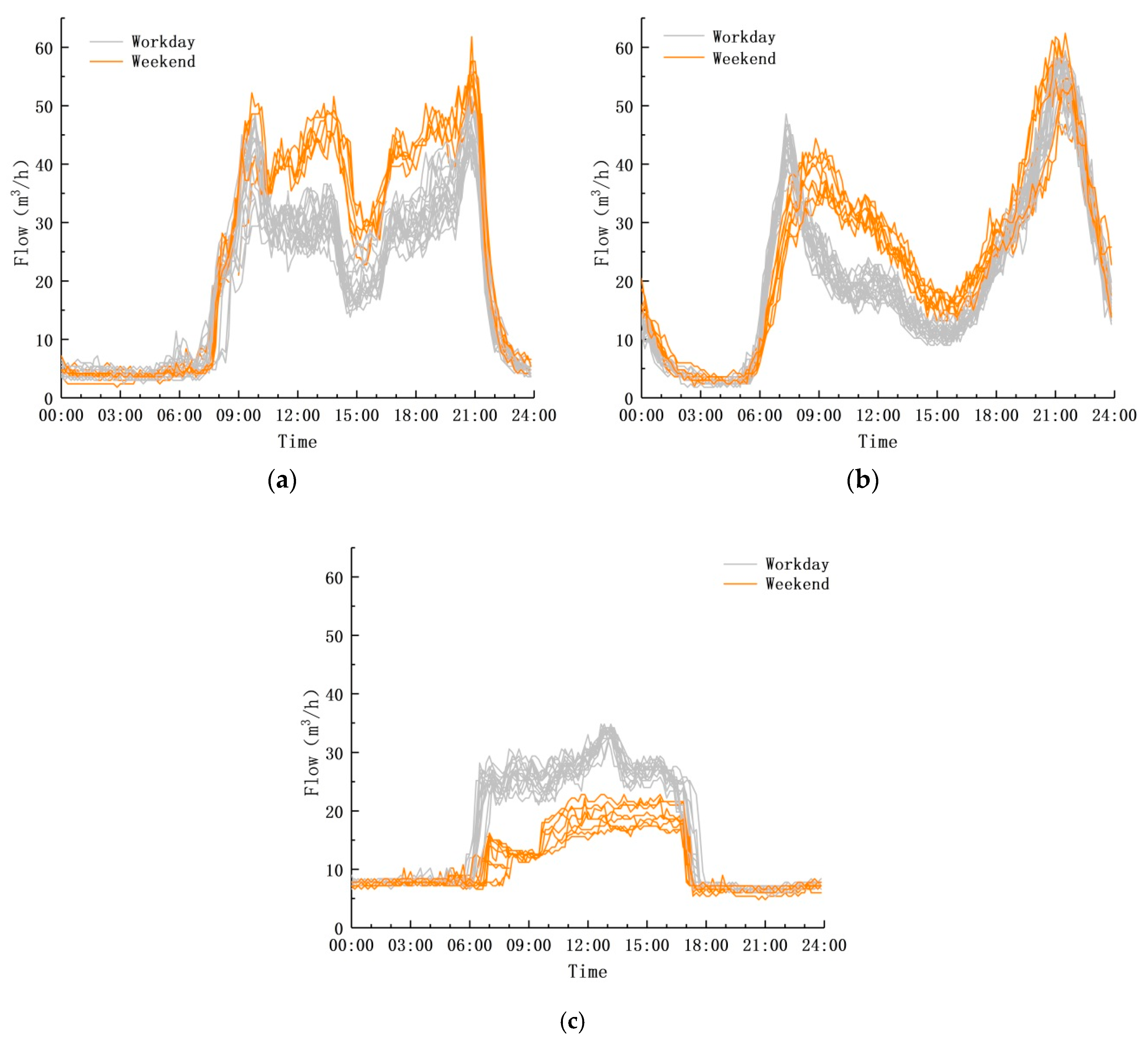
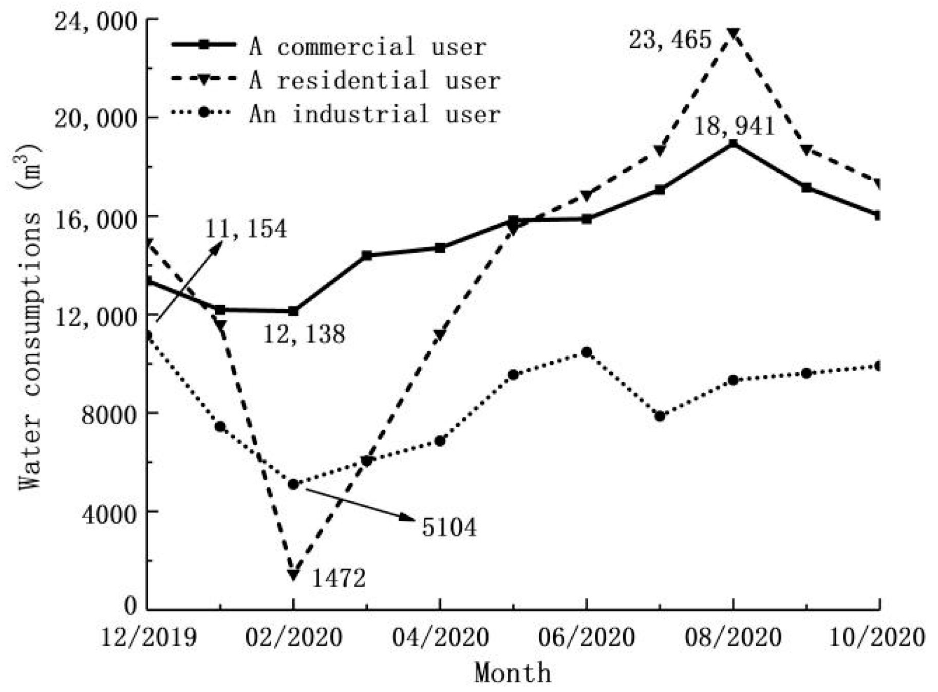
In order to better show the ten-minute accuracy water consumption data and water consumption characteristics of users, three nearby nodes within a district of the study area representing different types of users, a commercial user, a residential user and an industrial user, were selected for detailed analysis. Figure 2 shows the ten-minute accuracy water consumption curves for three types of users. Firstly, it can be seen that different types of users show very different diurnal patterns. Both the commercial and residential users have two peak times, whereas the industrial user has a relatively steady water consumption during the daytime (between 7:00 a.m. and 17:00 p.m.). Secondly, the morning peak time of the residential user happens at 7:00 a.m., while it is delayed three hours (at 10:00 a.m.) for the commercial user. To better compare the diurnal pattern of the three users, their water consumption data in one week are plotted separately in Figure 3. From Figure 3, it is firstly noticeable that the industrial user has very different diurnal patterns in one week. On workdays, from Monday to Friday, only one peak time happens, at 12:00 am, and the maximum flow is 35 m3/h. However, on Saturday and Sunday, no obvious peak time exists, and the total water consumption on the weekend is obviously less than on a workday. Actually, differences in the daily water consumption between workdays and weekends also exist for the commercial and residential users. To better show this phenomenon, daily water consumption in one month (October 2020) is plotted in Figure 4 for the three types of users. In Figure 4, black curves show workdays’ consumption in the month, while yellow curves represent the weekends’ data. Two different water demand patterns for workdays and weekends can be clearly distinguished for all three users in the figure. Therefore, to improve the accuracy of the model, it is necessary to calculate the base demand and demand pattern for both workdays and weekends. Actually, these daily, weekly and monthly water consumption patterns are closely related to local working and living characteristics. In addition, it is also easy to understand that water consumption differs greatly in different months (complete monthly data are from December 2019 to October 2020), as shown in Figure 5. For the residential user, the minimum water consumption happens in February, and the maximum consumption happens in August. The ratio of the maximum value to the minimum value is 1.56. For the industrial user, the minimum water consumption happens in February, and the maximum consumption happens in December. The ratio of the maximum value to the minimum value is 2.19. However, for the commercial user, the total water consumption in August reaches as much as 15.94 times the value for February. Considering that the base demand of each user varies from month to month, to improve the accuracy of the model, the base demand and demand pattern of each node should be updated every month.
Based on the ten-minute accuracy data, the base demand and demand pattern of each node for every day, week and year can be calculated. However, from the above analysis, it is found that the daily water consumption pattern only differs greatly between workdays and weekends and among months. To reduce the data processing and modeling time, it is reasonable to calculate the monthly averaged base demand and demand pattern for workdays and weekends for each node and input the results into the EPANET hydraulic model of the study area. To achieve this, the calculation method of the monthly averaged base demand and demand pattern is explained in the next section.
2.3. Calculation Method of Monthly Averaged Base Demand and Demand Pattern
According to the data of the remote smart demand meter corresponding to each node, the monthly averaged base demand and demand pattern at each node were calculated by the water consumption curve method. The basic steps are given below:
- 1.
- Hourly average water consumption in a month: according to the remote flow data of node i, the water consumption in each hour t in the 24 h period in each day in a month was summed up and then divided by the total number of days in the month (workdays and weekends are calculated, respectively):where qi,t is the hourly average water consumption (m3/h) of node i in tth hour of a day, t = 1, 2, 3…24; is the water consumption (m3/h) in jth day in tth hour of the node i; and N represents total days in a month.
- 2.
- Base demand at each node: The hourly average water consumption at each hour was added up and then divided by 24:where qi is the base demand of node i (m3/h).
- 3.
- Hourly variation coefficients: The ratio of hourly average water consumption in tth hour to the base demand is the hourly variation coefficient:where Xi,t is the hourly variation coefficient of node i in tth hour, and it is a fixed value in each hour.
- 4.
- Demand pattern input: Taking time as abscissa and Xi,t as ordinate, then the demand pattern at node i can be input. A 48 h simulation (a 24 h simulation for the workday and a 24 h simulation for the weekend) was proposed and conducted.
3. Results and Discussions
3.1. Comparison between Simulation and Measured Pressures
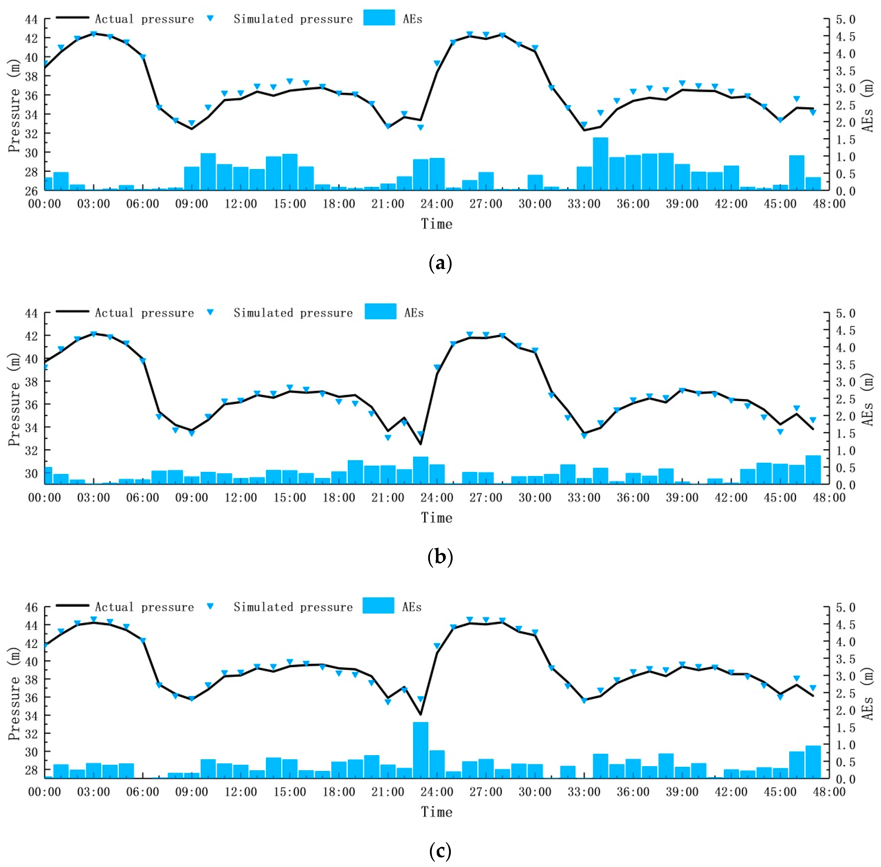
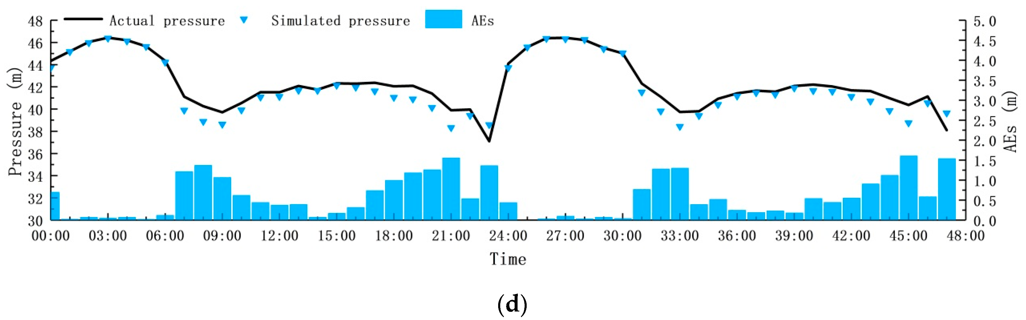
There are four pressure monitoring points in the WDS (Node 217, Node 506, Node 544 and Node 619, as shown in Figure 1b), and comparisons between simulated pressures and the actual pressures at these points are shown in Figure 6. It can be seen that the simulated results and the measured results show very good agreement, with the absolute errors (AEs) being less than 2 m for all nodes. Actually, in most instances, the AEs are within 1 m, with the largest value being 1.64 m (at Node 544 at 23:00). Node 506 obtains the best simulation results, with the AEs being less than 1 m for every hour (the largest value is 0.83 m happening at 23:00). Node 619 shows relatively worse results, with the AEs at 12 h being greater than 1 m. This is because Node 619 is located in the water plant, and its operating pressure is greater than the other three nodes. The model has already met the modeling criteria (±2 m for all monitoring points) specified by the Water Research Centre [34], so there is no need to calibrate the nodal demands. In order to further improve the accuracy of the model, only the pipe roughness coefficients need to be calibrated, which reduces the time and complexity of the calibration.
The Darwin calibrator in WaterGEMS software is selected to calibrate the pipe roughness coefficients, which uses a genetic algorithm (GA) as the optimization tool. The objective function is defined as the minimization of squared differences between actual and simulated values of pressure at monitoring points in WDS by adjusting the pipe roughness coefficients. It can be written as Equation (4):
where F is objective function to be minimized; and are the actual pressure and simulated pressure at node i in tth time period, respectively; NH is the number of pressure loggers installed in the network; T is the simulation time periods of calibration. For the accuracy of the model, the pressure observations of 48 h (including a workday and a weekend day) are all used for the simultaneous calibration of pipe roughness coefficients.
To ensure the calibrated values are practically meaningful, it is necessary to ensure the values of pipe roughness coefficients are within the specified ranges, as shown in Equation (5):
where Cj,initial is the initial value of roughness at pipe j; cmin and cmax are the minimum and maximum adjustment coefficients of pipe roughness coefficients, respectively. In the paper, the adjustment coefficients are given as cmin = 0.85 and cmax = 1.15.
Before and after calibration, the number of time periods (48 in total) in each AE section is shown in Table 2. First of all, it can be seen that because Node 619 is the outlet node of the water plant, it will not be affected when the pipe roughness coefficients are changed. For the other three nodes, it can be clearly seen that after calibration, the AEs of all time periods are less than 1.5 m. There are only three time periods in which the AEs are greater than 1 m. After calibration, the maximum AEs of the three nodes (Node 217, Node 506 and Node 544) are 1.44 m, 0.85 m and 1.36 m, respectively. The accuracy of the model is further improved by the calibration of pipe roughness coefficients, which can better reflect the actual operation and hydraulic characteristics of the pipe network.
3.2. Advantages of the Established High-Accuracy Offline Hydraulic Model
Through the analysis in Section 3.1, it can be seen that the model established based on smart demand meters has high accuracy, and the calibration method is simple. It is believed that the more reasonable and more accurate nodal demand input parameters have significantly reduced model uncertainties. In the traditional two-step method for building the offline hydraulic model, users with the same type are usually grouped and assigned the same base demand and demand pattern. Although this has inevitably caused great errors in the model, it has been balanced by continually calibrating the pipes’ roughness coefficients. The established hydraulic model based on the ten-minute accuracy data from the smart meters allows us to conduct detailed error analysis on demand patterns of users of the same type. Figure 7 shows the 48 h demand pattern curves of the three types of users. For the two commercial users in Figure 7a, although the 48 h variation coefficient curves generally show similarity, the peak demand times have obvious differences both during the workday and on the weekend. This situation also applies to the two industrial users in Figure 7c. However, in Figure 7b, it is surprising to see totally different water demand patterns for the two residential users. The peak demand time for residential user A happens at 7:00 in the morning and at 21:00 in the night, which is consistent with normal residential users’ demand patterns. However, for residential user B, the peak time happens at 4:00 in the morning and at around 16:00 in the afternoon. Communication with the municipal manager revealed that a secondary water supply system is used at the location of residential user B. The second water supply tank takes and stores water from the network during off-peak periods, while it supplies water to the network to balance peak hours’ demands. This explains the nearly reversed demand pattern curves between the two users. Furthermore, it was later found that a lot of secondary water supply systems are in use in the network to better balance the water demand and pressure in the whole network [35]. Based on the established hydraulic model, the significant influences of secondary water supply systems on the demand patterns of residential users have been revealed, which has never been reported in previous studies.
4. Conclusions
In this paper, an applicable method for how to reduce uncertainties in a WDS model caused by the nodal demands was proposed. A high-accuracy offline hydraulic model of WDS in Binhu District of Hefei City in Anhui Province was established by using EPANET 2.0 based on data collected from 10 min accuracy remote smart demand meters. Firstly, the base demands and demand patterns of all nodes were accurately calculated, using monthly average data, by the water consumption curve method. Then, a total of 48 h of simulation were conducted, including workdays and the weekend. Compared to the measured pressures, the AEs at all pressure monitoring points were less than 2 m during simulation time, and there is no need to calibrate the nodal demand. The Darwin calibrator in WaterGEMS software was used to calibrate the pipe roughness coefficients and has further improved the model’s accuracy. Based on the model, the significant influences of secondary water supply systems on the network have been noticed and revealed for the first time. In addition, more pressure monitoring points are currently being installed in the network, and more data will be collected for comparison and calibration in the future.
Author Contributions
Conceptualization, S.G.; methodology, R.S. and S.G.; software, X.L.; data resources, B.Z.; writing, R.S. and X.L. All authors have read and agreed to the published version of the manuscript.
Funding
This work was supported by the National Science Foundation of Anhui Province (grant number: 1908085QE211; Funder: Anhui Provincial Department of Science and Technology) and the Key Research and Development Program in Anhui Province (grant number: 202104i07020012; 1; Funder: Anhui Provincial Department of Science and Technology).
Institutional Review Board Statement
Not applicable.
Informed Consent Statement
Not applicable.
Data Availability Statement
The data presented in this study are available on request from the corresponding author. The data are not publicly available due to due to conditions of the ethics committee of our university.
Conflicts of Interest
The authors declare no conflict of interest.
References
- Marsili, V.; Meniconi, S.; Alvisi, S.; Brunone, B.; Franchini, M. Stochastic approach for the analysis of demand induced transients in real water distribution systems. J. Water Res. Plan. Manag. 2022, 148, 04021093. [Google Scholar] [CrossRef]
- Kang, D.; Lansey, K. Novel approach to detecting pipe bursts in water distribution networks. J. Water Res. Plan. Manag. 2014, 140, 121–127. [Google Scholar] [CrossRef]
- Tao, T.; Huang, H.; Li, F.; Xin, K. Burst detection using an artificial immune network in water-distribution systems. J. Water Res. Plan. Manag. 2014, 140, 04014027. [Google Scholar] [CrossRef]
- Meniconi, S.; Brunone, B.; Frisinghelli, M. On the role of minor branches, energy dissipation, and small defects in the transient response of transmission mains. Water 2018, 10, 187. [Google Scholar] [CrossRef] [Green Version]
- Alvisi, S.; Franchini, M. Pipe roughness calibration in water distribution systems using grey numbers. J. Hydroinform. 2010, 12, 424–445. [Google Scholar] [CrossRef] [Green Version]
- Do, N.C.; Simpson, A.R.; Deuerlein, J.W.; Piller, O. Calibration of water demand multipliers in water distribution systems using genetic algorithms. J. Water Res. Plan. Manag. 2016, 142, 04016044. [Google Scholar] [CrossRef]
- Kang, D.; Lansey, K. Demand and roughness estimation in water distribution syste-ms. J. Water Res. Plan. Manag. 2011, 137, 20–30. [Google Scholar] [CrossRef]
- Zanfei, A.; Menapace, A.; Santopietro, S.; Righetti, M. Calibration procedure for water distribution systems: Comparison among hydraulic models. Water 2020, 12, 1421. [Google Scholar] [CrossRef]
- Du, K.; Long, T.-Y.; Wang, J.-H.; Guo, J.-S. Inversion model of water distribution systems for nodal demand calibration. J. Water Res. Plan. Manag. 2015, 141, 04015002. [Google Scholar] [CrossRef]
- Walski, T.M. Case study: Pipe network model calibration issues. J. Water Res. Plan. Manag. 1986, 112, 238–249. [Google Scholar] [CrossRef]
- Bhave, P.R. Calibrating water distribution network models. J. Environ. Eng. 1988, 114, 120–136. [Google Scholar] [CrossRef]
- Ormsbee, L.E.; Wood, D.J. Explicit pipe network calibration. J. Water Res. Plan. Manag. 1986, 112, 166–182. [Google Scholar] [CrossRef]
- Boulos, P.F.; Wood, D.J. Explicit calculation of pipe-network parameters. J. Hydraul. Eng. 1990, 116, 1329–1344. [Google Scholar] [CrossRef]
- Ormsbee, L.E. Implicit network calibration. J. Water Res. Plan. Manag. 1989, 115, 243–257. [Google Scholar] [CrossRef]
- Savic, D.A.; Walters, G.A. Genetic Algorithm Techniques for Calibrating Network Models; Rep. No. 95/12; Centre for Systems and Control Engineering, University of Exeter: Exeter, UK, 1995. [Google Scholar]
- Kapelan, Z.S.; Savic, D.A.; Walters, G.A. Calibration of water distribution hydra-ulic models using a Bayesian-type procedure. J. Hydraul. Eng. 2007, 133, 927–936. [Google Scholar] [CrossRef]
- Walski, T.M.; DeFrank, N.; Voglino, T.; Wood, R.; Whitman, B.E. Determining the accuracy of automated calibration of pipe network models. In Proceedings of the 8th Annual Water Distribution Systems Analysis Symposium, (CD-ROM), Cincinnati, OH, USA, 27–30 August 2006; ASCE: Reston, VA, USA, 2008. [Google Scholar]
- Koppel, T.; Vassiljev, A. Calibration of a model of an operational water distribution system containing pipes of different age. Adv. Eng. Softw. 2009, 40, 659–664. [Google Scholar] [CrossRef]
- Mentes, A.; Galiatsatou, P.; Spyrou, D.; Samaras, A.; Stournara, P. Hydraulic simulation and analysis of an urban center’s aqueducts using emergency scenarios for network operation: The case of Thessaloniki City in Greece. Water 2020, 12, 1627. [Google Scholar] [CrossRef]
- Lawrence, L.; Yskandar, H.; Adnan, A.M. Estimation of water demand in water distribution systems using particle swarm optimization. Water 2017, 9, 593. [Google Scholar] [CrossRef] [Green Version]
- Kang, D.; Lansey, K. Real-time demand estimation and confidence limit analysis for water distribution systems. J. Hydraul. Eng. 2009, 135, 825–837. [Google Scholar] [CrossRef]
- Zhang, Q.; Zheng, F.; Duan, H.F.; Jia, Y.; Zhang, T.; Guo, X. Efficient numerical approach for simultaneous calibration of pipe roughness coefficients and nodal demands for water distribution systems. J. Water Res. Plan. Manag. 2018, 144, 04018063. [Google Scholar] [CrossRef]
- Jung, D.; Choi, Y.H.; Kim, J.H. Optimal node grouping for water distribution system demand estimation. Water 2016, 8, 160. [Google Scholar] [CrossRef] [Green Version]
- Pasha, M.; Lansey, K. Analysis of uncertainty on water distribution hydraulics and water quality. In Proceedings of the World Water and Environmental Resources Congress, Anchorage, AK, USA, 15–19 May 2005; pp. 1–12. [Google Scholar] [CrossRef]
- Creaco, E.; Campisano, A.; Fontana, N.; Marini, G.; Page, P.R.; Walski, T. Real time control of water distribution networks: A state-of-the-art review. Water Res. 2019, 161, 517–530. [Google Scholar] [CrossRef] [PubMed]
- Zhang, Q.; Zheng, F.; Jia, Y.; Savic, D.; Kapelan, Z. Real-time foul sewer hydraulic modelling driven by water consumption data from water distribution systems. Water Res. 2021, 188, 116544. [Google Scholar] [CrossRef] [PubMed]
- Marsili, V.; Meniconi, S.; Alvisi, S.; Brunone, B.; Franchini, M. Experimental analysis of the water consumption effect on the dynamic behaviour of a real pipe network. J. Hydraul. Res. 2021, 59, 477–487. [Google Scholar] [CrossRef]
- Machell, J.; Mounce, S.R.; Boxall, J.B. Online modelling of water distribution systems: A UK case study. Drink. Water Eng. Sci. 2010, 3, 21–27. [Google Scholar] [CrossRef]
- Shafiee, M.E.; Rasekh, A.; Sela, L.; Preis, A. Streaming smart meter data integration to enable dynamic demand assignment for real-time hydraulic simulation. J. Water Res. Plan. Manag. 2020, 146, 06020008. [Google Scholar] [CrossRef]
- Shafiee, M.E.; Barker, Z.; Rasekh, A. Enhancing water system models by integrating big data. Sustain. Cities Soc. 2017, 37, 485–491. [Google Scholar] [CrossRef]
- Rossman, L.A. EPANET 2: Users’ Manual; National Risk Management Research Laboratory, Office of Research and Development, United Sates Environmental Protection Agency (EPA): Cincinnati, OH, USA, 2000. [Google Scholar]
- Kumar, S.M.; Narasimhan, S.; Bhallamudi, S.M. Parameter estimation in water distribution networks. Water Res. Manag. 2010, 24, 1251–1272. [Google Scholar] [CrossRef]
- Dini, M.; Tabesh, M. A new method for simultaneous calibration of demand pattern and Hazen-Williams coefficients in water distribution systems. Water Resour. Manag. 2014, 28, 2021–2034. [Google Scholar] [CrossRef] [Green Version]
- WRC (Water Research Centre). Network Analysis—A Code of Practice; Water Research Centre: Swindon, UK, 1989. [Google Scholar]
- Xu, Q.; Chen, Q.; Qi, S.; Cai, D. Improving water and energy metabolism efficiency in urban water supply system through pressure stabilization by optimal operation on water tanks. Ecol. Inform. 2015, 26, 111–116. [Google Scholar] [CrossRef]
Figure 1.
Study area: (a) GIS map; (b) the established EPANET model.

Figure 2.
Ten-minute accuracy water consumption curves for three types of users.

Figure 3.
Ten-minute accuracy of water consumption curves of three users in a week: (a) a commercial user; (b) a residential user; (c) an industrial user.
Figure 3.
Ten-minute accuracy of water consumption curves of three users in a week: (a) a commercial user; (b) a residential user; (c) an industrial user.


Figure 4.
Water consumption curves in a month: (a) a commercial user; (b) a residential user; (c) an industrial user.
Figure 4.
Water consumption curves in a month: (a) a commercial user; (b) a residential user; (c) an industrial user.

Figure 5.
Comparison of total water consumption in different months.

Figure 6.
Comparisons of actual pressures and simulated pressures at four points: (a) Node 217; (b) Node 506; (c) Node 544; (d) Node 619.
Figure 6.
Comparisons of actual pressures and simulated pressures at four points: (a) Node 217; (b) Node 506; (c) Node 544; (d) Node 619.


Figure 7.
Demand patterns of users of the same type: (a) two commercial users; (b) two residential users; (c) two industrial users.
Figure 7.
Demand patterns of users of the same type: (a) two commercial users; (b) two residential users; (c) two industrial users.


Table 1.
Initial values of the pipe roughness coefficient [30].
Table 1.
Initial values of the pipe roughness coefficient [30].
| Condition | Node Number | Diameter (mm) | |||
|---|---|---|---|---|---|
| 200–300 | 300–600 | 600–1000 | >1000 | ||
| Ductile iron pipe | New pipe | 140 | |||
| Five years | 125 | 130 | 135 | 135 | |
| Ten years | 115 | 120 | 130 | 130 | |
| Twenty years | 105 | 110 | 120 | 120 | |
| Steel pipe | New pipe | 120 | |||
| Five years | 115 | ||||
| Ten years | 110 | ||||
| Twenty years | 105 | ||||
Table 2.
The number of time periods in each AEs section before and after calibration.
| Condition | Node Number | The Range of AEs (m) | Maximum (mH2O) | ||||
|---|---|---|---|---|---|---|---|
| 0–0.5 | 0.5–1 | 1–1.5 | 1.5–2 | >2 | |||
| Before calibration | Node 217 | 25 | 16 | 6 | 1 | 0 | 1.53 |
| Node 506 | 38 | 10 | 0 | 0 | 0 | 0.83 | |
| Node 544 | 35 | 12 | 0 | 1 | 0 | 1.64 | |
| Node 619 | 25 | 11 | 10 | 2 | 0 | 1.61 | |
| After calibration | Node 217 | 35 | 11 | 2 | 0 | 0 | 1.44 |
| Node 506 | 34 | 14 | 0 | 0 | 0 | 0.85 | |
| Node 544 | 34 | 13 | 1 | 0 | 0 | 1.36 | |
| Node 619 | 25 | 11 | 9 | 3 | 0 | 1.61 | |
Publisher’s Note: MDPI stays neutral with regard to jurisdictional claims in published maps and institutional affiliations. |
© 2022 by the authors. Licensee MDPI, Basel, Switzerland. This article is an open access article distributed under the terms and conditions of the Creative Commons Attribution (CC BY) license (https://creativecommons.org/licenses/by/4.0/).
Share and Cite
MDPI and ACS Style
Song, R.; Liu, X.; Zhu, B.; Guo, S. Modeling of Water Distribution System Based on Ten-Minute Accuracy Remote Smart Demand Meters. Water 2022, 14, 1934. https://doi.org/10.3390/w14121934
AMA Style
Song R, Liu X, Zhu B, Guo S. Modeling of Water Distribution System Based on Ten-Minute Accuracy Remote Smart Demand Meters. Water. 2022; 14(12):1934. https://doi.org/10.3390/w14121934
Chicago/Turabian StyleSong, Ruiping, Xinyue Liu, Bo Zhu, and Shuai Guo. 2022. "Modeling of Water Distribution System Based on Ten-Minute Accuracy Remote Smart Demand Meters" Water 14, no. 12: 1934. https://doi.org/10.3390/w14121934
Note that from the first issue of 2016, this journal uses article numbers instead of page numbers. See further details here.