
Use of Multi-Criteria Decision Analysis (MCDA) for Mapping Erosion Potential in Gulf of Mexico Watersheds


1
Geosystems Research Institute, Mississippi State University, Starkville, MS 39762, USA
2
Department of Geosciences, Mississippi State University, Starkville, MS 39762, USA
*
Author to whom correspondence should be addressed.
Water 2022, 14(12), 1923; https://doi.org/10.3390/w14121923
Submission received: 15 April 2022
/
Revised: 8 June 2022
/
Accepted: 13 June 2022
/
Published: 15 June 2022
(This article belongs to the Special Issue Recent Advances in Soil Erosion and Sedimentation: From the Hillslope to Watershed)
Abstract
:The evaluation of soil erosion is often assessed using traditional soil-loss models such as the Revised Universal Soil-Loss Equation (RUSLE) and the Soil and Water Assessment Tool (SWAT). These models provide quantitative outputs for sediment yield and are often integrated with geographic information systems (GIS). The work described here is focused on transitioning towards a qualitative assessment of erosion potential using Multi-Criteria Decision Analysis (MCDA), for improved decision-support and watershed-management prioritization in a northern Gulf of Mexico coastal watershed. The foundation of this work conceptually defined watershed erosion potential based on terrain slope, geomorphology, land cover, and soil erodibility (as defined by the soil K-factor) with precipitation as a driver. These criteria were evaluated using a weighted linear combination (WLC) model to map generalized erosion potential. The sensitivity of individual criteria was accessed with the one-at-a-time (OAT) method, which simply removed one criterion and re-evaluated erosion potential. The soil erodibility and slope were found to have the most influence on erosion-potential modeling. Expert input was added through MCDA using the Analytical Hierarchy Process (AHP). The AHP allows for experts to rank criteria, providing a quantitative metric (weight) for the qualitative data. The individual AHP weights were altered in one-percent increments to help identify areas of alignment or commonality in erosion potential across the drainage basin. These areas were used to identify outliers and to develop an analysis mask for watershed management area prioritization. A comparison of the WLC, AHP, ensembled model (average of WLC and AHP models), and SWAT output data resulted in visual geographic alignment between the WLC and AHP erosion-potential output with the SWAT sediment-yield output. These observations yielded similar results between the qualitative and quantitative erosion-potential assessment approaches, with alignment in the upper and lower ranks of the mapped erosion potentials and sediment yields. The MCDA, using the AHP and ensembled modeling for mapping watershed potential, provided the advantage of more quickly mapping erosion potential in coastal watersheds for improved management of the environmental resources linked to erosion.
1. Introduction
Sediment is the largest volumetric nonpoint-source pollutant to surface waters [1,2,3] and one of the most important water-quality problems in the United States [4,5,6]. Upland watershed erosion is a serious issue for estuaries and the coastal region of the southeastern United States. During precipitation events, overland and streambank erosion increases in the watershed, often resulting in degradation to downstream resources in the associated estuary. Erosive rates are amplified in areas experiencing active land use changes with agriculture, and increasing urbanization and industrialization [7,8]. The influence of the growing human population and unrestricted development in coastal watersheds is proving to be very detrimental to the overall integrity of the fragile, yet highly productive estuarine ecosystems. This growth and development have increased pollution inputs, loss of habitat, and nutrients, and has led to degraded ecologic conditions [1,2,3]. These trends of degraded conditions due to human influence will continue to impact estuaries, creating higher instances of eutrophication, hypoxia, and anoxia.
Coastal watersheds and their estuaries are important to the overall coastal environment, and are areas of high biologic productivity [9,10]. The high level of productivity is, in part, due to the transition zone created by the mixing of the upland drainage of fresh water with saline seawater; these areas are referred to as the nurseries of the sea [11].
Modeling erosion in coastal watersheds is a complex task that involves a wide range of knowledge from several scientific and engineering disciplines. An effective understanding of coastal watersheds requires several inputs, such as coupling landscape characterization and hydrologic processes [12,13]. Developments in geographic information systems (GIS) and other geospatial technologies have greatly increased the quality and quantity of data available for hydrologic modeling [13,14,15,16]. The coupling of GIS with other models is an approach that is effective in the management of the resources of coastal watersheds. Numerous hydrologic, soil-erosion, and landscape-characterization models can couple with geospatial technologies such as GIS for improved data processing, analysis, and visualization [13,14,15,16,17].
The design of soil-erosion models allows them to work in conjunction with GIS and other geospatial applications. Examples include the Water Erosion Prediction Project (WEPP), Soil and Water Assessment Tool (SWAT), and the open-source version of the Nonpoint Source Pollution and Erosion Comparison Tool (OpenNSPECT). These models are often described as traditional soil-loss models and are either mechanistic (i.e., SWAT) or empirical, such as the Revised Universal Soil-Loss Equation (RUSLE) and Modified Soil-Loss Equation [18]. Soil erosion across the landscape has traditionally been characterized using models such as the RUSLE [19,20] and the WEPP [21,22,23]. The combination of many of these models with GIS helps with the transition from models to decision-support and analysis. Modeling approaches are typically either classified as qualitative or quantitative [24]. A quantitative model is data driven, and it is difficult to apply this model in data-poor regions. Additionally, a quantitative model is not enough to determine erosion potential when there are several factors influencing the erosion of the zone [25]. On the other hand, a qualitative model has fewer data requirements. It can easily identify the primary factors that are responsible for erosion potential [25]. Additionally, the use of quantitative models in decision-support and analysis is beneficial; however, the execution and data requirements of the models often limit updated assessments for specific management needs. These limitations are increased, as many of the managers lack the resources needed to readily execute the models.
Geospatial technologies have provided several contributions to watershed modeling through their ability to utilize large temporal datasets from monitoring/sampling locations (e.g., hydrometric, and climatic stations) [16]. Remote sensing has created a pathway for the classification of land-use/land-cover changes in coastal watersheds, which help to visualize landscape changes arising from the increasing population and developments [26]. These types of classifications, coupled with GIS and spatial analyses, are allowing environmental decision-makers to identify and rank land-use patterns for the implementation of best management practices for nonpoint-source pollutants and other related issues [27]. These GIS and spatial analysis methods allow relationships to be established between sediment loading and the watershed landscape to help identify and prioritize management areas efficiently [28,29]. The mapping of watershed erosion potential, focused on watershed landscape characterizations, provides a needed measure of assessment and aids in the identification of sediment sources contributing to degraded conditions within a watershed and the associated estuarine environment. These characterizations are derived from land-use/land-cover changes and practices (i.e., land disturbance), terrain analyses, physical properties of soils, and other geomorphologic features such as surface drainage density. Previously, factors such as slope gradient, precipitation, NDVI (normalized difference vegetation index), land use, soil texture and slope aspect were studied for soil-erosion risk assessment [25]; additionally, drainage density, slope, land use/cover, and runoff measurement were used for identifying potential zones for rainwater harvesting [30], etc. Therefore, based on the availability of data in the specified zone, the number of factors may be varied as an input to the models.
Multi-criteria decision analysis (MCDA) methods have become very popular for spatial planning and management issues and are a significant tool for decision makers, especially for multicriteria assessment [31]. The applications of MCDA are wide. It is applied to identify priority areas for soil-erosion risk measurement [25], to calculate landscape deformation index [31], to identify potential zones for rainwater harvesting [30], in the field of transport for determining suitable management [32], to generate the ranking of green bonds in corporate office management [33], etc.
Hence, expanding GIS utilization for MCDA has improved decision-support models for land-based suitability evaluations. These expanding efforts have increased the need for ways to evaluate the performance of the models and tools utilized, as well as the sensitivity of the variables or layers used [34,35]. There are numerous procedures that are used with GIS for MCDA; examples include Boolean overlay, weighted linear combination (WLC), ordered weighted averaging (OWA), and the analytical hierarchy process (AHP) [36]. The WLC is one of the most commonly used decision-support tools in the GIS environment [37,38]. Additionally, GIS coupled with the AHP [39] is proving to be an important tool for MCDA [40,41]. GIS utilizing AHP is an established and credited approach to MCDA for land-resource-management decisions [42,43], and is an important part of sustainable land-planning approaches [44,45]. The AHP has been found to be a robust method for determining criteria weights based on expert input [46] and works well with MCDA in the GIS environment. Additionally, the combination of GIS and AHP is useful for MCDA in the management of natural resources related to soil-erosion mapping [47]. While models and tools of this type do not allow for the quantification of sediment yields or soil-loss rates due to erosion, they do offer resource managers and decision makers the necessary information to better manage and prioritize watersheds and the related resources.
Therefore, qualitative modeling approaches are often driven by MCDA, typically with expert input. This makes them very useful in the decision-making process, specifically for tasks such as vulnerability assessments and other methods [48]. The qualitative nature of MCDA often requires nontraditional methods of uncertainty assessment. Sensitivity analysis is one of the common methods used to reduce uncertainty in the variable weights, which can assist with identifying stability in model performance with changing criteria weights [34]. Sensitivity analysis with GIS-based MCDA can also provide insights into the spatial aspects of the changing criteria weights. Feick and Hall suggested that efforts to analyze criteria weight sensitivity can help to geographically visualize the sensitivity of the results [49]. Another approach to reducing uncertainty in the modeling approach is the combination of different models using the average, which is termed as ensembled model [50,51]. The ensembled model is a useful combinational approach and can enhance the strength of prediction mapping while reducing the weakness of each source map [51]. Studies showed better/improved prediction in clay content mapping for soil-quality assessment and decision making in land use [50], and for combining digital soil-property maps derived from disaggregated legacy soil-class maps and scorpan-kriging (using soil pan data) [51] from the ensembled model, respectively.
The primary aim of this research is to develop a qualitative assessment to map erosion potential using WLC, AHP, and ensembled modeling approaches for watersheds associated with the northern Gulf of Mexico. This assessment will provide a process to resource managers for the identification and prioritization of watershed management areas. The mapped erosion potential found from these models will be compared to the sediment yield from the SWAT model (https://swat.tamu.edu/). The SWAT model is widely used across the globe in assessing soil-erosion prevention control, nonpoint-source pollution control, and regional management in watershed (https://swatplus.gitbook.io/docs/). The SWAT was used in the development of the Weeks Bay Watershed Management plan. The model delineated the Weeks Bay watershed into 237 sub-watersheds (197 for the Fish River and 40 for the Magnolia River); these are used to produce the computational hydrologic response units (HRU’s) in SWAT. Sediment-yield results from this model were based on 2011 land use/cover, and it was reported that over half of the sediment yield was produced from about one-third of Weeks Bay watershed [52].
Therefore, the comparisons will be limited to basic observations between the qualitative and quantitative output of the data. The comparisons will show a general visual alignment in sub-basins of increasing development and headland drainage areas in the study area. The comparison against the output of the SWAT model will help the resource managers to look at scenarios or management priorities without the understanding and execution of more complex soil-loss models. The ensembled model will aid in the visualization of the priorities of the management areas. The models will serve as a base for the multi-criteria decision analysis (MCDA) of erosion potential by decision makers and resource managers.
2. Materials and Methods
2.1. Study Area
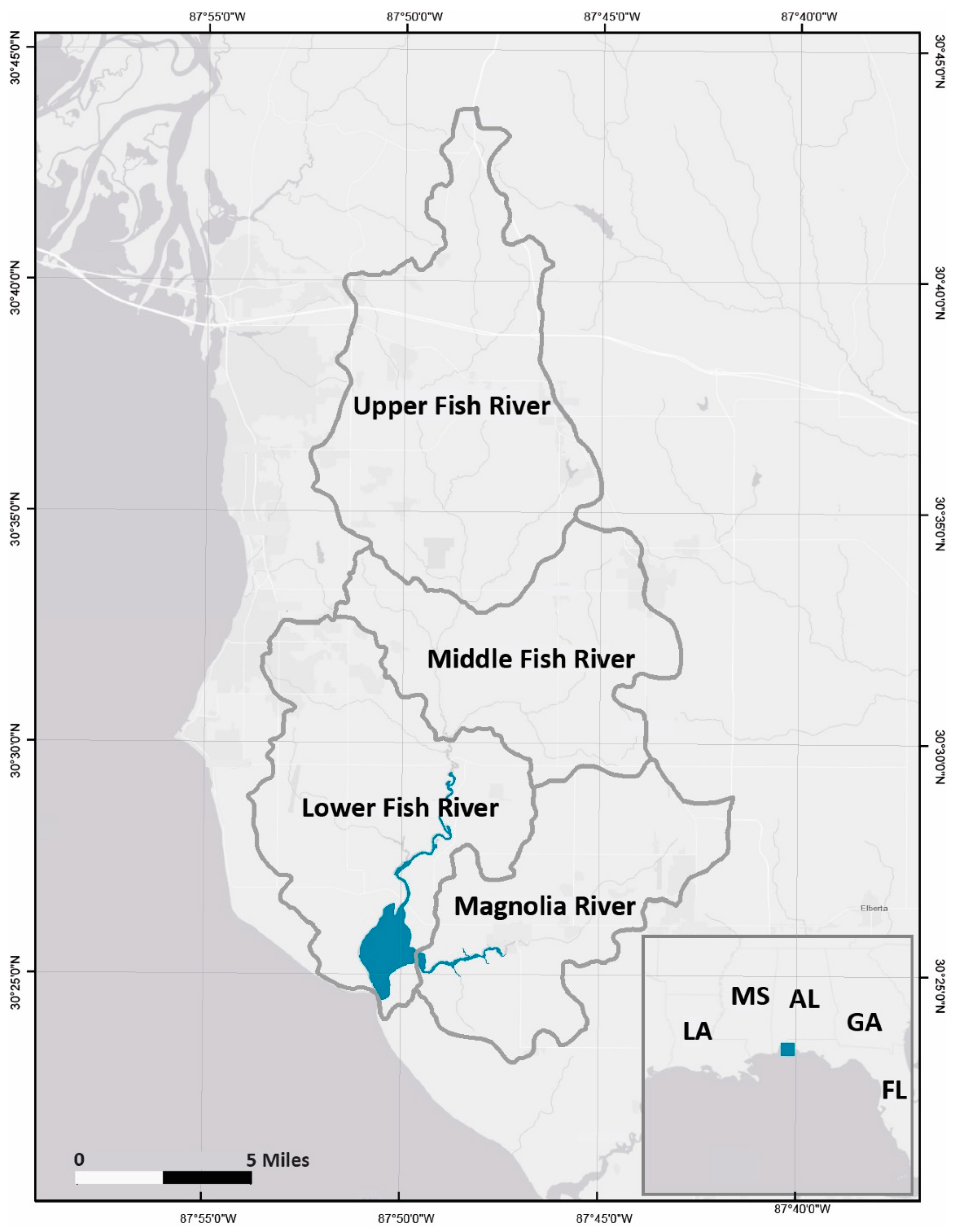
The Weeks Bay watershed is located on the eastern shore of Mobile Bay in Alabama. It is an ideal basin for the assessment of erosion potential, as it relatively small and secluded from surrounding watersheds. The watershed is limited to inputs from two major rivers (Fish and Magnolia) that both directly drain to Weeks Bay (Figure 1). The Weeks Bay watershed is a diverse natural and anthropogenically influenced landscape with natural, forested, agricultural, and developed areas that are reflective of the region’s natural resources and demographics [52]. The area is within the humid subtropical climate region, characterized by warm summers and relatively mild winters. Average annual precipitation averages about 165 cm due to winter storms (cold fronts), summer thunderstorms (including those from the sea breeze), and tropical systems. The abundant water resources in the area make for a range of very productive land uses from timber production, cash-grain crops, and forage production [53]. The Fish River provides nearly 75% of the total discharge to the bay itself and is made up of three sub-watersheds (Upper, Middle, and Lower Fish River). The Magnolia River provides the remaining discharge and consist of a single sub-watershed.
2.2. Data Collection and Processing
The process used to map soil-erosion potential was based on several geospatial variables. National data sources were used for these variables to ensure transition between different watersheds and scalability. Below, we describe the most relevant variables to be included in the model.
2.2.1. Slope
The slope for the study area was calculated using the USGS (United States Geological Survey) 30-m National Elevation Dataset (https://www.usgs.gov/3d-elevation-program; accessed on 9 October 2019). The slope calculation for each raster cell was based on the amount of descent between it and the surrounding eight cell neighborhoods using Horn’s algorithm [54]. The maximum value of descent was, thus, recorded as the cell’s slope, and could be calculated in percent or degrees. The slope raster was then normalized to 0–1.
2.2.2. Soil Erodibility
The soil erodibility (K-factor) was from the 30-m gridded USDA (United State Department of Agriculture) Soil Survey Geographic Database (https://www.nrcs.usda.gov/wps/portal/nrcs/main/soils/survey/; accessed on 10 March 2020). K-factor accounts for both the susceptibility of a cell to soil erosion based on soil texture and rate of runoff. Values less than 0.2 are considered as low erodibility, 0.2 to 0.4 as moderate, and greater than 0.4 as high, according to the National Soil Survey Handbook developed by the U.S. Department of Agriculture, Natural Resources Conservation Service (http://www.nrcs.usda.gov/wps/portal/nrcs/detail/soils/ref/?cid=nrcs142p2_054242; accessed on 1 April 2019). The values were normalized to 0.049–1.
2.2.3. Stream Density
The stream density was a 30-m raster collected from the USGS National Hydrography Dataset (https://www.usgs.gov/national-hydrography/national-hydrography-dataset; accessed on 9 October 2019). Higher instances of stream density are associated with increased erosion rates, specifically as they relate to the dissection of the landscape and land-drainage system interactions [55]. Similar data layers are used in soil-erosion analysis [56] and are also used in numerous landscape evolution models that simulate erosion and deposition [57]. The density function used for calculation utilized a neighborhood area with a specified search radius; all stream segments intersecting the area were counted and a continuous surface with the specified cell size was returned. The default search radius used in commercial GIS software is based on the minimal spatial dimension of the dataset [58]. The derived density surface was normalized by the maximum value within the Weeks Bay Watershed. The resulting data layer was a continuous index of stream density with unitless values ranging from 0.055–1.
2.2.4. Soil Brightness
The soil brightness was calculated dynamically from the tasseled cap transformation of the 30-m Land cover raster from USGS Global Land Survey Dataset (https://www.usgs.gov/landsat-missions/global-land-survey-gls; accessed on 9 October 2019). Hence, the soil brightness band of the Tasseled Cap transformation provided an index of measure for soil reflectance/exposure and not just the lack of vegetation [59]. The soil brightness data from the GLS dataset were extracted, subset to the Weeks Bay Watershed, and normalized by the maximum value. The resulting data layer was a continuous index of soil brightness with unitless values ranging from 0.018–1.
2.2.5. Precipitation
The precipitation data were collected from the 4-km 30-year normal grid of PRISM dataset (https://prism.oregonstate.edu/normals/; accessed on 15 March 2020) for rainfall variation across the basin. These data were extracted from the database for the region of interest, normalized by the maximum value, and resampled to 30 m (from 4 km). The resulting data layer was a continuous index of annual precipitation climatology with unitless values ranging from 0.96–1.
2.3. Model Description
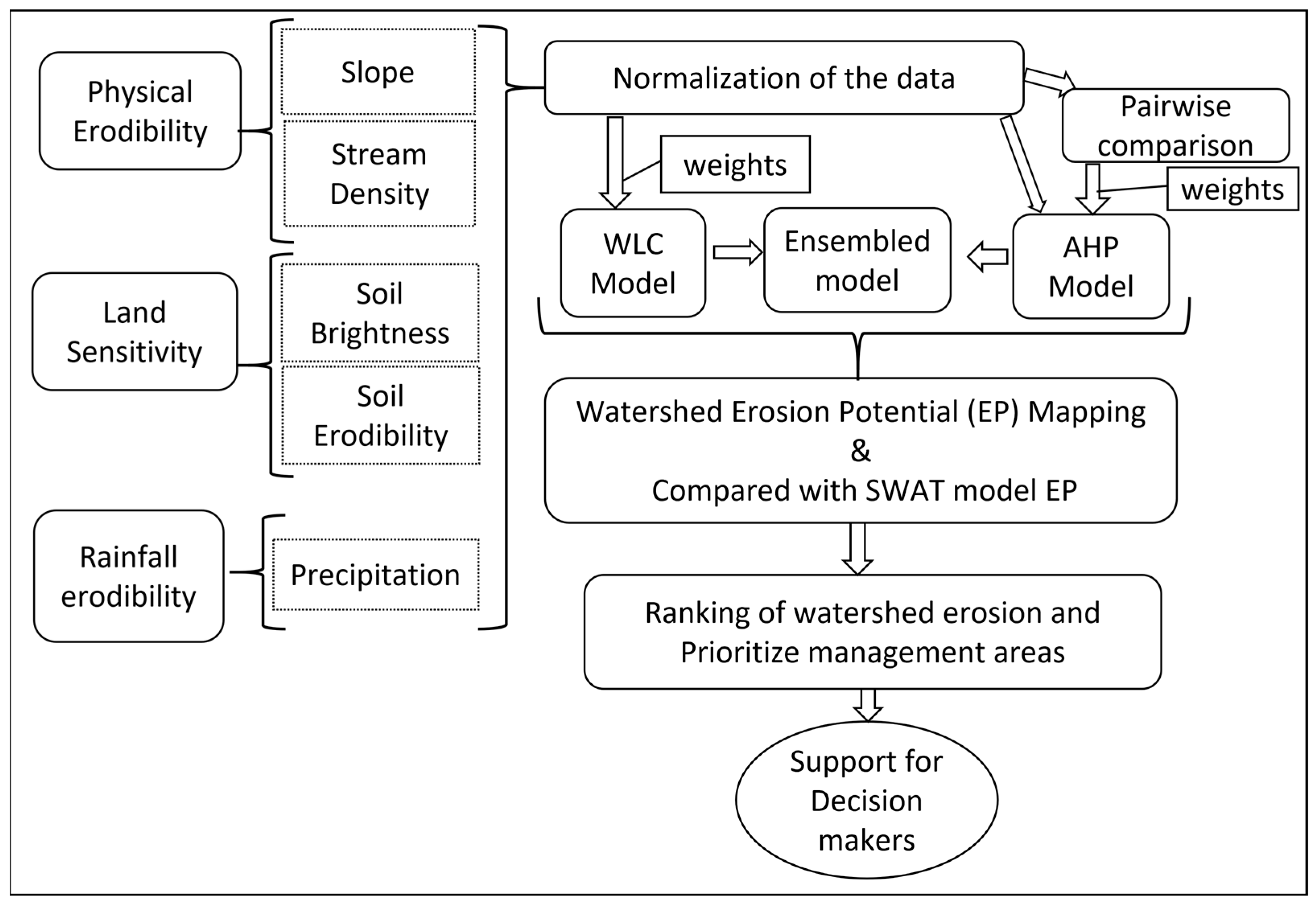
The concept of watershed erosion is summarized as the total erosion for the combination of physical erodibility, land sensitivity, and precipitation erosivity factors [20,23,41,56]. For this study area, the physical erodibility was measured by slope and stream density; land sensitivity included measures of soil K-factor and soil brightness (exposure); and rainfall erosivity was measured as average precipitation of the watershed (rainfall variation). A schematic diagram of the modeling approach for watershed erosion potential is indicated in Figure 2. The algorithm used for this WLC mapping was a standard weighted linear combination (WLC) for the summation of the five raster data layers, i.e., slope, stream density, soil brightness, soil erodibility, and precipitation [37]. The weights for the AHP model were calculated using Saaty’s method of a continuous rating scale for pairwise comparison [46]. This procedure set each data layer with a possible data range of zero to one for a common scale of assessment. Zero would be a minimal impact on erosion potential, with values of one having the greatest impact. The scale for the AHP model is shown in Table 1. Each data layer was then compared individually with the other data layers as they relate to erosion potential. Weights for each data layer were assigned based on results from the pairwise comparison matrix (Table 1). With all layers standardized and weighted, the WLC was used to apply the weights from the expert input for the assessment of erosion potential. This allowed each data layer to be multiplied by the expert-defined weight and then summed for a continuous surface of overall erosion potential. The algorithm for the WLC and AHP model is shown in the Equations (1) and (2), respectively.
where is the watershed erosion potential, is the average Precipitation, is the soil erodibility, is the slope length and steepness, is the soil brightness, and is the stream density of this region. is the standard weight for the WLC model, and , , , , and are weights expected from running the AHP model.
The erosion potential (EPEN) from the ensembled model was calculated and is mentioned in Equation (3).
where is the ensembled erosion-potential model, is the number of models, and indicates the erosion potential from each of the ith models.
2.4. Sensitivity Analysis
A basic sensitivity assessment was performed for the WLC model variables. The assessment was a simplistic one-at-a-time (OAT) procedure wherein a single variable or layer was removed and the erosion-potential analysis was processed again. The procedure followed the method used by Chen et al. [34] and Romano et al. [36].
2.5. Ranking of the Management Area
The study area was divided into 18 management areas based on the smaller streams in the watershed. The management areas were ranked or prioritized based on the average EP value for each zone. The average EP values found in the WLC, AHP, and SWAT models were compared to visualize the similarities in the zones’ priorities for management, to support improved decision making for management and prioritization of resources.
3. Results
3.1. WLC Model
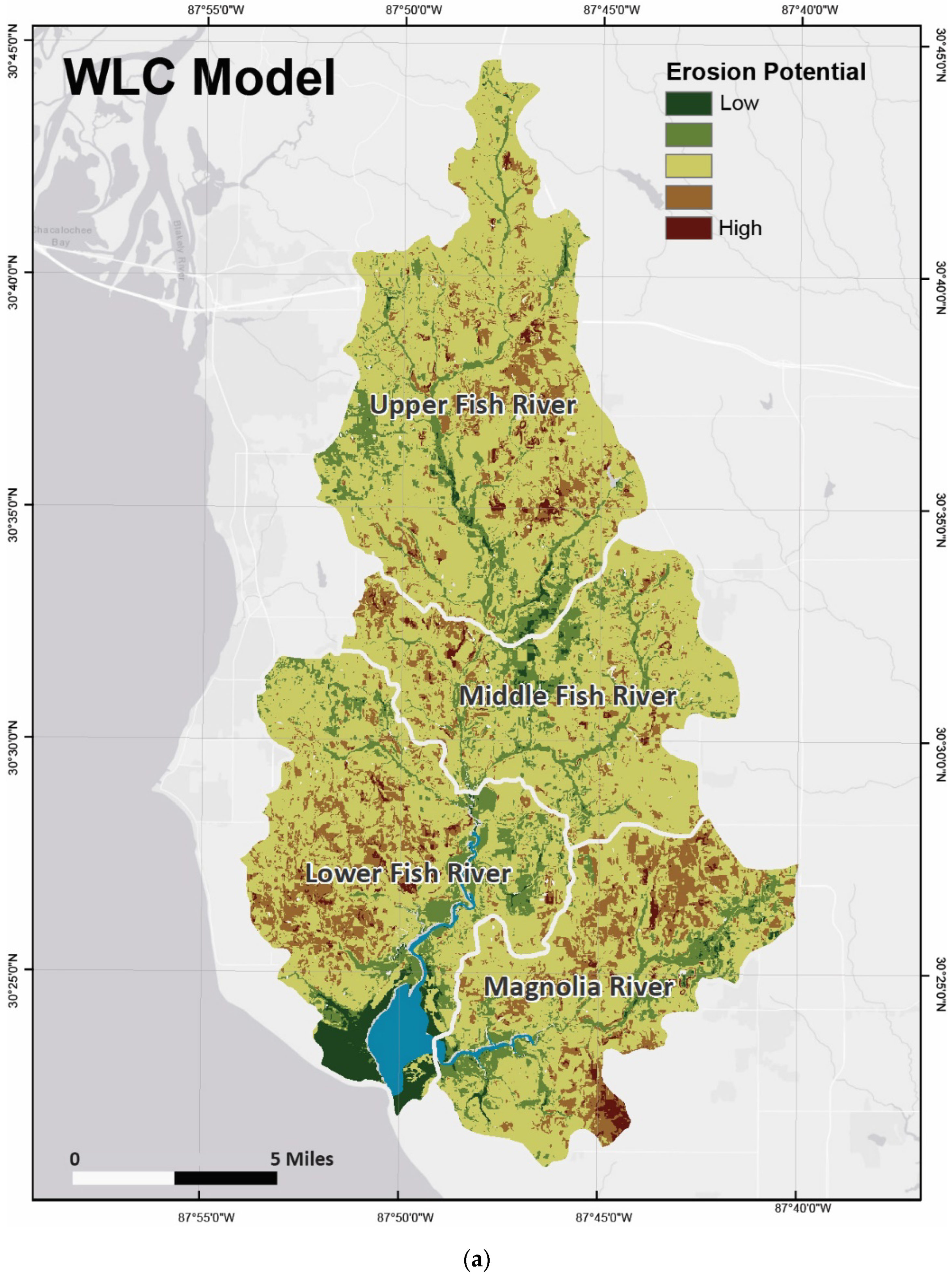
Potential watershed erosion cells were mapped with a standard weighted linear combination (WLC) to build a foundation for the qualitative assessment for watershed erosion. Criteria sensitivity was evaluated using the one-at-a-time (OAT) method to better understand the influence of the landscape layers. The WLC model was executed using the five raster data layers, weighted equally, for the initial assessment of generalized erosion potential. The output of the WLC model was a continuous surface of erosion potential based on physical erodibility, land sensitivity, and 30-year precipitation for the Weeks Bay watershed. Mean erosion potential was calculated for the entire watershed (0.527, S.D. = 0.057) and the four sub-basins within the Weeks Bay watershed. Field observations during site visits showed that the upland, head water areas of the watershed, and the areas dominated by cultivated agricultural areas are expected to have higher erosion potential. Lower erosion-potential values are expected in the densely vegetated riparian and marsh areas.
The erosion-potential data were classified based on the standard deviation spread from the mean erosion potential across the drainage basin, to better define areas based on the upper and lower ranks of erosion potential. This resulted in seven classes that were used to define the ranks for the cells, with class 1 having the lowest potential and class 7 having the highest potential. At the watershed level, 1.5% of the cells are in the upper-most erosion-potential ranks (classes 6 and 7), approximately 14% are in the moderate erosion-potential rank (class 5), and the lower erosion-potential ranks (classes 1–3) are similar in distribution to the upper ranks (classes 5–7).
Erosion potential across the four sub-basins level are varied in comparison. The two downstream basins (Magnolia and Lower Fish) have decreased proportions of cells around the mean erosion potential, and the two upstream basins (Upper and Middle Fish) have increased cell proportions around the mean erosion potential. The Magnolia River sub-basin has the largest count of cells in the upper erosion-potential ranks (classes 5–7), at 23%. The Lower Fish River sub-basin has the next highest count, with almost 17% of the sub-basin in the upper erosion-potential ranks, and the Upper and Middle Fish sub-basins have 12% or less in the upper ranks. Table 2 provides a complete description of cell counts (with upper and lower ranks) at the basin and sub-basin levels.
3.2. WLC Model Criteria Sensitivity Assessment
The sensitivity of individual criteria was accessed using the one-at-a-time (OAT) method by removing one criterion from the WLC model and recalculating erosion potential. This resulted in five additional WLC model outputs of erosion potential produced by equally weighting four of the five criteria; the detailed results are mentioned in Table 3. The five additional OAT WLC models were compared to the initial WLC model to understand the influence of each variable in the WLC. The OAT WLC models all had moderate- to-strong correlations with the initial WLC model.
The model without the precipitation variable had the strongest correlation (R = 1.00), followed by the model run without slope input (R = 0.94). The runs without stream density and soil brightness were moderately correlated, R = 0.88. The run with the weakest correlation was the one without K-factor, R = 0.79. The correlation results showed that the WLC model was most sensitive to the K-factor variable, moderately sensitive to the variables of stream density and soil brightness, and least sensitive to the precipitation and slope variables.
3.3. AHP Model
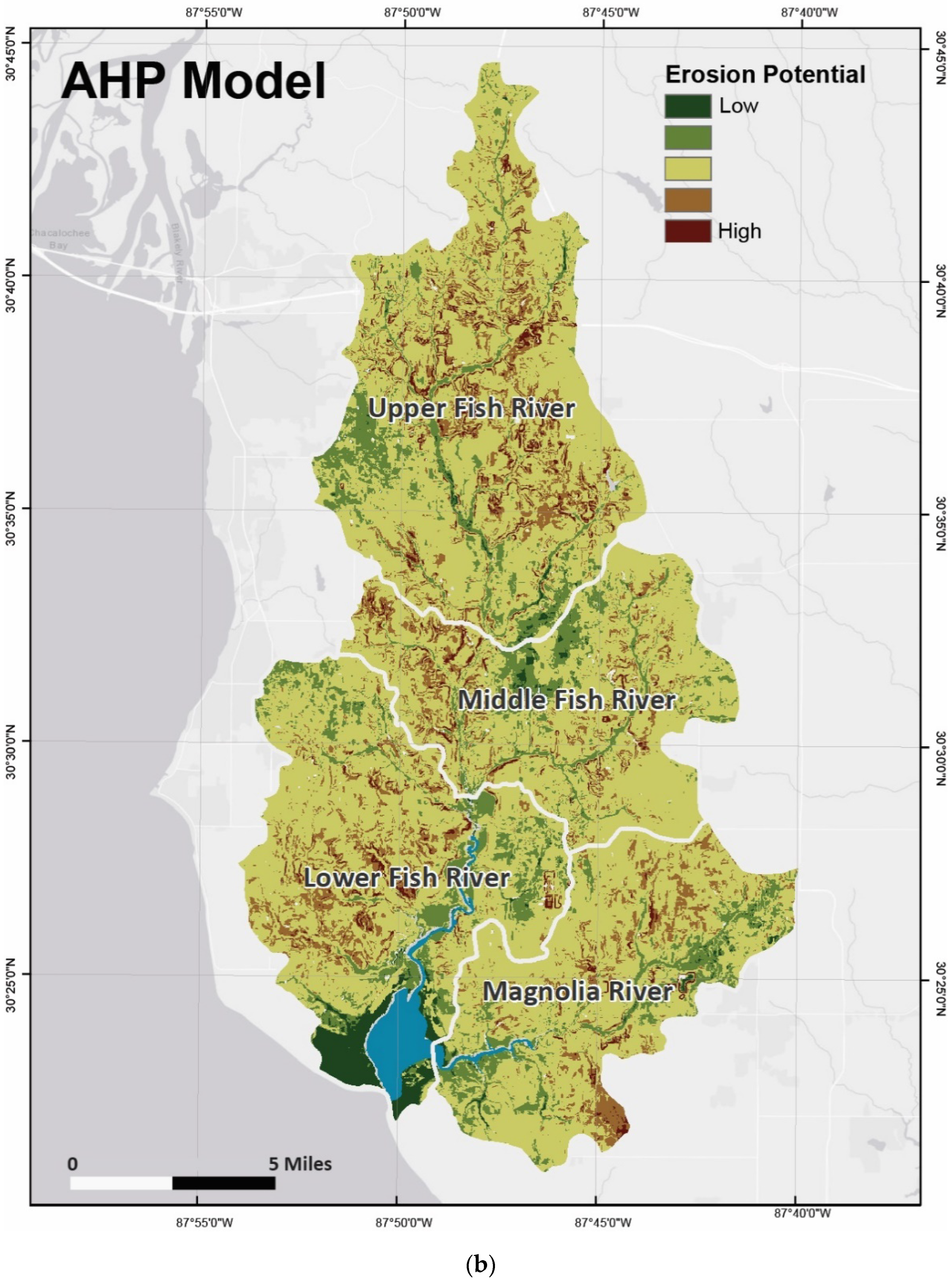
This Analytical Hierarchy Process (AHP) model was executed on the five raster data layers utilized in the WLC model. The AHP experts input defined weights for each of the five layers with the pairwise comparison. The weight assignments for each of layers were based on scores from the experts’ qualitative ranking of factors. The most weight was given to terrain slope at 33.8% with lesser weights given to geomorphology, land cover, and soil erodibility (~15.0% for each). The 30-year precipitation was effectively left unchanged at 20.5%. The AHP mean erosion potential for the entire watershed (0.472, S.D. = 0.051) decreased as compared to the WLC erosion potential. The range of the AHP erosion potential increased slightly from that of the WLC and was strongly correlated, with a Pearson’s R value of 0.923.
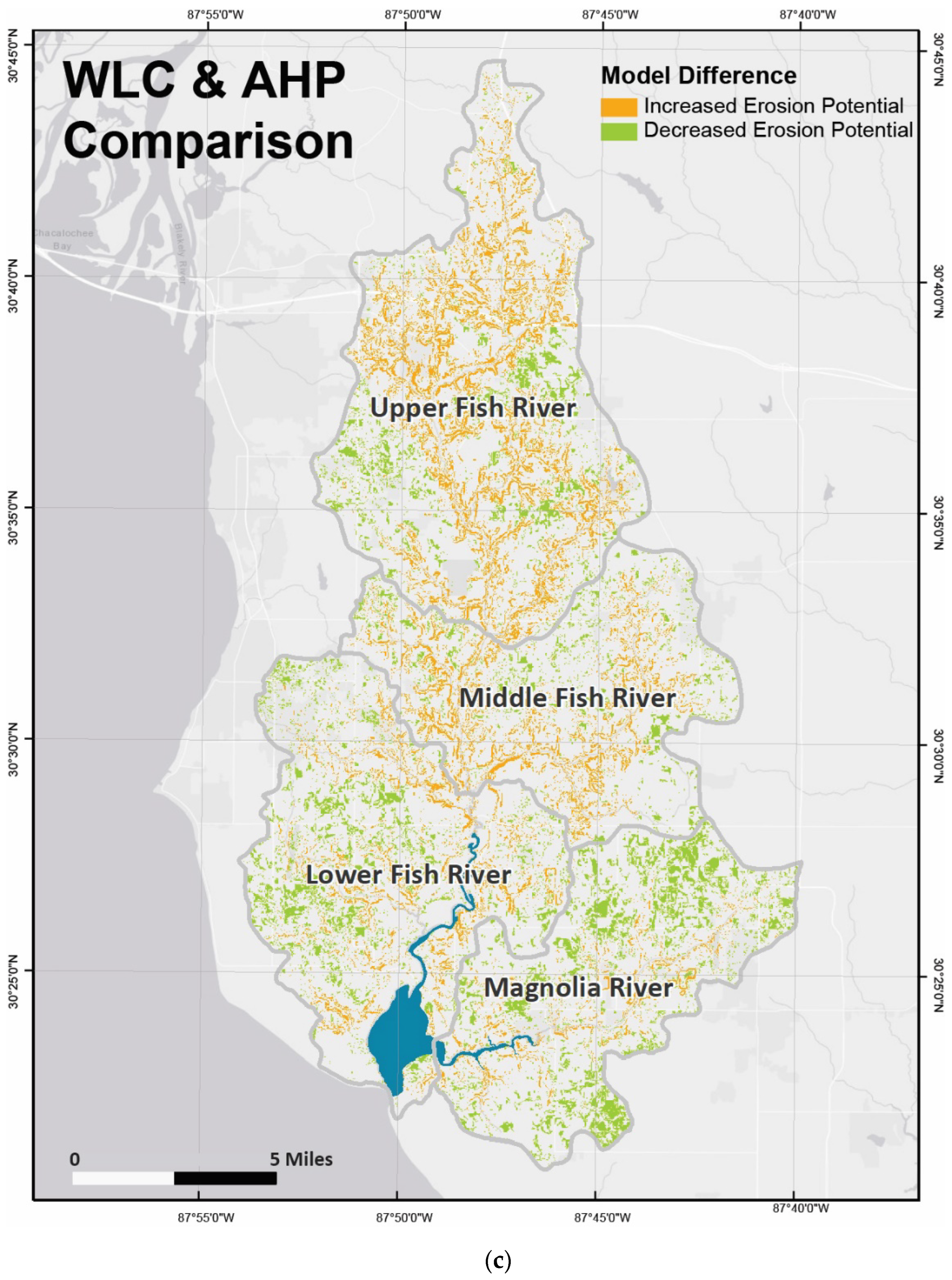
The AHP erosion-potential data were classified into seven classes based on a standard deviation spread (Figure 3b) of just the WLC erosion-potential data (Figure 3a). At the watershed level, 2.7% of the cells are in the upper-most erosion-potential ranks (classes 6 and 7) and approximately 12% are in the moderate erosion-potential rank (class 5). The lower erosion-potential ranks (classes 1 and 2) are similar to the upper ranks with 2.27% of the cells. The AHP model produces slightly more cells in the lower ranks than the upper ranks of erosion potential (Table 4). The spatial differences between the AHP model and the WLC model erosion-potential class changes are seen in Figure 3c, highlighting the areas where the AHP increased or decreased erosion potential from the WLC model.
The AHP weights were altered in one-percent increments to identify outliers with AHP model runs. An example of weight alteration in the AHP model for 41 iterations for a single layer is displayed in Appendix A, Table A1. The percentage of outliers at each map (or grid) cell was calculated to look at variations spatially. A threshold of 25% was used to define areas with minimal alignment between AHP runs. About 37.5% of the mapped watershed cells were producing inconsistent or varying erosion-potential results. About 62.5% of the mapped watershed cells were in alignment with 75% of the model runs, with no outliers. This area of the watershed is where the AHP model runs were in alignment for the upper and lower ranks of erosion potential. Erosion cell counts in this area for the moderate and upper ranks (classes 5, 6, and 7) decreased proportionally. The proportional decrease shows that the higher instances of outliers are not clumped within the lower or upper ranks of erosion potential. This provides the definition of a focus area (an analysis mask) for increased erosion potential in the Weeks Bay watershed (Figure 4). This analysis mask serves as spatial filter for mapped erosion-potential cells for improved agreement in the modeled outputs.
3.4. WLC and AHP Model Comparison
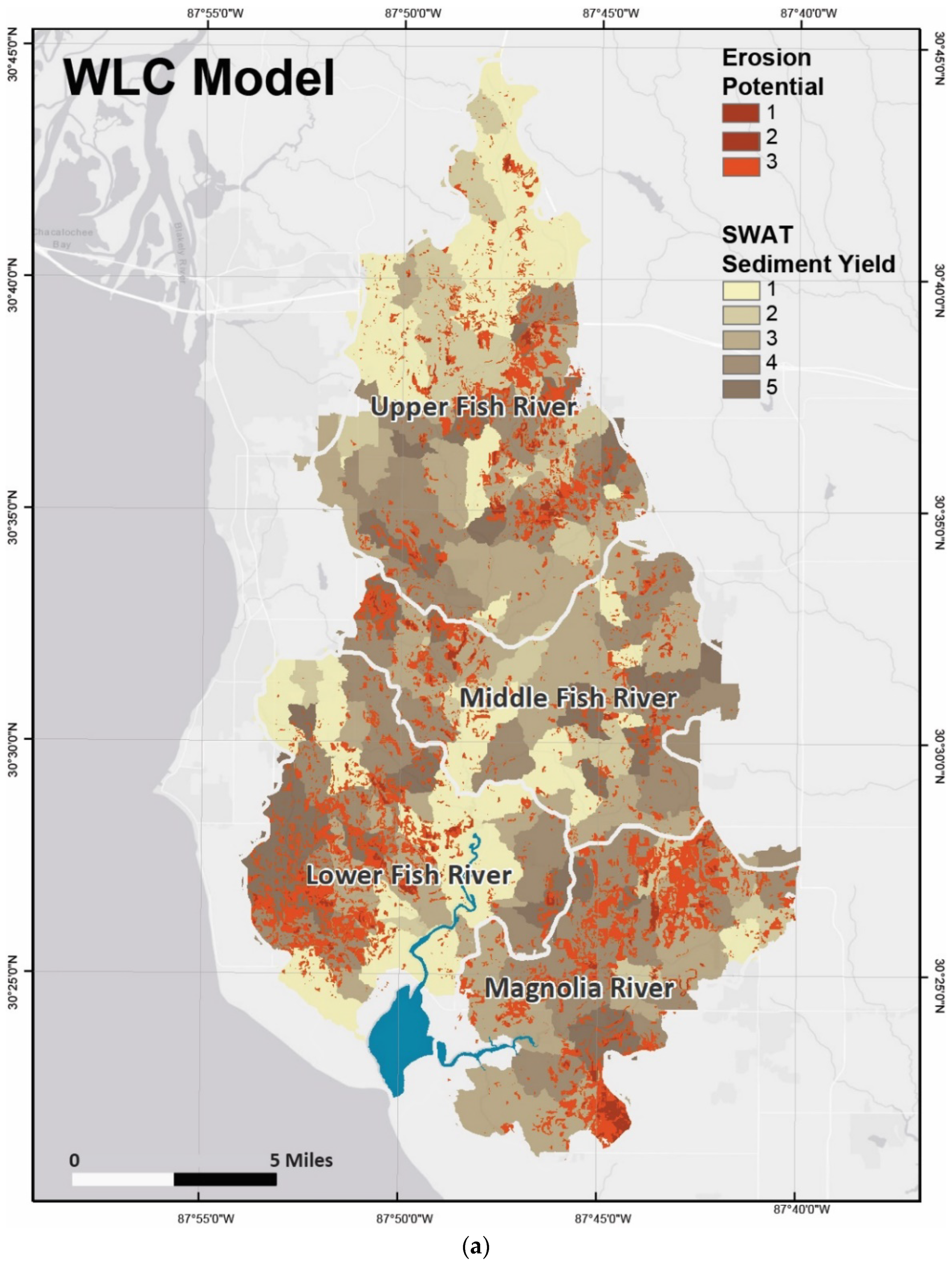
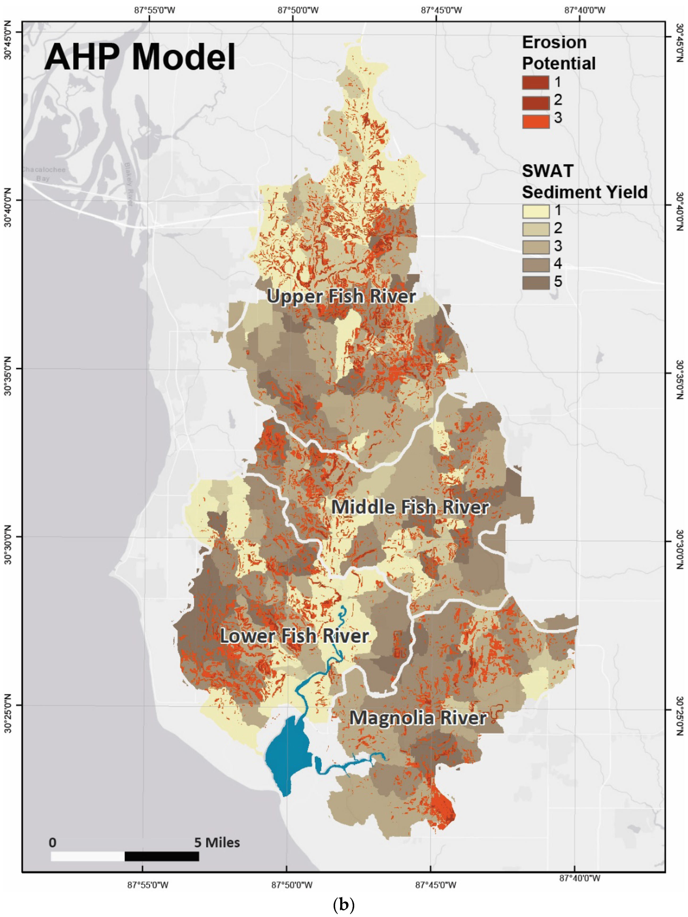
Comparisons between the WLC and AHP models were expanded to include an evaluation of the outputs with a SWAT model for the Weeks Bay Watershed. This comparison went beyond the mapped potential erosion cells to evaluate the outputs for watershed management scenarios. The comparison took the classified erosion cells for the WLC and AHP models and mapped them with the sediment-yield data for 237 sub-watersheds from the SWAT model output. The WLC and AHP data were similar, with an apparent alignment in the southwestern and northeastern areas of the watershed, with the higher ranks of mapped erosion potential aligned with the SWAT sediment yield (Figure 5). Additionally, the AHP data highlighted hillslope areas in the headland areas of the watershed due to the experts’ emphasis on topography.
3.5. Management-Priority Area Ranking
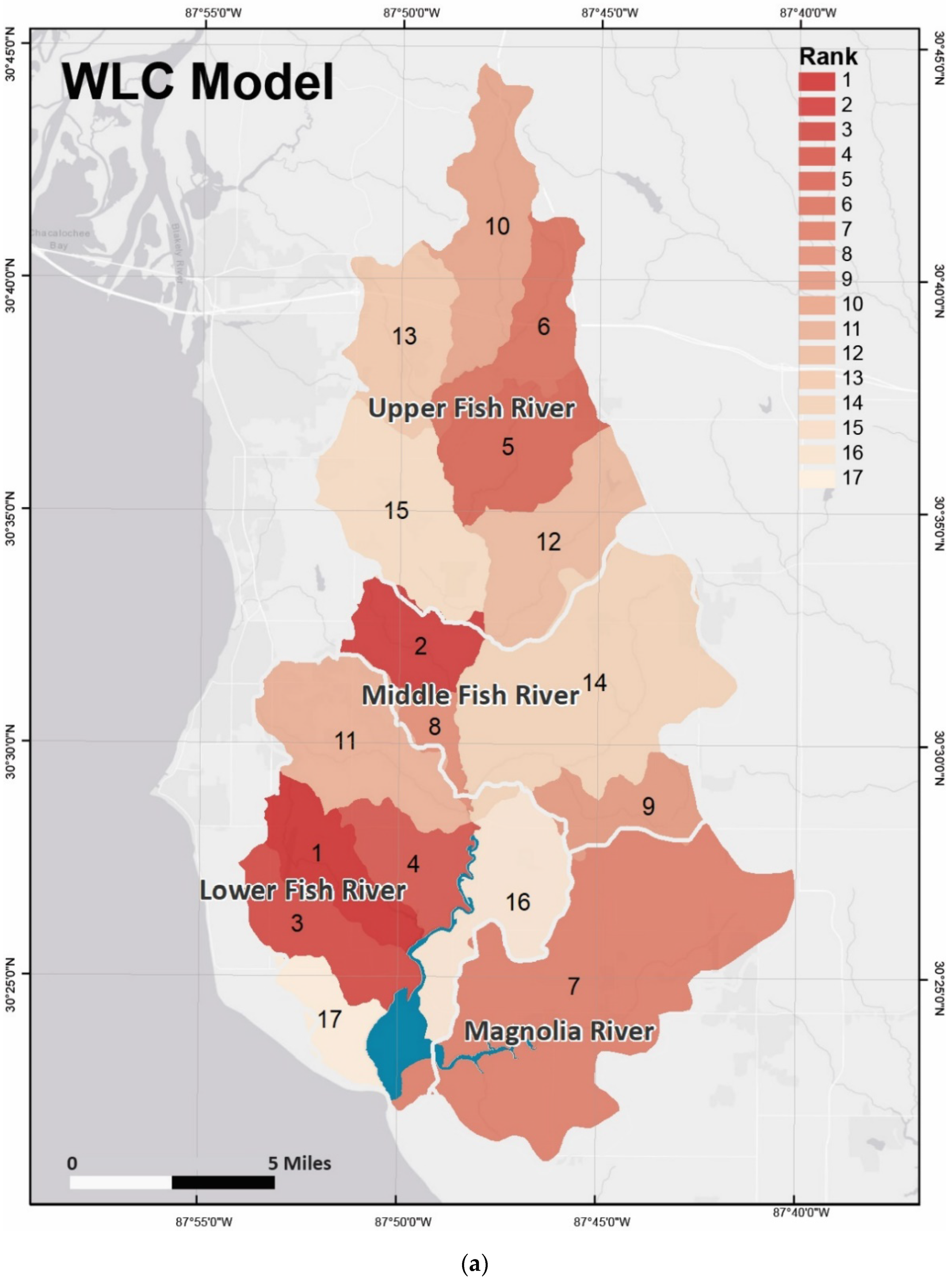
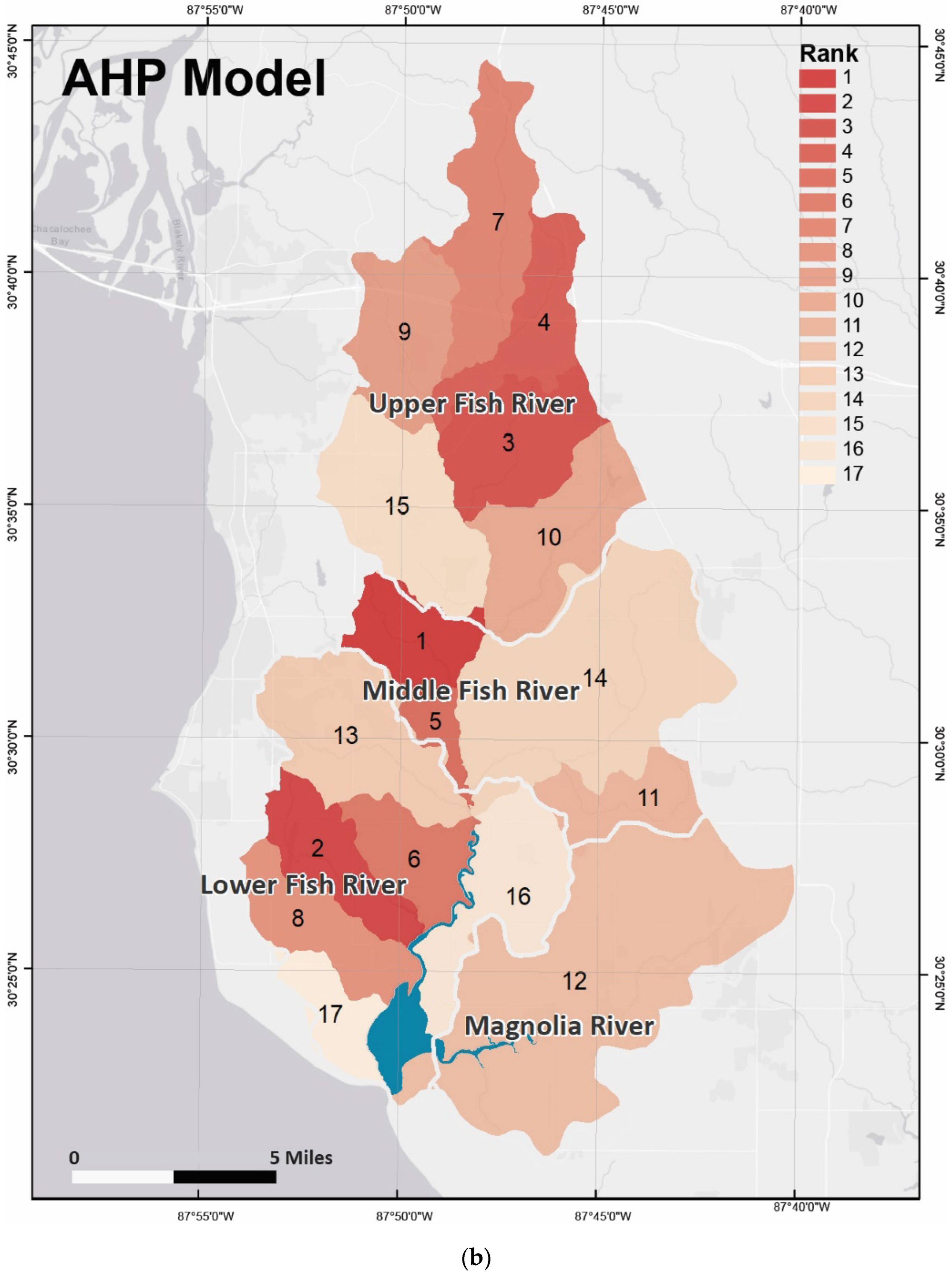
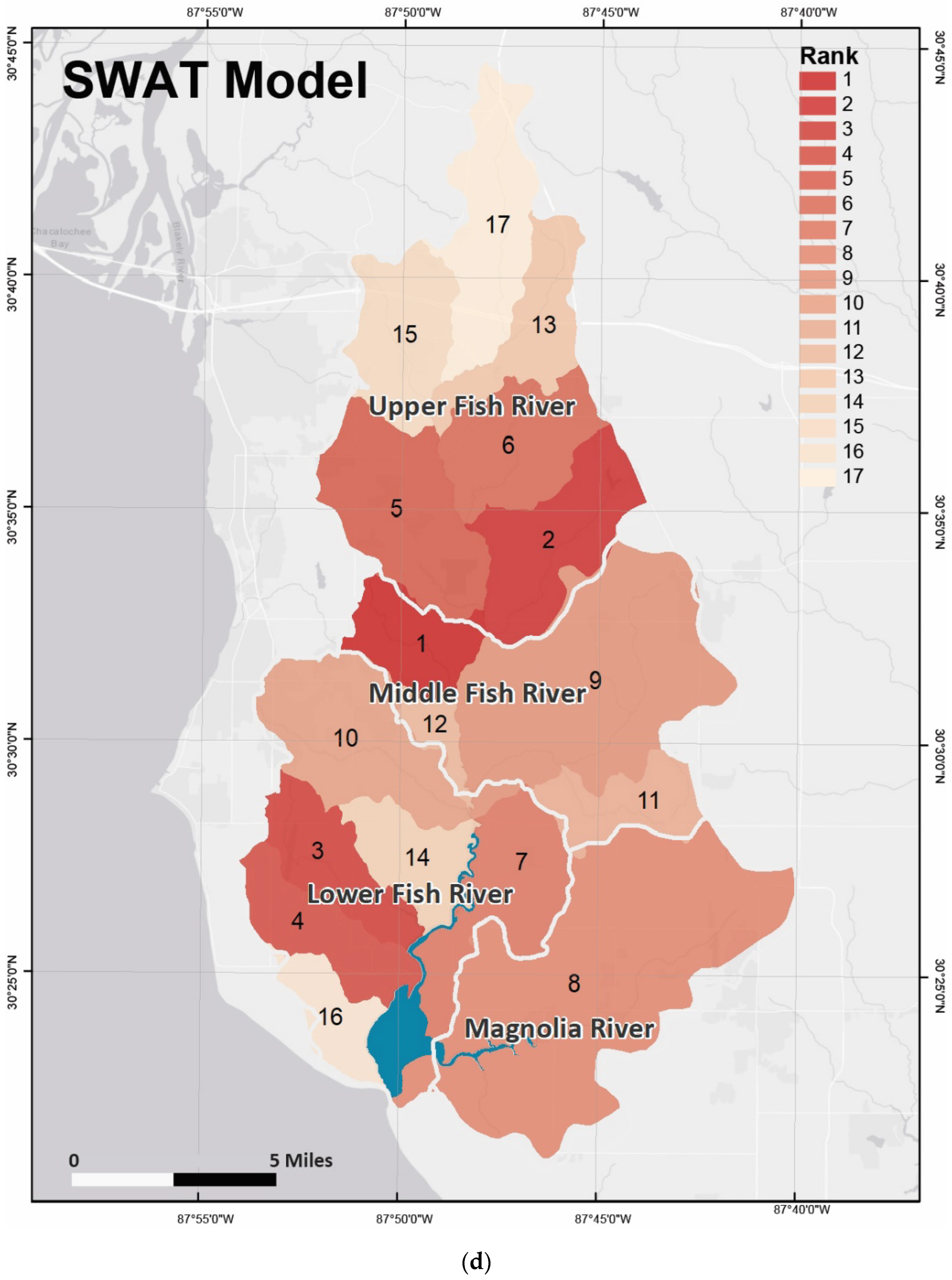
The final comparison was an aggregate of the mapped erosion-potential cells from the WLC, AHP, and ensemble model runs and the SWAT model sediment-yield data to the management areas of the Weeks Bay watershed (Figure 6). The average erosion-potential values and the SWAT sediment-yield data were summarized for each of the management areas for ranked prioritization. Observational trends in the summarized data exhibited spatial alignment in the WLC and AHP upper erosion-potential ranks with higher SWAT sediment-yield data for the watershed management areas. Both the qualitative AHP model and the numerical SWAT model agreed in mapping the management area ranked with the highest erosion. Figure 6 shows the management area rankings for the WLC, AHP, and SWAT models with the ranking of each area based on calculated erosion or sediment yield for the respective model output. The WLC, AHP, and SWAT ranks for the higher ranks of erosion aligned approximately 70% of the time.
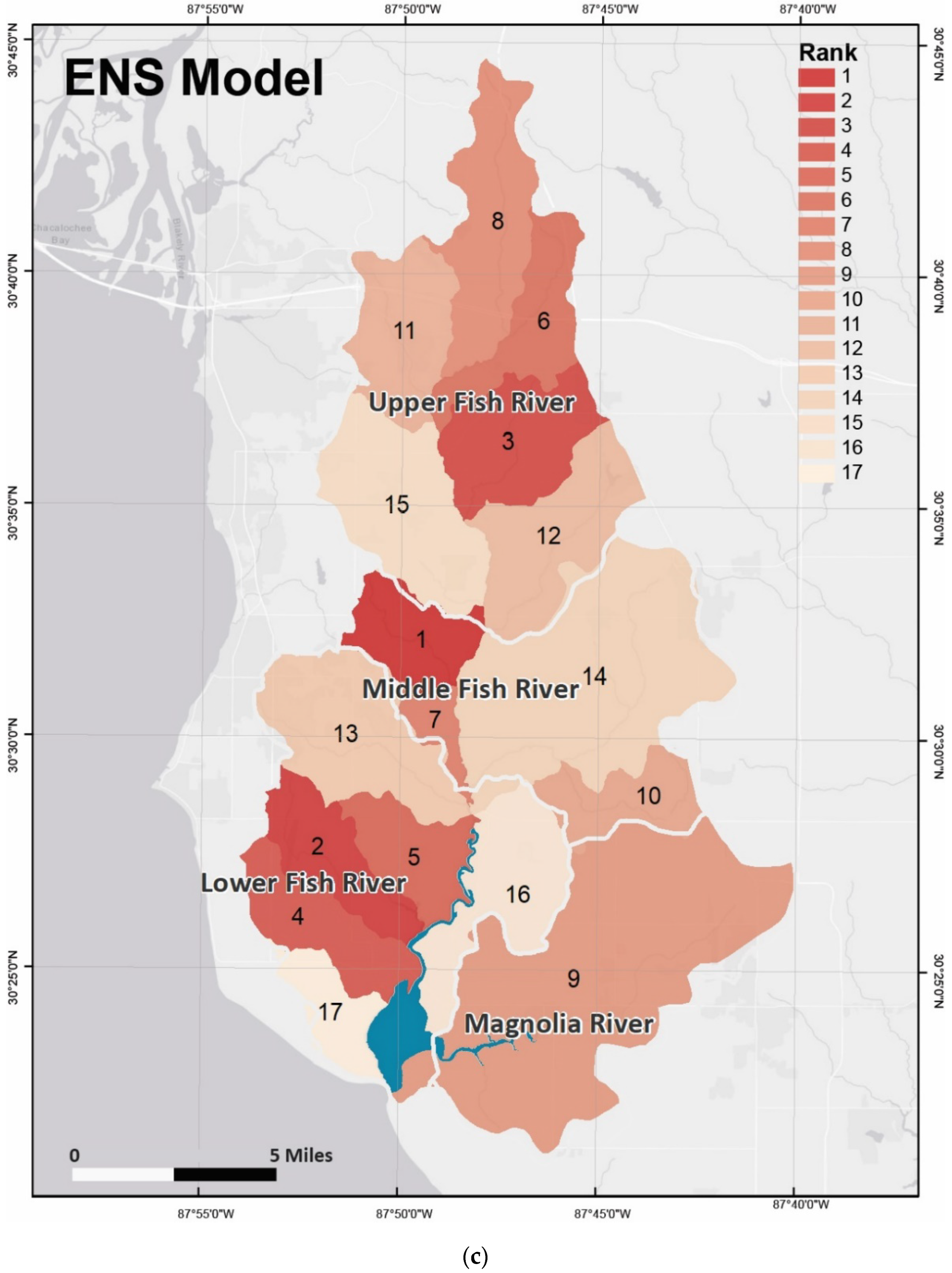
Similarly, the mapped erosion potential from the ensemble model was averaged and summarized for the management areas, and similar rankings were found to that of the SWAT model. Three of the four management areas—Pensacola Branch, Waterhole Branch, and Turkey Branch—aligned with areas ranked by the SWAT model for high sediment yield. In the lower ranks, alignment was found with the Weeks Branch and Weeks Bay management areas (Table 5). Overall, the ensembled model produced similar results to that of the WLC and AHP models, with agreement in mapped erosion potential in areas of higher ranks.
4. Discussion
The erosion potential for a watershed along the northern Gulf of Mexico was mapped qualitatively using layers representative of physical erodibility, land sensitivity, and 30-year precipitation for the Weeks Bay watershed. The criteria used to define these layers were based on regional availability and input from watershed managers and stakeholders on erosional trends in this area. The approach used a WLC model and was set up with criteria similar to numerical models such as RUSLE [19]. Other approaches to soil-erosion mapping include empirical, conceptual, physically based, and hybrid models [60]. Some hydrodynamic numerical models, i.e., 1-D (one-dimensional) and 2-D hydrodynamic models showed better efficiency in urban-flood-risk mapping [61]. Compared to the conceptual models, i.e., the Hydrologic Simulation Program (HSPF) and SWAT [60], this study proposed a WLC model which is also applicable to larger areas with less complexity. Additionally, the AHP model in the study area considered the factors’ importance in terms of being responsible for regional watershed erosion. However, this study did not show any physically based model, which could be a future demand for better estimation of erosion risk at a large scale. In addition, factors such as surface hydrology, slope aspect, and storm events could be used in 2-D physically based simulation models such as GSSHA (Grided Surface/Subsurface Hydrologic Analysis), DWSM (Dynamic Watershed Simulation Models), etc.
In this study, the northern headland and the southern agricultural regions of the watershed had the highest erosion potential, as expected [1,28]. Overall erosion potential in the Weeks Bay watershed tends to be lower in densely vegetated riparian and marsh areas. Many of these areas, especially in the southern area near the bay, are part of the Weeks Bay National Estuarine Research Reserve. Areas in the watershed with higher erosion potential are more associated with transitional-type lands that appear to be more agricultural or dynamic in terms of land practices. The southeast region of the watershed reflects this, as it is an area dominated by agricultural practices such as cultivated crops and turf-grass farms.
Land sensitivity accessed by soil erodibility (as defined by the soil K-factor and soil exposure or brightness) was the criterion that had the most influence on mapped erosion potential with the WLC model. The K-factor is used in USLE and RUSLE applications that represents soil texture and composition [19,20,24], and was the most influential of the layers. Soil brightness is indicative of disruptive land uses and increases in erosion potential from this variable are apparent in agriculture-dominated areas of the watershed. The physical erodibility (topographic) criteria for slope and stream density moderately influenced the WLC-modeled erosion potential. These areas of increased potential are indicative of higher concentrations of stream reaches, with more surface interaction with runoff waters and lower soil infiltration rates [55], and proximity to active stream and river channels.
The assessment was enhanced with expert input through the AHP model, allowing experts to rank the criteria. The ranking of criteria quantified the weights based on their relative importance in the study area. The physical erodibility criterion of slope was identified as the most important by the experts. In this, the AHP model differs from the traditional soil-erosion models, with the experts’ minimal emphasis on land cover or land sensitivity [19,21]. This difference is also concerning due to the increased erosion rates due to development in the watersheds in this region of the Gulf of Mexico [52]. The AHP model proved to be beneficial in mapping areas of increased erosion potential, as defined by the upper ranks in the classified data. These shifts of the mapped erosion cells from the WLC model align with similar approaches using MCDA techniques [42,55]. The AHP model is not a typical numerical model and can be better-suited to qualitative geospatial assessment for mapping erosion potential with MCDA.
The variations in the AHP weights are normally used to identify shifts (increasing and decreasing) in the mapped erosion-potential cells. Data outliers were used for the identification of areas of model alignment for the high ranks of erosion potential. This approach allowed for an analysis (management) mask to be generated for these areas that were consistently high, irrespective of the variation in criteria weights. The areas identified were generally associated with higher slopes, which were associated with stream and channel networks. The outlier analysis was successful in helping to identify management areas; however, a suitable model approach would allow for a quantification shift between ranks of erosion potential [34,39,45].
The WLC and AHP erosion-potential models were run as an ensemble to improve the reliability of the output. The outputs (from models) were compared with the SWAT sediment yield; the comparisons were used to help identify if there were any visual alignments or trends between the qualitative and quantitative outputs. The comparisons were very similar, with the primary difference being the focus of higher erosion-potential values in the WLC and AHP models. The alignment of the data was most apparent in areas of transition with expanding development and agricultural land practices. The AHP model, however, produced some areas that were more focused on topographic features because of the experts’ input placing more emphasis on physical erodibility (slope and other terrain measures). This was most apparent in the headland area of the watershed where the landscape has more dissection. The comparison of prioritization and ranking of the mapped erosion-potential cells for Weeks Bay Watershed management areas displayed alignment for select areas of higher erosion potential.
These management areas include the Pensacola Branch, Waterhole Branch, and Turkey Branch basins of the Weeks Bay Watershed. Each of these management areas have experienced increased erosion due to expanding land development associated with the surrounding communities. The management areas with the lowest ranks were also in agreement. This, coupled with the alignment in the upper ranks, indicates a generalized agreement between the qualitative and quantitative assessments for the prioritization of management areas. The approach has limitations in management areas that would be considered to be of intermediate concern with regard to erosion. This is, in part, due to various reasons, including the added emphasis by the experts on terrain characteristics and temporal generalizations in layers used in the WLC/AHP models and the SWAT model.
However, these areas of upper and lower erosion ranks are indicative of the agreement between the qualitative and quantitative modeling approaches, supporting the use of MCDA for management decisions and improved applications for watershed managers.
5. Conclusions
The watersheds that drain areas along the northern Gulf of Mexico have dynamic landscapes that experience erosion and contribute volumes of sediment to the associated estuaries. These watersheds and their estuaries are important for both their services and the resources they provide. To maintain the function and value of these services and resources, these areas require proper management in terms of soil-loss and erosion. Those involved in the management of these watersheds and the associated resources need to have information that is both accurate and timely. This study took an approach that focused on a qualitative assessment with GIS and MCDA for mapping erosion potential, to facilitate the prioritization of watershed management areas for improved management decisions. This aim of this approach was to provide watershed managers with a process to quickly map erosion potential and prioritize areas for management. This will allow for better and more efficient allocation of resources to be utilized in watershed management for areas such as the Weeks Bay watershed.
Field measurements and numerical models are critical to accurately measure and estimate sediment yield and erosion, as they provide quantitative information to facilitate management plans and decisions. Qualitative assessments can produce similar results and help in the management process. Qualitative assessments do not provide numerical sediment-yield information, but often provide more rapid assessments with a more simplistic approach and execution. The design of these assessments needs to be similar to numerical modeling approaches, using similar criteria and inputs. Their design can also allow for expert input for situation-specific applications due to their understanding of the processes and issues unique to the watershed of interest. A WLC model and an AHP model were used to map erosion potential based on terrain slope, geomorphology, land cover, soil erodibility, and long-term precipitation trends.
The WLC and AHP models developed for this study mapped erosion potential to cells as defined by the input layers for the Weeks Bay watershed. The mapped erosion potential aligned with the erosion trends described in the Weeks Bay Watershed Management Plan, with increased erosion occurring in areas associated with agricultural practices and expanding areas of urban and suburban development. The MCDA with the AHP model mapped areas that are most susceptible to erosion, as evidenced by the shifts of cells in the upper ranks. This, coupled with the analysis mask generated by the criteria weighting variations, identified areas of alignment or commonality in erosion potential in the Weeks Bay watershed. These areas, in both the WLC and AHP models, were in agreement with the SWAT sediment-yield data from the Weeks Bay Watershed Management Plan. The qualitative approach was effective in prioritizing management areas in the Weeks Bay watershed and offers a simplified approach to mapping erosion potential. This simplified approach provides watershed managers with the means to define and prioritize management actions. This does not replace the need for numerical modeling for quantitative soil-erosion metrics; it does, however, provide management alternatives when needed. There are numerous pathways for future research for this work. Refinement and adaptation of the qualitative approach will continue to improve reliability as compared with numerical model outputs such as sediment yield. This will involve more interactions with modelers and watershed managers (and stakeholders). Scaling the approach to a regional level in future efforts could be beneficial in prioritizing modeling needs and guidance in watershed management plan needs. This, coupled with more development of geospatial tools, would help to transition these types of approaches to a more operational environment, allowing for enhanced planning and management-scenario development.
Author Contributions
Conceptualization, J.H.C., S.A.S., J.C.R.III; Data curation, J.H.C.; Formal analysis, J.H.C., S.A.S., J.C.R.III; Funding acquisition, J.H.C.; Investigation, J.H.C.; Methodology, J.H.C., S.A.S.; Supervision, J.C.R.III; Validation, J.H.C., S.A.S.; Visualization, J.H.C., S.A.S.; Writing—original draft, J.H.C., S.A.S.; Writing—review & editing, J.H.C., S.A.S., J.C.R.III. All authors have read and agreed to the published version of the manuscript.
Funding
This paper was supported through the Geospatial Education and Outreach Project funded by the National Oceanic and Atmospheric Administration Regional Geospatial Modeling Grant, award # NA19NOS4730297.
Conflicts of Interest
The authors declare no conflict of interest. The funders had no role in the design of the study; in the collection, analyses, or interpretation of data; in the writing of the manuscript; or in the decision to publish the results.
Appendix A

Table A1.
Criteria weight variation example for 41 iterations in each data layer in the AHP model.
| No. of Iterations | Slope | Stream Density | K-Factor | Soil Brightness | Precipitation |
|---|---|---|---|---|---|
| −20 | 0.270 | 0.184 | 0.166 | 0.158 | 0.222 |
| −19 | 0.274 | 0.183 | 0.165 | 0.157 | 0.221 |
| −18 | 0.277 | 0.182 | 0.164 | 0.156 | 0.220 |
| −17 | 0.281 | 0.181 | 0.164 | 0.155 | 0.219 |
| −16 | 0.284 | 0.180 | 0.163 | 0.154 | 0.219 |
| −15 | 0.287 | 0.180 | 0.162 | 0.154 | 0.218 |
| −14 | 0.291 | 0.179 | 0.161 | 0.153 | 0.217 |
| −13 | 0.294 | 0.178 | 0.160 | 0.152 | 0.216 |
| −12 | 0.297 | 0.177 | 0.159 | 0.151 | 0.215 |
| −11 | 0.301 | 0.176 | 0.158 | 0.150 | 0.214 |
| −10 | 0.304 | 0.175 | 0.158 | 0.149 | 0.213 |
| −9 | 0.308 | 0.175 | 0.157 | 0.148 | 0.213 |
| −8 | 0.311 | 0.174 | 0.156 | 0.148 | 0.212 |
| −7 | 0.314 | 0.173 | 0.155 | 0.147 | 0.211 |
| −6 | 0.318 | 0.172 | 0.154 | 0.146 | 0.210 |
| −5 | 0.321 | 0.171 | 0.153 | 0.145 | 0.209 |
| −4 | 0.324 | 0.170 | 0.153 | 0.144 | 0.208 |
| −3 | 0.328 | 0.169 | 0.152 | 0.143 | 0.208 |
| −2 | 0.331 | 0.169 | 0.151 | 0.143 | 0.207 |
| −1 | 0.335 | 0.168 | 0.150 | 0.142 | 0.206 |
| 0 | 0.338 | 0.167 | 0.149 | 0.141 | 0.205 |
| 1 | 0.341 | 0.166 | 0.148 | 0.140 | 0.204 |
| 2 | 0.345 | 0.165 | 0.147 | 0.139 | 0.203 |
| 3 | 0.348 | 0.164 | 0.147 | 0.138 | 0.202 |
| 4 | 0.352 | 0.164 | 0.146 | 0.137 | 0.202 |
| 5 | 0.355 | 0.163 | 0.145 | 0.137 | 0.201 |
| 6 | 0.358 | 0.162 | 0.144 | 0.136 | 0.200 |
| 7 | 0.362 | 0.161 | 0.143 | 0.135 | 0.199 |
| 8 | 0.365 | 0.160 | 0.142 | 0.134 | 0.198 |
| 9 | 0.368 | 0.159 | 0.142 | 0.133 | 0.197 |
| 10 | 0.372 | 0.158 | 0.141 | 0.132 | 0.197 |
| 11 | 0.375 | 0.158 | 0.140 | 0.132 | 0.196 |
| 12 | 0.379 | 0.157 | 0.139 | 0.131 | 0.195 |
| 13 | 0.382 | 0.156 | 0.138 | 0.130 | 0.194 |
| 14 | 0.385 | 0.155 | 0.137 | 0.129 | 0.193 |
| 15 | 0.389 | 0.154 | 0.137 | 0.128 | 0.192 |
| 16 | 0.392 | 0.153 | 0.136 | 0.127 | 0.191 |
| 17 | 0.395 | 0.153 | 0.135 | 0.127 | 0.191 |
| 18 | 0.399 | 0.152 | 0.134 | 0.126 | 0.190 |
| 19 | 0.402 | 0.151 | 0.133 | 0.125 | 0.189 |
| 20 | 0.406 | 0.150 | 0.132 | 0.124 | 0.188 |
References
- Basnyat, P.; Teeter, L.D.; Flynn, K.M.; Lockaby, B.G. Relationships between landscape characteristics and nonpoint source pollution inputs to coastal estuaries. Environ. Manag. 1999, 23, 539–549. [Google Scholar] [CrossRef] [PubMed]
- Wang, Y.; Yu, X.; He, K.; Li, Q.; Zhang, Y.; Song, S. Dynamic simulation of land use change in Jihe watershed based on CA-Markov model. Trans. Chin. Soc. Agric. Eng. 2011, 27, 330–336. [Google Scholar]
- Zhang, X.; Zhou, L.; Zheng, Q. Prediction of landscape pattern changes in a coastal river basin in south-eastern China. Int. J. Environ. Sci. Technol. 2019, 16, 6367–6376. [Google Scholar] [CrossRef]
- Neary, D.G.; Swank, W.T.; Riekerk, H. An overview of nonpoint source pollution in the Southern United States. In Proceedings of the symposium The Forested Wetlands of the Southern United States, Orlando, FL, USA, 12–14 July 1988; pp. 1–7. [Google Scholar]
- Wang, S.; Zhang, Z.; Wang, X. Land use change and prediction in the Baimahe Basin using GIS and CA-Markov model. In IOP Conference Series: Earth and Environmental Science; IOP Publishing: Bristol, UK, 2014; Volume 17, p. 012074. [Google Scholar]
- Ward, N.D.; Bianchi, T.S.; Medeiros, P.M.; Seidel, M.; Richey, J.E.; Keil, R.G.; Sawakuchi, H.O. Where carbon goes when water flows: Carbon cycling across the aquatic continuum. Front. Mar. Sci. 2017, 4, 7. [Google Scholar] [CrossRef] [Green Version]
- Jones, B.G.; Killian, H.E.; Chenhall, B.E.; Sloss, C.R. Anthropogenic effects in a coastal lagoon: Geochemical characterization of Burrill Lake, NSW, Australia. J. Coast. Res. 2003, 19, 621–632. [Google Scholar]
- Reusser, L.; Bierman, P.; Rood, D. Quantifying human impacts on rates of erosion and sediment transport at a landscape scale. Geology 2015, 43, 171–174. [Google Scholar] [CrossRef]
- Sanger, D.; Blair, A.; Di Donato, G.; Washburn, T.; Jones, S.; Riekerk, G.; Holland, A.F. Impacts of coastal development on the ecology of tidal creek ecosystems of the US Southeast including consequences to humans. Estuaries Coasts 2015, 38, 49–66. [Google Scholar] [CrossRef]
- Turner, R.E. Of manatees, mangroves, and the Mississippi River: Is there an estuarine signature for the Gulf of Mexico? Estuaries 2001, 24, 139–150. [Google Scholar] [CrossRef]
- Kennish, M.J. Environmental threats and environmental future of estuaries. Environ. Conserv. 2002, 29, 78–107. [Google Scholar] [CrossRef]
- Sivapalan, M.; Kalma, J.D. Scale problems in hydrology: Contributions of the Robertson Workshop. Hydrol. Processes 1995, 9, 243–250. [Google Scholar] [CrossRef]
- Sanzana, P.; Gironás, J.; Braud, I.; Branger, F.; Rodriguez, F.; Vargas, X.; Hitschfeld, N.; Muñoz, J.F.; Vicuña, S.; Mejía, A.; et al. A GIS-based urban and peri-urban landscape representation toolbox for hydrological distributed modeling. Environ. Model. Softw. 2017, 91, 168–185. [Google Scholar] [CrossRef] [Green Version]
- Briak, H.; Moussadek, R.; Aboumaria, K.; Mrabet, R. Assessing sediment yield in Kalaya gauged watershed (Northern Morocco) using GIS and SWAT model. Int. Soil Water Conserv. Res. 2016, 4, 177–185. [Google Scholar] [CrossRef] [Green Version]
- Maidment, D.R. GIS and hydrologic modeling. Environ. Modeling GIS 1993, 147, 167. [Google Scholar]
- Patino-Gomez, C. GIS for Large-Scale Watershed Observational Data Model. Ph.D. Dissertation, University of Texas, Austin, TX, USA, 2005. [Google Scholar]
- Hancock, G.R.; Coulthard, T.J.; Martinez, C.; Kalma, J.D. An evaluation of landscape evolution models to simulate decadal and centennial scale soil erosion in grassland catchments. J. Hydrol. 2011, 398, 171–183. [Google Scholar] [CrossRef]
- Coulthard, T.J.; Neal, J.C.; Bates, P.D.; Ramirez, J.; de Almeida, G.A.; Hancock, G.R. Integrating the LISFLOOD—FP 2D hydrodynamic model with the CAESAR model: Implications for modelling landscape evolution. Earth Surf. Processes Landf. 2013, 38, 1897–1906. [Google Scholar] [CrossRef]
- Renard, K.G.; Foster, G.R.; Yoder, D.C.; McCool, D.K. RUSLE revisited: Status, questions, answers, and the future. J. Soil Water Conserv. 1994, 49, 213–220. [Google Scholar]
- Patowary, S.; Sarma, A.K. GIS-based estimation of soil loss from hilly urban area incorporating hill cut factor into RUSLE. Water Resour. Manag. 2018, 32, 3535–3547. [Google Scholar] [CrossRef]
- Laflen, J.M.; Elliot, W.J.; Simanton, J.R.; Holzhey, C.S.; Kohl, K.D. WEPP: Soil erodibility experiments for rangeland and cropland soils. J. Soil Water Conserv. 1991, 46, 39–44. [Google Scholar]
- Laflen, J.M.; Flanagan, D.C. The development of US soil erosion prediction and modeling. Int. Soil Water Conserv. Res. 2013, 1, 1–11. [Google Scholar] [CrossRef] [Green Version]
- Yousuf, A.; Singh, M.J. Runoff and soil loss estimation using hydrological models, remote sensing and GIS in Shivalik foothills: A review. J. Soil Water Conserv. 2016, 15, 205–210. [Google Scholar] [CrossRef]
- Terranova, O.; Antronico, L.; Coscarelli, R.; Iaquinta, P. Soil erosion risk scenarios in the Mediterranean environment using RUSLE and GIS: An application model for Calabria (Southern Italy). Geomorphology 2009, 112, 228–245. [Google Scholar] [CrossRef]
- Zhang, H.; Zhang, J.; Zhang, S.; Yu, C.; Sun, R.; Wang, D.; Zhu, C.; Zhang, J. Identification of Priority Areas for Soil and Water Conservation Planning Based on Multi-Criteria Decision Analysis Using Choquet Integral. Int. J. Environ. Res. Public Health 2020, 17, 1331. [Google Scholar] [CrossRef] [PubMed] [Green Version]
- Yang, X.; Liu, Z. Using satellite imagery and GIS for land-use and land-cover change mapping in an estuarine watershed. Int. J. Remote Sens. 2005, 26, 5275–5296. [Google Scholar] [CrossRef]
- Euán-Avila, J.I.; Liceaga-Correa, M.A.; Rodríguez-Sánchez, H. GIS for Assessing Land-Based Activities That Pollute Coastal Environments. In GIS For Coastal Zone Management; CRC Press: Boca Raton, FL, USA, 2004; pp. 229–238. [Google Scholar]
- Hassen, M.B.; Prou, J. A GIS-Based assessment of potential aquacultural nonpoint source loading in an Atlantic bay (France). Ecol. Appl. 2001, 11, 800–814. [Google Scholar] [CrossRef]
- Zhang, Q.; Ball, W.P.; Moyer, D.L. Decadal-scale export of nitrogen, phosphorus, and sediment from the Susquehanna River basin, USA: Analysis and synthesis of temporal and spatial patterns. Sci. Total Environ. 2016, 563, 1016–1029. [Google Scholar] [CrossRef] [PubMed] [Green Version]
- Al-Ghobari, H.; Dewidar, A.Z. Integrating GIS-Based MCDA Techniques and the SCS-CN Method for Identifying Potential Zones for Rainwater Harvesting in a Semi-Arid Area. Water 2021, 13, 704. [Google Scholar] [CrossRef]
- Valkanou, K.; Karymbalis, E.; Papanastassiou, D.; Soldati, M.; Chalkias, C.; Gaki-Papanastassiou, K. Assessment of Neotectonic Landscape Deformation in Evia Island, Greece, Using GIS-Based Multi-Criteria Analysis. ISPRS Int. J. Geo.-Inf. 2021, 10, 118. [Google Scholar] [CrossRef]
- Broniewicz, E.; Ogrodnik, K. A Comparative Evaluation of Multi-Criteria Analysis Methods for Sustainable Transport. Energies 2021, 14, 5100. [Google Scholar] [CrossRef]
- Lombardi Netto, A.; Salomon, V.A.P.; Ortiz Barrios, M.A. Multi-Criteria Analysis of Green Bonds: Hybrid Multi-Method Applications. Sustainability 2021, 13, 10512. [Google Scholar] [CrossRef]
- Chen, Y.; Yu, J.; Khan, S. Spatial sensitivity analysis of multi-criteria weights in GIS-based land suitability evaluation. Environ. Model. Softw. 2010, 25, 1582–1591. [Google Scholar] [CrossRef]
- Rahmati, O.; Tahmasebipour, N.; Haghizadeh, A.; Pourghasemi, H.R.; Feizizadeh, B. Evaluating the influence of geo-environmental factors on gully erosion in a semi-arid region of Iran: An integrated framework. Sci. Total Environ. 2017, 579, 913–927. [Google Scholar] [CrossRef] [PubMed]
- Romano, G.; Dal Sasso, P.; Liuzzi, G.T.; Gentile, F. Multi-criteria decision analysis for land suitability mapping in a rural area of Southern Italy. Land Use Policy 2015, 48, 131–143. [Google Scholar] [CrossRef]
- Malczewski, J. On the use of weighted linear combination method in GIS: Common and best practice approaches. Trans. GIS 2000, 4, 5–22. [Google Scholar] [CrossRef]
- Malczewski, J. GIS—Based multicriteria decision analysis: A survey of the literature. Int. J. Geogr. Inf. Sci. 2006, 20, 703–726. [Google Scholar] [CrossRef]
- Yalew, S.G.; Van Griensven, A.; Mul, M.L.; Van der Zaag, P. Land suitability analysis for agriculture in the Abbay basin using remote sensing, GIS and AHP techniques. Modeling Earth Syst. Environ. 2016, 2, 101. [Google Scholar] [CrossRef] [Green Version]
- Jankowski, P. Integrating geographical information systems and multiple criteria decision-making methods. Int. J. Geogr. Inf. Syst. 1995, 9, 251–273. [Google Scholar] [CrossRef]
- Jankowski, P.; Andrienko, N.; Andrienko, G. Map-centred exploratory approach to multiple criteria spatial decision making. Int. J. Geogr. Inf. Sci. 2001, 15, 101–127. [Google Scholar] [CrossRef]
- Malczewski, J.; Rinner, C. Exploring multicriteria decision strategies in GIS with linguistic quantifiers: A case study of residential quality evaluation. J. Geogr. Syst. 2005, 7, 249–268. [Google Scholar] [CrossRef]
- Akıncı, H.; Özalp, A.Y.; Turgut, B. Agricultural land use suitability analysis using GIS and AHP technique. Comput. Electron. Agric. 2013, 97, 71–82. [Google Scholar] [CrossRef]
- Tudes, S.; Yigiter, N.D. Preparation of land use planning model using GIS based on AHP: Case study Adana-Turkey. Bull. Eng. Geol. Environ. 2010, 69, 235–245. [Google Scholar] [CrossRef]
- Mosadeghi, R.; Warnken, J.; Tomlinson, R.; Mirfenderesk, H. Comparison of Fuzzy-AHP and AHP in a spatial multi-criteria decision making model for urban land-use planning. Comput. Environ. Urban Syst. 2015, 49, 54–65. [Google Scholar] [CrossRef] [Green Version]
- Saaty, T.L. Fundamentals of Decision Making and Priority Theory with the Analytic Hierarchy Process; RWS Publications: Pittsburg, PA, USA, 2000; Volume 6. [Google Scholar]
- Wu, Q.; Wang, M. A framework for risk assessment on soil erosion by water using an integrated and systematic approach. J. Hydrol. 2007, 337, 11–21. [Google Scholar] [CrossRef]
- Kachouri, S.; Achour, H.; Abida, H.; Bouaziz, S. Soil erosion hazard mapping using Analytic Hierarchy Process and logistic regression: A case study of Haffouz watershed, central Tunisia. Arab. J. Geosci. 2015, 8, 4257–4268. [Google Scholar] [CrossRef]
- Feick, R.; Hall, B. A method for examining the spatial dimension of multi-criteria weight sensitivity. Int. J. Geogr. Inf. Sci. 2004, 18, 815–840. [Google Scholar] [CrossRef]
- Zhao, D.; Wang, J.; Zhao, X.; Triantafilis, J. Clay Content Mapping and Uncertainty Estimation Using Weighted Model Averaging; Catena: Gzira, Malta, 2022; Volume 209, p. 105791. ISSN 0341-8162. [Google Scholar] [CrossRef]
- Malone, P.B.; Minasny, B.; Odgers, P.N.; McBratney, B.A. Using model averaging to combine soil property rasters from legacy soil maps and from point data. Geoderma 2014, 232–234, 34–44. [Google Scholar] [CrossRef]
- Mobile Bay National Estuary Program (MBNEP). Weeks Bay Watershed Management Plan; Thompson Engineering Project No.: 16–1101–0012; Mobile Bay National Estuary Program: Mobile, AL, USA, 2017. [Google Scholar]
- United States Department of Agriculture (USDA). Land Resource Regions and Major land Resource Areas of the United States, the Caribbean and the Pacific Basin; Major Land Resources Regions. 2008, USDA Agriculture Handbook 296; United States Government Printing: Washington, DC, USA, 2017.
- Horn, B.K. Hill shading and the reflectance map. Proc. IEEE 1981, 69, 14–47. [Google Scholar] [CrossRef] [Green Version]
- Clubb, F.J.; Mudd, S.M.; Attal, M.; Milodowski, D.T.; Grieve, S.W. The relationship between drainage density, erosion rate, and hilltop curvature: Implications for sediment transport processes. J. Geophys. Res. Earth Surf. 2016, 121, 1724–1745. [Google Scholar] [CrossRef]
- Kheir, R.B.; Abdallah, C.; Khawlie, M. Assessing soil erosion in Mediterranean karst landscapes of Lebanon using remote sensing and GIS. Eng. Geol. 2008, 99, 239–254. [Google Scholar] [CrossRef]
- Tucker, G.; Lancaster, S.; Gasparini, N.; Bras, R. The channel-hillslope integrated landscape development model (CHILD). In Landscape Erosion and Evolution Modeling; Springer: Boston, MA, USA, 2001; pp. 349–388. [Google Scholar]
- Silverman, B.W. Density Estimation for Statistics and Data Analysis; CRC Press: Boca Raton, FL, USA, 1986; Volume 26. [Google Scholar]
- Kauth, R.J.; Lambeck, P.F.; Richardson, W.; Thomas, G.S.; Pentland, A.P. Feature extraction applied to agricultural crops as seen by Landsat. In Proceedings of the Large Area Crop Inventory Experiment (LACIE) Symposium, Houston, TX, USA, July 1979; pp. 705–721. [Google Scholar]
- Hajigholizadeh, M.; Melesse, A.M.; Fuentes, H.R. Erosion and Sediment Transport Modelling in Shallow Waters: A Review on Approaches, Models and Applications. Int. J. Environ. Res. Public Health 2018, 15, 518. [Google Scholar] [CrossRef] [Green Version]
- Cea, L.; Costabile, P. Flood Risk in Urban Areas: Modelling, Management and Adaptation to Climate Change. A Review. Hydrology 2022, 9, 50. [Google Scholar] [CrossRef]
Figure 1.
The Weeks Bay watershed located on the eastern shore of Mobile Bay in Alabama, United States along the northern Gulf of Mexico, with the four sub-basins labeled.
Figure 1.
The Weeks Bay watershed located on the eastern shore of Mobile Bay in Alabama, United States along the northern Gulf of Mexico, with the four sub-basins labeled.

Figure 2.
A schematic of WLC, AHP, and ensembled model for watershed erosion-potential mapping.

Figure 3.
The WLC map (a), AHP map (b), and the differences in mapped erosion cells between the AHP and WLC map (c) are shown. In the difference erosion-potential map, the orange cells are where erosion potential increased with the expert input from the AHP, and green cells are where it decreased.
Figure 3.
The WLC map (a), AHP map (b), and the differences in mapped erosion cells between the AHP and WLC map (c) are shown. In the difference erosion-potential map, the orange cells are where erosion potential increased with the expert input from the AHP, and green cells are where it decreased.


Figure 4.
The area highlighted in yellow represents where the AHP model agreed based on one-percent changes to criteria weights with minimal outliers.
Figure 4.
The area highlighted in yellow represents where the AHP model agreed based on one-percent changes to criteria weights with minimal outliers.

Figure 5.
The WLC (a) and AHP (b) mapped erosion-potential cells with SWAT sediment-yield data. Mapped erosion-potential cells for the higher ranks are displayed in red, with increasing SWAT sediment yield displayed in brown.
Figure 5.
The WLC (a) and AHP (b) mapped erosion-potential cells with SWAT sediment-yield data. Mapped erosion-potential cells for the higher ranks are displayed in red, with increasing SWAT sediment yield displayed in brown.


Figure 6.
Management area rankings for the WLC (a), AHP (b), ensembled (c), and mapped erosion cells compared with SWAT sediment yield (d). Agreement of the rankings in upper ranks provides prioritization of management areas for the Weeks Bay watershed.
Figure 6.
Management area rankings for the WLC (a), AHP (b), ensembled (c), and mapped erosion cells compared with SWAT sediment yield (d). Agreement of the rankings in upper ranks provides prioritization of management areas for the Weeks Bay watershed.


Table 1.
Scale for AHP Comparisons.
| Scale | Definition | |
|---|---|---|
| 9 | Extremely | More Important |
| 7 | Very Strongly | |
| 5 | Strongly | |
| 3 | Moderately | |
| 1 | Equally Important | |
| 1/3 | Moderately | Less Important |
| 1/5 | Strongly | |
| 1/7 | Very Strongly | |
| 1/9 | Extremely |
Table 2.
Descriptive statistics of erosion potential in WLC model.
| Class Name | Upper Fish | Middle Fish | Lower Fish | Magnolia | Weeks Bay |
|---|---|---|---|---|---|
| Class 1 | 0 | 1 | 5279 | 50 | 5330 |
| Class 2 | 1436 | 825 | 5225 | 1335 | 8821 |
| Class 3 | 22,586 | 16,072 | 19,899 | 15,938 | 74,495 |
| Class 4 | 141,679 | 89,391 | 90,602 | 71,948 | 393,620 |
| Class 5 | 21,206 | 12,331 | 22,433 | 23,872 | 79,842 |
| Class 6 | 2287 | 1147 | 1908 | 2788 | 8130 |
| Class 7 | 109 | 26 | 62 | 188 | 385 |
| Minimum | 0.356 | 0.353 | 0.231 | 0.294 | 0.231 |
| Maximum | 0.801 | 0.770 | 0.771 | 0.787 | 0.801 |
| Range | 0.445 | 0.417 | 0.540 | 0.493 | 0.570 |
| Mean | 0.527 | 0.526 | 0.520 | 0.537 | 0.527 |
| S.D. | 0.050 | 0.050 | 0.069 | 0.059 | 0.057 |
S.D. = Standard Deviation.
Table 3.
Descriptive statistics and Pearson correlation for sensitivity analysis.
| Statistical Parameter | WLC Model | Variable Removed from the WLC Model | ||||
|---|---|---|---|---|---|---|
| Slope | Stream Density | K-Factor | Soil Brightness | Precipitation | ||
| Mean | 0.527 | 0.634 | 0.539 | 0.511 | 0.540 | 0.411 |
| Median | 0.529 | 0.635 | 0.542 | 0.513 | 0.542 | 0.414 |
| Mode | 0.518 | 0.573 | 0.398 | 0.520 | 0.552 | 0.444 |
| S.D. | 0.057 | 0.072 | 0.061 | 0.052 | 0.061 | 0.072 |
| Variance | 0.003 | 0.005 | 0.004 | 0.003 | 0.004 | 0.005 |
| Kurtosis | 0.467 | −0.033 | −0.103 | 0.724 | 0.418 | 0.416 |
| Skewness | −0.328 | −0.152 | −0.103 | −0.292 | −0.184 | −0.304 |
| Range | 0.570 | 0.632 | 0.611 | 0.560 | 0.544 | 0.711 |
| Minimum | 0.231 | 0.288 | 0.269 | 0.277 | 0.270 | 0.046 |
| Maximum | 0.801 | 0.920 | 0.881 | 0.837 | 0.814 | 0.757 |
| Count | 570,623 | 570,623 | 570,623 | 570,623 | 570,623 | 570,623 |
| Pearson Correlation | - | 0.940 | 0.882 | 0.788 | 0.881 | 1.000 |
Table 4.
Erosion-potential changes between WLC and AHP model.
| Class Name | WLC Model | AHP Model | Change |
|---|---|---|---|
| Class 1 | 5330 | 4927 | −403 |
| Class 2 | 8821 | 8012 | −809 |
| Class 3 | 74,495 | 72,206 | −2289 |
| Class 4 | 393,620 | 404,415 | 10,795 |
| Class 5 | 79,842 | 68,674 | −11,168 |
| Class 6 | 8130 | 10,482 | 2352 |
| Class 7 | 385 | 1907 | 1522 |
Table 5.
Weeks Bay management area rankings from ensemble model and SWAT model.
| Name of the Management Area | Sub-Basin Name | Rank in Ensemble Model | Rank in SWAT Model |
|---|---|---|---|
| Pensacola Branch | Middle Fish | 1 | 1 |
| Perone Branch | Upper Fish | 12 | 2 |
| Waterhole Branch | Lower Fish | 2 | 3 |
| Turkey Branch | Lower Fish | 4 | 4 |
| Picard Branch | Upper Fish | 15 | 5 |
| Corn Branch | Upper Fish | 3 | 6 |
| Barner | Lower Fish | 16 | 7 |
| Magnolia River | Magnolia | 9 | 8 |
| Polecat Creek | Middle Fish | 14 | 9 |
| Cowpen Creek | Lower Fish | 13 | 10 |
| Baker Branch | Middle Fish | 10 | 11 |
| Unknown | Middle Fish | 7 | 12 |
| Three Mile Creek | Upper Fish | 6 | 13 |
| Green Creek | Lower Fish | 5 | 14 |
| Bay Branch | Upper Fish | 11 | 15 |
| Weeks Branch | Lower Fish | 17 | 16 |
| Upper Fish River | Upper Fish | 8 | 17 |
| Weeks Bay | Lower Fish | 18 | 18 |
Publisher’s Note: MDPI stays neutral with regard to jurisdictional claims in published maps and institutional affiliations. |
© 2022 by the authors. Licensee MDPI, Basel, Switzerland. This article is an open access article distributed under the terms and conditions of the Creative Commons Attribution (CC BY) license (https://creativecommons.org/licenses/by/4.0/).
Share and Cite
MDPI and ACS Style
Cartwright, J.H.; Shammi, S.A.; Rodgers, J.C., III. Use of Multi-Criteria Decision Analysis (MCDA) for Mapping Erosion Potential in Gulf of Mexico Watersheds. Water 2022, 14, 1923. https://doi.org/10.3390/w14121923
AMA Style
Cartwright JH, Shammi SA, Rodgers JC III. Use of Multi-Criteria Decision Analysis (MCDA) for Mapping Erosion Potential in Gulf of Mexico Watersheds. Water. 2022; 14(12):1923. https://doi.org/10.3390/w14121923
Chicago/Turabian StyleCartwright, John H., Sadia Alam Shammi, and John C. Rodgers, III. 2022. "Use of Multi-Criteria Decision Analysis (MCDA) for Mapping Erosion Potential in Gulf of Mexico Watersheds" Water 14, no. 12: 1923. https://doi.org/10.3390/w14121923
Note that from the first issue of 2016, this journal uses article numbers instead of page numbers. See further details here.