
Drought Forecasting for Decision Makers Using Water Balance Analysis and Deep Neural Network


Department of Civil Engineering, University of Seoul, 163, Seoulsiripdae-ro, Dongdaemun-gu, Seoul 02504, Korea
*
Author to whom correspondence should be addressed.
Water 2022, 14(12), 1922; https://doi.org/10.3390/w14121922
Submission received: 5 May 2022
/
Revised: 7 June 2022
/
Accepted: 13 June 2022
/
Published: 15 June 2022
(This article belongs to the Section Hydrology)
Abstract
:Reliable damage forecasting from droughts, which mainly stem from a spatiotemporal imbalance in rainfall, is critical for decision makers to formulate adaptive measures. The requirements of drought forecasting for decision makers are as follows: (1) the forecast should be useful for identifying both the afflicted areas and their severity, (2) the severity should be expressed quantitatively rather than statistically, and (3) the forecast should be conducted within a short time and with limited information. To satisfy these requirements, this study developed a drought forecasting method that sequentially involves the water balance model and a deep neural network (DNN). The annual water shortage in the study area was estimated with the former, and meteorological data and the annual water shortage data were used as independent and dependent variables, respectively, for the latter model’s training. The results from the water balance analysis were more reliable for identifying the four severely impacted areas based on the amount of water shortage, while the meteorological drought index indicated that the 20 sub-basins were severely influenced in the worst year of the drought. For the DNN model’s training, representative concentration pathway scenarios (RCP scenarios) were adopted as future events to extend the available data for the model training. Compared to the model trained with a limited number of past observed data (correlation coefficient = 0.52~0.63), the model trained with the RCP scenarios exhibited a significant increase in the correlation coefficient of 0.82~0.83. Additionally, the trained model afforded reliable drought damage forecasting with various meteorological conditions for the next several months. The trained short-term forecasting model can help decision makers promptly and reliably estimate the damage from droughts and commence relief measures well before their onset.
1. Introduction
Droughts result from a decrease or deficiency in precipitation on a certain scale of the area during a short-term period, while aridity is a long-term (climatic) phenomenon [1]. Compared to other natural disasters (such as floods, storms, and earthquakes), detecting the occurrence of droughts is more difficult owing to their features (such as slow onset and non-structural impacts), the absence of a universally accepted definition, and the difficulty in determining their start and end [2,3]. Therefore, previous studies have specifically defined the types of drought (i.e., meteorological, hydrological, agricultural, and socioeconomic) and evaluated their features (duration, severity, frequency, spatial extent, etc.). To assess the features of droughts, a drought index, which is a single value combined with several observation data such as precipitation and evaporation, has been typically employed in previous studies; about 150 drought indices have been developed and applied worldwide for different purposes [4]. Among them, Standardized Precipitation Index (SPI) [5], Palmer Drought Severity Index [6], Standardized Precipitation Evapotranspiration Index (SPEI) [7], and Reconnaissance Drought Index (RDI) [8] are widely adopted. While drought indices can help decision makers quickly predict drought occurrence in certain regions from recorded weather data, they are of limited use for predicting water shortages and formulating adaptive measures. A statistical approach, involving the joint distribution of drought duration and severity, can also be used to assess features of drought; however, it is not easily understood by decision makers and stakeholders, who prefer to use very simplistic approaches to characterize drought events. Therefore, statistical approaches are of little use for formulating drought management plans [9].
Another methodology of assessment and management is defining drought as a risk with potential adverse consequences for human activities and socio-ecological systems [10] and developing a drought risk map to identify risk-prone areas [11,12,13,14,15]. A risk map can be developed as a function of three components, namely hazard, exposure, and vulnerability, and their mathematical relation can be expressed as
Risk = Hazard × (Exposure + Vulnerability)
Advantageously, in a risk map, relatively vulnerable areas can be easily identified and long-term countermeasures can be formulated for the potential damage. On the other hand, a place with high population density or high water demand is likely to be identified as an area with high drought risk. Particularly, estimating the amount of risk to which each region or district is exposed is difficult, as the values of individual components are normalized between the maximum and minimum values in the study area.
Risk-based drought management, proposed for decision makers, comprises three stages: monitoring and issuance of early warning, risk assessment, and mitigation and response [16]. However, it has a limitation: the response level is determined by assessing the existing drought conditions. Therefore, an improved process of decision support was developed for drought management, which comprises four major steps: drought monitoring and evaluation, drought risk prediction considering weather forecasting information (weeks or months), development of countermeasures for the expected damage, and drought record management [17]. The most essential step for drought management is predicting the severity of future droughts, mainly using physical/conceptual models or data-driven models. In previous studies on physical-/conceptual-model-based drought severity prediction, a correlation between crop yield models, such as the Environmental Policy Integrated Climate model, and the drought risk index has been established to simulate the expected decrease in crop production because of future climate change [18,19]. Furthermore, a conceptual model for predicting the decrease in crop production and power generation in the event of insufficient precipitation has been developed through an analysis across 21 European countries to assess the vulnerability to drought [20]. A physical/conceptual model is advantageously capable of examining the direct damage spatially and temporally caused by drought (including water shortage and reduction in agricultural yield and power generation) throughout the study area, but considerable data and time are required to develop models for each simulation case. In another study predicting drought severity using data-driven models, a groundwater level was simulated via long short-term memory (LSTM) to predict the abrupt changes in the groundwater conditions [21]. Additionally, Blauhut et al. analyzed the vulnerability of agricultural and energy production, public water supply, and water quality in each region of Europe under a drought condition by performing a correlation analysis between previously reported drought impacts and SPEI [22]. Beneficially, this data-driven model requires fewer data compared to physical/conceptual models and enables faster analysis. Unlike a physical model, the prediction results are mainly expressed as drought indices, which makes it difficult for decision makers to estimate the drought severity.
This study mainly aims to propose a reliable drought forecasting method for decision makers. Based on the strengths and limitations of previous studies, several requirements for the drought forecasting method are summarized as follows: forecasts should be (1) supportive for identifying both afflicted areas and their severity, (2) expressed as nonstatistical values (e.g., amount of water shortage) rather than statistical values (e.g., duration and frequency), and (3) performed frequently with the available information, which might be limited, and provided to decision makers well before the drought’s onset. To satisfy these requirements, this study develops a drought forecasting method by sequentially involving conceptual (water balance model) and data-driven (deep neural network) models. As previously described, each model has its advantages and disadvantages. Although conceptual models can spatially and temporally examine the direct damage caused by drought, the considerable data and time required can hinder the realization of prompt results. In contrast, data-driven models can generate results faster with fewer data compared to conceptual models, but the result is not expressed as the direct damage from droughts. Herein, the advantages of both models are utilized for drought forecasting by sequentially linking both the models. First, the existing method of water balance analysis is improved to make it applicable to drought forecasting in the sub-basin areas. Furthermore, under the condition that the past 50 years of the recorded data are insufficient for training the deep neural network (DNN) model, the RCP scenarios, regarded as potential future events, are used to handle this shortcoming. Finally, the trained DNN model with a sufficient number of data is adopted to reliably forecast the amount of water shortage under various meteorological conditions for the next several months.
2. Study Area and Available Data
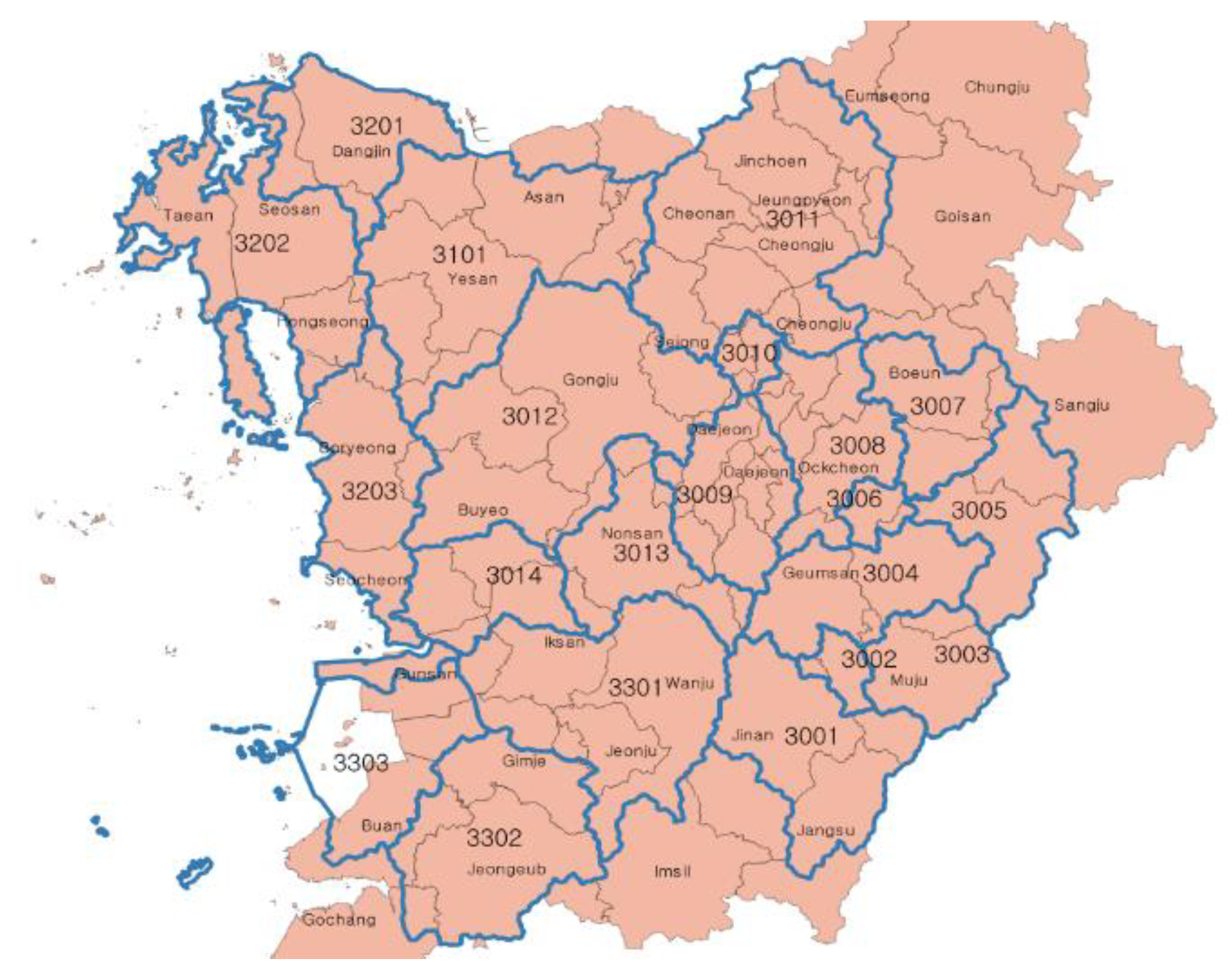
The study area is the Geumgang river (Figure 1), which covers the region 35.5–37.125° N and 126.0–128.0° E. The basin area is 17,925 km2, and the total river length is 36,142 km [23]. The study area comprises 21 sub-basins, and the basin areas of individual sub-basins range from 127.7 to 1843.7 km2. Additionally, the study area includes four multipurpose dams (Yongdam dam, Daecheong dam, Boryeong dam, and Buan dam) and 27 large-scale reservoirs with an effective reservoir capacity exceeding 5 million m3 for supplying water for agriculture as well as 2300 small reservoirs. In large cities with a population exceeding 500,000, such as Daejeon, Cheongju, Jeonju, and Cheonan, the household water demands are high, and several water-demanding places are present in national industrial complexes such as Gunsan and Asan. Furthermore, agricultural water demand stems from paddy fields and farm fields, accounting for about a quarter of the total basin area. Since the water demand for large cities, industrial complexes, and agricultural areas can be simultaneously simulated in the water balance model with various water supply facilities, the Geumgang river was selected as the study area.
The available data for this study are summarized in Table 1. The meteorological data recorded by weather stations from 1967 to 2015 were collected through the Water Resources Management Information System. RCP scenario data projected from 2011 to 2100 were collected from the Korea Metropolitan Administration. The acquired data were obtained from HadGEM3-RA, which is a regional climate model based on the atmospheric component of the Earth system model developed by the Met Office Hadley Centre, i.e., HadGEM3. To simulate the data with a spatial resolution of 0.125° in the Korean Peninsula area, the dynamic downscaling method was adopted for the four RCP scenarios (RCP 2.6, 4.5, 6.0, and 8.5), which are labeled as a possible range of radiative forcing values in the year 2100 (2.6, 4.5, 6.0, and 8.5 W/m2, respectively).
3. Methods
3.1. Conceptual Model (Water Balance Analysis)
To assess water shortages in the study area, the water system, including all sub-systems in the basin, needs to be analyzed. A water system can be defined as an entity extending over a geographical area, including all watersheds and groundwater recharge areas together with all water consumption centers and ecosystems associated with the processes occurring in natural (abiotic or biotic) and human sub-systems [27]. In the water system analysis, details of each sub-basin, e.g., rainfall-runoff characteristics, reservoir operation, and the lag time required for groundwater recharge after rainfall, can be included. Consequently, the analysis results can predict the affected areas and their amount of water shortage in each sub-basin. Herein, the water balance analysis conducted on the National Water Resources Plan (2001–2020) in Korea (hereafter referred to as the “National Plan”) [28] is first briefly explained and then the improvements for water supply and demand analysis are suggested for drought forecasting.
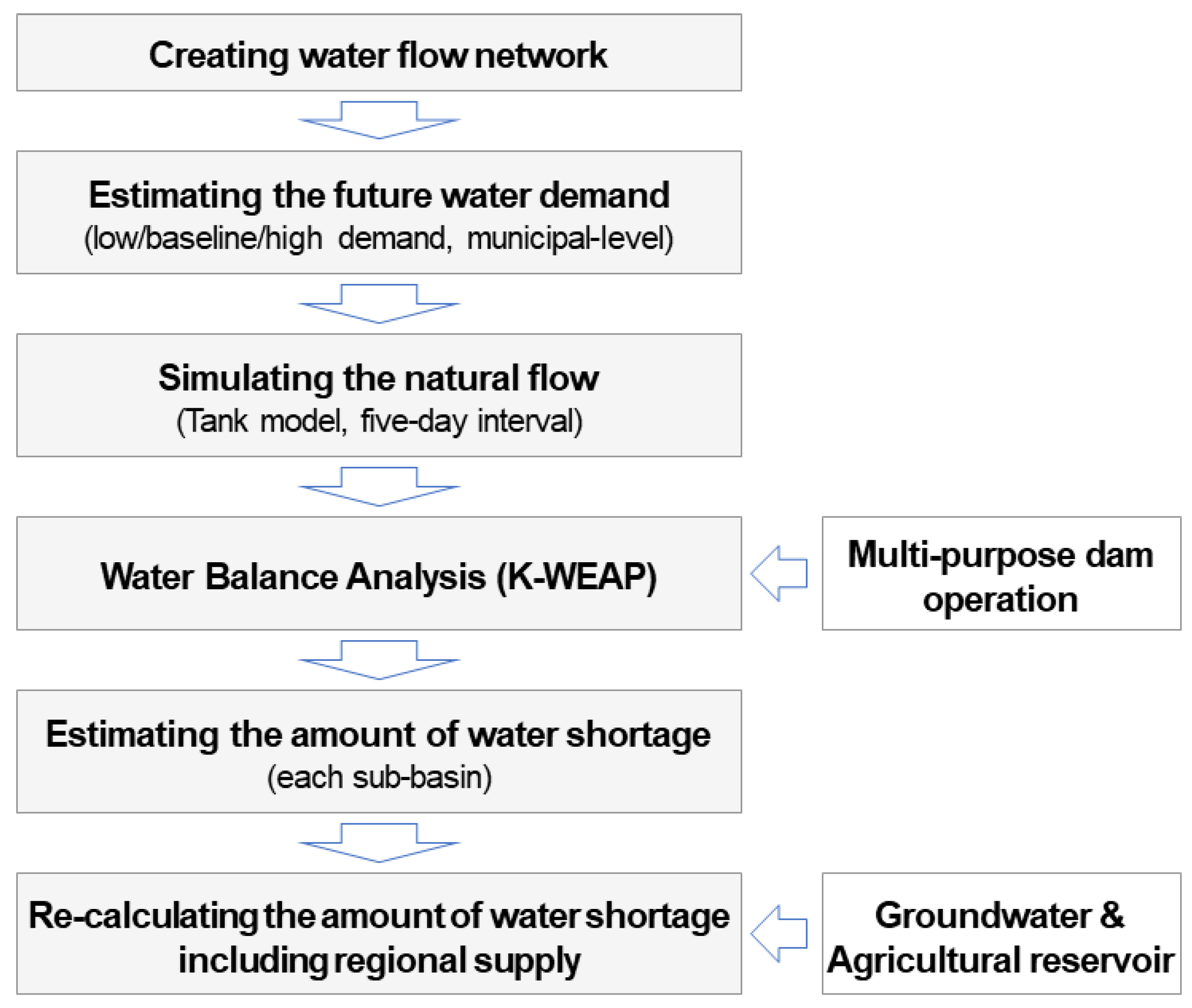
A National Plan is frequently prepared for developing detailed plans for water supply facilities. Figure 2 displays the water balance analysis process in the National Plan. For the 117 sub-basins in Korea, existing supply water sources (dams, reservoirs, groundwater, etc.), including natural flows, are compared with future water demand (household, industrial, agricultural, and ecological) to predict the probable water shortage. The amount of supply from natural flow is simulated using the Tank model with four serially connected tanks. The future water demand is estimated for each municipal-level district for low, baseline, and high demand cases for the year 2025, and the baseline demand is adopted herein. Since the National Plan aims to roughly determine the water shortage that can occur in the event of the worst drought for each major river basin, several assumptions are made in the analysis for convenience. However, these assumptions should be improved for drought forecasting in each sub-basin.
3.1.1. Improvement of Water Demand Analysis
In the National Plan, the water demand in each sub-basin is calculated as the district area ratio between the total area of each district and the area of the district included in the sub-basin, given by Equation (2), under the assumption that the water demands for household, industry, and agriculture are evenly distributed within an administrative district. However, mountainous, agricultural, industrial, and residential areas tend to be densely located in specific areas because of suitable natural conditions for agricultural and urban developments. Thus, the calculated demand for each sub-basin may differ from the actual amount of water demand.
Here, represents the total water demand in each sub-basin , is the total water demand (for household, industrial, and agricultural) in the administrative district , is the total area of , and is the area of included in sub-basin .
To improve the water demand estimation in each sub-basin, this study adopts the 2015 Population Census data (Eup/Myeon/Dong level, which is the lowest level of administrative divisions in Korea) and the GIS format of land use data (1:25,000) shown in Table 1. The population of the administrative districts and the areas of agricultural and industrial land in each sub-basin were used as weights to calculate the water demand for each sub-basin as follows.
Here, is the total area of a specific region (agricultural or industrial) or total population in the administrative district , and is the area of a specific region (agricultural or industrial) included in sub-basin out of the total area in the administrative district or the population in sub-basin out of the total population in the administrative district .
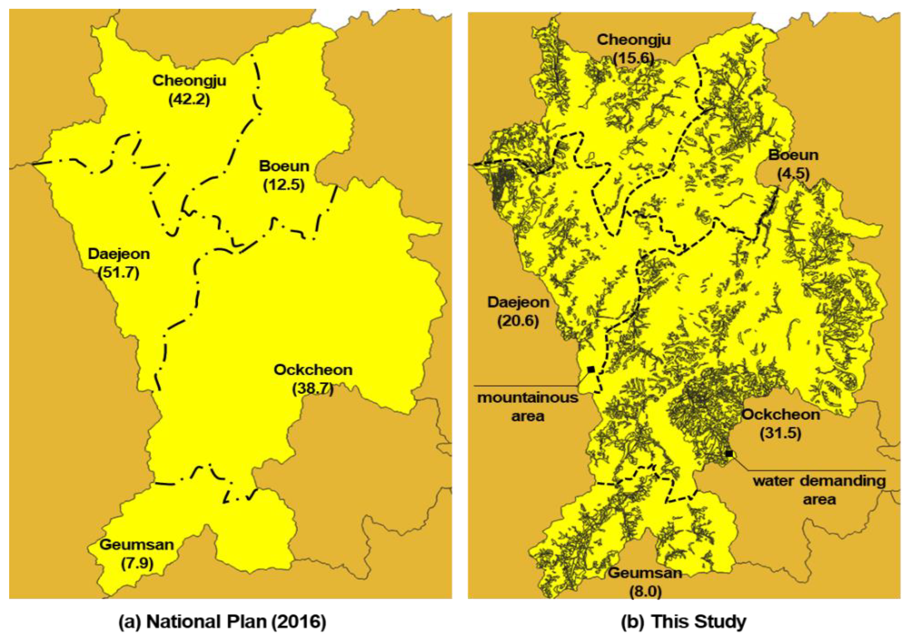
In the water demand calculation for all 21 sub-basins via both the existing method and the improved method, the water demand in five sub-basins is at a level of significant difference (the estimation in the improved method is more than 20% higher or lower than that in the existing method) and that in six sub-basins is at a level of moderate difference (the estimation in the improved method is more than 10–20% higher or lower than that in the existing method). Figure 3 describes the case of sub-basin 3008, exhibiting the maximum difference in demand estimation; a big portion of the watershed area is located upstream of the Daecheong dam, including mountainous and inundated areas. However, metropolitan cities such as Daejeon and Cheongju cover a large part of the watershed area, and therefore, the National Plan estimated an annual water demand of 153 million m3. However, the improved method estimated a sharply reduced value of 80 million m3.
Furthermore, the improved method separately simulates the water demand of household and industrial areas for each administrative district in the sub-basin to overcome the difficulty in calculating the water shortage for each district in the National Plan. Moreover, it includes the water demand in rainfed areas in the water shortage estimation with all water supply sources and the demand in the actual conditions, which is not included in the analysis of the National Plan.
3.1.2. Improvement of Water Supply Analysis
As shown in Figure 2, the National Plan does not include the regional water supplies from agricultural reservoirs and groundwater in the water balance analysis model, which can cause an underestimation of the water shortage amount [29,30]. Therefore, herein, groundwater for different consumers (household, agricultural, and industrial) is separately included in the analysis model. Furthermore, the integrated agricultural reservoir whose effective capacity is the same as the capacity of all reservoirs in each sub-basin is included in the analysis. Additionally, the improved method considers the location and capacity of intakes and sewage treatment plants in the water balance analysis. Therefore, the water intake and return within a sub-basin boundary and the water conveyance to neighboring sub-basins can be simulated using the improved model, whereas such processes cannot be simulated using the method in the National Plan.
3.1.3. MODSIM-DSS Model
Herein, the MODified SIMyld-Decision Support System (MODSIM-DSS) model is used for water balance analysis. This model was developed by Prof. Labadie of the Colorado State University by modifying SIMYLD, a network model developed by the Department of Water Resources Development (in 1972) in Texas, USA [31]. The model can reproduce the actual hydrological characteristics of the water system of the study area through the links and arcs connecting nodes (storage node, nonstorage node, demand node, and flowthru node) provided by the MODSIM-DSS model. The MODSIM-DSS model optimizes the flow rate in the links such that the cost incurred at all links during the calculation time () is minimized, which can be expressed as
Here, represents the cost, weight, or priority in link , represents the flow rate in link , and represents all links contained in the network.
The calculation constraints in each node can be expressed as follows:
Here, is the outgoing link from node , is the inflow link to node , is the demand of node at time , and and are the lower and upper limits, respectively, in link at time . Equation (5) is identical to the water balance equation (the total amounts of inflow and outflow at any node are the same), and Equation (6) is a physical condition that constrains the upper and lower limits of the flow in all the links.
In the optimization process involving Equations (4)–(6), the initial value of the flow vector is assumed and the dependent variables , , and are calculated based on the initial values. Then, the Lagrangian relaxation algorithm, which exhibits very fast convergence compared to existing linear programming, is used to iteratively calculate the priority or cost in each node and link until the values of the dependent variables converge. Subsequently, the optimal distribution of the water resources can be determined.
3.2. Data-Driven Model (Deep Neural Networks)
The first part of the methodology highlights the improvements in the water balance analysis, which is suitable for drought forecasting in the target watershed, and a method to quantitatively assess the risk of drought based on the water shortage amount. Advantageously, this method can spatially and temporally determine the drought risk, but considerable input data are required for each sub-basin for the assessment. Particularly, the water supply varies depending on the annual hydrologic and meteorological conditions. The amount of water available in the future can be estimated when the daily rainfall and evapotranspiration data over the next 1–3 months are obtained from the weather forecasting model. Considering the estimation uncertainty in the weather forecasting model, the water shortage with the natural flow needs to be determined from various scenarios (wet–normal–dry). This process can hinder prompt decision-making since it is complex and computationally intensive.
To promptly afford drought forecasts under various weather conditions, a DNN model based on the quantitative drought risk assessment is adopted herein. For the training and validation processes of the data-driven model, more than hundreds of data are required. According to Lee and Kim [32], when droughts that occurred in Korea from 1976 to 2010 were analyzed by SPI, the duration of each drought ranged from 2 to10 months, and in very few cases, two droughts occurred in a year. Only 49 years of data from 1967 to 2015 are available, and this is insufficient for training the drought forecasting model to derive a reliable outcome. Previous studies have developed alternative methods to extend the number of available data for the drought assessment. One study analyzed a tree-ring chronology network and converted it into the Palmer Severity Drought Index [33]. Furthermore, another study used rainfall data officially recorded by government agencies from the 18th to the 20th century in Korea to compare the drought risks in the past and present [34]. Herein, RCP scenarios are regarded as an event that may occur in the future, and a total of 360 years of data (4 scenarios × 90 years (2011–2100)) are additionally applied to extend the range of severe drought cases in the model training. Thus, we overcome the reliability issue stemming from the limited number of data in the past observation series.
The procedure for constructing an optimal DNN model for each sub-basin with past observation data and RCP scenarios (RCP 2.6, 4.5, 6.0, and 8.5) is as follows. First, the observation data and RCP scenario data are used in a previously constructed water balance analysis model, and the annual water shortage in the study area is calculated for each sub-basin. Second, to include the estimated water shortage as a dependent variable in the deep learning model, the water shortage data are rescaled to a range between zero and one by either normalization between the maximum and minimum values of the available data or a standardization with the average and standard deviation. This rescaling process limits the influence of large-scale variables in the training process of the DNN model and prevents the model from falling to a local minimum. However, the annual water shortage calculated in the water balance analysis tends to be a right-skewed distribution, indicating that moderate droughts frequently occur and extreme droughts rarely occur. Therefore, the calculated water shortage data need to be appropriately rescaled. Otherwise, the rescaled data cannot be evenly distributed in the range between zero and one. Herein, the generalized extreme value distribution in Equation (7) is adopted to rescale the amount of water shortage () to afford a non-exceedance probability (, 0–1).
Here, is the annual water shortage (in thousand cubic meters), is the shape parameter, is the scale parameter, and is the location parameter.
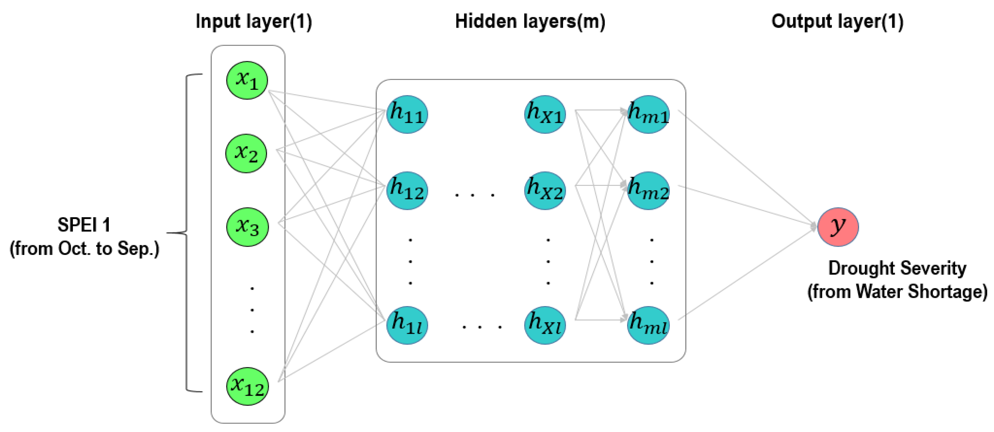
The independent variable of the DNN model is the 12 values of SPEI 1 (from October of the previous year to September of the present year), as shown in Figure 5. The input variable (SPEI 1) is rescaled to a range between zero and one by the non-exceedance probability of the normalized standard distribution to maintain the same scale in the input and output of the DNN model. A total of 45 models are trained by varying the number of hidden layers (three, four, and five layers; three cases), the number of nodes (30, 40, and 50 nodes; three cases), and the number of epochs (30, 60, 90, 120, and 150 epochs; five cases).
The training process involves a back-proposition algorithm where the weight is adjusted according to Equations (8) and (9) to minimize the cost functions of the predicted value () and observed value () in the output layer using the activation function [35].
Here, and represent the observed and predicted values at the -th node of the output layer, denotes the weight between the -th node of the previous layer and the -th node of the next layer in the -th model learning, and denotes the learning rate.
Finally, past observation data (1967–2015, 49 years), which are not used in the training process, are input into the 45 trained DNN models. Between the predicted water shortage through the trained model and the estimated water shortage through water balance analysis, the model displaying the best performance is selected as the optimal DNN for drought forecasting in each sub-basin. The mean squared error (MSE) and correlation coefficient are used as indicators to determine the model performances. Figure 6 describes the entire process to develop an optimal DNN model for drought forecasting in each sub-basin.
4. Results
4.1. Drought Assessment
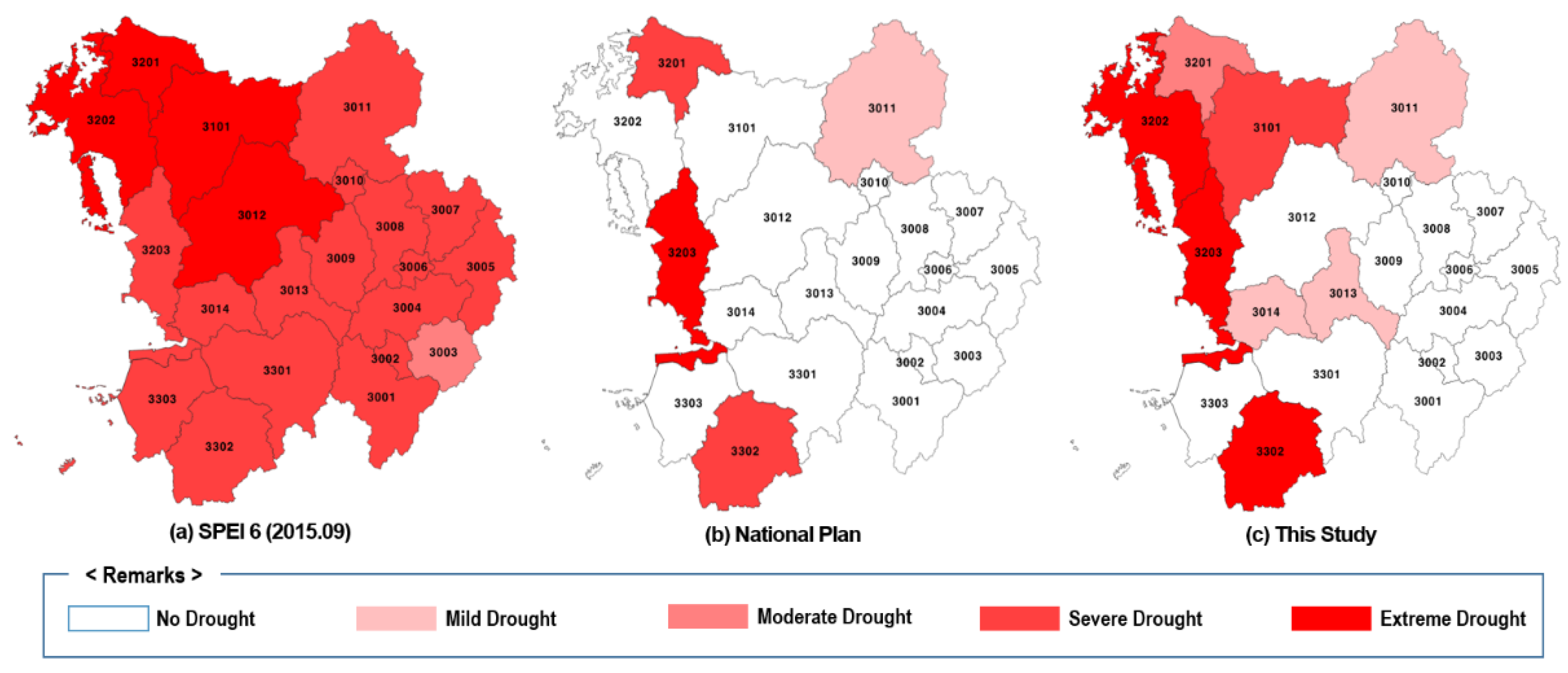
In the drought assessment with observation data for 49 years (1967–2015), the worst water shortage was estimated in the year 2015. For the worst year, the annual water shortage determined from the National Plan and the improved method proposed herein were compared in terms of a meteorological drought index (SPEI 6), as described in Figure 7. For the meteorological drought index (SPEI 6) for September 2015, it was difficult to ascertain which area should be first considered; apart from the sub-basin 3003, the entire study area exhibited severe or extreme levels of drought. However, the hydrological drought cases from the water balance analysis model provide information about the affected location and the expected water shortage amount. Table 3 shows the criteria for classifying drought severity based on water shortage; the criteria were determined by applying the severity of an event in SPI to the water shortage performed with the observation data for 49 years for each sub-basin.
Comparison of the drought assessment results between the National Plan and the improved model showed that a severe or extreme level of water shortage was predicted in four areas by the improved model and in only three areas by the National Plan. Particularly, in sub-basins 3101 and 3202, no shortage was expected according to the National Plan, while the analysis with improvements indicated a severe or extreme level of drought. Such difference in the impacted areas stemmed from the water demand in the rainfed farm field, which was not considered in the National Plan. Furthermore, in sub-basin 3203, the National Plan predicted a water shortage of 54 million m3 while the improved method predicted a significantly reduced a water shortage of 31 million m3. Such a reduction resulted from the improvement in the demand estimation method; 35 million m3 of agricultural water demand was decreased in the sub-basin 3203.
The differences in the afflicted areas and their severity between the two methods show that the improved method of this study more accurately simulates the drought damage than the National Plan. The improved method requires calibration through comparison with the recorded drought damage. However, the calibration was not performed herein owing to insufficient detailed data on the water shortage in the affected areas in the drought damage investigation reports published by the Korean government [36,37,38]. When sufficient data are available, additional studies need to be performed for model calibration.
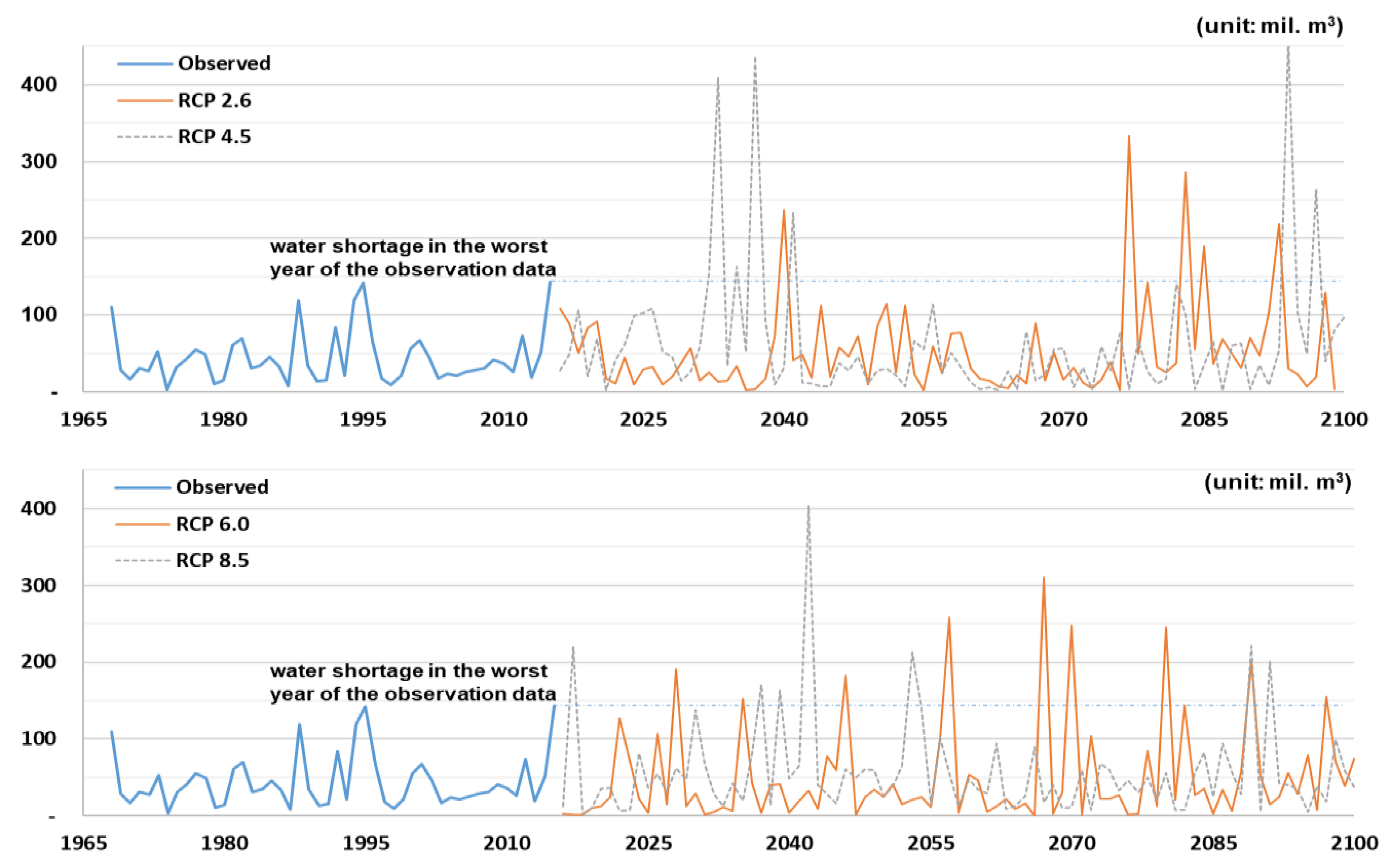
The annual water shortages in the case of the past observation data and RCP scenarios are shown in Figure 8. In the observation data for the past 49 years, the worst drought was recorded in 2015 with water shortage of 143 million m3, but the maximum water shortage reached 310–458 million m3 in each scenario. In each of the RCP scenarios, the water shortage exceeded the value in the year 2015 by 7–10 times, and 32 extreme drought cases were additionally included in the training of the DNN model for drought forecasting. This can contribute to the reliable prediction of the expected damage in the drought events, exceeding the recorded range of past observation data. This is similar to the improvement of the reliability of the peak discharge estimate for extreme flood events by adding extreme values from the regional frequency analysis.
4.2. Drought Forecasting
As previously described, the rescaled values of SPEI 1 and annual water shortage from the water balance analysis were used as the independent and dependent variables, respectively, in the DLL model’s training. For each of the sub-basins, models with 45 hyperparameter combinations were constructed, and training and validation processes were sequentially performed for each model to minimize the cost function between the target and predicted values. As the number of epochs was increased from 30 to 150, for each epoch, nine models were trained and validated with different values of hidden layers and nodes for each hidden layer. Figure 9 presents the cases with the best validation results for each epoch after the training and validation processes in sub-basins 3101 and 3202. The figure displays the performance of the trained models along with the MSE and the correlation between the value estimated from the DNN model and the target value (results from the MODSIM-DSS model). Both the values indicate that the model constructed through training and validation is a solid representation of the drought situations: the correlation coefficient was higher than 0.8 in all cases, and the MSE had an accuracy of 0.02–0.03.
Then, the optimal DNN for each sub-basin was determined using the meteorological data from 1967 to 2015 (49 years), which were not employed in the previous stage. Of the 45 models, the model exhibiting the minimum MSE value between the inferred and target values (the annual water shortage from the MODSIM-DSS model) was selected as the optimal model. In the sub-basins 3101 and 3202, the model with 150 epochs, four hidden layers, and 40 nodes for each hidden layer and that with 60 epochs, five hidden layers, and 50 nodes for each hidden layer were selected as the optimal model, respectively. Figure 10 describes the water shortage estimated from the past observation data in the optimal model, which are displayed with the values predicted by the water balance analysis as a time series. The estimated water shortage agrees with the target value in the two sub-basins, and the occurrences of severe water shortages were correctly predicted (e.g., in 1988, 1995, and 2015).
Table 4 displays the contribution of the RCP scenarios to the DNN model reliability in comparison with Case 1, where the past data from 1967 to 2005 were repeatedly used for training and validation of the DNN models. For Case 2, the optimal DNN model previously selected was adopted. Apart from the available data for model training and validation, model training with several hyperparameter cases and the selection of the optimal DNN model among the trained models were identical to those for the RCP scenario case. Furthermore, to compare the training performance on the same basis, the past observation data from 2006 to 2015 were used in the two models and the inference results of both the models were compared with the water shortage amounts derived from the water balance analysis. Table 4 shows that the results of the training and validation process did not significantly differ between Case 1 and Case 2. However, in the inference results with data from 2006 to 2015, for the model trained with a limited number of past observation data, MSE significantly increased and the correlation coefficient decreased, which was not observed for the model trained with the RCP scenarios. This comparison result shows that the construction of a model with considerably more data can afford more reliable drought forecasting results.
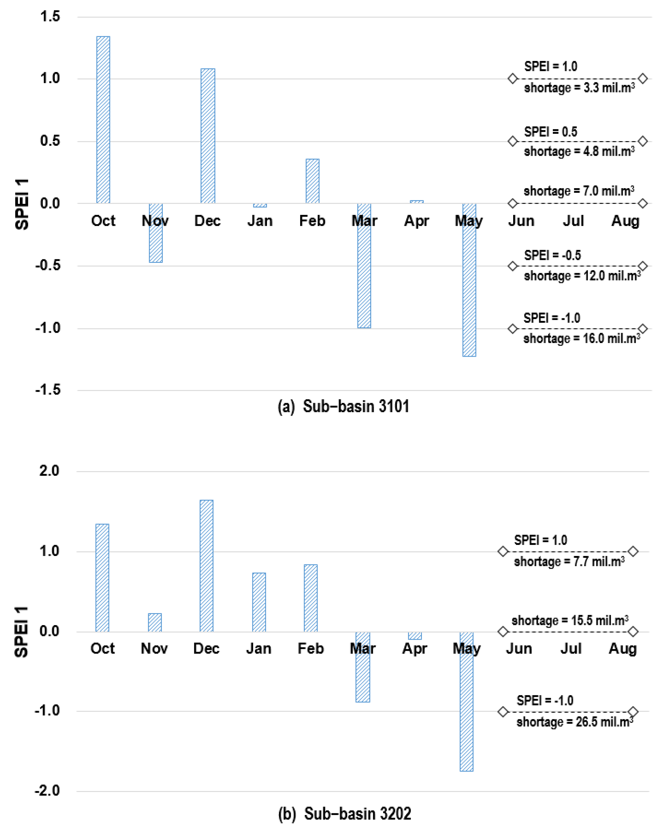
Through the aforementioned process, an optimal DNN model was constructed for each sub-basin. Thus, if the weather data observed from October of the previous year and the weather forecasting data in the near future are prepared in the form of monthly SPEI indices, water shortages for the following period can be predicted. Currently, the National Drought Information Portal of Korea declares the drought index of the past six months and forecasts future droughts in units of month (1 month) or season (3 months) [39]. Therefore, the past observation and three-month weather forecast data can be used for drought forecasting. The results of the application of various meteorological conditions to the optimal DNN model for sub-basins 3101 and 3202 in the year 2015 are shown in Figure 11. In the drought situation occurring from October 2014 to May 2015, highlighting the lack of rainfall in March and May associated with seasonal rainfall fluctuations, is notable. The monthly rainfall that occurred in March and May was just 42% and 32%, respectively, of the average monthly rainfall in the observation data. Specifically, since the high demand period for agricultural water usually starts from May because of rice seeding in paddy fields, water needs to be supplied from agricultural reservoirs to meet the demand. However, the precipitation during these periods was not sufficient to refill the reservoirs. Therefore, this was the main reason for the most severe drought from June to August (the crop growth period) in the past observation cases.
In the annual water shortage forecasting in sub-basins 3101 and 3202, various SPEI indices in the range from −1 to 1 were used in the optimal DNN model for three months from June to August. The optimal DNN model showed that water shortages may occur in the range of 3–16 and 8–27 million m3 in sub-basins 3101 and 3202, respectively. In sub-basin 3101, an SPEI index between −0.6 and −0.9 was recorded during the period, and the water balance analysis model predicted a water shortage of 13 million m3. In sub-basin 3202, an SPEI index between −0.9 and −1.4 was recorded, and the water balance model predicted a water shortage of 30 million m3. These results are clearly in good agreement, further demonstrating the reliability of the optimal DNN model in forecasting drought damage. Therefore, this is a useful tool for a decision maker to determine the water shortage and the required amount of rainfall to reduce the damage. This model can be used to proactively formulate water-saving measures and water supply measures through diversion from nearby basins before the on-set of extreme droughts.
5. Discussion and Conclusions
Herein, a risk-based drought management system was presented for decision makers to formulate countermeasures for upcoming drought damage [14]. The following requirements should be satisfied to support decision makers in forecasting drought damage. First, the spatial extent considered for forecasting should include all water systems (all the water consumptions and all sources of water supply) in the area. This assessment of water shortages in the water system can contribute toward identifying both afflicted areas and their severity. The assessment results, rather than being expressed as complex statistical figures, should be expressed as quantitative values, such as the amount of water shortage directly resulting from an existing drought and the amount of precipitation required for the damage mitigation. Finally, rather than putting effort into recovery after disaster occurs, forecasting should be frequently performed with limited information and numerous weather forecasting scenarios, and the result should be delivered to decision makers well before drought onset. To satisfy these requirements, this study proposes the methodology for a drought forecasting system to couple the water balance analysis model, which is a physical/conceptual model, and the DNN model, which is a data-driven model.
In drought assessment, based on the analysis method currently used in the National Plan, several improvements were proposed to include all the water systems and examine the actual situation. Moreover, the demand estimation method in the sub-basin was improved by applying the GIS format of land use and the population census data, and the agricultural demand in the rainfed area was included to accurately estimate the actual water demand. In terms of water supply, both agricultural reservoirs and confined aquifers as well as intake and sewage treatment facilities were included to simulate water supply and return within the sub-basin boundary. Due to these improvements, the affected areas and their water shortage was simulated in the model; thus, the model is suitable for drought forecasting at the sub-basin level. In previous studies, to improve the water balance analysis model in the National Plan, similar approaches have been suggested, such as including agricultural reservoirs and agricultural demand in the rainfed area in the analysis [30,40,41]. However, to our knowledge, no previous study has adopted the GIS format of land use and the population census data to estimate the water demand in each sub-basin area. Of the 21 sub-basins in the study area, the water demand in 11 sub-basin areas estimated by the current method and the improved method was at a level of significant or moderate difference. Additionally, the water balance analysis model is generally adopted to calculate the required volume of the water management facility to prevent water shortage under the future water demand conditions and to simulate the variation of the water shortage due to climate change [42,43,44]. However, herein, the water balance analysis was used for the drought damage forecasting to simultaneously identify the afflicted areas and their water shortage. For the drought case of the year 2015, the water balance analysis reliably indicated the four severely impacted areas based on the amount of water shortage, while the meteorological drought index indicated that 20 sub-basins were severe drought areas.
In the drought forecasting with the DNN model, observation data from the past 50 years were not sufficient to train the model. As an alternative measure, RCP scenarios were assumed to represent possible weather events in the future. Of the 360 years of the water shortage resulting from the four RCP scenarios, 32 cases of water shortage exceeded the value of the worst drought year obtained from the past observation data. When sufficient data from extreme drought cases were considered, the performance of the model training and validation was within an acceptable range, and optimal DNN models were derived for each sub-basin. In previous studies, the tree-ring chronology network and the recorded rainfall data from the 18th to 19th century were adopted for reliability in the extreme drought analysis [31,32,45]. Herein, the RCP scenarios were included in the training process of the DNN model, which significantly increased the correlation coefficient of 0.82–0.83 in comparison with the correlation coefficient of 0.52–0.63 in the model training with a limited number of the observed data.
Herein, for the drought event in 2015, the optimal DNN model exhibited reliable drought damage forecasting with various meteorological conditions for the next several months. Data-driven stochastic methods, such as artificial neural networks and autoregressive integrated moving average models, are commonly employed for drought forecasting [21,46,47,48]. Additionally, the meteorological and hydrological models are employed together for hydrological drought forecast [49,50,51]. However, none of these previous studies have considered coupling the water balance model and DNN model. Since the coupled model proposed herein can deliver reliable and prompt predictions of the drought damage, it can contribute to the continuous analysis of the expected water shortage and the amount of rainfall for the following period, which can assist in formulating proactive measures for forecasted droughts.
In a follow-up study, the reliability of the analysis results needs to be improved by calibrating the water balance analysis model, which was not performed in this study because of the lack of current drought damage survey data. Moreover, to improve the consistency between the values predicted through the optimal DNN model and the values calculated through the water balance analysis, additional climate change scenarios from other organizations need to be adopted in the training and validation process of the DNN model. Additionally, other variables need to be considered as independent variables for the DNN model, such as the number of days of rainfall in each month and the average rainfall intensity. Finally, since recognizing the cause of the predicted results from the DNN model is difficult, we propose that a preliminary analysis should be performed of the threshold or weather patterns that might cause an extreme drought event since it will improve the understanding of the cause.
Author Contributions
Conceptualization, O.-J.J. and H.-T.M.; methodology, O.-J.J.; formal analysis, O.-J.J.; investigation, O.-J.J. and H.-T.M.; resources, O.-J.J.; data curation, O.-J.J.; writing—original draft preparation, H.-T.M.; writing—review and editing, Y.-I.M.; supervision, Y.-I.M.; project administration, Y.-I.M.; funding acquisition, Y.-I.M. All authors have read and agreed to the published version of the manuscript.
Funding
This work was generally supported by the University of Seoul.
Institutional Review Board Statement
Not applicable.
Informed Consent Statement
Not applicable.
Data Availability Statement
Not applicable.
Conflicts of Interest
The authors declare no conflict of interest.
References
- World Meteorological Organization (WMO). Special Environment Report No. 5; WMO: Geneva, Switzerland, 1975; pp. 17–25. [Google Scholar]
- Hong, W.; Wilhite, D.A. An operational agricultural drought risk assessment model for Nebraska, USA. Nat. Hazards 2004, 33, 1–21. [Google Scholar]
- Mishra, A.K.; Singh, V.P. A review of drought concepts. J. Hydrol. 2010, 391, 202–216. [Google Scholar] [CrossRef]
- Zargar, A.; Sadiq, R.; Naser, B.; Khan, F.I. A review of drought indices. Environ. Rev. 2011, 19, 333–349. [Google Scholar] [CrossRef]
- McKee, T.B.; Doesken, N.J.; Kleist, J. The relationship of drought frequency and duration to time scales. In Proceedings of the 8th Conference on Applied Climatology, Anaheim, CA, USA, 17–22 January 1993. [Google Scholar]
- Palmer, W.C. Meteorological Drought. Research Paper No. 45; USA Department of Commerce Weather Bureau: Washington, DC, USA, 1965; pp. 1–58. [Google Scholar]
- Vicente-Serrano, S.M.; Begueria, S.; Lopez-Moreno, J.I. A multi-scalar drought index sensitive to global warming: The Standardized Precipitation Evapotranspiration Index. J. Clim. 2010, 23, 1696–1718. [Google Scholar] [CrossRef] [Green Version]
- Tsakiris, G.; Vangelis, H. Establishing a drought index incorporating evapotranspiration. Eur. Water 2015, 9, 3–11. [Google Scholar]
- Tsakiris, G. Drought risk assessment and management. Water Resour. Manag. 2017, 31, 3083–3095. [Google Scholar] [CrossRef]
- Intergovernmental Panel on Climate Change (IPCC). Climate Change 2014: Impacts, Adaptation, and Vulnerability; Contribution of Working Group II to the Fifth Assessment Report of the IPCC; Cambridge University Press: Cambridge, UK, 2014; p. 1048. [Google Scholar]
- Kim, J.S.; Park, S.Y.; Hong, H.P.; Chen, J.; Choi, S.J.; Kim, T.W.; Lee, J.H. Drought risk assessment for future climate projections in the Nakdong River Basin, Korea. Int. J. Climatol. 2020, 40, 4528–4540. [Google Scholar] [CrossRef]
- Pei, W.; Fu, Q.; Liu, D.; Li, T.; Cheng, K.; Cui, S. A novel method for agricultural drought risk assessment. Water Resour. Manag. 2019, 33, 2033–2047. [Google Scholar] [CrossRef]
- Kuntiyawichai, K.; Wongsasri, S. Assessment of drought severity and vulnerability in the Lam Phaniang River Basin, Thailand. Water 2021, 13, 2743. [Google Scholar] [CrossRef]
- Ortega-Gaucin, D.; Ceballos-Tavares, J.A.; Sánchez, A.O.; Castellano-Bahena, H.V. Agricultural drought risk assessment: A spatial analysis of hazard, exposure, and vulnerability in Zacatecas, Mexico. Water 2021, 13, 1431. [Google Scholar] [CrossRef]
- Yan, D.; Weng, B.; Wang, G.; Wang, H.; Yin, J.; Bao, S. Theoretical framework of generalized watershed drought risk evaluation and adaptive strategy based on water resources system. Nat. Hazards 2014, 73, 259–276. [Google Scholar] [CrossRef]
- Wilhite, D.A.; Svoboda, M.D. Drought Early Warning Systems in the Context of Drought Preparedness and Mitigation. In Early Warning Systems for Drought Preparedness and Drought Management; WMO: Geneva, Switzerland, 2000; pp. 1–21. [Google Scholar]
- Nam, W.H.; Choi, J.Y.; Yoo, S.H.; Jang, M.W. A decision support system for agricultural drought management using risk assessment. Paddy Water Environ. 2012, 10, 197–207. [Google Scholar] [CrossRef]
- Quijano, J.A.; Jaimes, M.A.; Torres, M.A.; Reinoso, E.; Castellanos, L.; Escamilla, J.; Ordaz, M. Event-based approach for probabilistic agricultural drought risk assessment under rainfed conditions. Nat. Hazards 2015, 76, 1297–1318. [Google Scholar] [CrossRef]
- Yue, Y.; Wang, L.; Li, J.; Zhu, A. An EPIC model-based wheat drought risk assessment using new climate scenarios in China. Clim. Change 2018, 147, 539–553. [Google Scholar] [CrossRef]
- Naumann, G.; Spinoni, J.; Vogt, J.V.; Barbosa, P. Assessment of drought damages and their uncertainties in Europe. Environ. Res. Lett. 2015, 10, 1–14. [Google Scholar] [CrossRef]
- Lim, J.D.; Yang, J.S. Possibility analysis of future droughts using long short term memory and standardized groundwater level index. J. Korea Water Resour. Assoc. 2020, 53, 131–140. [Google Scholar]
- Blauhut, V.; Gudmundsson, L.; Stahl, K. Towards pan-European drought risk maps: Quantifying the link between drought indices and reported drought impacts. Environ. Res. Lett. 2015, 10, 1–10. [Google Scholar] [CrossRef]
- Observed Meteorological Data. Available online: http://www.wamis.go.kr (accessed on 22 October 2020).
- RCP Scenarios. Available online: http://www.climate.go.kr (accessed on 5 November 2020).
- Population Census in 2015. Available online: https://kostat.go.kr/portal/eng/index.action (accessed on 5 November 2020).
- Land-Use Data (GIS Format). Available online: http://www.nsdi.go.kr/ (accessed on 14 November 2020).
- Tsakiris, G.; Nalbantis, I.; Vangelis, H.; Verbeiren, B.; Huysmans, M.; Tychon, B.; Jacquemin, I.; Canters, F.; Vanderhaegen, S.; Engelen, G.; et al. A system-based paradigm of drought analysis for operational management. Water Resour. Manag. 2013, 27, 5281–5297. [Google Scholar] [CrossRef]
- Ministry of Land, Infrastructure, and Transport (MOLIT). National Water Resources Plan (2001∼2020); Publication No. 11-1613000-001716-13; MOLIT: Sejong, Korea, 2016; pp. 198–233. [Google Scholar]
- K-Water. A Study on the Basic Plan for Water Management; Publication No. 11-B500001-000091-01; K-Water: Daejeon, Korea, 2008; pp. 233–287. [Google Scholar]
- Choi, S.J.; Kang, S.K.; Lee, D.R.; Kim, J.H. A study on water supply and demand prospects for water resources planning. J. Korean Soc. Hazard Mitig. 2018, 18, 589–596. [Google Scholar] [CrossRef] [Green Version]
- K-Water. K-MODSIM Manual; Ver. 1.1; K-Water: Daejeon, Korea, 2007; pp. 1–40. [Google Scholar]
- Lee, J.H.; Kim, C.J. Derivation of drought severity-duration-frequency curves using drought frequency analysis. J. Korea Water Resour. Assoc. 2011, 44, 889–902. [Google Scholar] [CrossRef] [Green Version]
- Cook, E.R.; Woodhouse, C.A.; Eakin, C.M.; Meko, D.M.; Stahle, D.W. Long-term aridity changes in the western United States. Science 2004, 306, 1015–1018. [Google Scholar] [CrossRef] [PubMed] [Green Version]
- Kim, J.E.; Yu, J.S.; Lee, J.H.; Kim, T.W. Drought risk analysis in Seoul using Cheugugi and climate change scenario based rainfall data. J. Korea Water Resour. Assoc. 2018, 38, 387–393. [Google Scholar]
- Neural Networks and Deep Learning. Available online: http://neuralnetworksanddeeplearning.com (accessed on 10 October 2020).
- Korea Institute of Civil Engineering and Building Technology (KICT). Investigating Report for the Drought in 1995; KICT: Goyang, Korea, 1995. [Google Scholar]
- Korea Rural Community Corporation (KRC). White Book for the Drought in 2012; KRC: Naju, Korea, 2012. [Google Scholar]
- MOLIT. Investigating Report for the Drought in 2015; MOLIT: Sejong, Korea, 2016. [Google Scholar]
- National Drought Information-Analysis Center(NDIC). Drought assessment and forecasting. In Response Guidebook for Drought Disaster; NDIC: Sejong, Korea, 2016; p. 117. [Google Scholar]
- Oh, J.H.; Kim, Y.S.; Ryu, K.S.; Bae, Y.D. Comparison and discussion of water supply and demand forecasts considering spatial resolution in the Han-river basin. J. Korea Water Resour. Assoc. 2019, 52, 463–473. [Google Scholar]
- Oh, J.H.; Kim, Y.S.; Ryu, K.S.; Jo, Y.S. Comparison and discussion of MODSIM and K-WEAP model considering water supply priority. J. Korea Water Resour. Assoc. 2019, 52, 505–514. [Google Scholar]
- Choi, S.J.; Lee, D.R.; Kang, S.K. Analysis of water supply capacity based on future various scenarios in Geum river basin. J. Korean Soc. Hazard Mitig. 2018, 19, 315–321. [Google Scholar] [CrossRef] [Green Version]
- Papadimos, D.; Demertzi, K.; Papamichail, D. Assessing lake response to extreme climate change using the coupled MIKE SHE/MIKE 11 Model: Case Study of Lake Zazari in Greece. Water 2022, 14, 921. [Google Scholar] [CrossRef]
- Ashu, A.B.; Lee, S.-I. Assessing climate change effects on water balance in a monsoon watershed. Water 2020, 12, 2564. [Google Scholar] [CrossRef]
- Hutton, P.H.; Meko, D.M.; Roy, S.B. Supporting restoration decisions through integration of tree-ring and modeling data: Reconstructing flow and salinity in the San Francisco estuary over the past millennium. Water 2021, 13, 2139. [Google Scholar] [CrossRef]
- Alsumaiei, A.A.; Alrashidi, M.S. Hydrometeorological drought forecasting in hyper-arid climates using nonlinear autoregressive neural networks. Water 2020, 12, 2611. [Google Scholar] [CrossRef]
- Myronidis, D.; Ioannou, K.; Fotakis, D.; Dörflinger, G. Streamflow and hydrological drought trend analysis and forecasting in Cyprus. Water Resour. Manag. 2018, 32, 1759–1776. [Google Scholar] [CrossRef]
- Belayneh, A.; Adamowski, J.; Khalil, B.; Ozga-Zielinski, B. Long-term SPI drought forecasting in the Awash River basin in Ethiopia using wavelet neural network and wavelet support vector regression models. J. Hydrol. 2014, 508, 418–429. [Google Scholar] [CrossRef]
- So, J.-M.; Lee, J.-H.; Bae, D.-H. Development of a hydrological drought forecasting model using weather forecasting data from GloSea5. Water 2020, 12, 2785. [Google Scholar] [CrossRef]
- Fundel, F.; Jörg-Hess, S.; Zappa, M. Monthly hydrometeorological ensemble prediction of streamflow droughts and corresponding drought indices. Hydrol. Earth Syst. Sci. 2013, 17, 395–407. [Google Scholar] [CrossRef] [Green Version]
- Sheffield, J.; Wood, E.F.; Chaney, N.; Guan, K.; Sadri, S.; Yuan, X.; Olang, L.; Amani, A.; Ali, A.; Demuth, S. A drought monitoring and forecasting system for sub-Sahara African water resources and food security. Bull. Am. Meteorol. Soc. 2014, 95, 861–882. [Google Scholar] [CrossRef]
Figure 1.
Study area of the Geumgang river.

Figure 2.
Process of water balance analysis in the National Plan.

Figure 3.
Comparison of the demand estimation between the National Plan and this study (unit: mil. m3/year): (a) water demand estimated by the district area included in each watershed; (b) water demand calculated by the areas demanding water (such as farm field, paddy field, and industrial area) based on the GIS analysis.

Figure 4.
Comparison of the flow network between the National Plan and the improved method of this study: (a) each node for agricultural demand and household and industrial demand is included in the water balance simulation of the National Plan; (b) one node for agricultural demand and separate nodes for household and industrial demand, aquifers, and reservoirs are included in the simulation of this study.

Figure 5.
DNN model structure for training and validation.

Figure 6.
Flow chart for developing an optimal DNN model for drought forecasting (AWS denotes the Annual Water Shortage).
Figure 6.
Flow chart for developing an optimal DNN model for drought forecasting (AWS denotes the Annual Water Shortage).

Figure 7.
Comparison of drought assessment between the National Plan and the improved method proposed herein: (a) meteorological drought assessment based on the SPEI6 index in Sep. 2015; (b) water shortage assessment adopting the National Plan’s methodology; (c) water shortage assessment adopting the improved method of this study.

Figure 8.
Annual water shortage in the case of the past observation data and RCP scenarios.

Figure 9.
Validation result after DLL model training for predicting the amount of water shortage. The model training performance for each epoch is presented with MSE and correlation coefficient in (a) sub-basin 3101 and (b) sub-basin 3202.
Figure 9.
Validation result after DLL model training for predicting the amount of water shortage. The model training performance for each epoch is presented with MSE and correlation coefficient in (a) sub-basin 3101 and (b) sub-basin 3202.

Figure 10.
Inference results of the optimal DNN models for predicting the water shortage amount. The target indicates the water shortage predicted from the water balance analysis model and the inferred indicates the value estimated from the optimal DNN model. The performance of the optimal DNN model is presented in (a) sub-basin 3101 and (b) sub-basin 3202.

Figure 11.
Amount of water shortage forecasted under different SPEI conditions of the 2015 drought case. The observed SPEI values from October 2014 to May 2015 were included in the optimal DNN model and the amount of water shortage was forecasted in May 2015 depending on the different SPEI scenarios between June 2015 and August 2015 in (a) sub-basin 3101 and (b) sub-basin 3202.


Table 1.
Available data for the study.
| Category | Available Data | Sources |
|---|---|---|
| Observed Meteorological Data | Rainfall, evapotranspiration
| Water Resources Management Information System [23] |
| RCP Scenario | RCP 2.6, 4.5, 6.0, and 8.5 Rainfall, maximum and minimum temperature, relative humidity, and wind velocity
| Korea Meteorological Administration [24] |
| Population | Population Census in 2015 (37 districts) | Korea National Statistical Office [25] |
| Land-use | GIS format (1:25,000, 37 districts) | National Spatial Data Infrastructure Portal [26] |
Table 2.
Summary of the improvements of the water balance analysis.
| National Plan | Improvements of This Study | ||
|---|---|---|---|
| Flow Network | Agricultural demand | One node in the sub-basin | One node in the sub-basin |
| Household and Industrial demand | One node in the sub-basin | Separate nodes for each district in the sub-basin | |
| Water Demand | Demand estimation | Equation. (2) adopted - household, agricultural, industrial : district area ratio | Equation (3) adopted - household : population living in the sub-basin - agricultural, industrial : related area in the sub-basin |
| Demand for the rainfed farming | Not included | Included | |
| Water Supply | Agricultural reservoir and confined aquifer | After the K-WEAP simulation, the water shortage is reduced as much as the supplies from both sources | Both supplies are included in the simulation |
| Intake and sewage treatment plant | Location and capacity are not considered | Location and capacity are considered in the simulation | |
| Simulation result | Annual water shortage | Water shortage in each simulation step | |
Table 3.
Drought warning criteria for meteorological drought and this study.
| Category | Mckee et al. (1993) [5] | This Study (Water Shortage) | |
|---|---|---|---|
| SPI | Severity of Event | ||
| Mild dryness | 0 to −0.99 | 1 in 3 years | 0–5 mil. m3/year |
| Moderate dryness | −1.00 to −1.49 | 1 in 10 years | 5–10 mil. m3/year |
| Severe dryness | −1.50 to −1.99 | 1 in 20 years | 10–30 mil. m3/year |
| Extreme dryness | over −2.00 | 1 in 50 years | over 30 mil. m3/year |
Table 4.
Comparison of the inference results between the models trained by the past data and RCP scenarios.
Table 4.
Comparison of the inference results between the models trained by the past data and RCP scenarios.
| Sub-Basin | Case | Process (Adopted Data) | MSE | Correlation Coefficient |
|---|---|---|---|---|
| 3101 | 1 | Training (Past, 1967–2005) | 0.019 | 0.791 |
| Inference (Past, 2006–2015) | 0.034 | 0.529 | ||
| 2 | Training (RCP, 2011–2100) | 0.017 | 0.837 | |
| Inference (Past, 2006–2015) | 0.018 | 0.826 | ||
| 3202 | 1 | Training (Past, 1967–2005) | 0.033 | 0.749 |
| Inference (Past, 2006–2015) | 0.033 | 0.630 | ||
| 2 | Training (RCP, 2011–2100) | 0.032 | 0.830 | |
| Inference (Past, 2006–2015) | 0.019 | 0.818 |
Publisher’s Note: MDPI stays neutral with regard to jurisdictional claims in published maps and institutional affiliations. |
© 2022 by the authors. Licensee MDPI, Basel, Switzerland. This article is an open access article distributed under the terms and conditions of the Creative Commons Attribution (CC BY) license (https://creativecommons.org/licenses/by/4.0/).
Share and Cite
MDPI and ACS Style
Jang, O.-J.; Moon, H.-T.; Moon, Y.-I. Drought Forecasting for Decision Makers Using Water Balance Analysis and Deep Neural Network. Water 2022, 14, 1922. https://doi.org/10.3390/w14121922
AMA Style
Jang O-J, Moon H-T, Moon Y-I. Drought Forecasting for Decision Makers Using Water Balance Analysis and Deep Neural Network. Water. 2022; 14(12):1922. https://doi.org/10.3390/w14121922
Chicago/Turabian StyleJang, Ock-Jae, Hyeon-Tae Moon, and Young-Il Moon. 2022. "Drought Forecasting for Decision Makers Using Water Balance Analysis and Deep Neural Network" Water 14, no. 12: 1922. https://doi.org/10.3390/w14121922
Note that from the first issue of 2016, this journal uses article numbers instead of page numbers. See further details here.