
Impact of Climate Change on Soil Water Content in Southern Saskatchewan, Canada


1
Prairie Adaptations Research Collaborative, University of Regina, Regina, SK S4S 0A2, Canada
2
Environmental Systems Engineering, University of Regina, Regina, SK S4S 0A2, Canada
*
Author to whom correspondence should be addressed.
Water 2022, 14(12), 1920; https://doi.org/10.3390/w14121920
Submission received: 9 May 2022
/
Revised: 7 June 2022
/
Accepted: 10 June 2022
/
Published: 14 June 2022
(This article belongs to the Section Soil and Water)
Abstract
:The main objective of this research was to understand the effects of climate change on soil water content (SWC) across the Qu’Appelle River basin in southern Saskatchewan, Canada. The Soil and Water Assessment Tool (SWAT) and output from 11 high-resolution (0.22°) regional climate models (RCM) were used over three 30-year periods: the near future (2021–2050) and distant future (2051–2080) and the historical reference (1975–2005). The RCM data are from the CORDEX North American domain, which employs the RCP8.5 high-emission scenario. SWC was modeled at the hydrological response units (HRU) level and at daily and monthly (warm season only) intervals for 2015–2020. The model was calibrated and validated using SUFI-2 in SWAT-CUP based on observations for streamflow and SWC, including measured data and Soil Moisture Active Passive (SMAP) Level 4 for surface (up to 5 cm deep) soil moisture. Values of the Nash–Sutcliffe model efficiency (NS) ranged from 0.616 and 0.784 and the coefficient of determination (R2) was 0.8 for calibration and 0.82 for validation. Likewise, the correlation coefficients between ground measurements and SWAT were 0.698 and 0.633, respectively. Future climate forcing of the calibrated SWAT model revealed that warmer and drier growing seasons will prevail in the region. Similarly, the ensemble of all RCMs indicated that the mean temperature will increase by 2.1 °C and 3.4 °C for the middle and late periods, respectively, along with a precipitation increase of 10% and 11.2%. SWC is expected to decrease with an increase in potential evapotranspiration, despite an increase in precipitation. Likewise, the annual SWC is expected to decrease by 3.6% and 4% in the middle and late periods, respectively. The monthly SWC changes showed the highest decreases (5.4%) in April in the late period. The spatial pattern of SWC for 11 RCMs was similar such that the northwest and west of the river basin are wetter than the south and east. SWC projections suggest that southern Saskatchewan could experience significant SWC deficiencies in the summer by the end of this century.
1. Introduction
The Province of Saskatchewan has approximately 44% of Canada’s agricultural land. Any changes in temperature or precipitation could lead to serious risks for the regional agricultural economy that is based on the centrally located Qu’Appelle River basin. This region lies in the rain shadow of the Rocky Mountains and thus has low annual precipitation ranging from 300–400 mm with frequent water deficit events [1]. While most precipitation occurs between April and June, much of the spring SWC is derived from melting of the winter snow cover. Furthermore, evaporation rates are high during the entire growing season (May to August). The sensitivity of the Penman evaporation method is critical to understanding the relationship between climate change and drought indices [2]. The region is prone to frequent and severe droughts [3] and climate change could exacerbate this situation. A report by the Saskatchewan Ministry of Agriculture recommends a 400% increase in irrigated area to address serious issues with respect to food security and economic development [4]. The ongoing initiative to irrigate a larger farmland area requires a long-term evaluation of SWC across the region.
Soil water content (SWC) is a key state variable for regional hydrology. An evaluation of SWC trends under the effects of climate change over time is critical in managing water requirements for crops [4]. The impact of climate on SWC is mainly related to changes in precipitation and temperature. Variation in precipitation affects snow accumulation, surface runoff, and water storage [5]. Likewise, air temperature affects energy budgets and moisture fluxes, which, in turn, influences the hydrological cycle [6]. For southern Saskatchewan, several studies have been conducted using various Global Climate Models (GCMs) under different emission scenarios. Sauchyn et al. [7] gave projections in mean annual temperature between 0 °C and 3 °C in the 2020s, 1 °C to 5 °C in the 2050s, and 2 °C to 7 °C in the 2080s from experiments undertaken at 14 climate modeling centers using three emissions states (B1, A1B, and A2). The range of precipitation between GCMs will rise 10% to 35% by the 2080s. Morales et al. [8] used five Global Climate Models (GCMs) for three Representative Concentration Pathways (RCPs). Their results indicated that total annual precipitation will increase by about 13% to 17% and temperature will increase between 2.5 °C to 6.7 °C towards the end of the 21st century. Dibike et al. [9] used four GCMs for two RCPs in southern Saskatchewan. The ensemble mean annual temperature and precipitation showed increases from 2 °C to 6 °C and 5% to 15%, respectively, by the end of the 21st century. In summary, the expected effects of climate change in the region include increase in temperatures, variations in rainfall and snow patterns, depletion in annual stream flow, increase in intensity and severity of extreme weather events (drought, rainfall, and hailstorms), excessive evapotranspiration, and increase in aridity. The intensification of these driving forces (precipitation and temperature) will result in variable impact on the hydrological cycle [10]. Some research has examined the impact of global warming on soil moisture at a coarse scale [11,12,13,14,15,16]. Simulating the response of SWC to regional climate change remains a gap in scientific knowledge that has social and economic implications.
The Soil and Water Assessment Tool (SWAT) is widely used among quantitative hydrological models at the catchment scale to estimate SWC. It has been extensively tested for various watershed scales and environmental conditions worldwide to simulate SWC and generate long-term SWC series [17,18,19,20,21,22,23,24]. However, these studies have not investigated the effects of climate change on SWC in western Canada, and particularly, using high-resolution remote sensing data and ground truthing data. The present study investigates SWC under historical and future climate conditions using SWAT modeling. Eleven Regional Climate Models (RCMs) were used to predict SWC for three 30-year periods: historical period (1975–2005), near future (2021–2050), and distant future (2051–2080).
2. Research Methodology
The SWC was evaluated for four contiguous watersheds in southern Saskatchewan: upper and lower Qu’Appelle River, Wascana Creek, and Moose Jaw River sub-basins located in the northern glaciated prairie region of North America and covering about 125,000 km2 (Figure 1). The region is characterized by cold and dry winters, more humid summers, and snowmelt in spring, which results in high streamflow in March and April. The annual average temperature ranges from 8 °C to −3.5 °C. Agriculture is the primary land use with 68% cropland and 16% grassland [24]. Detailed information regarding SWC prediction in the SWAT model, including functions and variables, was given earlier in Zare et al. [24]. The model requires daily observational data (rainfall, maximum and minimum air temperature, solar radiation, wind speed, and relative humidity) and hence, weather data from 1985 to 2020 for 15 stations were selected from Environment and Climate Change Canada (Table 1).
In the SWAT model, catchment hydrology is integrated by delineating sub-basins based on inputs of land use, soil type, and slope, which are then discretized into hydrologic response units (HRUs). The hydrologic component in SWAT is based on the water balance Equation (1):
where is the final soil water content (mm), is the initial soil water content in day i (mm), t is the time (days), is the amount of precipitation in day i (mm), is the amount of evapotranspiration in day i (mm water), is the amount of water entering the vadose zone from the soil profile in day i (mm), and is the amount of return flow in day i (mm).
The SWC component in the SWAT model consists of soil structure elements that determine the permanent wilting point volumetric water content as a function of the clay content and bulk density. Wilting point was estimated in the SWAT model for each soil layer as Equation (2):
where is the water content at wilting point, is the percent clay content of the layer (%), and is the bulk density for the soil layer (Mgm−3). Field capacity water content is estimated as Equation (3):
where the water is content at field capacity expressed as a fraction of the total soil volume, is the water content at the wilting point, and is the available water capacity of the soil layer. Water in excess of the field capacity water content is available for percolation and lateral flow except when the soil layer is frozen. In this study, we considered SWC in the warm season of April to September.
We used SWAT-CUP and the Sequential Uncertainty Fitting (SUFI-2) program for the sensitivity analysis, calibration, and uncertainty analysis of the model runs [25]. Detailed information regarding SWAT-CUP, including functions and variables, was given earlier in Zare et al. [24]. This physical model is usually calibrated based on streamflow [26,27] and after attaining acceptable model calibration and validation, SWC at the HRU level was obtained from the SWAT model in depth units (mm H2O) with daily time steps. The depth data were converted into a percentage of soil moisture and the total moisture in the soil layer. Water content held at the WP was extracted based on soil texture and bulk density, and SWAT output was converted according to plant available water content to total moisture present (SWC + WP) in each soil layer [10]. To calibrate SWC in the SWAT model, we used the Soil Moisture Active Passive (SMAP) Level 4 (L4-SM) active–passive soil moisture product along with field measured data. However, the limitation of SWC calibration is that soil moisture values in the SWAT model are spatially averaged over particular HRUs while field measurement sensors estimate soil moisture at a point and five different depths (0–5, 5–20, 20–50, 50–100, and 100–150 cm). On the other hand, SMAP Level 4 data are soil moisture (L4-SM) on a 9-km grid and two depths: the surface (5 cm depth) and average root zone (100 cm depth) for comparison of field data with L4-SM, following Zare et al. [23]. We compared field measurement sensors at five depths with soil moisture simulated in the SWAT model. Only one station measures soil moisture in southern Saskatchewan (near Kenaston). Therefore, we examined the HRU surrounding the field sensor (HRU No. 314) and associated L4-SM pixel. The comparison of integrated field measurements with SWAT and SMAP soil moisture outputs depends on three error metrics: RMSE, Bias, and R (correlation coefficient), which are defined as follows:
where represents the linear mean operator, is the time of measurements, is the SMAP and SWAT products at time , and is the observed mean of field measurement at time . The represents the absolute error between SWAT data and satellite data with ground observations:
The is the average difference between SMAP and SWAT soil moisture retrievals with in situ measurement:
where and are the standard deviations of SMAP, SWAT, and field measurement soil moisture, respectively. is used to characterize the level of correlation between two variables, which means SMAP and SWAT soil moisture and measured data. Likewise, significance levels of correlation coefficients were determined using the p-value.
We used daily future climate data from the North American domain of the Coordinated Regional Climate Downscaling Experiment (NA-CORDEX) project archive. The NA-CORDEX is based on the use of various RCMs to dynamically downscale state-of-the-art GCMs from the CMIP5 (Coupled Model Inter-comparison Project Phase 5) (Table 2). The spatial resolution of the 11 RCMs in the NAM-22 (North American domain) is 0.22° or approximately 25 km. The emission scenario used by NA-CORDEX is Representative Concentration Pathway (RCP) 8.5. We downloaded and processed precipitation, maximum and minimum temperature, specific humidity (converted to relative humidity), solar radiation, and wind speed data. As raw data are uncorrected model output, MBCn-Daymet are bias-corrected data derived using the MBCn algorithm against Daymet gridded observational datasets for daily data [28].
3. Results and Discussion
3.1. Uncertainty, Sensitivity, and Calibration
Table 3 gives the results of uncertainty and sensitivity analyses and calibration processes with the SUFI-2 method. The batch of iterations shows that 15 out of 30 parameters inputs have the most sensitivity (high t-values) and the most significance (p-values approaching zero) with respect to the effect on SWC. The data indicate that the base flow alpha factor (ALPHA_BF), groundwater re-evaporation coefficient (GW_REVAP), and effective hydraulic conductivity in main channel alluvium (CH_K2) have the highest sensitivity.
Figure 2 gives calibration and validation results for streamflow from SUFI-2 comparing observed and simulated streamflow from 1995 to 2004 and 2005 to 2010, respectively. NSE (Nash–Sutcliffe Efficiency) values were to be 0.616 and 0.784 for the calibration and validation periods. Values of NSE greater than 0.5 indicate satisfactory model performance at the daily time step. Similarly, higher values of R2 (0.8 and 0.82 for calibration and validation, respectively) confirm a good correlation between observed and simulated streamflow. PBIAS values ranged from 3% to 2% for the calibration and validation periods. These were lower than the 20% considered accurate [29,30,31,32,33,34,35,36,37,38]. Calibration and validation results are on a monthly timescale. Results in the calibration period (1995–2004) were similar to those in the validation period (2005–2010). Moreover, the correlation coefficient between field measurement with SMAP and SWAT products were 0.698 and 0.633, respectively (Table 4), which indicates that the SMAP product is highly correlated with field measurement at surface level (5 cm deep). Finally, RMSE values of SMAP and SWAT were 0.052 and 0.046, respectively.
3.2. Impact of Climate Change on Weather Parameters
Table 5 gives annual changes in weather parameters in the SWAT model for 11 RCMs under RCP8.5 for the two future periods relative to the baseline. Change in mean temperature is more consistent than the precipitation trend. For annual mean temperature, CanESM2.CRCM5 (2051–2080) gives the largest increases and GEMatm-MPI.CRCM5 (2021–2050) gives the lowest increases for the 11 RCMs. The projected mean temperature increases for the two periods range from 1.4 °C to 3 °C for the near future and of 2.5 °C to 4.8 °C for the distant future. These results are consistent with the observations of Tanzeeba and Gan [39], who noted a 2 °C increase for the mid-century and 2 °C to 4.5 °C for the late century. Likewise, He et al. [40] reported increases in annual mean temperature of 3.9, 3.6, and 3.5 °C for Swift Current, Saskatoon, and Melfort, respectively, for the mid-century. Sauchyn et al. [7] reported an increase of 1.5 °C to 3.5 °C for the near future and 2.5 °C to 4.5 °C based on GCM output for the distant future in Prince Albert. Most of the RCMs in the study projected increases in annual precipitation. CanESM2.CRCM5 (2080s) gave the lowest value and GEMatm-MPI.CRCM5 (2080s) gave the highest increases. The multi-RCM mean warm-season precipitation increased by 10% in the near future and by 11.2% for the distant future when compared with the historical period. Islam and Gan [41] reported increases of 8% and 13.5% for the respective middle century and late century periods, while Sauchyn et al. [6] found increases of 5.4% and 8.4%, respectively. Dibike et al. [9] found an increase of up to 15% in total annual precipitation during the late century.
The greatest decrease in surface downwelling shortwave (solar) radiation (M2/W) is found in the MPI-ESM-LR.WRF model in the second period and the highest rise is from GFDL-ESM2M.RegCM4 in the first period. Solar radiation increased 1.3% in the first period, while it decreased by 1.7% for the second period. The largest change in humidity was −6.3% for MPI-ESM-LR.CRCM5 in the first period. Furthermore, humidity decreased more in the first period (2.45%) compared with the second period (0.9%) for all RCMs.
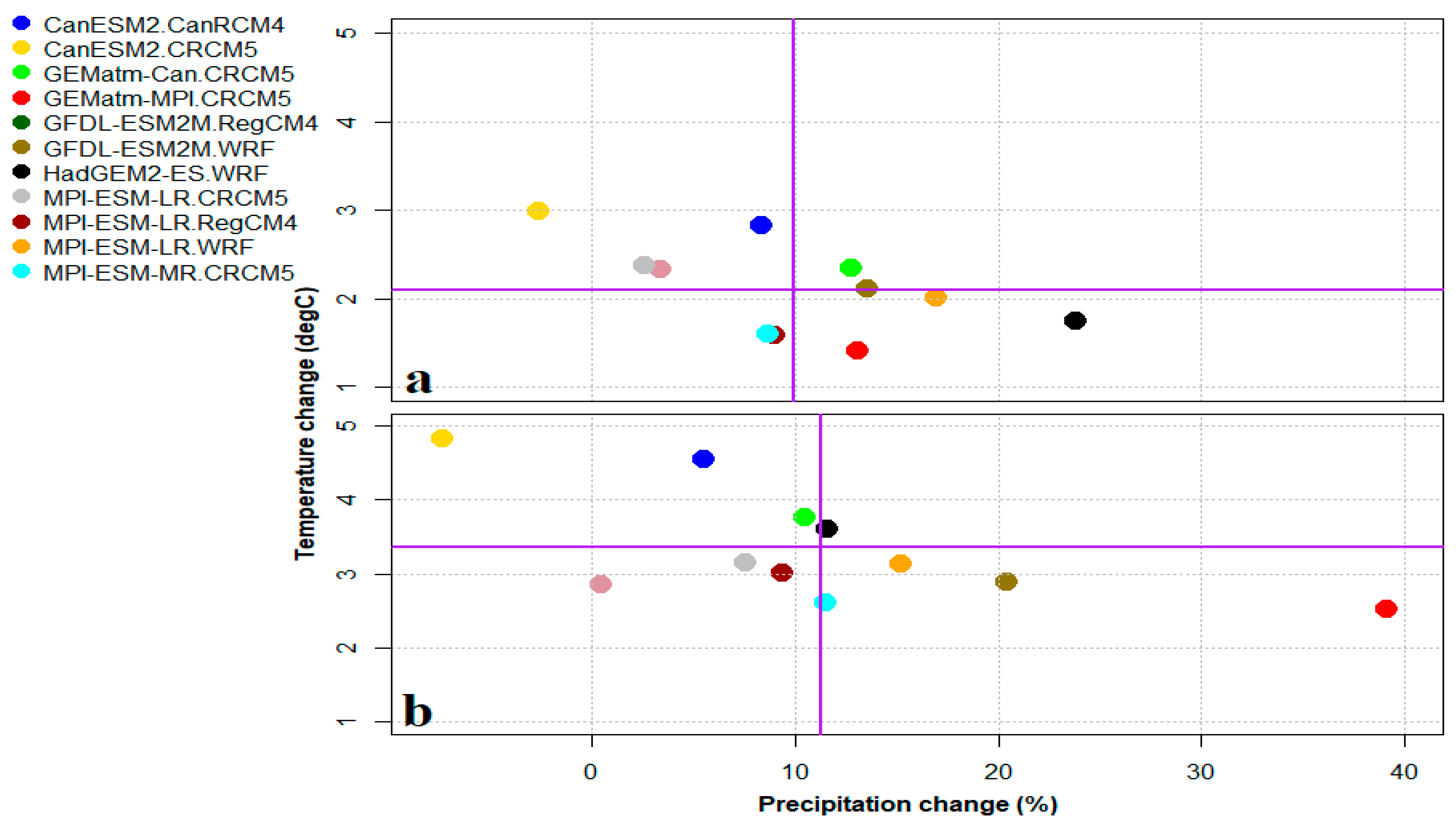
Figure 3 is scatter plots of projected mean precipitation change versus temperature between the future and historical periods. The annual changes in precipitation are positive for all RCMs except for CanESM2.CRCM5, while changes in mean annual temperature are positive for all RCM. Among the models, CanESM2.CRCM5 shows driest conditions for both periods whereas HadGEM2-ES.WRF and GEMatm-MPI.CRCM5 have the wettest conditions for the near future and distant future, respectively.
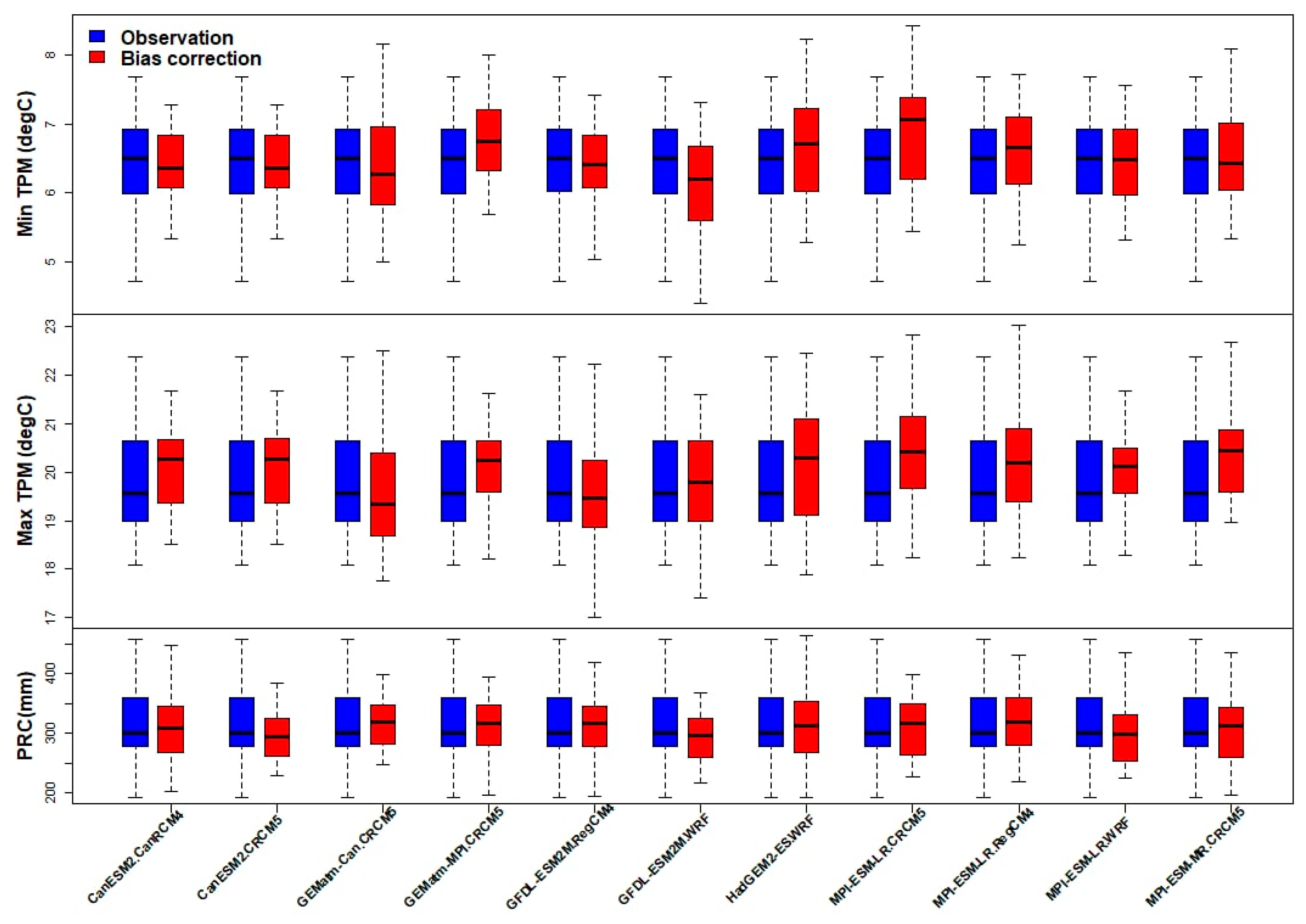
Multivariate Bias Correction with N-dimensional probability (MBCn) were tested using historical climate model data by the climate modeling centers that submitted their results to CORDEX. Figure 4 shows box whisker plot of annual mean values for minimum temperature, maximum temperature, and precipitation with respect to observation data and the 11 RCM models during the baseline period. The figure demonstrates that the differences between observations and bias corrected values are not significant for most of the 11 RCMs.
Figure 5 illustrates the temporal evolution of annual mean temperature, precipitation, solar radiation, and humidity for historical and projected periods. The ensemble median precipitation was 307 mm in the historical period, which increased 344 mm in the projections. Ensemble median minimum and maximum temperature were 6.7 °C and 20.1 °C in the historical period, respectively, while 9 °C and 22.6 °C in the projections, that is, increased by 2.2 and 2.5 °C in the future. Humidity ensemble results indicate that the historical value was 57.8% and it decreased 56% by the end of the century. The solar radiation ensemble mean has no significant changes between historical and projected periods.
3.3. Impact of Climate Change on a Drought Index
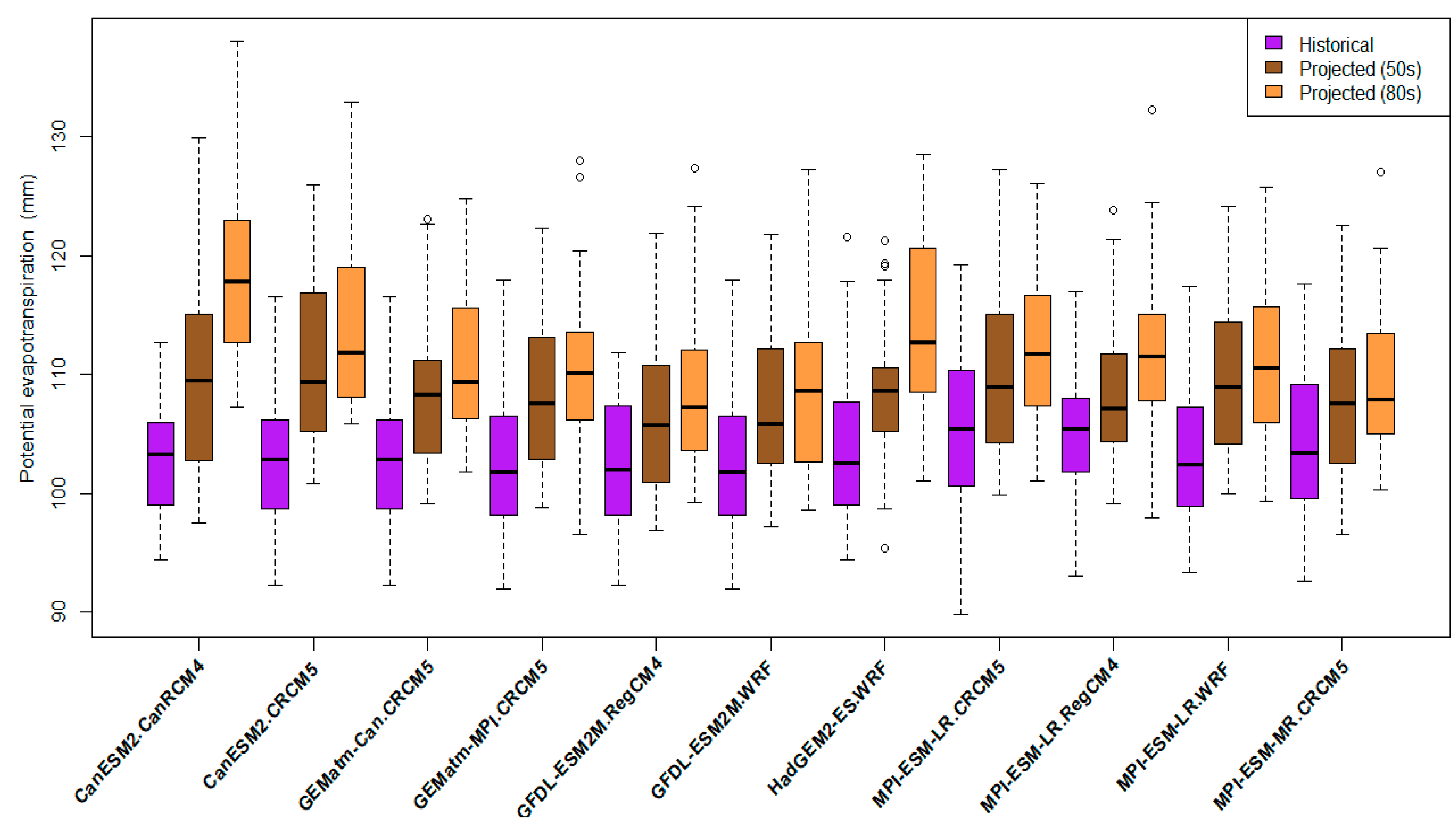
Figure 6 is a box plot of potential evapotranspiration (PET) derived from the 11 RCMs using the Penman–Monteith algorithm, for the three periods of historical (1975–2004), mid-century (2021–2050), and late century (2051–2080). Most of the climate model simulations have a similar pattern and trend, from historical to future. During the historical period, PET mean ranges from 89–121 mm, while it increased 95–130 mm in the middle period and 96–138 mm in the late period. The highest PET values in the projected period were found in ESM2.CRCM5 for the late century by 138 mm. The multi-RCM average warm season PET was projected to increase by 5.8% by mid-century and 14.5% in the late century relative to the historical period. DeJong et al. [42] reported an increase of 5.5–12% for the mid-century and 15–32% for the late century based on GCM output for Regina, reflecting the increases in mean annual temperature. Averaged between all 11 models, PET is expected to increase at a higher rate than precipitation for the period 2051–2080, while the amount of PET is less than precipitation for the middle period. Therefore, drier conditions can be expected at the end of the century in the region.
Different RCMs were used because we did not expect consistency among the RCMs. Therefore, we give results for multi-model mean values, but also show the range of future projections from 11 RCMs. Selecting RCMs that have good consistency with the observed weather parameters would be a good approach if the climate model data were not bias-corrected. The bias correction was done by the climate modeling centers that submit their experimental results to CORDEX. Given that this correction was conducted, we believe that the outputs of the model are quite reliable.
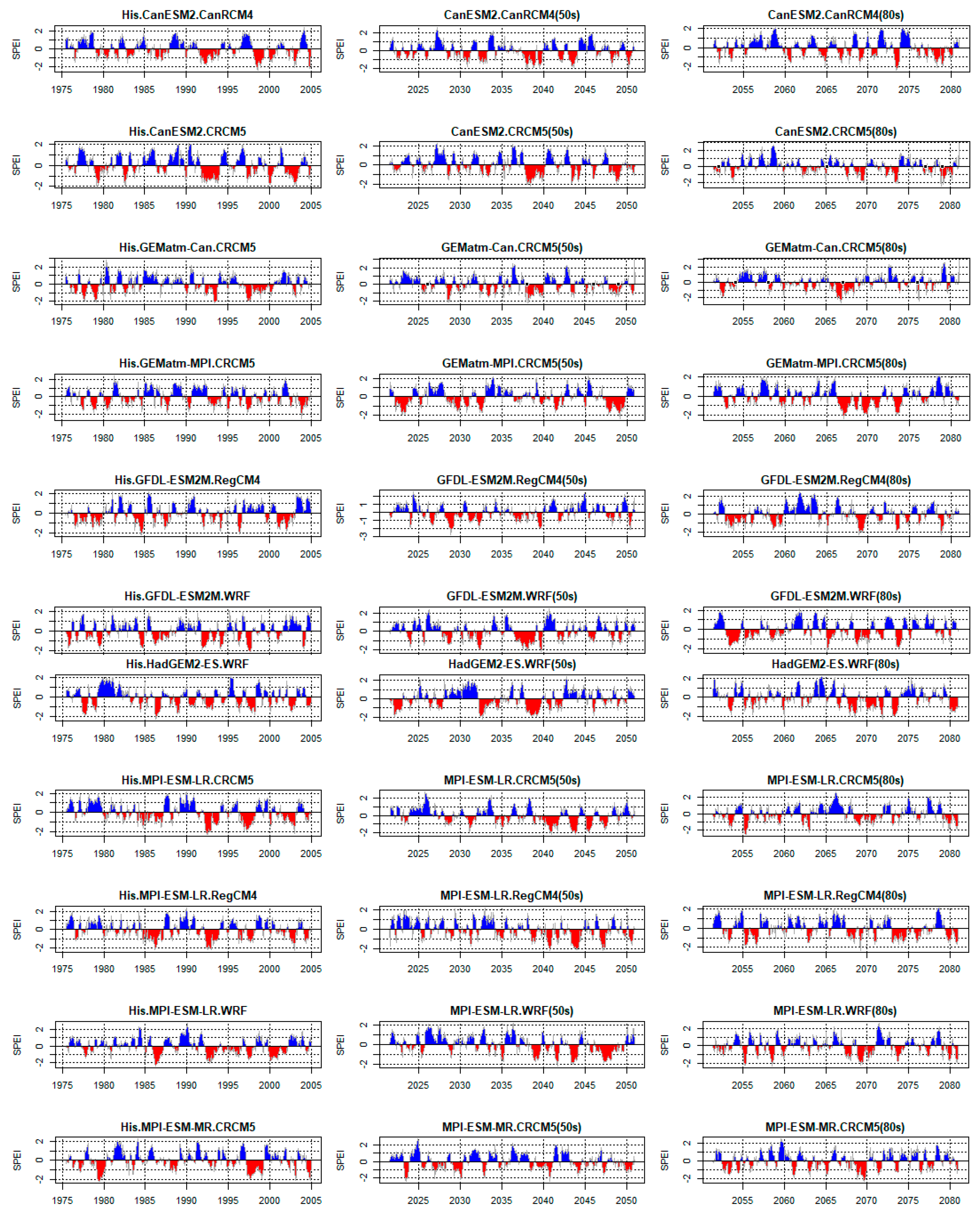
To assess drought, the Standardized Precipitation Evapotranspiration Index (SPEI) was calculated using the RCM data. Figure 7 gives the multi-model SPEI for a six-month interval computed using both historical data from 1975 to 2005 and simulated climate data according to the 11 RCM models from 2021 to 2080. Periods of extreme drought (SPEI < −2.5) is evident in all the time series. The results show more drought in the middle and end of century with monthly regional-averaged SPEI approximating less than −1.5. GFDL-ESM2M.RegCM4 (2028–2029) in the mid-century and CanESM2.CRCM5 (2078–2079) at the end of the century show extreme drought with a SPEI less than −2.5. Likewise, a frequency of two extreme drought events (SPEI < −2.0) in the historical period increases to four and five events in the middle and end of century, respectively. CanESM2.CRCM5 has the most frequent extreme drought event (seven) in the end century among all RCMs. Drought of longer duration is more common in projected climate compared with historical; the longest drought events (with SPEI < −1.0) are from GFDL-ESM2M.WRF. These results are consistent with that of Debike et al. [43], who showed an increase in severity of summer drought of up to 20% and 40% in the middle and late century, respectively, in Saskatchewan. The drought risk (increased drought severity and duration) will increase by the end of the century under the effect of rising temperature and evapotranspiration.
3.4. Impact of Climate Change on Soil Water Content
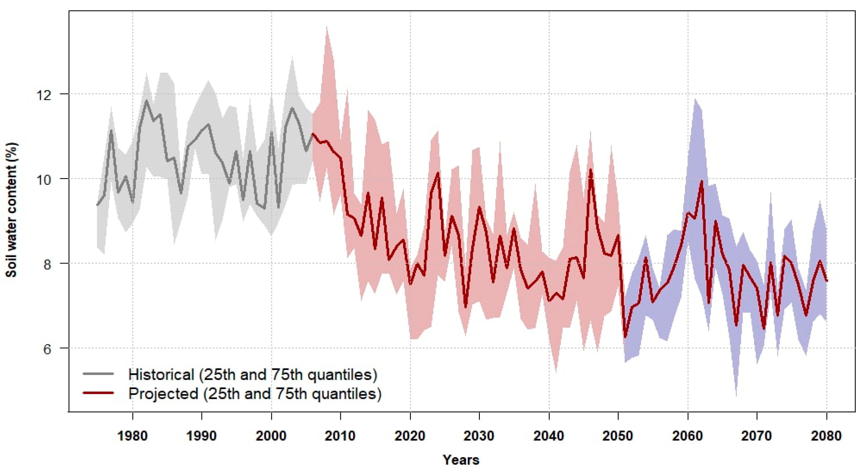
Figure 8 illustrates the temporal evolution of warm season SWC mean over the historical and projected periods. The ensemble median SWC was 11.2% in the historical period while it decreased to 8.4% and 7.9% in the middle and end centuries, respectively.
Figure 9 is box plots of the SWC simulated by the SWAT model for three periods of historical, middle, and end of century from the 11 RCMs. SWC has a similar pattern and trend among the models from historical to future. During the historical period, SWC median ranged from 8.5–11.5%, while it decreased 6.5–9.5% in the middle period and 5–8.9% in the end period. The highest and lowest SWC values in the projected periods were found in GEMatm-MPI.CRCM5 (18.7%) and CanESM2.CRCM5 (2.6%) in the second period.
Figure 10 shows the spatial pattern of warm season SWC per period for the 11 RCMs. The maps show similar distributions from historical to projected for all models. Generally, low SWC appears in the southwest to the west of the region, whereas high SWC is observed in the eastern part. Among all RCMs, GEMatm-MPI.CRCM5 in the historical period and CanESM2.CRCM5 in the last period shows the wettest and driest conditions across the region, respectively. There are obvious changing trends in most parts of the region from historical to projected revealed particularly by the map of GEMatm-Can.CRCM5.
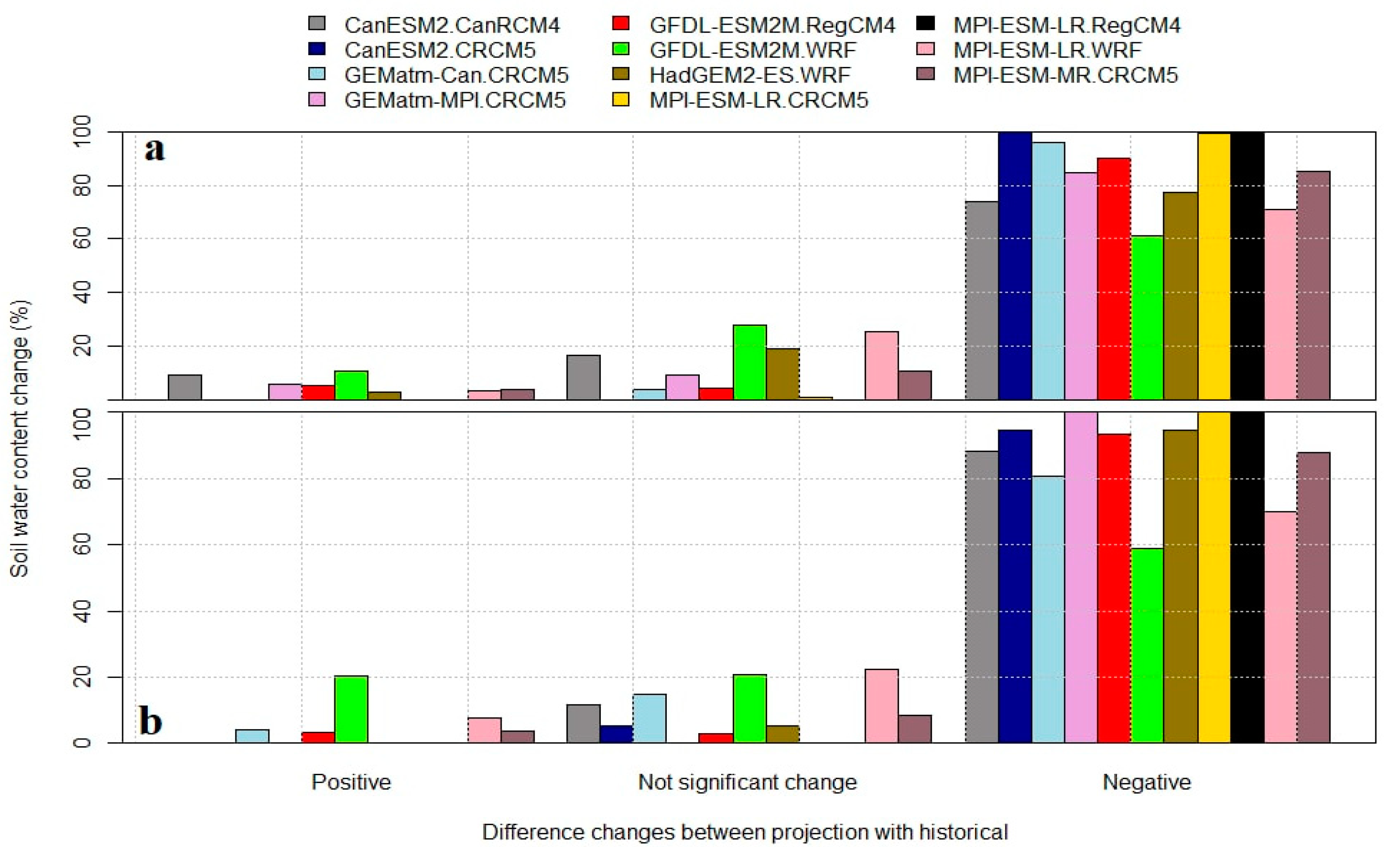
Figure 11 gives the spatial change in SWC in terms of the number of pixels in three categories: improved soil water content (positive), a loss of soil water content (negative), and no significant change. Among all models, only 5% of the region gains SWC, 27% has no significant change, and 68% of the region has a loss of SWC.
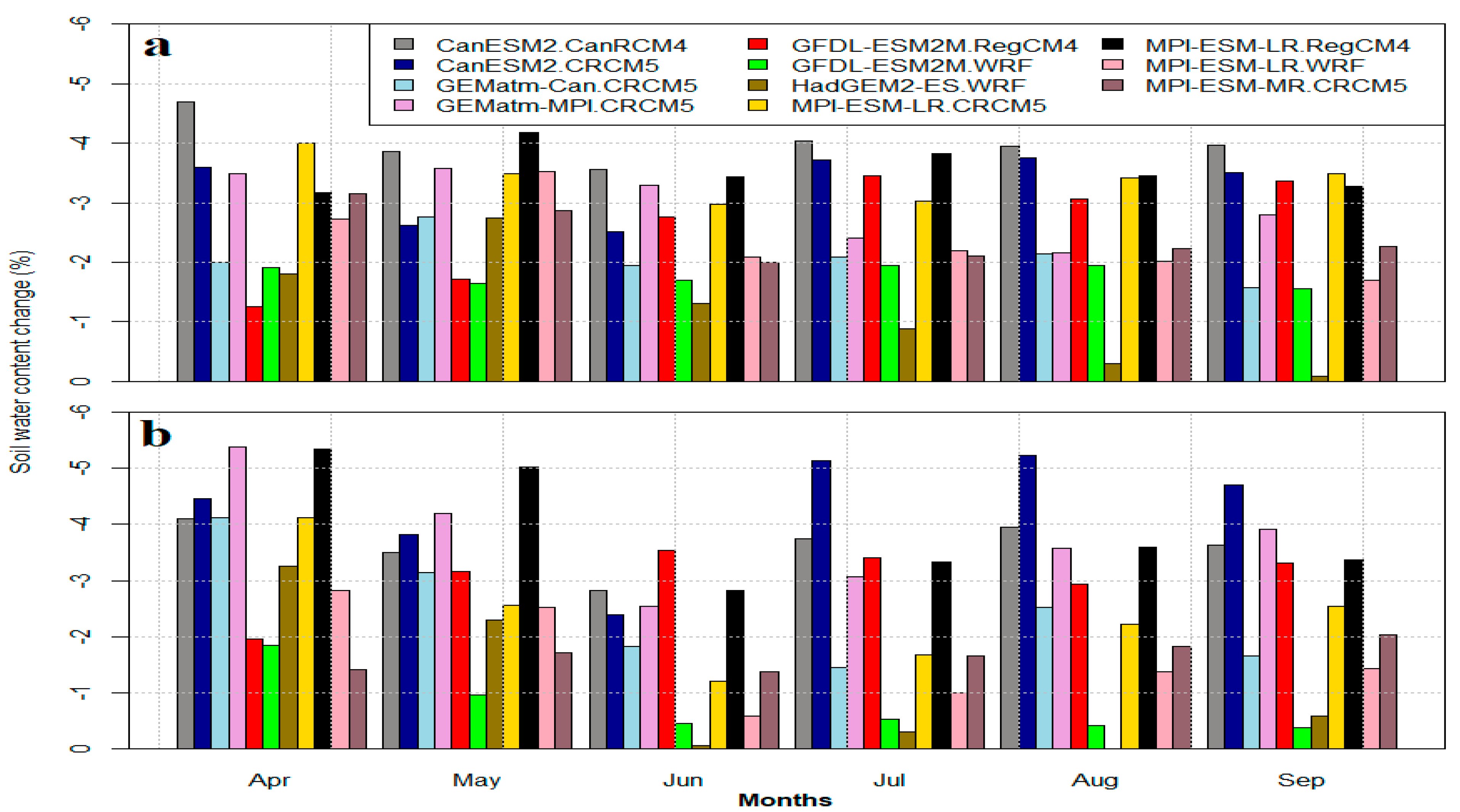
Figure 12 shows projected monthly changes in SWC from the historical to future periods. Results indicate that May loses the most SWC in the first period by 3% (average of all RCMs) while this value is unchanged for the second period. In the second period, maximum loss of SWC shifts from May to April when it is 3.6% (average of all RCMs). CanESM2.RCM4 in April has the highest change value (4.7%) in the middle period and CanESM2.CRCM5 in April has the highest change value (5.4%) in the late period. Soil moisture derived from snowmelt and precipitation in April to May, plus accumulations from the preceding autumn, are critical for water availability to crops during the subsequent growing season. Qian et al. [44] and Chipanshi et al. [45] confirm that climate change in Canada has a negative effect on soil moisture during the growing season, particularly in April.
Eleven different projections of SWC strongly suggest an overall future trend of drier conditions in the area as indicated when the projected changes in temperature and precipitation were combined into the SPEI indicator of drought stress. Average precipitation in southern Saskatchewan will likely increase; however, an increase in precipitation will not necessarily lead to wetter soil and surface conditions given increasing temperature and in turn rising evapotranspiration neutralizing the effect of precipitation. Increased warm season evapotranspiration will lead to a reduction in SWC levels. These findings agree with the observations of Diro and Sushama [46], who reported a decrease of 10% to 20% for the late-century period using CRCM5 in southern Saskatchewan. Kienzle et al. [47] found an increase of 0.5% in the 2020s, 1.4% by the 2050s, and 2.6% by the 2080s. They mentioned that earlier snowmelt could result in increased soil moisture earlier in the spring, and that soil moisture deficits can be expected in the summer when potential evaporation will be higher in the future. Pomeroy et al. [48] reported climate studies for southern Saskatchewan confirming that a doubling of atmospheric CO2 will result in an increased air temperature (up to 8 °C during winter), a decreased snowpack, an earlier snowmelt, and a drop in summer soil moisture. A review of the literature on SWC projections reveals that due to the frequency of drought predicted in the region, the southern part of the prairies could experience significant soil moisture deficits during the summer months by the end of this century.
4. Summary and Conclusions
The ArcSWAT model was employed for the calibration of SWC and the model performed well in simulating mean monthly streamflow the Qu’Appelle River basin with BIAS less than 10% and NSE and R higher than 0.8. Increased accuracy of the models was achieved by running them with daily weather and soil moisture data, along with satellite soil moisture (SMAP) data over a longer time. We employed multivariable calibration via evaluation of monthly streamflow along with daily SWC. This improved the reliability of parameters for simulating hydrology components in the Qu’Appelle River basin. We demonstrated that the calibrated model is applicable for estimating the impact of climate change on future SWC in southern Saskatchewan. According to the RCM model means, in the near future and distant future, mean temperature will increase 2.1 °C and 3.4 °C, and precipitation will increase 10% and 11.25%. We ran the calibrated SWAT model with climate forcing from the 11 RCMs. The average of all model runs showed decreased soil moisture, despite an increase in annual precipitation, so that the following relative changes in soil moisture can be expected in the region: a decrease of 3.6% in 2021–2050 and 4% in 2051–2070. The primary mechanisms of an increase in drought frequencies are increasing evaporation driven by rising temperatures and longer warm seasons, which neutralizes the effect of increased rainfall. We found that all 11 SWAT-RCM experiments exhibit similar SWC changes in the middle and late centuries, with the milder GEMatm-MPI RCM producing a slightly more significant increase. In contrast, CanESM2 exhibited more significant drought in the same period. The pattern of spatial SWC for the 11 RCMs is similar with the northwest and western parts of the region wetter than in the south and east. The spatially averaged soil moisture had no obvious change within the historical and projected periods, while SWC values had a sharp decrease between the past and the future.
Soil moisture plays a vital role in dryland agriculture, which is reliant on rain and snowmelt in cold climates. Low SWC in the warm season is problematic for the production of dryland crops; these challenging conditions will intensify in the presence of climate change. Increasing extreme temperature and declining SWC can result in severe yield reduction with negative impact in the growing stage for local crops such as wheat and canola. This study improves our understanding of climate change effects on soil water content and can help support sustainable solutions related to food and water security under climate change in southern Saskatchewan.
Author Contributions
Data curation and analysis, M.Z.; supervision, S.A. and D.S.; writing—original draft, M.Z.; writing—review and editing, S.A. and D.S. All authors have read and agreed to the published version of the manuscript.
Funding
This research received no external funding.
Institutional Review Board Statement
Not applicable.
Informed Consent Statement
Not applicable.
Data Availability Statement
The authors can provide access to modeling data upon request.
Acknowledgments
The authors would like to thank the University of Regina for providing computational facilities and Natural Science and Engineering Research Council of Canada.
Conflicts of Interest
The authors declare there is no conflict of interest.
References
- Pomeroy, J.W.; Gray, D.M.; Brown, T.; Hedstrom, N.R.; Quinton, W.; Granger, R.J.; Carey, S. The cold regions hydrological model: A platform for basing process representation and model structure on physical evidence. Hydrol. Process. 2007, 21, 2650–2667. [Google Scholar] [CrossRef]
- Mamassis, N.; Panagoulia, D.; Novkovic, A. Sensitivity analysis of penman evaporation method. Glob. Nest J. 2014, 16, 628–639. [Google Scholar]
- Akhter, A.; Azam, S. Flood-drought hazard assessment for a flat clayey deposit in the Canadian Prairies. J. Environ. Inform. Lett. 2019, 1, 8–19. [Google Scholar] [CrossRef]
- Barnett, T.; Adam, J.; Lettenmaier, D.P. Potential impacts of a warming climate on water availability in snow-dominated regions. Nature 2005, 438, 303–309. [Google Scholar] [CrossRef]
- Feng, H.; Liu, Y. Combined effects of precipitation and air temperature on soil moisture in different land covers in a humid basin. J. Hydrol. 2015, 531, 1129–1140. [Google Scholar] [CrossRef]
- Bouslihim, Y.; Kacimi, I.; Brirhet, H.; Khatati, M.; Rochdi, A.; Pazza, N.E.A.; Miftah, A.; Yaslo, Z. Hydrologic modeling using SWAT and GIS, application to subwatershed Bab-Merzouka (Sebou, Morocco). J. Geogr. Inf. Syst. 2016, 8, 20–27. [Google Scholar] [CrossRef] [Green Version]
- Sauchyn, D.; Barrow, E.; Fang, X.; Henderson, N.; Johnston, M.; Pomeroy, J.; Thorpe, J.; Wheaton, E.; Williams, B. Saskatchewan’s Natural Capital in a Changing Climate: An Assessment of Impacts and Adaptation; Report to Saskatchewan Ministry of Environment; Prairie Adaptation Research Collaborative: Regina, SK, Canada, 2009; 162p. [Google Scholar]
- Morales-Marin, L.; Wheater, H.; Lindenschmidt, K.E. Potential Changes of Annual-Averaged Nutrient Export in the South Saskatchewan River Basin under Climate and Land-Use Change Scenarios. Water 2018, 10, 1438. [Google Scholar] [CrossRef] [Green Version]
- Dibike, Y.; Muhammad, A.; Shrestha, R.; Spence, C.; Bonsal, B.; de Rham, L.; Rowley, J.; Evenson, G.; Stadnyk, T. Application of dynamic contributing area for modelling the hydrologic response of the Assiniboine River basin to a changing climate. J. Great Lakes Res. 2021, 47, 663–676. [Google Scholar] [CrossRef]
- Herceg, A.; Kalicz, P.; Gribovszki, Z. The impact of land use on future water balance—A simple approach for analysing climate change effects. Forest 2021, 14, 175–185. [Google Scholar] [CrossRef]
- Keshta, N.; Elshorbagy, A.; Carey, S. Impacts of climate change on soil moisture and evapotranspiration in reconstructed watersheds in northern Alberta, Canada. Hydrol Process. 2012, 26, 1321–1331. [Google Scholar] [CrossRef]
- Chiew, F.; Whetton, P.H.; McMahon, T.A.; Pittock, A.B. Simulation of the impacts of climate change on runoff and soil moisture in Australian catchments. J. Hydrol. 1995, 167, 121–147. [Google Scholar] [CrossRef]
- Berg, A.; Sheffield, J. Climate Change and Drought: The Soil Moisture Perspective. Curr. Clim. Change Rep. 2018, 4, 180–191. [Google Scholar] [CrossRef]
- Bradford, J.B.; Schlaepfer, D.R.; Lauenroth, W.K.; Palmquist, K.A.; Chambers, J.C.; Maestas, J.D.; Campbell, S.B. Climate-Driven Shifts in Soil Temperature and Moisture Regimes Suggest Opportunities to Enhance Assessments of Dryland Resilience and Resistance. Front. Ecol. Evol. 2019, 7, 358. [Google Scholar] [CrossRef] [Green Version]
- Hosten, A.; Vetter, T.; Vohland, K.; Krysanova, V. Impact of climate change on soil moisture dynamics in Brandenburg with a focus on nature conservation areas. Ecol. Model. 2009, 220, 2076–2087. [Google Scholar] [CrossRef]
- Kellomäki, S.; Maajärvi, M.; Strandman, H.; Kilpeläinen, A.; Peltola, H. Model computations on the climate change effects on snow cover, soil moisture and soil frost in the boreal conditions over Finland. Silva Fenn. 2010, 44, 213–233. [Google Scholar] [CrossRef] [Green Version]
- Narasimhan, B.; Srinivasan, R. Development and evaluation of Soil Moisture Deficit Index (SMDI) and Evapotranspiration Deficit Index (ETDI) for agricultural drought monitoring. Agric. For. Meteorol. 2005, 133, 69–88. [Google Scholar] [CrossRef]
- Wang, X.; Xie, H.; Guan, H.; Zhou, X. Different responses of MODIS-derived NDVI to root-zone soil moisture in semi-arid and humid regions. J. Hydrol. 2011, 340, 12–24. [Google Scholar] [CrossRef]
- Park, J.Y.; Ahn, S.R.; Hwang, S.J.; Jang, C.H.; Park, G.A.; Kim, S.J. Evaluation of MODIS NDVI and LST for indicating soil moisture of forest areas based on SWAT modeling. Int. Soc. Pad. Water Environ. Eng. 2014, 121, 77–88. [Google Scholar] [CrossRef]
- Havrylenko, S.B.; Bodoque, J.M.; Srinivasan, R.; Zucarelli, G.V.; Mercuri, P. Assessment of the soil wa-ter content in the Pampas region using SWAT. Catena 2016, 137, 298–309. [Google Scholar] [CrossRef]
- Nilawar, A.P.; Calderella, C.P.; Lakhankar, T.Y. Satellite soil moisture validation using hydrological SWAT model: A case study of Puerto Rico, USA. Hydrology 2017, 4, 45. [Google Scholar] [CrossRef] [Green Version]
- Rajib, A.; Merwade, V.; Kim, I.L.; Zhao, L.; Song, C.; Zhe, S. SWATShare—A web platform for collabo-rative research and education through online sharing, simulation and visualization of SWAT models. Environ. Model. Softw. 2016, 75, 498–512. [Google Scholar] [CrossRef] [Green Version]
- Azimi, S.; Dariane, A.; Modanesi, S.; Bauer-Marschallinger, B.; Bindlish, R.; Wagner, W.; Massari, C. Assimilation of Sentinel 1 and SMAP—Based satellite soil moisture retrievals into SWAT hydrological model: The impact of satellite revisit time and product spatial resolution on flood simulations in small basins. J. Hydrol. 2020, 581, 124367. [Google Scholar] [CrossRef] [PubMed]
- Zare, M.; Azam, S.; Sauchyn, D. Evaluation of Soil Water Content Using SWAT for Southern Saskatchewan, Canada. Water 2022, 14, 249. [Google Scholar] [CrossRef]
- Abbaspour, K.C. SWAT-CUP: SWAT Calibration and Uncertainty Programs—A User Manual; Open File Rep.; Eawag, Swiss Federal Institute of Aquatic Science and Technology: Dübendorf, Switzerland, 2015; 100p. [Google Scholar]
- Arnold, J.G.; Moriasi, D.N.; Gassman, P.W.; Abbaspour, K.C.; White, M.J.; Srinivasan, R.; Santhi, C.; Harmel, R.D.; Van Griensven, A.; Van Liew, M.W.; et al. SWAT: Model use, calibration, and validation. Trans. ASABE 2012, 55, 1491–1508. [Google Scholar] [CrossRef]
- Abbaspour, K.C.; Yang, J.; Maximov, I.; Siber, R.; Bogner, K.; Mieleitner, J.; Zobrist, J.; Srinivasan, R. Modelling hydrology and water quality in the pre-alpine/alpine Thur watershed using SWAT. J. Hydrol. 2007, 333, 413–430. [Google Scholar] [CrossRef]
- Mearns, L.; McGinnis, S.; Korytina, D.; Arritt, R. The NA-CORDEX Dataset, Version 1.0. NCAR Climate Data Gateway, Boulder CO. 2017. Available online: https://doi.org/10.5065/D6SJ1JCH (accessed on 16 May 2017).
- van Griensven, A.; Meixner, T.; Grunwald, S.; Bishop, T.; Di Luzio, M.; Srinivasan, R. A global sensitivity analysis method for the parameters of multi-variable watershed models. J. Hydrol. 2006, 324, 10–23. [Google Scholar] [CrossRef]
- Moriasi, D.N.; Arnold, J.G.; Van Liew, M.W.; Binger, R.L.; Harmel, R.D.; Veith, T. Model evaluation guidelines for systematic quantification of accuracy in watershed simulations. Trans. ASABE 2007, 50, 885–900. [Google Scholar] [CrossRef]
- Gyamfi, C.; Ndambuki, J.M.; Salim, R.W. Application of SWAT model to the Olifants Basin: Calibration, validation and uncertainty analysis. J. Water Resour. Prot. 2016, 8, 397–410. [Google Scholar] [CrossRef] [Green Version]
- Khalid, K.; Rahman, A. Sensitivity Analysis in Watershed Model Using SUFI-2 Algorithm. Procedia Eng. 2016, 162, 441–447. [Google Scholar] [CrossRef] [Green Version]
- Thavhana, M.P.; Savage, M.J.; Moeletsi, M.E. SWAT model uncertainty analysis, calibration and validation for runoff simulation in the Luvuvhu River catchment, South Africa. Phys. Chem. Earth 2018, 105, 115–124. [Google Scholar] [CrossRef]
- Van Liew, M.W.; Garbrecht, J. Hydrologic Simulation of the Little Washita River Experimental Watershed Using SWAT. J. Am. Water Resour. Assoc. 2003, 39, 413–426. [Google Scholar] [CrossRef]
- Chapuis, R.P. Predicting the saturated hydraulic conductivity of soils: A review. Bull. Eng. Geol. Environ. 2012, 71, 401–434. [Google Scholar] [CrossRef]
- Opere, A.O.; Okello, B.N. Hydrologic analysis for river Nyando using SWAT. Hydrol. Earth Syst. Sci. 2011, 8, 1765–1797. [Google Scholar]
- Rossi, C.G.; Srinivasan, R.; Jirayoot, K.; Le Duc, T.; Souvannabouth, P.; Binh, N. Hydrologic evaluation of the Lower Mekong River Basin with the soil and water assessment tool model. Int. Agric. Eng. J. 2009, 18, 1–13. [Google Scholar]
- Mengistu, D.T.; Sorteberg, A. Sensitivity of SWAT simulated streamflow to climatic changes within the Eastern Nile River basin. Hydrol. Earth Syst. Sci. 2012, 16, 391–407. [Google Scholar] [CrossRef] [Green Version]
- Tanzeeba, S.; Gan, T.Y. Potential impact of climate change on the water availability of South Saskatchewan River Basin. Clim. Change 2012, 112, 355–386. [Google Scholar] [CrossRef]
- He, Y.; Wang, H.; Qian, B.; McConkey, B.; DePauw, R. How early can the seeding dates of spring wheat be under current and future climate in Saskatchewan, Canada? PLoS ONE 2012, 7, e45153. [Google Scholar] [CrossRef] [Green Version]
- Islam, Z.; Gan, T.Y. Potential combined hydrologic impacts of climate change and El Niño Southern Oscillation to South Saskatchewan River Basin. J. Hydrol. 2015, 523, 34–48. [Google Scholar] [CrossRef]
- DeJong, J.T.; Mortensen, B.M.; Martinez, B.C.; Nelson, D.C. Bio-mediated soil improvement. Ecol. Eng. 2010, 36, 197–210. [Google Scholar] [CrossRef]
- Dibike, Y.; Prowse, T.; Bonsal, B.; Oneil, H. Implications of future climate on water availability in the western Canadian river basins. Int. J. Climatol. 2017, 37, 3247–3263. [Google Scholar] [CrossRef]
- Qian, B.; De Jong, R.; Gameda, S.; Huffman, T.; Neilsen, D.; Desjardins, R.; Wang, H.; McConkey, B. Impact of climate change scenarios on Canadian agroclimatic indices. Can. J. Soil Sci. 2013, 93, 243–259. [Google Scholar] [CrossRef]
- Chipanshi, A.; Berry, M.; Zhang, Y.; Qian, B. Agroclimatic indices across the Canadian Prairies under a changing climate and their implications for agriculture. Int. J. Climatol. 2021, 32, 2351–2367. [Google Scholar] [CrossRef]
- Diro, G.T.; Sushama, L. The Role of Soil Moisture–Atmosphere Interaction on Future Hot Spells over North America as Simulated by the Canadian Regional Climate Model (CRCM5). Am. Meteorol. Soc. 2017, 30, 5041–5058. [Google Scholar] [CrossRef]
- Kienzle, S.W.; Nemeth, M.W.; Byrne, J.M.; MacDonald, R.J. Simulating the hydrological impacts of climate change in the upper North Saskatchewan River basin, Alberta, Canada. J. Hydrol. 2012, 412, 76–89. [Google Scholar] [CrossRef]
- Pomeroy, J.; Fang, X.; Williams, B. Impacts of Climate Change on Saskatchewan’s Water Resources; Centre for Hydrology, University of Saskatchewan: Saskatoon, SK, Canada, 2009. [Google Scholar]
Figure 1.
Map of the study region (modified after [24]).
Figure 1.
Map of the study region (modified after [24]).

Figure 2.
Monthly simulated and observed flows during the calibration period (1995–2004) and validation period (2005–2010).
Figure 2.
Monthly simulated and observed flows during the calibration period (1995–2004) and validation period (2005–2010).

Figure 3.
Scatter plots of annual changes in mean temperature and total precipitation in the region for (a) 2050s and (b) 2080s. Purple lines give average of temperature and precipitation for all RCMs.
Figure 3.
Scatter plots of annual changes in mean temperature and total precipitation in the region for (a) 2050s and (b) 2080s. Purple lines give average of temperature and precipitation for all RCMs.

Figure 4.
Box-whisker plots of the precipitation and minimum and maximum temperature derived from the observed and RCMs data.
Figure 4.
Box-whisker plots of the precipitation and minimum and maximum temperature derived from the observed and RCMs data.

Figure 5.
Weather parameters time series for the reference period 1976–2005 mean and RCP8.5 projections from 2005–2080. Solid lines indicate the ensemble medians and the shadings show the interquartile ensemble spread (25th and 75th quantiles).
Figure 5.
Weather parameters time series for the reference period 1976–2005 mean and RCP8.5 projections from 2005–2080. Solid lines indicate the ensemble medians and the shadings show the interquartile ensemble spread (25th and 75th quantiles).

Figure 6.
Temporally averaged PET in historical and projected changes.

Figure 7.
Temporal variation of SPEI at 6-month scale under historical and projected changes.

Figure 8.
Soil water content relative to the reference period 1976–2005 mean for RCP8.5 over the region. Solid lines show the ensemble medians and the shadings show the interquartile ensemble spread (25th and 75th quantiles).
Figure 8.
Soil water content relative to the reference period 1976–2005 mean for RCP8.5 over the region. Solid lines show the ensemble medians and the shadings show the interquartile ensemble spread (25th and 75th quantiles).

Figure 9.
Box plots of the range of SWC under historical and projected changes.

Figure 10.
Annual spatial SWC in the historical period, and middle and late century.

Figure 11.
Spatial SWC change between RCM models in (a) near future and (b) distant future.

Figure 12.
Monthly difference changes between (a) near future with historical and (b) distant future with historical.
Figure 12.
Monthly difference changes between (a) near future with historical and (b) distant future with historical.


Table 1.
Summary of climate station.
| Station Name | Latitude (N) | Longitude (W) | Elevation (m) | Start Date | End Date | Years |
|---|---|---|---|---|---|---|
| Broadview | 50°22′05.000″ | 102°34′15.000″ | 599.80 | 1985 | 2020 | 36 |
| Buffalo pound lake | 50°33′00.000″ | 105°23′00.000″ | 588.00 | 1985 | 2020 | 36 |
| Qu’Appelle | 50°34′00.000″ | 103°59′00.000″ | 662.90 | 1985 | 2020 | 36 |
| Kelliher | 51°15′26.700″ | 103°45′10.900″ | 675.60 | 1985 | 2020 | 36 |
| Moose Jaw | 50°19′54.050″ | 105°32′15.030″ | 577.00 | 1998 | 2020 | 23 |
| Lipton 2 | 51°09′08.008″ | 103°53′22.001″ | 640.00 | 1985 | 2020 | 36 |
| Yellow grass | 49°49′00.000″ | 104°11′00.000″ | 579.70 | 1985 | 2018 | 34 |
| Langenburg | 50°54′00.000″ | 101°43′00.000″ | 516.60 | 1985 | 2020 | 36 |
| Leroy | 52°00′00.000″ | 104°38′00.000″ | 535.40 | 1985 | 2020 | 36 |
| Rock point | 51°09′14.007″ | 107°15′48.004″ | 725.10 | 1985 | 2020 | 36 |
| Elbow | 51°08′00.000″ | 106°35′00.000″ | 595.00 | 1985 | 2020 | 36 |
| Last mountain | 51°25′00.000″ | 105°15′00.000″ | 497.00 | 1985 | 2020 | 36 |
| Watrous | 51°40′00.000″ | 105°24′00.000″ | 525.60 | 1985 | 2020 | 36 |
| Indian head | 50°33′00.000″ | 103°39′00.000″ | 579.10 | 1985 | 2020 | 36 |
| Lucky lake | 50°57′00.000″ | 107°09′00.000″ | 664.70 | 1985 | 2020 | 36 |
Table 2.
Summary of NA-CORDEX simulations.
| Simulation Name | GCM Derived | RCM Model Name | Institute |
|---|---|---|---|
| CanESM2.CanRCM4 | CanESM2 | Canadian Regional Climate Model version 4 | Canadian Centre for Climate Modelling and Analysis (CCCma) |
| CanESM2.CRCM5 | CanESM2 | Canadian Regional Climate Model (CRCM) version 5 | Université du Québec à Montréal (UQAM) |
| GEMatm-Can.CRCM5 | GEMatm | Canadian Regional Climate Model (CRCM) version 5 | Université du Québec à Montréal (UQAM) |
| GEMatm-MPI.CRCM5 | GEMatm | Canadian Regional Climate Model (CRCM) version 5 | Université du Québec à Montréal (UQAM) |
| GFDL-ESM2M.RegCM4 | GFDL-ESM2 | Regional Climate Model version 4 | Iowa State University and the National Center for Atmospheric Research (NCAR) |
| GFDL-ESM2M.WRF | GFDL-ESM2 | Weather Research and Forecasting model | University of Arizona and NCAR |
| HadGEM2-ES.WRF | HadGEM2-ES | Weather Research and Forecasting model | University of Arizona and NCAR |
| MPI-ESM-LR.CRCM5 | MPI-ESM-LR | Canadian Regional Climate Model (CRCM) version 5 | Université du Québec à Montréal (UQAM) |
| MPI-ESM-LR.RegCM4 | MPI-ESM-LR | Regional Climate Model version 4 | Iowa State University and the National Center for Atmospheric Research (NCAR) |
| MPI-ESM-LR.WRF | MPI-ESM-LR | Weather Research and Forecasting model | University of Arizona and NCAR |
| MPI-ESM-MR.CRCM5 | MPI-ESM-MR | Canadian Regional Climate Model (CRCM) version 5 | Université du Québec à Montréal (UQAM) |
Table 3.
Parameters used for calibration with optimum values.
| Parameter | Description | Type | Initial Range | Optimal Value | p-Value | t-State | Rank |
|---|---|---|---|---|---|---|---|
| ALPHA_BF | Base flow alpha factor | v | 0.0–1.0 | 0.1–0.241 | 0.000 | −36.26 | 1 |
| GW_REVAP | Ground water re-evaporation coefficient | v | −0.2–0.2 | 0.1–0.17 | 0.000 | 16.89 | 2 |
| CH_K2 | Effective hydraulic conductivity in main channel alluvium (mm/h) | v | 0.0–500 | 154–642 | 0.001 | 14.73 | 3 |
| CN2 | Curve number at moisture condition II | r | −0.2–0.2 | −0.13–0.038 | 0.008 | 13.21 | 4 |
| GWQMN | Threshold depth of water in the shallow aquifer required for return flow (mm) | r | 0.0–0.2 | 0.64–1.94 | 0.074 | 10.9 | 5 |
| SOL_ALB | Moist soil albedo | r | 0–0.25 | 0.08–0.139 | 0.08 | −10.7 | 6 |
| ESCO | Soil evaporation compensation factor | v | 0.0–1.0 | 0.241–0.832 | 0.354 | 9.26 | 7 |
| CH_N2 | Manning’s ”n” value for the channel | v | 0.0–0.3 | 0.09–0.272 | 0.382 | −8.74 | 8 |
| GW_DELAY | Groundwater delay (days) | v | 0–500 | 181–272 | 0.533 | −0.623 | 9 |
| SOL_BD | Saturated hydraulic conductivity of first layer | r | −0.1–1.0 | −0.005–0.183 | 0.551 | 0.596 | 10 |
| SURLAG | Surface runoff lag coefficient (day) | v | 0.0–24 | 2.68–23.04 | 0.787 | 0.272 | 11 |
| SOL_AWC | Soil water available capacity | r | −0.1–1.0 | −0.061–0.357 | 0.796 | 0.257 | 12 |
| SOL_K | Saturated hydraulic conductivity (mm/h) | r | −0.1–1.0 | −0.011–0.027 | 0.803 | −0.248 | 13 |
| SOL_Z | Depth from the soil surface to layer bottom | r | −0.1–1.0 | −0.03–0.021 | 0.842 | −0.198 | 14 |
Table 4.
Daily calibration of SWAT model with field measurement data and SMAP.
| Data | RMSE | Bias | R | p-Value | N | |
|---|---|---|---|---|---|---|
| Measurement | SWAT | 0.046 | 0.012 | 0.000 | 703 | |
| SMAP | 0.052 | −0.035 | 0.000 | 703 | ||
| SWAT | SMAP | 0.106 | −0.096 | 0.000 | 703 | |
Table 5.
Annual changes relative to baseline period in weather parameters under RCP8.5.
| RCM | T Mean (°C) | Precipitation (%) | Solar Radiation (%) | Humidity (%) | ||||
|---|---|---|---|---|---|---|---|---|
| 50 s | 80 s | 50 s | 80 s | 50 s | 80 s | 50 s | 80 s | |
| CanESM2.CanRCM4 | 2.82 | 4.54 | 8.31 | 5.53 | 2.67 | −0.86 | −2.79 | −1.54 |
| CanESM2.CRCM5 | 3.00 | 4.83 | −2.65 | −7.4 | 0.48 | −2.42 | −5.1 | −4.62 |
| GEMatm-Can.CRCM5 | 2.34 | 3.75 | 12.77 | 10.5 | 1.34 | −2.67 | −0.42 | 1.79 |
| GEMatm-MPI.CRCM5 | 1.41 | 2.52 | 13.06 | 39.16 | −1.21 | −1.38 | −0.32 | 0.31 |
| GFDL-ESM2M.RegCM4 | 2.33 | 2.86 | 3.33 | 0.44 | 4.54 | −3.38 | −3.69 | −2.59 |
| GFDL-ESM2M.WRF | 2.11 | 2.88 | 13.56 | 20.41 | 3.22 | −4 | −0.99 | 2.33 |
| HadGEM2-ES.WRF | 1.75 | 3.6 | 23.87 | 11.57 | −0.43 | 0.07 | 1.79 | −1.33 |
| MPI-ESM-LR.CRCM5 | 2.37 | 3.15 | 2.61 | 7.51 | 1.23 | 1.23 | −6.24 | −2.06 |
| MPI-ESM-LR.RegCM4 | 1.58 | 3.02 | 9.01 | 9.34 | 0.41 | 1.05 | −3.84 | −3.18 |
| MPI-ESM-LR.WRF | 2.01 | 3.12 | 16.97 | 15.24 | 2.87 | −3.94 | −3.74 | 0.91 |
| MPI-ESM-MR.CRCM5 | 1.60 | 2.61 | 8.68 | 11.46 | −0.7 | −1.96 | −1.66 | −0.02 |
Publisher’s Note: MDPI stays neutral with regard to jurisdictional claims in published maps and institutional affiliations. |
© 2022 by the authors. Licensee MDPI, Basel, Switzerland. This article is an open access article distributed under the terms and conditions of the Creative Commons Attribution (CC BY) license (https://creativecommons.org/licenses/by/4.0/).
Share and Cite
MDPI and ACS Style
Zare, M.; Azam, S.; Sauchyn, D. Impact of Climate Change on Soil Water Content in Southern Saskatchewan, Canada. Water 2022, 14, 1920. https://doi.org/10.3390/w14121920
AMA Style
Zare M, Azam S, Sauchyn D. Impact of Climate Change on Soil Water Content in Southern Saskatchewan, Canada. Water. 2022; 14(12):1920. https://doi.org/10.3390/w14121920
Chicago/Turabian StyleZare, Mohammad, Shahid Azam, and David Sauchyn. 2022. "Impact of Climate Change on Soil Water Content in Southern Saskatchewan, Canada" Water 14, no. 12: 1920. https://doi.org/10.3390/w14121920
Note that from the first issue of 2016, this journal uses article numbers instead of page numbers. See further details here.