River–Groundwater Interaction and Recharge Effects on Microplastics Contamination of Groundwater in Confined Alluvial Aquifers

Abstract

Literature provides only a few examples of contamination of groundwater with microplastics, mainly investigated using a chemical approach. Little importance is given to the hydrogeological processes able to affect the contamination, such as river–groundwater interactions. This study was carried out with two aims. The first aim is the formulation of a method with a high result-to-cost ratio, based on the hydrogeological aspects of the investigated area. Microplastics were extracted from samples through filtration and successively counted and characterized morphologically through analysis of optical microscopy images. The second aim is to evaluate the presence of microplastics in some portions of an alluvial aquifer using this methodology. Microplastics in groundwater showed a higher circularity and Feret diameter than those found in surface waters, indicating that in porous aquifers the transport is likely more influenced by the microplastics’ shape than by their size. The aquifer recharge did not modify the microplastics’ characteristics in groundwater, whereas in surface water the flood wave promoted the resuspension of microplastics with lower circularity. These findings provide new pieces of evidence on the presence and transport of microplastics in both groundwater and surface waters, underlining how the hydrogeological characteristics of the area can be one of the main drivers of microplastics’ contamination.

1. Introduction

Microplastics are intensively studied pollutants, defined as solid and water-insoluble polymer-based particles smaller than 5 mm [1,2] and larger than so-called nanoplastics, whose upper limit is usually set between 100 and 1000 nm [3]. They can be typified as primary if they are originally produced as microplastics, such as for nurdles, fibres, and particles used in cosmetics [4,5,6]; or as secondary, which instead result from plastic fragmentation by physical, biological, and chemical processes [7,8]. Their origin can be attributed to the enormous production of plastics worldwide, which according to Geyer et al. [9], reached 380 Mt in 2015. Most of the monomers used to produce the most common plastics (e.g., polyethylene, polypropylene, polystyrene, and polyethylene terephthalate) are derived from fossil hydrocarbons, resulting in non- or scarcely biodegradable final products [9,10]. Biodegradable plastics are also produced using both renewable and fossil sources, but in lower quantities than nonbiodegradable plastics, and they can nevertheless contribute to microplastic pollution, albeit in transient fashion [11]. Consequently, plastic waste accumulates in landfills, or worse, in the environment [12], where it takes centuries for breakdown and decomposition [12,13]. The presence of this pollutant in different environmental matrices worldwide has been ascertained by the scientific community, threatening both human health and the biosphere.

Plastic pollution was initially recognized and studied in marine environments, where investigations started in the 1970s, e.g., [14,15]. Comparatively, the study of microplastic pollution in freshwater ecosystems started much later and produced many fewer studies [16,17,18], possibly due to difficulty in sampling uniformity in non-large-surface water bodies. Paradoxically, other important aquatic compartments such as groundwater, which is the single most important supply of drinking water in many areas of the world [19], have received almost no attention to date. The first case of microplastics contamination in groundwater was reported in a fractured medium, with karst crevices and conduits reportedly allowing the transfer of microplastics [20]. In other aquifers, without conduits and/or with lower porosity, soil can be assumed to work as a barrier for microplastics, likely dissuading researchers from further investigations. This hypothesis has recently been challenged, with two articles reporting microplastic contamination in alluvial aquifers, raising new questions on microplastics contamination and migration processes, especially from a hydrogeological perspective. Goeppert and Goldscheider [21] demonstrated the possible microplastics transport in alluvial aquifer using tracer tests (uranine and microplastic tracer particles), thus invalidating the role of the aquifer (and soil) as a priori barrier for microplastics. Samandra et al. [22] were the first—and to the best of our knowledge so far, the only—to report on microplastics contamination in an alluvial aquifer. They detected eight different microplastic polymer types in groundwater and evaluated microplastics abundance.

Microplastics can contaminate groundwater through different contamination pathways, according to hydrogeological factors such as the groundwater recharge source (e.g., vadose zone or surface water) and timing (e.g., recharge or recession periods), the diffuse (e.g., losing river) or point (e.g., leaks of the drainage system) microplastic source, the aquifer characteristics (e.g., hydraulic conductivity), and the possible interactions between surface water and groundwater (e.g., gaining or losing river). Moreover, differently from solute contaminants, the percolation and transport of microplastics in the aquifer are also influenced by the relationships between pore diameters and microplastics’ dimensions.

This work has two aims. The first aim is to set up a protocol for the separation, quantitative analysis, and geometrical characterization of microplastics in water samples. The second aim is to test the protocol in two subareas of a confined alluvial aquifer, verifying the presence of microplastics in groundwater and the possible effects given by a recharge event due to river–groundwater interactions. We hypothesize that the recharge and recession entity and timing of an area play a pivotal role in driving groundwater contamination by microplastics. Although this is easily expected, few qualitative and quantitative empirical data are available about these dynamics on microplastics. In addition, we hypothesize that microplastics in groundwater have different geometrical properties compared with microplastics from the feeding surface waters, due to different interactions between microplastics and the environment (river or aquifer) during the transport processes. Together with the particles’ surface charge, we also hypothesize that the geometrical characteristics of microplastics are pivotal in controlling their distribution in porous media. Results from this work provide a method of operation based on a hydrogeological perspective. This, along with the chemical characterization of polymers of microplastics and their transport of pollutants, described in other literature, should be central in the process of standardization of microplastics-analysis methods, which are now strongly asked by policy makers, e.g., the new Directive (EU) 2020/2184 of the European Parliament and of the Council of 16 December 2020 on the quality of water intended for human consumption.

2. Materials and Methods

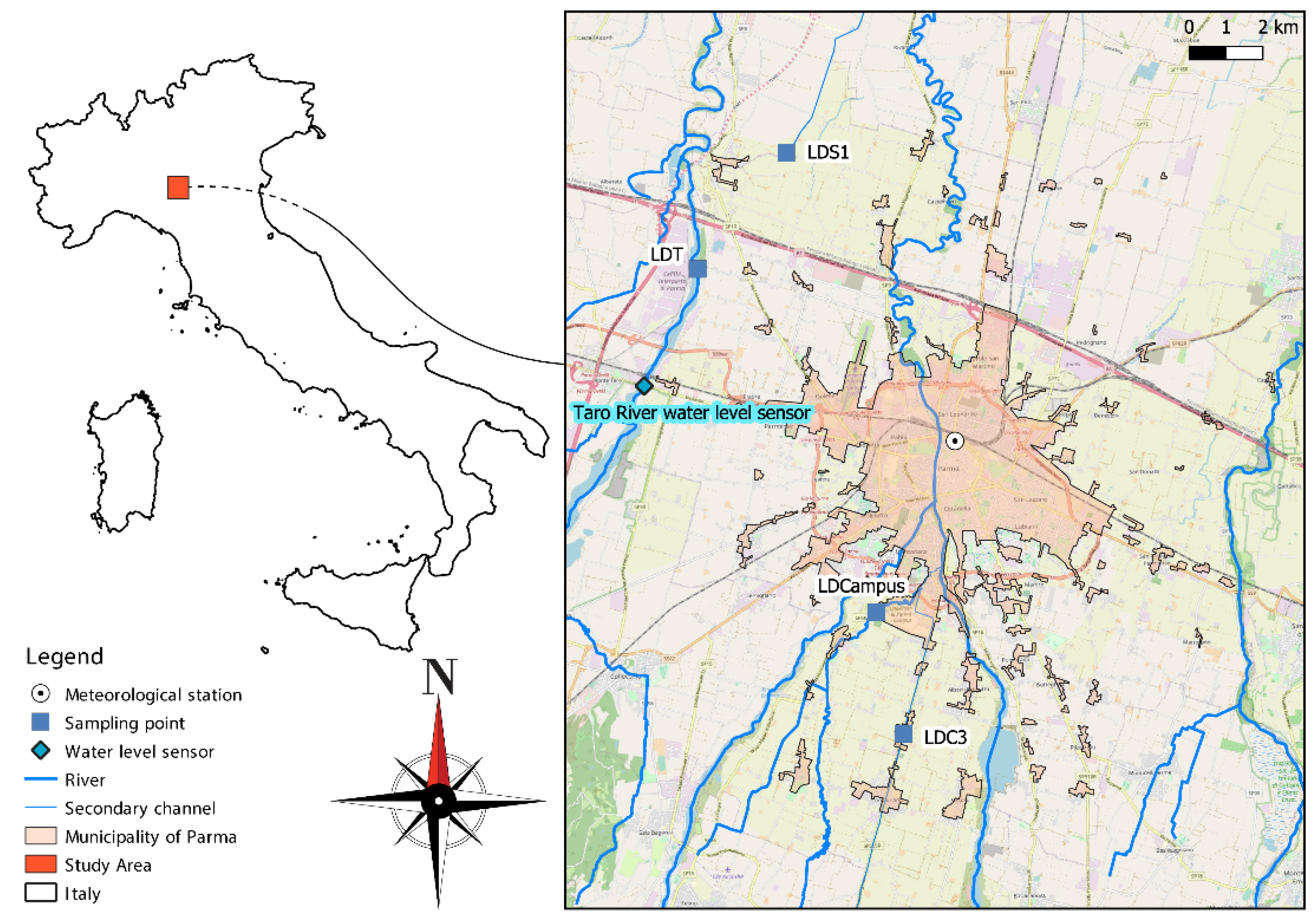
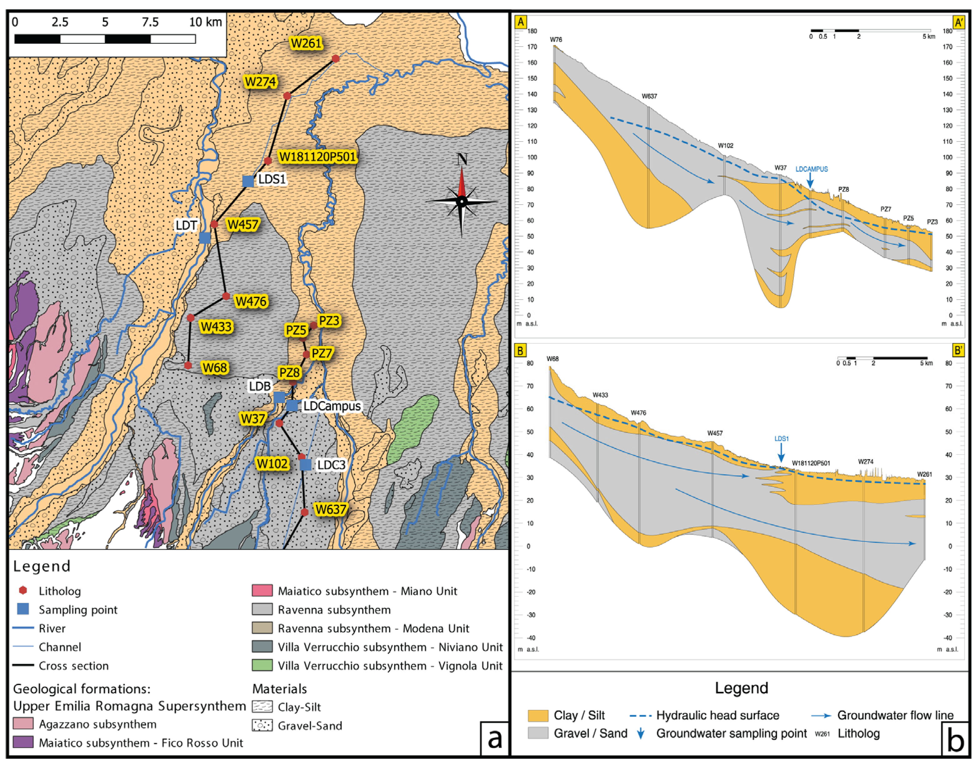
2.1. Study Area

This study was performed in an alluvial aquifer surrounding the city of Parma (Po Plain, Northern Italy, Figure 1). This area was selected due to its peculiar hydrogeological and anthropic characteristics. Intensive agriculture (mostly hay, tomatoes, and maize) results in numerous recognized sources of microplastics contamination [23]. The city of Parma is located in the center of the study area. It represents another possible important microplastics source for surface waters [24,25] and groundwater due to leaks in the drainage system [26,27]. Finally, the area has many large industrial complexes, another possible source of microplastics contamination [28], and is close to the so-called packaging valley, composed of more than 300 firms working in packaging and packaging machinery manufacturing and providing the biggest amount of industrial plastic wastes in the region [29]. All these factors can be expected to contribute to microplastic production and pollution [28]. Three rivers cross the area, namely the Taro, Baganza, and Parma River. The last two merge within the Parma city area and all of them flow into the River Po, the largest Italian river.

From the (hydro)geological perspective, the area has already been characterized by Zanini et al. [30], while several Master Theses of the University of Parma investigated some phenomena at small scale, e.g., [31,32]. The area is characterized by the Emilia-Romagna Supersynthem (Lower Pleistocene, about 800 ky BP to present), made up of fan and alluvial plain deposits, together with intravalley and terrace deposits. The grain size of the sediments is highly variable, resulting in the juxtaposition of more-permeable layers (gravel and sand) with low-permeability layers (clay and silt) [30]. The same authors tested the hydraulic conductivity of these layers in the wells of the Parma University Campus (which includes the piezometer LDCAMPUS used within this study). A pumping test performed in the more-permeable layer resulted in transmissivity and storativity of 3 × 10⁻⁴ m²/s and 1.9 × 10⁻⁴, respectively. In the low-permeability layer, the hydraulic conductivity was lower (in the order of 10⁻⁷/10⁻⁹ m/s) and estimated using a Lefranc test. Granulometric data of a litholog near LDCAMPUS (3.8 km N-E, Figure S1, Tables S1 and S2) is reported in the supplementary material and provides another piece of evidence of the low permeability of the confining unit.

2.2. Data Acquisition and Microplastics Sampling

The geological contextualization performed by Zanini et al. [30] was spatially expanded using stratigraphic data from the Geognostic tests database of the Emilia-Romagna Region [33] and Petrucci et al. [34], together with outcropping data from the Geological map of the Emilia-Romagna Region, 1:25,000 scale [35]. Near the sampling points, a detailed reconstruction of outcropping materials and shallow aquifer architecture was performed using geophysical investigations (i.e., resistivity imaging) from Francese et al. [36]. These helped to verify the confined or unconfined conditions of the aquifer. Finally, these data were used to identify two subareas to evaluate the effect of river–groundwater interaction and aquifer recharge on microplastics contamination in groundwater.

Water samples were collected from four stations during a small recession phase (25 March 2021), interrupted by a recharge event (13 April 2021) (Figure S2). A complete representation of hydraulic head variations during the hydrologic year in LDCAMPUS is reported in Figure S3. During both sampling periods, two surface-water samples were collected, namely LDT (sampling point in the Taro River) and LDC3 (sampling point in the La Riana Channel). The other two samples were collected from groundwater, namely LDCAMPUS (piezometer) and LDS1 (natural spring). The sampling time was established using precipitation data (Parma meteorological station, Figure 1) and data of the Taro River flow (Taro River water-level sensor, Figure 1), obtained from the Regional Environmental Protection Agency of Emilia-Romagna (ARPAE) website [37]. In addition, piezometric heads in LDCAMPUS were measured using a pressure transducer with a data logger (STS DL.OCS/N/RS485). The LDCAMPUS piezometer is composed of a 3 in. polyvinyl chloride (PVC) tube reaching 30 m bgl (below ground level) and screened between 23.80 and 26.80 m bgl. The piezometer stratigraphy data begins with deposits made by silt and clay from 0 to 4.90 m bgl. Below this horizon lies the confined “shallow aquifer” (from 4.90 to 26.70 m bgl), which is mainly made of gravels with rare and thin clay lenses. From 26.70 m bgl, other deposits made by silt and clay are found and the piezometer ends at 30.00 m bgl.

All water samples were taken and processed with glass or metallic tools and instruments to avoid contamination, except for the hydrogen peroxide (H₂O₂) container which was made of plastic (High-density polyethylene, HD-PE). In surface (and spring) water, 5 L samples were taken using a glass beaker at different depths (surface, medium, bottom) near the riverbank and stored in glass bottles with cork tops. All material was rinsed with Milli-Q water before sampling. A metallic Bailer (250 mL) with a metallic wire was used in the piezometer. Groundwater was not purged before sampling to avoid contamination from the plastic tube of the water pump. The bailer sampler was used to sample groundwater at groundwater/air interface and at medium height, but not at the piezometer bottom to avoid contamination from the piezometer tube made of PVC, which fragments (with density up to 1.37 g/cm³) fall to the bottom of the water column. A total of 5 L of groundwater was stored and processed in the same manner as for surface waters. The sample amount was decided based on different needs: The first is to maximize the number of possible microplastics found sampling a higher volume, which is usually between 0.5 and 2 L [20,22,38]. The second is to sample a sufficiently, yet easily transported and stored, large volume. Thus, the final sample volume was set to 5 L for both surface and groundwater, making them also more comparable. Although final values are reported as microplastics per liter (microplastics/L), the treatment of different volumes entails the use of different amounts of reagents, making the comparison between processed surface water, groundwater, and analytical blank samples (5 L of Milli-Q) meaningless.

Together with microplastics, other samples were taken for isotopic analysis (³H, δD‰, and δ¹⁸O‰), to evaluate the effect of a recharge event. The analyses for the determination of the tritium activity were carried out according to the procedures provided by the International Atomic Energy Agency [39] at the Isotope Geochemistry Laboratory at the University of Trieste (Italy). The analytical prediction uncertainty was ±0.5 TU. Stable isotope analyses (δD‰ and δ¹⁸O‰) were performed at the Isotope Geochemistry Laboratory at the University of Parma (Italy), using a Delta Plus mass spectrometer (Thermo Fisher Scientific, Waltham, MA, USA) coupled to an automatic HDO device preparation system. In the field, temperature, dissolved oxygen (O₂ mg/L and O₂%), electrical conductivity (EC), Oxidation Reduction Potential (ORP), and pH were measured using a multiparameter probe (HI9829 HANNA Instruments, Woonsocket, RI, USA), calibrated the day before sampling. These measurements were not performed in LDT (Taro River) due to logistic problems with the probe.

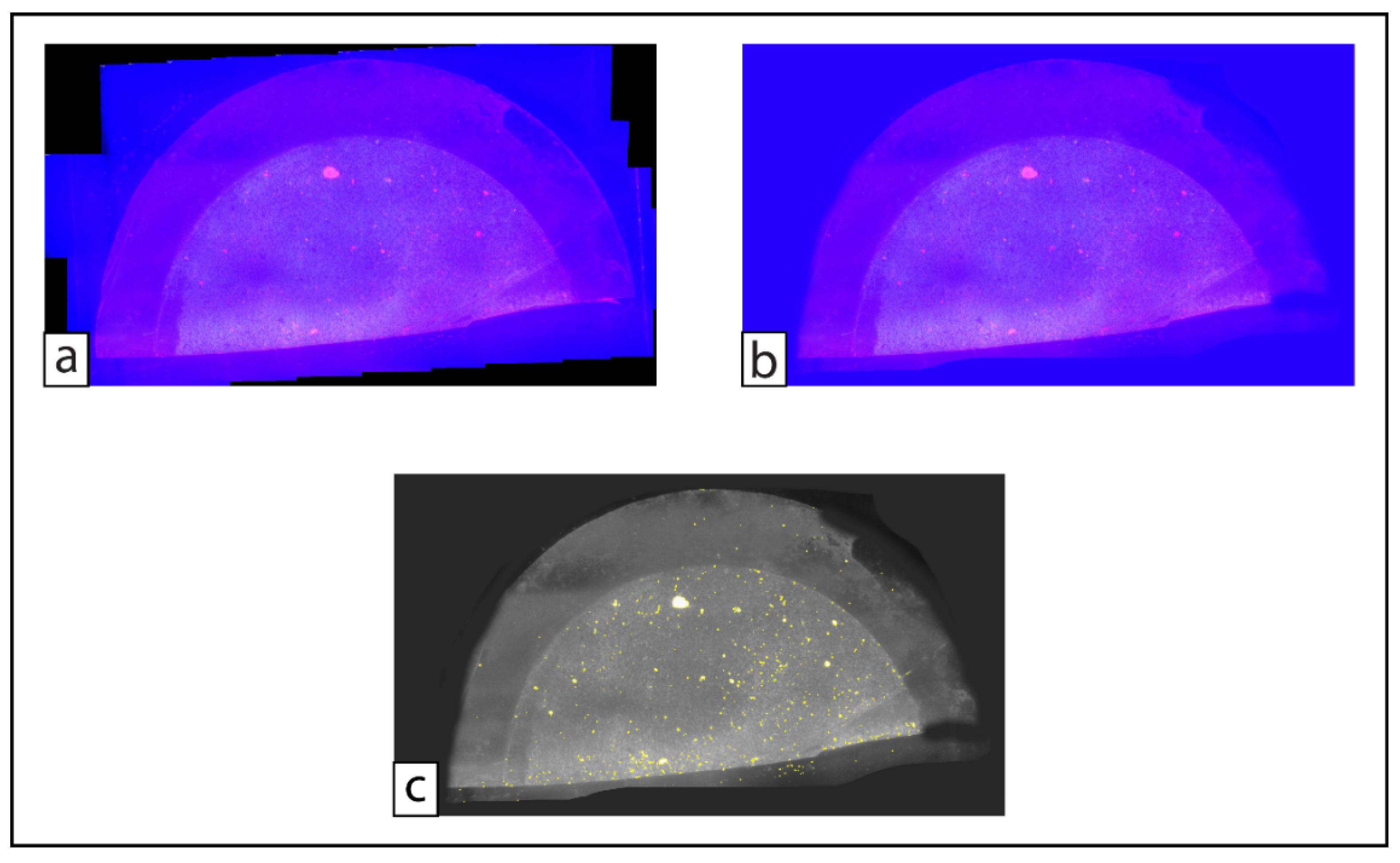
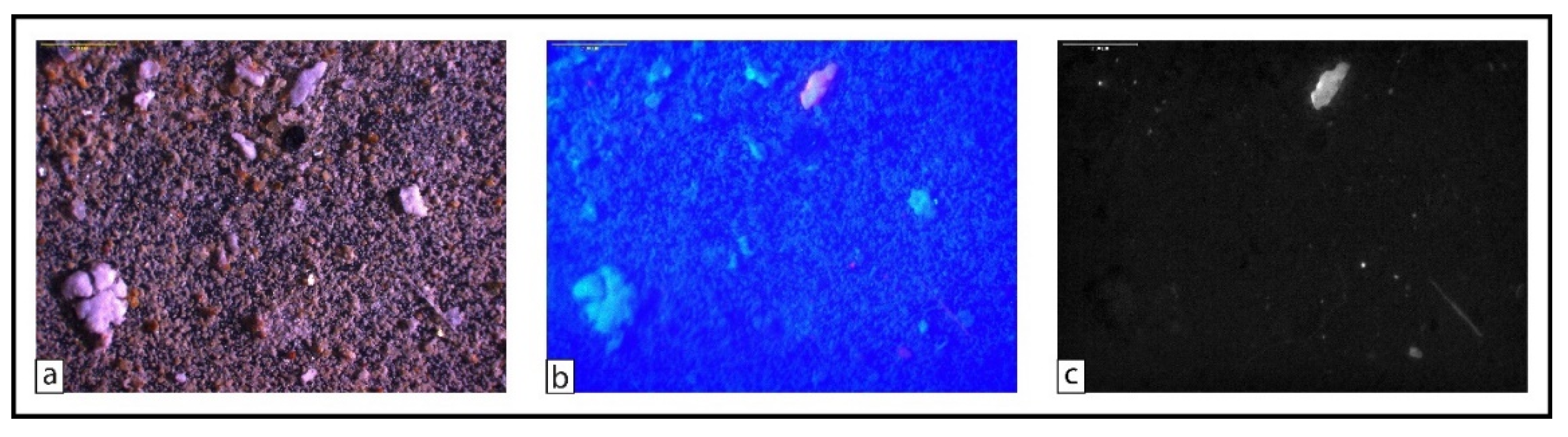
2.3. Microplastics Extraction and Processing

The 5 L samples were processed after 24 h, to allow the sedimentation of suspended materials. After that, the supernatant and suspended solids were filtered on polycarbonate track-etched (PCTE) filter membranes (47 mm diameter and 10 μm pore diameter, Steriltech Corporation). Although PC is a plastic material, the hydrophilic surface of the filters prevents its staining, also avoiding false positives from filter particles. Between 2 and 7 membranes were used per sample, according to the suspended solid load. Bottles and vacuuming gear were rinsed thoroughly with Milli-Q water (Millipore, Bedford, MA, USA) before and after every sample to avoid contamination. The filter membranes were left covered in an oven until dry [40]. The digestion of organic material was performed after drying by placing the membranes in 20 mL of 30% H₂O₂, followed by further oven drying [40]. Once dried, the membranes were carefully washed with Milli-Q water using in the same beaker and checked using backlighting for possible residuals. Filters were again placed in the oven until dry. After desiccation, the solid sample was rinsed with a high-density floatation solution (5.57 M) of K₂CO₃ (≥99.0%, VWR Chemicals) for microplastic isolation [41]. The samples were poured into density-separation glass funnels for the separation of sediments (denser) from microplastics (less dense). The lower-laying sediments were eliminated from the funnel and the K₂CO₃ solution was retrieved for future use [41]. The upper liquor was filtered over a single PCTE filter and Milli-Q water was used to carefully wash the remaining microplastics from the funnels. After that, the filter was dried at ambient temperature in a covered glass Petri dish.

A 1 mg/L solution of Nile Red (Fisher Scientific) and methanol (≥99.8%, VWR Chemicals) was prepared just before the microscopic analysis, according to Erni-Cassola et al. [40]. After applying a few drops (3 to 4) to cover the filter, they were cut in half using a scalpel blade (previously rinsed with Milli-Q) to fit over standard microscope slides and stage, covered with coverslips, and fixed with tape. The samples were stored at 60 °C for 10 min in the dark. A stereomicroscope (Leica S8AP0) was equipped with a camera (Leica DFC295 with Leica Application Suite, version 4.2.0), an external fluorescence light source (excitation 470 nm, royal blue), and an orange photography filter [40,42]. Microscopy images were taken using exposure times between 0.7 s and 1 s. Several images were taken for every filter, usually overlapping by around 30% to enable reconstruction of the panoramic view of the filter, using the demo version of Autostitch [43]. A minimum background signal (e.g., fine sediments on the filter) must be provided, for the program to reconstruct the image correctly and to avoid distorted outputs. After the reconstruction, ImageJ (version 1.53, [44]), was used to perform automated particle recognition and quantification based on the fluorescent particles using parameters similar to Erni-Cassola et al. [40] and Prata et al. [45]. After the automated quantification of microplastics, an output is produced by ImageJ, in which the microplastics selected in the red channel are highlighted in yellow. This final image is inspected for false-positives or errors (see Section 4.1). The ImageJ script was tested using artificially made filter images (Figure S4). A more detailed description of the protocol and the specifications used in both Autostitch and ImageJ is reported in the Supplementary Material, together with QA/QC measures derived from Erni-Cassola et al. [40] and Koelmans et al. [46]. Simultaneously, three replicates of 5 L Milli-Q water were analyzed as control samples (blanks), using the same procedure described above. The resulting analytical contamination was used to set the ImageJ parameters for plastics identification. Since the control samples were contaminated by microplastics with lower area and higher circularity than those from the environmental samples, these were excluded by the ImageJ identification imposing those values as limits for the particle identification (see Section 3.2 and Section 4.1). Thus, in the environmental sample, only microplastics with a lower circularity and higher area of the median value of those in the control samples were counted and characterized. Besides the count of the fluorescent microplastics, the used ImageJ protocol allows for the quantification of important features such as the microplastics area (μm²), Feret diameter (μm), and circularity, which is expressed in a number between 0 (low) and 1 (high). Statistical analysis of these results was performed using the statistics software R [47]. The statistical approach was chosen to verify possible differences in the above-mentioned geometrical parameters between the samples and sampling time (i.e., after the recharge event). Differences among controls (Ctrl), groundwater (GW), and surface-water samples (SW) were tested using the Kruskal test [48] using the package “Rstatix” [47]. If significant, Dunn’s post hoc test was performed [49] through the R package “FSA” [50], using the Benjamini–Hochberg method for adjusted p values. Differences among groundwater (GW) and surface-water samples (SW), together with differences among the sampling times, were tested using the Mann–Whitney U test [51]. On the contrary, since data were normally distributed, the abundances between the two sampling times were compared using the paired t-test [51]. Both statistical tests were chosen based on the sampling design, together with verified and nonverified assumptions.

3. Results

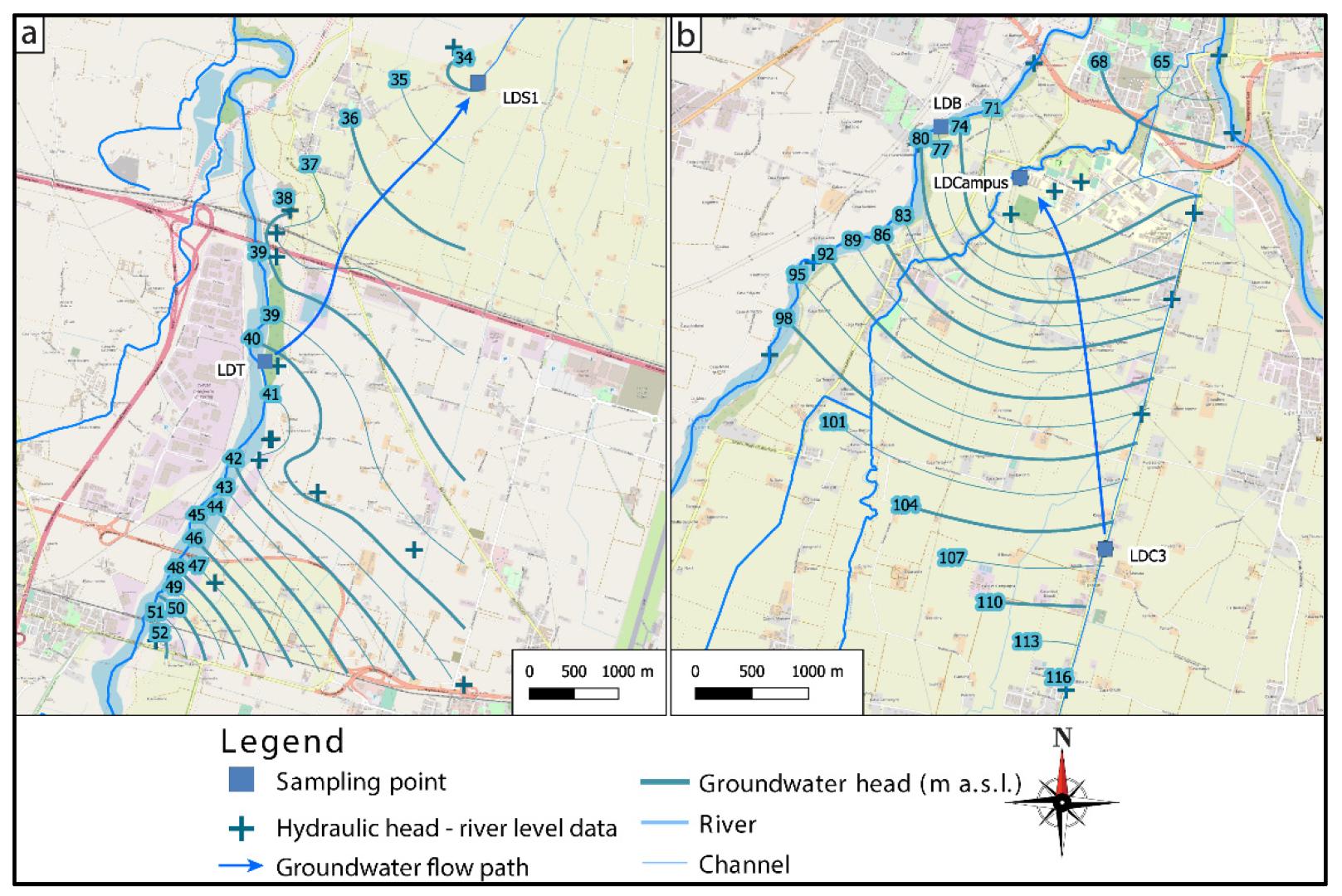
3.1. Hydrogeological Features of the Study Area and the Effects of Aquifer Recharge

A detailed hydrogeological characterization of the investigated area is presented in Figure 2. The outcropping sediments are related to the Ravenna Subsynthem (AES8) and the Modena Unit (AES8a) [52]. The Ravenna Subsynthem (originated between the upper Pleistocene and Holocene) primarily comprises sandy gravel, sand, and stratified silt, with a discontinuous cover of clayey silt. The Modena Unit (originated during the Holocene) primarily comprises sands with gravel lenses, covered by a discontinuous layer of clayey silt [52]. The outcropping materials were grouped based on their relative permeability. More permeable outcropping (gravel and sand) is found in the southwest part of Figure 2 (near the foothill) and nearby the main watercourses, while the less-permeable outcroppings (clay and silt) are reported in the northeast part of Figure 2. Thus, the aquifer is identified as unconfined at the southwest and near the Taro River, which dissected the clay and silt cover. On the contrary, it is identified as confined in the remaining area (northeast), where the confining (clay and silt) layer can reach 15 m of thickness (litholog W181120P501).

The points in the two subareas where sampling was performed are also reported in Figure 2. Each one is composed of one (or two) sampling points for surface waters and another one for groundwater. The first subarea is in the central part of Figure 2. It is composed of a losing channel (namely LDC3), a losing stream (LDB), and a piezometer downgradient (LDCAMPUS, Figure 3a). Within these points, the aquifer changes from unconfined to confined. The hydraulic head of the pressure transducer in the LDCAMPUS piezometer showed a recession period of groundwater interrupted by a recharge event (Figure S1). The aquifer recharge supplied by rain results in a small rise of the hydraulic head. This phenomenon, although of small entities, is appreciable also in the previous (small) recharge events (Figures S1 and S3). The fast response of the system provides other pieces of evidence to the high permeability of the surrounding area. Without the recharge event, the hydraulic head would keep lowering with a regression coefficient of 0.015 d⁻¹. The recharge resulted also in a variation of EC (

Table 1. Isotopic and field data. The dot represents not-analyzed samples.

Date	Sample	t (°C)	O2 (mg/L)	O2 (%)	EC (μS/cm)	ORP (mV)	pH	3H (TU)	δD‰ (vs V-SMOW)	δ18O‰ (vs V-SMOW)
25 March 2021	LDS1	14.0	2.99	29	586.1	89.8	7.6	7.06	−45.10	−7.44
25 March 2021	LDCAMPUS	16.0	8.51	87	893.0	201.5	7.3	-	-	-
25 March 2021	LDC3	6.4	8.96	73	608.7	143.1	8	-	-	-
13 April 2021	LDS1	14.0	2.08	20	577.5	154.9	7.3	9.30	−43.80	−7.42
13 April 2021	LDC3	7.7	9.22	77	467.7	139.5	8	-	-	-
13 April 2021	LDCAMPUS	14.0	7.67	81	308.4	190.2	6.9	-	-	-
13 April 2021	Precipitation	-	-	-	-	-	-	10.00	-	−13.2

). In both LDC3 and LDCAMPUS, the EC values were lower after the recharge given by precipitation. This evidence is consistent with the conceptualized river–groundwater interaction, with LDC3 feeding LDCAMPUS.

The water level of the Taro River rapidly increased after rainy days. Therefore, the discharge of LDS1 increased, due to the high groundwater recharge provided by the Taro River (Figure 3b). The spring discharge was not measured during the first sampling due to the low flow and incompatibility with the current meter (Small Current Meter C2, OTT, Kempten, Germany). After the recharge event consequent to the flow rise in the Taro River, the spring discharge raised from nonmeasurable to 4.8 L/s. The recharge effect on LDS1 is evident also in tritium content (Table 1). After the recharge event, the tritium content of the spring increased by 31.7% (+2.24 TU) and was closer to the tritium content of precipitation. Thus, the tritium content of LDS1 over time is consistent with the proposed river–groundwater interaction, with LDT feeding LDS1. These data also testify that the groundwater flow nets reconstructed with data from [30,31,32] are still valid, at least in the investigated subareas. Unlike for surroundings of LDCAMPUS, no data about hydraulic conductivity and storativity are available for this subarea. Nevertheless, given the fast response of the spring to the recharge, and the comparable grain size of the aquifer, we assumed that hydraulic conductivity is like that of the area near LDCAMPUS, in the order of 10⁻⁴ m/s.

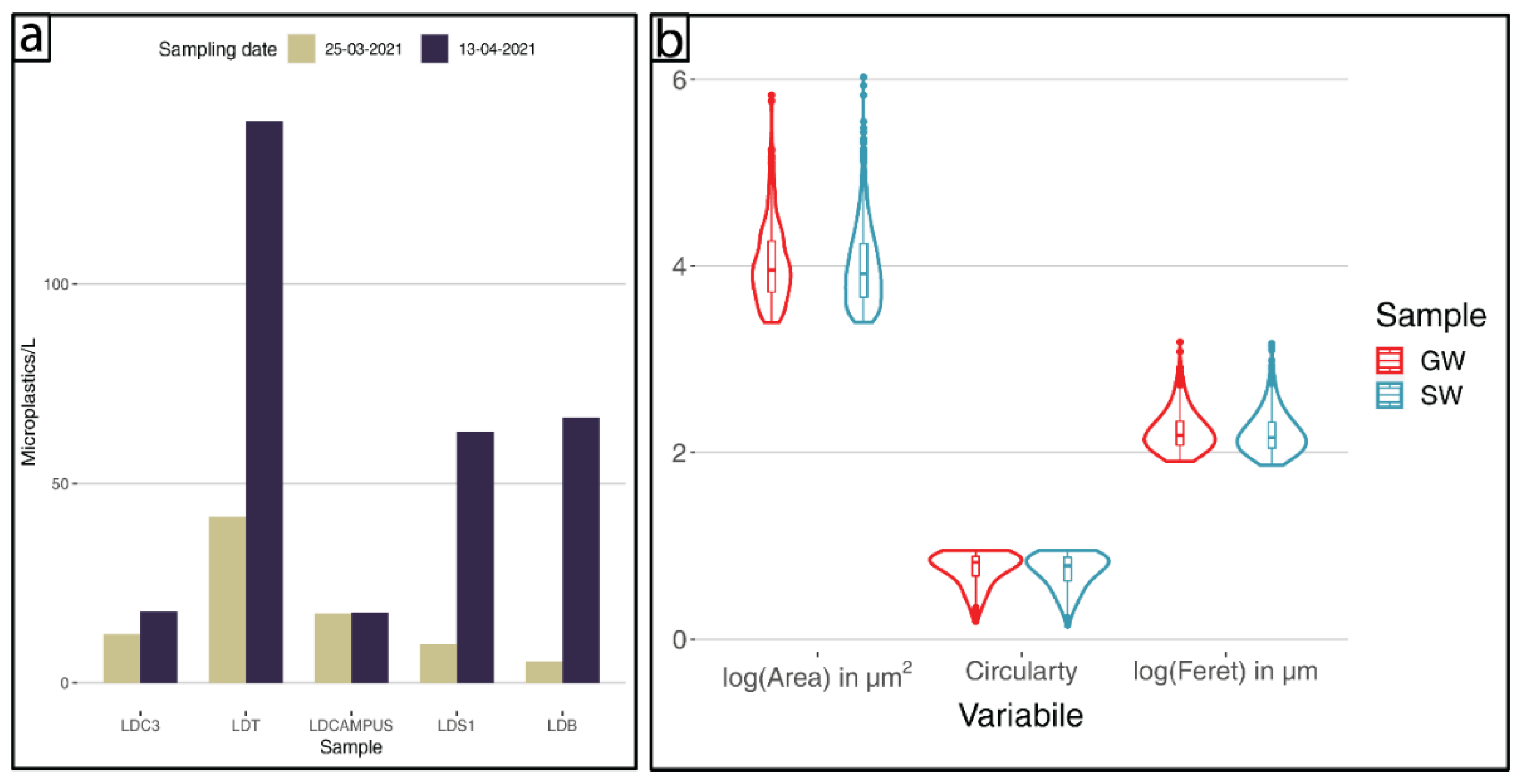
3.2. Microplastics Quantification and Geometric Characterization

To reconstruct the whole panoramic view of the filters, typically 45 ± 11.4 (average ± standard deviation) photos were taken for every microscope slide, i.e., half-filter. The maximum number of photos taken was 76, while the lowest was 29. In total, 989 photos were taken. The microplastics’ presence in both surface and groundwater was highly heterogeneous. Surface-water samples showed a large range of values, with a mean concentration of 47.4 ± 51 microplastics/L, while the groundwater samples’ mean was 26.88 ± 24.37 (Figure 4). The concentration of analytical and field samples is reported in Table S3. All the samples showed an increase in microplastics concentrations after the recharge event.

Regarding the geometrical characterization, control and environmental samples showed interesting and peculiar characteristics. A statistical difference was reported between microplastics in both environmental samples and analytical blanks, not only in the area (Chi square = 140.31, df = 2, p value = 2.2 × 10⁻¹⁶), but also in circularity (Chi square = 74.415, df = 2, p value = 2.2 × 10⁻¹⁶) and in the Feret diameter (Chi square = 152.86, df = 2, p value = 2.2 × 10⁻¹⁶). These differences were further tested using the Dunn’s test for pairwise comparison, showing that microplastics in control samples had a smaller area and Feret diameter than surface and groundwater samples, while the circularity was higher in control samples (Tables S3 and S4). This information justified the setting of an identification limit for environmental samples’ microplastics equal to the median value of the analytical blanks’ microplastics to avoid their overestimation. However, this is expected to result in an underestimation of sample microplastics with dimensions and characteristics in the range excluded during image analysis. While an underestimate is not ideal, it is acceptable, to account for the observed levels of contamination. After this, the environmental samples were analyzed again with the new parameters to exclude the laboratory contamination, and the differences between surface waters and groundwater were tested using Mann–Whitney U test. The results revealed a higher circularity and Feret diameter in groundwater than in surface waters, whereas no difference was reported for the area (Table S3). The geometrical features of microplastics were also tested between the two sampling times (before and after the recharge event). As a result, the Mann–Whitney U test highlighted a significant difference between the sampling times in circularity for surface water samples (W= 149608, p value = 1.17 × 10⁻²), whereas no other difference was statistically significant (Tables S3 and S4).

4. Discussion

4.1. Assets and Disadvantages of the Extraction Protocol

The proposed sampling strategy aimed to avoid contamination during sampling by using only metallic or glass tools. Sampling with the metallic Bailer can be more time-consuming than the direct sampling with a beaker. This is in any case dependent on the depth of piezometric level and the Bailer volume.

The methodology used for microplastics extraction, derived from the integration of previously reported methods, allowed a good characterization of the microplastics contamination through an inexpensive and easily performable procedure. Although microplastics analysis through fluorescence has already been reported as a successful method [53], some improvements were adopted. Starting from the protocol proposed in Erni-Cassola et al. [40], a higher number of filters was used for every sample during the first filtration step. This is due to the high load of suspended solids found in surface waters during the recharge event, which happened to obstruct the filter and possibly cover microplastics with silt and clay, which were difficult to remove from the final processed sample (Figure 5). The high amounts of suspended solids also made the use of a floatation solution for microplastic unavoidable. To also allow the isolation of denser microplastics such as PVC, a 5.57 M solution of potassium carbonate (K₂CO₃) was prepared, with a density of 1.54 g/cm³. This particular floatation solution was preferred to others such as ZnCl and NaI, as K₂CO₃ is cheaper, recyclable, and more environmentally friendly [41], while having a higher density than the NaCl solutions (up to 1.2 g/cm³).

In addition, high-density solutions of K₂CO₃ can easily precipitate [41], forming crystals in the final processed sample. Despite that, these crystals had no consequences during fluorescence analyses (Figure 6), since they have no red color and were well-eliminated from the image during the color-splitting step in ImageJ (see detailed analysis protocol in the Supplementary Material). These macroscopic precipitates were associated with K₂CO₃ since they were not present in the previous stages of the analysis.

The filters were clipped in half as in Erni-Cassola et al. [40], but early cutting attempts of dry filters resulted in the loss of material. As an adjustment, filters were cut immediately after the Nile red solution application, which wetted the material over the filter and avoided its loss during the cutting phase. If used in a larger volume than necessary, it was observed that the Nile red solutions could dye the filter membrane’s borders. In this case, the filter image was modified in a raster graphics editor using a blue brush to correct these defects (Figure 7), which would otherwise be considered as microplastics by ImageJ. The blue color was preferred since it cannot result in false positives in ImageJ due to channel separation (see detailed analysis protocol in the Supplementary Material).

The use of microscope slides and coverslips was preferred to simply uncovered Petri dishes, for two reasons: firstly, they avoid laboratory contamination without lowering the image quality. Secondly, they allowed the inspection of the whole (half-)filter, conversely to Petri dishes whose edges would interfere with the microscope objective. The use of Petri dishes larger than the filter (47 mm diameter) was discouraged, as they could not steadily hold the filter during sample handling. The necessity to analyze the whole filter, instead of some random parts of it, is derived from the microplastics distribution in the filter, which is not homogeneous. In fact, during the filtration process, it was observed that microplastics did stick to the internal walls of the filtration unit. After rinsing, they were more concentrated on the external area of the filter. In addition, more microplastics were also found in the central part of the filter, where the first spilled sample was filtered. For these reasons, the use of randomly taken images was avoided and an accurate, albeit more time-consuming, reconstruction of the whole filter image was performed using the demo version of Autostitch, as reported in Maes et al. [43], using images taken through a microscope and resulting in a higher resolution with a theoretical smaller minimum dimension of particles for detection.

The microscope adaptations proposed by Labbe et al. [42] were successfully replicated and utilized for the analyses presented in this study. Although a high number of microplastics was detected, the comparison between normal light and the final output of the identification procedure (Figure 6) showed a lower sensitivity for microplastics of elongated and thin shape such as fibers, which were not detected for their whole length but only for portions of it. Lastly, the microscope adaptation was realized with a very low budget (<100 EUR). The main issue with microplastics analysis is often laboratory contamination and usually other studies focus on the extent of contamination alone [22,40]. On the contrary, in this method, the contamination was excluded by setting the ImageJ macro to identify and characterize microplastics different from those found in the analytical blanks, which were characterized by a (statistically significant) lower area and Feret diameter but a higher circularity than those in environmental samples. As a result, the laboratory contamination is no longer a major issue, although this implies the noncharacterization of smaller microplastics, and of those with size and geometries similar to those of analytical blanks, resulting in a likely underestimate. The possible sources of contamination were identified in unfiltered laboratory solutions and airflow (although AC was turned off or down during analyses). This was ascertained by testing the microplastics abundance in analytical blanks (5 L Milli-Q) analyzed using filtered (3x) and unfiltered (3x) reagents and Milli-Q. As a result, the analytical blanks analyzed using unfiltered reagents and Milli-Q had a mean contamination of 37.13 microplastics/L (respectively 35, 56.4, and 20 microplastics/L), whereas those analyzed using filtered reagents and Milli-Q showed significantly lower contamination (13.4, 6.4, and 35.6 microplastics/L, respectively), with a mean value of 18.4 microplastics/L. Moreover, the geometrical characteristics of microplastics were similar between the samples treated with filtered and unfiltered reagents and Milli-Q. This consideration supports the origin of microplastics’ contamination in unfiltered laboratory solutions, which could contain smaller microplastics than those in environmental solutions [45,54], with a possible more rounded shape due to the abrasive and smoothing effect of the used salts (i.e., K₂CO₃) in plastics packaging. The material (high purity grade) bought for the laboratory solutions was sold in plastic packages, except for Nile red. Hence, a prefiltration of all the used solutions should be performed before use [22,43,45]. Since it was not present in Erni-Cassola et al. [40], the refiltration was not performed before the analysis of the presented samples.

4.2. Aquifer Recharge and River–Groundwater Interaction as Drivers of the Microplastic Contamination

Microplastics were present in all the analyzed samples, providing further evidence of microplastics contamination in groundwater, of which studies are still rare. Groundwater samples showed a large range of particle concentrations (26.88 ± 24.37 microplastics/L) but had a lower mean particle concentration than surface-water samples (47.4 ± 51 microplastics/L), which also showed a large range of values, although the aquifer in the investigated subareas is fed by losing streams and channels. Hence, a filtering effect of the aquifer can be ascertained and its effects on microplastics contamination can be better clarified by looking at the geometries of microplastics found in groundwater. These had a higher circularity and Feret diameter than those in surface water. According to Pirard [55], the circularity parameter “lack[s] clear physical significance”, since it can be equal for very different shapes. Nevertheless, it is an optimal descriptor of the progressive change from any initial morphology, since it is the ratio of the microplastics’ projected area to that of a sphere projecting the same perimeter length. As such, this ratio is an adequate measure of the extent of transport processes, in which particles are expected to degrade toward sphericity [56,57]. Moreover, a more rounded shape fosters the transport of particles in porous media such as alluvial aquifers, as reported by Keller et al. [58] and by further authors for bacteria [59] and other colloidal materials [60,61]. In other words, microplastics found in groundwater are a subsample of those in surface waters, where only those that underwent prolonged transport processes (higher circularity) can be transported also into the aquifer and groundwater. The remaining part of microplastics in surface waters, which contribute to the higher concentration in surface waters, is constituted likely by mostly secondary microplastics, which did not yet undergo transport processes. The higher Feret diameter for microplastics in groundwater compared to those in surface waters is an unexpected result. We speculate that it is related to the presence in groundwater of microplastics with a more simplified shape than those in surface waters, e.g., untangled fibers or nylon fragments, which can be easily crinkled during the transport processes in surface waters. Nevertheless, these are just hypotheses, establishing new questions and encouraging further investigations about the effect of microplastics’ shapes during transport in porous media.

Regarding the effects of the recharge event, although a general increase in microplastics concentrations was found after precipitations, this difference was not statistically significant (Table S3). In the Taro River (LDT) and spring (LDS1) subarea, the increase in microplastics in groundwater is undeniable (Figure 4). On the other hand, the subarea with LDC3, LDCAMPUS, and LDB showed a lower increase in microplastics contamination after the recharge event. Hence, the effects of the recharge event can be detected only under certain circumstances. In both subareas, a higher microplastics contamination was expected due to the higher hydraulic head given by aquifer recharge. This process was investigated at laboratory scale in porous media by Bizmark et al. [62], who found that a higher pressure in the medium is responsible for an enhanced transport of colloidal particles such as microplastics. In addition, the higher discharge of the river and channel after precipitation leads to a highly unsteady flow regime, which promotes the resuspension and transport of deposited bottom sediments (and microplastics), the release of contaminants from the interstitial water of the sediments, and causes land erosion [63]. In the investigated area, only the Taro River (LDT) experienced a higher microplastics contamination after precipitation, whereas the channel (LDC3) experienced a smaller increase in microplastics contamination. The groundwater fed by these surface waters responded accordingly, and only in LDS1 was the microplastics concentration higher after the aquifer recharge. Due to the heterogeneity of surface-water contamination and relative recharge of groundwater, the difference between the sampling periods was not statistically significant. Nevertheless, these data prove that the processes described in Bizmark et al. [62] can be upscaled to a km scale and that the different entities of groundwater contamination should be compared only between the same groundwater flow path and systems when possible. The precipitation and consequent aquifer recharge did not promote any change in the geometrical parameters of microplastics, except for circularity in surface waters, characterized by a lower value after the recharge event. This fact is consistent with the above-mentioned dynamics and testifies that a phase of high river discharge fosters the formation of new or the resuspension of sedimented secondary microplastics, which are typified by a lower circularity value since they did not yet undergo prolonged transport processes. This does result in a rise in microplastics concentration, but this is not statistically significant (Table S3; Figure 4). It is in any case sufficient to lower the circularity median value of microplastics in surface waters.

5. Conclusions

The investigation was performed using a protocol based on a self-made fluorescence microscopy setup and an open-source image-processing program, resulting in a high result-to-cost ratio. Such a technique allows even those who lack access to a specialized analytical chemistry laboratory and high levels of contamination control measures to conduct research in this field. This will be particularly useful in developing countries, where the research in this field is less advanced than that in developed countries and complicated by potentially limited access to expensive equipment, e.g., micro-FTIR or micro-Raman [64].

In addition, the presented results shed new light on the interaction of microplastics’ abundance and geometrical attributes with the hydrogeological characteristics of the aquifer. Although not yet characterized from a chemical perspective, the microplastics observed in the samples provide valuable information regarding their presence and transport in a porous material, i.e., alluvial aquifer. Furthermore, these findings raise new and urgent questions about microplastics in groundwater. For example, which mechanisms influence the transport of microplastics in alluvial aquifers? How do the geometrical features of microplastics, coupled with their electrochemical characteristics, affect their transport in the aquifer? Extensive research is still required in this field, which is poorly explored and demands further attention by the scientific community.

References

1. Bergmann, M.; Gutow, L.; Klages, M. Marine Anthropogenic Litter; Springer Nature: Berlin/Heidelberg, Germany, 2015. [Google Scholar]
2. Arthur, C.; Baker, J.; Bamford, H. International research workshop on the occurrence, effects, and fate of microplastic marine debris. In Proceedings of the International Research Workshop on the Occurrence, Effects and Fate of Microplastic Marine Debris, Tacoma, WA, USA, 9–11 September 2008. [Google Scholar]
3. Hartmann, N.B.; Hüffer, T.; Thompson, R.C.; Hassellöv, M.; Verschoor, A.; Daugaard, A.E.; Rist, S.; Karlsson, T.; Brennholt, N.; Cole, M.; et al. Are We Speaking the Same Language? Recommendations for a Definition and Categorization Framework for Plastic Debris. Environ. Sci. Technol. 2019, 53, 1039–1047. [Google Scholar] [CrossRef] [PubMed] [Green Version]
4. Cole, M.; Lindeque, P.; Halsband, C.; Galloway, T.S. Microplastics as contaminants in the marine environment: A review. Mar. Pollut. Bull. 2011, 62, 2588–2597. [Google Scholar] [CrossRef] [PubMed]
5. Gregory, M.R. Plastic scrubbers’ in hand cleansers: A further (and minor) source for marine pollution identified. Mar. Pollut. Bull. 1996, 32, 867–871. [Google Scholar] [CrossRef]
6. Zitko, V.; Hanlon, M. Another source of pollution by plastics: Skin cleaners with plastic scrubbers. Mar. Pollut. Bull. 1991, 22, 41–42. [Google Scholar] [CrossRef]
7. Browne, M.A.; Galloway, T.; Thompson, R. Microplastic--an emerging contaminant of potential concern? Integr. Environ. Assess. Manag. 2007, 3, 559–561. [Google Scholar] [CrossRef] [PubMed]
8. Thompson, R.C.; Olson, Y.; Mitchell, R.P.; Davis, A.; Rowland, S.J.; John, A.W.G.; McGonigle, D.; Russell, A.E. Lost at Sea: Where Is All the Plastic? Science 2004, 304, 838. [Google Scholar] [CrossRef]
9. Geyer, R.; Jambeck, J.R.; Law, K.L. Production, use, and fate of all plastics ever made. Sci. Adv. 2017, 3, e1700782. [Google Scholar] [CrossRef] [Green Version]
10. Iwata, T. Biodegradable and Bio-Based Polymers: Future Prospects of Eco-Friendly Plastics. Angew. Chem. Int. Ed. 2015, 54, 3210–3215. [Google Scholar] [CrossRef]
11. Wei, X.-F.; Bohlén, M.; Lindblad, C.; Hedenqvist, M.; Hakonen, A. Microplastics generated from a biodegradable plastic in freshwater and seawater. Water Res. 2021, 198, 117123. [Google Scholar] [CrossRef]
12. Barnes, D.K.A.; Galgani, F.; Thompson, R.C.; Barlaz, M. Accumulation and fragmentation of plastic debris in global environments. Philos. Trans. R. Soc. B Biol. Sci. 2009, 364, 1985–1998. [Google Scholar] [CrossRef] [Green Version]
13. Moore, C.J. Synthetic polymers in the marine environment: A rapidly increasing, long-term threat. Environ. Res. 2008, 108, 131–139. [Google Scholar] [CrossRef] [PubMed]
14. Carpenter, E.J.; Anderson, S.J.; Harvey, G.R.; Miklas, H.P.; Peck, B.B. Polystyrene spherules in coastal waters. Science 1972, 178, 749–750. [Google Scholar] [CrossRef] [PubMed]
15. Colton Jr, J.B.; Knapp, F.D.; Burns, B.R. Plastic particles in surface waters of the Northwestern Atlantic. Science 1974, 185, 491–497. [Google Scholar] [CrossRef] [PubMed]
16. Eerkes-Medrano, D.; Thompson, R.C.; Aldridge, D.C. Microplastics in freshwater systems: A review of the emerging threats, identification of knowledge gaps and prioritisation of research needs. Water Res. 2015, 75, 63–82. [Google Scholar] [CrossRef] [PubMed]
17. Li, J.; Liu, H.; Paul Chen, J. Microplastics in freshwater systems: A review on occurrence, environmental effects, and methods for microplastics detection. Water Res. 2018, 137, 362–374. [Google Scholar] [CrossRef]
18. Wagner, M.; Scherer, C.; Alvarez-Muñoz, D.; Brennholt, N.; Bourrain, X.; Buchinger, S.; Fries, E.; Grosbois, C.; Klasmeier, J.; Marti, T.; et al. Microplastics in freshwater ecosystems: What we know and what we need to know. Environ. Sci. Eur. 2014, 26, 12. [Google Scholar] [CrossRef] [Green Version]
19. Schmoll, O.; Howard, G.; Chilton, J.; Chorus, I.; World Health Organization; Water, Sanitation and Health Team. Protecting Groundwater for Health: Managing the Quality of Drinking-Water Sources; Schmoll, O., Howard, G., Chilton, J., Chorus, I., Eds.; IWA Publishing: London, UK, 2006. [Google Scholar]
20. Panno, S.V.; Kelly, W.R.; Scott, J.; Zheng, W.; McNeish, R.E.; Holm, N.; Hoellein, T.J.; Baranski, E.L. Microplastic Contamination in Karst Groundwater Systems. Groundwater 2019, 57, 189–196. [Google Scholar] [CrossRef]
21. Goeppert, N.; Goldscheider, N. Experimental field evidence for transport of microplastic tracers over large distances in an alluvial aquifer. J. Hazard. Mater. 2021, 408, 124844. [Google Scholar] [CrossRef]
22. Samandra, S.; Johnston, J.M.; Jaeger, J.E.; Symons, B.; Xie, S.; Currell, M.; Ellis, A.V.; Clarke, B.O. Microplastic contamination of an unconfined groundwater aquifer in Victoria, Australia. Sci. Total Environ. 2022, 802, 149727. [Google Scholar] [CrossRef]
23. Qi, R.; Jones, D.L.; Li, Z.; Liu, Q.; Yan, C. Behavior of microplastics and plastic film residues in the soil environment: A critical review. Sci. Total Environ. 2020, 703, 134722. [Google Scholar] [CrossRef]
24. Mani, T.; Hauk, A.; Walter, U.; Burkhardt-Holm, P. Microplastics profile along the Rhine River. Sci. Rep. 2015, 5, 17988. [Google Scholar] [CrossRef] [PubMed]
25. Peng, G.; Xu, P.; Zhu, B.; Bai, M.; Li, D. Microplastics in freshwater river sediments in Shanghai, China: A case study of risk assessment in mega-cities. Environ. Pollut. 2018, 234, 448–456. [Google Scholar] [CrossRef]
26. Ngo, P.L.; Pramanik, B.K.; Shah, K.; Roychand, R. Pathway, classification and removal efficiency of microplastics in wastewater treatment plants. Environ. Pollut. 2019, 255, 113326. [Google Scholar] [CrossRef] [PubMed]
27. Chen, H.; Jia, Q.; Zhao, X.; Li, L.; Nie, Y.; Liu, H.; Ye, J. The occurrence of microplastics in water bodies in urban agglomerations: Impacts of drainage system overflow in wet weather, catchment land-uses, and environmental management practices. Water Res. 2020, 183, 116073. [Google Scholar] [CrossRef] [PubMed]
28. Karbalaei, S.; Hanachi, P.; Walker, T.R.; Cole, M. Occurrence, sources, human health impacts and mitigation of microplastic pollution. Environ. Sci. Pollut. Res. 2018, 25, 36046–36063. [Google Scholar] [CrossRef]
29. Foschi, E.; D’Addato, F.; Bonoli, A. Plastic waste management: A comprehensive analysis of the current status to set up an after-use plastic strategy in Emilia-Romagna Region (Italy). Environ. Sci. Pollut. Res. 2021, 28, 24328–24341. [Google Scholar] [CrossRef]
30. Zanini, A.; Petrella, E.; Sanangelantoni, A.M.; Angelo, L.; Ventosi, B.; Viani, L.; Rizzo, P.; Remelli, S.; Bartoli, M.; Bolpagni, R.; et al. Groundwater characterization from an ecological and human perspective: An interdisciplinary approach in the Functional Urban Area of Parma, Italy. Rend. Lincei. Sci. Fis. E Nat. 2019, 30, 93–108. [Google Scholar] [CrossRef]
31. Viani, L. Idrodinamica Sotterranea Dell’acquifero Eterogeneo nel Parmense, Emilia-Romagna. Master’s Thesis, University of Parma, Parma, Italy, 2017. [Google Scholar]
32. Lancini, J. Studio IDROGEOLOGICO in Area di Discarica: Il CASO del sito “Area Vasta di Viarolo” (PR). Master’s Thesis, University of Parma, Parma, Italy, 2019. [Google Scholar]
33. Geognostic Tests Database of the Emilia-Romagna Region. 2020. Available online: https://ambiente.regione.emilia-romagna.it/it/geologia/cartografia/webgis-banchedati/banca-dati-geognostica (accessed on 23 February 2021).
34. Petrucci, F.; Bigi, B.; Morestori, L.; Panicieri, E.; Pecorari, M.; Valloni, R. Ricerca C.N.R. Sulle Falde Acquifere Profonde Della Pianura Padana: Provv. di Parma e Piacenza (Destra T. Nure) Dell’istituto di Ricerca Sulle Acque—I.R.S.A.; Istituto di Ricerca Sulle Acque—I.R.S.A.: Roma, Italy, 1975; Volume 1, p. 306. [Google Scholar]
35. Geological map of the Emilia-Romagna Region. 2004. Available online: https://ambiente.regione.emilia-romagna.it/it/geologia/cartografia/webgis-banchedati/webgis (accessed on 23 February 2021).
36. Francese, R.; Chelli, A.; Molinari, F.C.; Paini, M. Microzonazione Sismica: Relazione illustrativa. Studio di Microzonazione Sismica di II Livello del Comune di Parma; Regione Emilia Romagna: Emilia-Romagna, Italy, 2016; p. 61. [Google Scholar]
37. Regional Environmental Protection Agency of Emilia-Romagna (ARPAE). Hydrometric Levels Dataset. Available online: https://simc.arpae.it/dext3r/ (accessed on 10 May 2021).
38. Mintenig, S.M.; Löder, M.G.J.; Primpke, S.; Gerdts, G. Low numbers of microplastics detected in drinking water from ground water sources. Sci. Total Environ. 2019, 648, 631–635. [Google Scholar] [CrossRef]
39. International Atomic Energy Agency. Water and Environment News, Issue 3, April 1998; International Atomic Energy Agency: Vienna, Austria, 1998. [Google Scholar]
40. Erni-Cassola, G.; Gibson, M.I.; Thompson, R.C.; Christie-Oleza, J.A. Lost, but Found with Nile Red: A Novel Method for Detecting and Quantifying Small Microplastics (1 mm to 20 μm) in Environmental Samples. Environ. Sci. Technol. 2017, 51, 13641–13648. [Google Scholar] [CrossRef] [Green Version]
41. Gohla, J.; Bračun, S.; Gretschel, G.; Koblmüller, S.; Wagner, M.; Pacher, C. Potassium carbonate (K2CO3)—A cheap, non-toxic and high-density floating solution for microplastic isolation from beach sediments. Mar. Pollut. Bull. 2021, 170, 112618. [Google Scholar] [CrossRef]
42. Labbe, A.B.; Bagshaw, C.R.; Uttal, L. Inexpensive Adaptations of Basic Microscopes for the Identification of Microplastic Contamination Using Polarization and Nile Red Fluorescence Detection. J. Chem. Educ. 2020, 97, 4026–4032. [Google Scholar] [CrossRef]
43. Maes, T.; Jessop, R.; Wellner, N.; Haupt, K.; Mayes, A.G. A rapid-screening approach to detect and quantify microplastics based on fluorescent tagging with Nile Red. Sci. Rep. 2017, 7, 44501. [Google Scholar] [CrossRef] [PubMed] [Green Version]
44. Schneider, C.A.; Rasband, W.S.; Eliceiri, K.W. NIH Image to ImageJ: 25 years of image analysis. Nat. Methods 2012, 9, 671–675. [Google Scholar] [CrossRef] [PubMed]
45. Prata, J.C.; Alves, J.R.; da Costa, J.P.; Duarte, A.C.; Rocha-Santos, T. Major factors influencing the quantification of Nile Red stained microplastics and improved automatic quantification (MP-VAT 2.0). Sci. Total Environ. 2020, 719, 137498. [Google Scholar] [CrossRef]
46. Koelmans, A.A.; Mohamed Nor, N.H.; Hermsen, E.; Kooi, M.; Mintenig, S.M.; De France, J. Microplastics in freshwaters and drinking water: Critical review and assessment of data quality. Water Res. 2019, 155, 410–422. [Google Scholar] [CrossRef]
47. R Core Team. R: A Language and Environment for Statistical Computing, 4.0.3; R Foundation for Statistical Computing: Vienna, Austria, 2020. [Google Scholar]
48. Kruskal, W.H.; Wallis, W.A. Use of Ranks in One-Criterion Variance Analysis. J. Am. Stat. Assoc. 1952, 47, 583–621. [Google Scholar] [CrossRef]
49. David, V. Statistics in Environmental Sciences; John Wiley & Sons: Hoboken, NJ, USA, 2019. [Google Scholar]
50. Ogle, D.H.; Doll, J.C.; Wheeler, P.; Dinno, A. FSA: Fisheries Stock Analysis, version 0.9.1.9000. 2021. Available online: https://github.com/droglenc/FSA (accessed on 9 February 2021).
51. Helsel, D.R.; Hirsch, R.M.; Ryberg, K.R.; Archfield, S.A.; Gilroy, E.J. Statistical Methods in Water Resources; 4-A3; U.S. Geological Survey: Reston, VA, USA, 2020; p. 484. [Google Scholar]
52. Calabrese, L.; Ceriani, A. Note Illustrative Della Carta Geologica D’italia Alla Scala 1:50.000: Foglio 181: Parma Nord; ISPRA—Istituto Superiore per la Protezione e la Ricerca Ambientale: Firenze, Italy, 2009; p. 76. [Google Scholar]
53. Shim, W.J.; Hong, S.H.; Eo, S.E. Identification methods in microplastic analysis: A review. Anal. Methods 2017, 9, 1384–1391. [Google Scholar] [CrossRef]
54. Frei, S.; Piehl, S.; Gilfedder, B.S.; Löder, M.G.J.; Krutzke, J.; Wilhelm, L.; Laforsch, C. Occurence of microplastics in the hyporheic zone of rivers. Sci. Rep. 2019, 9, 15256. [Google Scholar] [CrossRef] [Green Version]
55. Pirard, E. Image Measurements. In Image Analysis, Sediments and Paleoenvironments; Francus, P., Ed.; Springer Netherlands: Dordrecht, The Netherlands, 2004; pp. 59–86. [Google Scholar]
56. Crawford, A. Understanding Fire Histories: The Importance of Charcoal Morphology. Ph.D. Thesis, University of Exeter, Exeter, UK, 2015. [Google Scholar]
57. Heidel, S.G. The progressive lag of sediment concentration with flood waves. Eos 1956, 37, 56–66. [Google Scholar] [CrossRef]
58. Keller, A.S.; Jimenez-Martinez, J.; Mitrano, D.M. Transport of Nano- and Microplastic through Unsaturated Porous Media from Sewage Sludge Application. Environ. Sci. Technol. 2020, 54, 911–920. [Google Scholar] [CrossRef]
59. Weiss, T.H.; Mills, A.L.; Hornberger, G.M.; Herman, J.S. Effect of Bacterial Cell Shape on Transport of Bacteria in Porous Media. Environ. Sci. Technol. 1995, 29, 1737–1740. [Google Scholar] [CrossRef] [PubMed]
60. Liu, Q.; Lazouskaya, V.; He, Q.; Jin, Y. Effect of Particle Shape on Colloid Retention and Release in Saturated Porous Media. J. Environ. Qual. 2010, 39, 500–508. [Google Scholar] [CrossRef] [PubMed]
61. Seymour, M.B.; Chen, G.; Su, C.; Li, Y. Transport and retention of colloids in porous media: Does shape really matter? Environ. Sci. Technol. 2013, 47, 8391–8398. [Google Scholar] [CrossRef] [PubMed]
62. Bizmark, N.; Schneider, J.; Priestley, R.D.; Datta, S.S. Multiscale dynamics of colloidal deposition and erosion in porous media. Sci. Adv. 2020, 6, eabc2530. [Google Scholar] [CrossRef]
63. De Sutter, R.; Verhoeven, R.; Krein, A. Simulation of sediment transport during flood events: Laboratory work and field experiments. Hydrol. Sci. J. 2001, 46, 599–610. [Google Scholar] [CrossRef]
64. Zhang, Y.; Pu, S.; Lv, X.; Gao, Y.; Ge, L. Global trends and prospects in microplastics research: A bibliometric analysis. J. Hazard. Mater. 2020, 400, 123110. [Google Scholar] [CrossRef]
Figure 1. Study area. Base map and data from OpenStreetMap and OpenStreetMap Foundation (https://www.openstreetmap.org, accessed on 15 November 2021).
Water 14 01913 g001
Figure 2. Geological and hydrogeological settings of the investigated area at large scale. (a) Geological chart of the region including the two subareas, with geological Formations and outcropping materials, modified from the Geological map of the Emilia-Romagna Region, 1:25,000 scale [35]. (b) Hydrogeological cross sections are reported in panel (a); the hydraulic head values were derived from Zanini et al. [30].
Water 14 01913 g002
Figure 3. Groundwater net for the subareas. (a) Groundwater flowpath between LDT and LDS1, hydraulic head data from Lancini [32]; (b) groundwater flowpath between LDC3 and LDCAMPUS, hydraulic head data from Viani [31].
Water 14 01913 g003
Figure 4. Microplastics characterization. (a) Microplastics occurrence (particles/L). (b) Microplastics’ geometric attributes in surface (SW) and groundwater (GW) samples; inside the violins, boxplots indicate the minimum and maximum values, lower and upper quartile, and median. Area and Feret diameter were log-transformed for graphical reasons.
Water 14 01913 g004
Figure 5. Filter membranes reconstructed and processed. (a) The image output from Autostitch. Only the central area of the filter is the actual filtering area, whose pink background could be due to the presence of silt and clay stained by the dye; on the top side of the image, it is still possible to see the original scale of the individual photos taken. (b) The brush tool with blue color was used to correct filter imperfections. (c) The final output from ImageJ (red channel), in which the identified microplastics are underlined in yellow, allows the postanalysis search of errors or false positives.
Water 14 01913 g005
Figure 6. High-magnification image of an analyzed filter membrane. (a) Original image under normal light; the white object in the bottom-left corner is supposed to be K2CO3 precipitate. (b) Same filter portion under fluorescence conditions. (c) The final output from ImageJ (red channel).
Water 14 01913 g006
Figure 7. Filter correction using the brush tool. (a) Original image from Autostitch; the pink spots are filter portions accidentally dyed by the Nile red solutions and are quite common in the clipped segment of the filter. (b) Color image after correction. (c) The final output from ImageJ (red channel).
Water 14 01913 g007