
Numerical Study of Mixing Process by Point Source Pollution with Different Release Positions in a Sinuous Open Channel


1
State Key Laboratory of Hydrology-Water Resources and Hydraulic Engineering, Hohai University, Nanjing 210098, China
2
College of Water Conservancy and Hydropower Engineering, Hohai University, Nanjing 210098, China
*
Author to whom correspondence should be addressed.
†
These authors contributed equally to this work.
Water 2022, 14(12), 1903; https://doi.org/10.3390/w14121903
Submission received: 30 April 2022
/
Revised: 6 June 2022
/
Accepted: 10 June 2022
/
Published: 13 June 2022
(This article belongs to the Special Issue Advances in Experimental Hydraulics, Coast and Ocean Hydrodynamics)
Abstract
:The process of pollutant mixing is significantly influenced by secondary flow and turbulence in meandering rivers. To investigate the influence of different point source release positions on the pollutant mixing process in sinuous open channel flows, a 3D large-eddy simulation (LES) model based on OpenFOAM was established to simulate the process of passive scalar transport in a sinuous channel with a rectangular cross-section. After verification by a flume experiment, two sets of cases in which the point sources were arranged at identical intervals in spanwise and streamwise directions were configured to evaluate the mixing efficiency. The effect of flow structure, secondary motion, and the turbulent viscosity on the scalar transport and mixing was discussed. The distribution of scalar as well as the scalar flux was analyzed in detail, and the fluctuation characteristics were also described. The results demonstrate that due to the existence of secondary flow in the sinuous channel, different transverse and streamwise release positions of the point source have significant influence on mixing efficiency and spatial distribution of the pollutant. The point source placed near the center of the cross-section in transverse or near the apex of the bend in streamwise result in higher mixing efficiency. Mixing efficiency calculated by different indices can be different, which requires comprehensive assessment.
1. Introduction
Sinuous geometry widely exists in natural watercourses, and rivers with such shape are called meandering rivers. The flow pattern in meandering rivers is complex due to the existence of secondary flow, which arises from the combined actions of centrifugal forces, lateral pressure gradients caused by the tilting water surface, and wall shear stresses [1]. This curvature-induced secondary flow can affect the primary flow and momentum transport, making the velocity redistribute and form a highly three-dimensional helical motion [2]. The changes in flow structure complicate the process of mass transport and energy transfer [3] and thus make it difficult to predict the pollutant transport in meandering rivers. The industrial wastewater and sanitary sewage are mostly discharged into rivers from the outlet of pipelines, which can be regarded as a point source effluent entering the river. Considering the severe pollution in watercourses worldwide, there is a growing need to better understand the fate of pollutants once they enter natural rivers or man-fabricated channels with sinuous geometry [4]. Since the release positions of a point source can significantly affect the pollutant distribution in the near field and the mixing process in the far field [5,6], it is of great interest to quantify the transport characteristics of the point source pollutant in a sinuous open channel.
The experimental research on pollutant transport in sinuous open channel flows mainly focus on the measurement of scalar distribution and the determination of transverse dispersion coefficient in generalized water flumes. Fischer [3] was among the first to assess the effect of a secondary current on pollutant transport inside a channel bend. By analyzing the measured velocity distribution, he proposed some theoretical equations describing the relationship between the transverse dispersion coefficient and some other hydraulic parameters. Later, Chang [5] conducted a series of tracer tests in an idealized meandering channel to study the process of lateral mixing. He found that different release positions of a point source can greatly affect the distribution of tracer concentration downstream, which arises from the existence of secondary circulation that accelerates the lateral mixing. Fukuoka [6] performed similar experiments in a sinuous flume and he stated that secondary flow causes a considerable lateral spreading of the tracer so that the mixing was much stronger than in a straight channel. Aside from flume experiments with rectangular cross-sections, Boxall [7] made a meandering flume with natural bed profiles and the longitudinal and transverse mixing of the tracer was evaluated. He concluded that lateral mixing in meandering channels is dominated by vertical shear in spanwise velocities resulting from secondary circulations, while the longitudinal spreading is attenuated by the same effects. Despite some minor differences, most researchers agree that it is the secondary circulation that exerts a major impact on the mixing of pollutants in meandering rivers.
Numerical study has made substantial effort in the accurate reproduction of the experiment, and based on some high-precision numerical models, case studies have been carried out to address some issues in depth. In earlier years, due to the unaffordable computational cost, research has focused on two-dimensional numerical models to simulate meandering flow and scalar transport [8]. These models were capable of making sound predictions to a certain extent, but more or less relied on the semi-empirical formulations in the aspect of a transverse dispersion coefficient [9]. A three-dimensional numerical model based on k-ε turbulence model combined with an advection-diffusion equation for pollutant transport was developed by Demuren [10] and the results agree well with the laboratory measurements of Chang [5] and Fukuoka [6]. By using the k-ε turbulence model, Huang [11] discussed the impact of river sinuosity on the distribution patterns of a heavier or lighter pollutant released into a wide river. He also investigated the distribution characteristics of heavier or lighter pollutants released at different cross-sectional positions of a wide river [12]. With the advancement of computing technologies, application of unsteady turbulence models for scientific study has become a trend. Large-eddy simulation (LES) can model the details of the bend flows more accurately compared with Reynolds-Averaged Navier–Stokes (RANS) models and more economically compared with Direct Numerical Simulation (DNS). As Booij [13] found in a comparison study in bend flow, the RANS model fails to reproduce the outer bank cell correctly, while the LES performs well in providing detailed information of cells. Moreover, other research [14,15] has also demonstrated the superiority of LES. Balen [15] compared various LES models in simulating the velocity field in channel bends but obtained a nearly identical result, indicating that different subgrid-scale models in LES have little influence on the large-scale motion in the open channel bend. Ignacio et al. [16] investigated the pollutant mixing in a meandering open channel flow with different point source positions in spanwise directions using LES, but the impact of release locations in longitudinal direction is unexplored. Balen [17] studied the influence of the water depth on the flow behavior and plume statistics of the line source within a channel bend with LES, and he found that the gradient-hypothesis of diffusion is limitedly valid.
This study aims to investigate the influence of release positions of a point source on the pollutant distribution and mixing process in a sinuous open channel. Apart from personal research interest, this study is also about practical applications in the hydraulic and environmental aspect. For instance, the reasonable design and operation of outlet structures must comply with water pollution criteria. Furthermore, the potential emergency of oil spills on water requires quick prediction of oil transport for providing feasible solutions. Furthermore, the findings can guide the management of river environments and help design measures for ecology improvement.
Although many studies have focused on the basic phenomenon of mass transport in secondary circulation, in-depth investigations into the pollutant mixing mechanism and the correlation between pollutant mixing efficiency and release positions of the point source in meandering rivers has not yet been adequately studied and well-understood. There is a gap in literatures about the assessment of mixing efficiency in quantification for such cases. The objective of this study is to quantitatively evaluate the effect of point source release positions on pollutant distribution and mixing process in a sinuous open channel. In addition, another motivation is to explore the role of secondary flow and turbulent diffusion in pollutant mixing. For this purpose, a three-dimensional numerical sinuous flume using LES for turbulence modelling was established, with the same configurations as the reported experiment by Chang [5] for validation and calibration. Afterwards, two sets of cases in which the point sources were arranged at identical intervals in spanwise and streamwise directions were configured to evaluate the mixing efficiency. The role of secondary circulation together with turbulent diffusion in pollutant mixing is discussed. Moreover, the instantaneous and fluctuational characteristics of concentration are touched on. The mixing efficiency among different scenarios is also compared with appropriate indices.
2. Methodology
2.1. Governing Equations and Numerical Methods
In LES, the subgrid-scale eddies are modelled while the large-scale eddies are calculated directly by the governing equations. To distinguish between the two scales, filtering is normally performed based on the size of the computational grid. The filtered equations of the incompressible Navier–Stokes equations and advection-diffusion equation under the Boussinesq assumption can be expressed as follows [18]:
where u, p, c, f, and S are the velocity, pressure, concentration, body force, and source term, respectively; the overbar ‘–’ represents the resolved variables; ν is the kinematic viscosity; νt is the subgrid-scale viscosity; D and Dt are the molecular and turbulent diffusion coefficient, which can be defined as follows:
where Sc and Sct are the molecular and turbulent Schmidt number, which takes Sc = 1 and Sct = 0.6 [19,20,21] in this study.
To reproduce the large-scale flow motion, a proper model is needed for the closure of the equations. The Smagorinsky model is the simplest model which performs well in simulating bend flows [16,20,21,22]. This model correlates the subgrid-scale viscosity and subgrid-scale stress tensor through the Smagorinsky constant Cs and turbulence resolution length scale ls. Hence, the subgrid-scale viscosity in the Smagorinsky model is defined as [23]:
where Δ is the filter cutoff width calculated by the cubic root of mesh volume;
and is the filtered rate of strain tensor expressed by:
In order to prescribe νt = 0 at solid boundaries where turbulence vanishes, a standard Van Driest damping function is imposed near the walls [24]:
where y+ is the dimensionless wall distance; the constant and A takes 0.41 and 26, respectively.
Considering the computational capacity, the flow features near walls are modeled with wall functions instead of being resolved. The nutUSpaldingWallFunction developed by OpenFOAM (London, United Kingdom)was adopted because it performs well even if the position of the first near wall cell center cannot be guaranteed in a viscous or logarithmic area [25], which is more appropriate for this study compared with other wall models.
The volume of fluid (VOF) method has been widely used for capturing the free surface in open channel simulations. However, this method requires fine grids for the interface and extra mesh for the air phase. Moreover, the VOF method working with a periodic boundary results in numerical oscillation at the start of simulation, which requires a smaller timestep for convergence. Considering the high computational cost and potential risk of divergence, the rigid-lid approximation method was adopted for the numerical model, and previous studies have also proved its safety with similar curved channels simulation cases [10,13,15,16,17].
For the simulation of straight open channel flows, the rigid-lid assumption is often used, which takes free surface as a flat and impermeable lid where free-slip conditions are used. Nonetheless, this approach may cause a continuity error if applied on a curved channel. However, Demuren [10] argued that for the simulation of curved open channel flows, the hypothesis can be applied if the super-elevation of the water level is less than 10% of the water depth. In this study, the slope of the water surface in the cases considered is negligibly small to meet the demand. In addition, the variation in water level is not the focus of the present study, so the rigid-lid assumption was imposed for the model.
The governing equations were spatially discretized using the Finite Volume Method with staggered grid configuration. The implicit backward scheme was applied to the time advancement. Spatial derivatives were discretized by the central difference scheme. Both spatial and temporal discretization are of second order precision.
The transient solver pimpleFoam within the OpenFOAM framework was chosen as a suitable solver for the case. PimpleFoam was developed to solve problems regarding incompressible fluid motion with the PIMPLE algorithm. The PIMPLE algorithm is based on a blend of the SIMPLE and PISO algorithms and is used for pressure-velocity decoupling. By performing two loops for the pressure-velocity decoupling (outer loop) and the pressure and velocity corrections (inner loop) [26]. This algorithm is capable of ensuring numerical stability even at a large Courant number.
2.2. Flow Configuration and Considered Cases
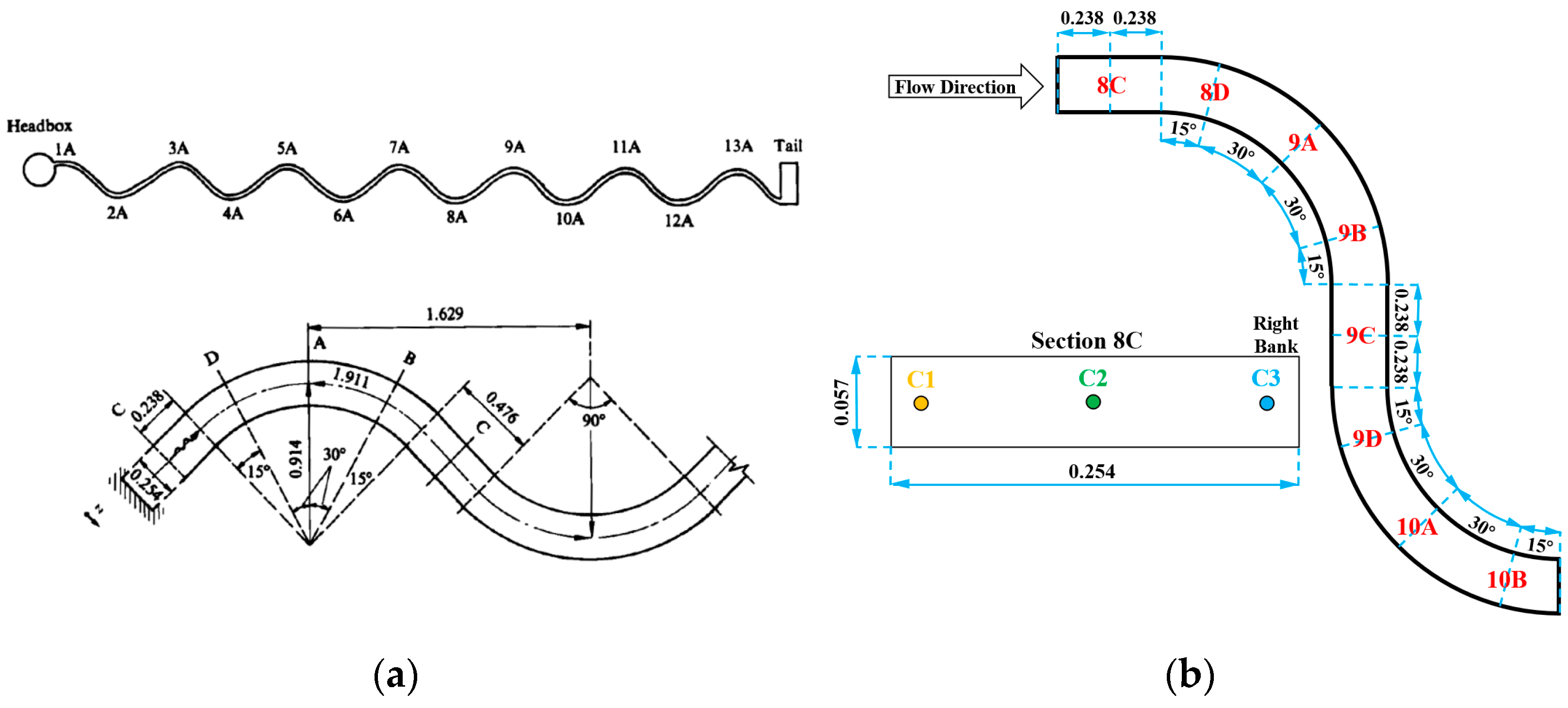
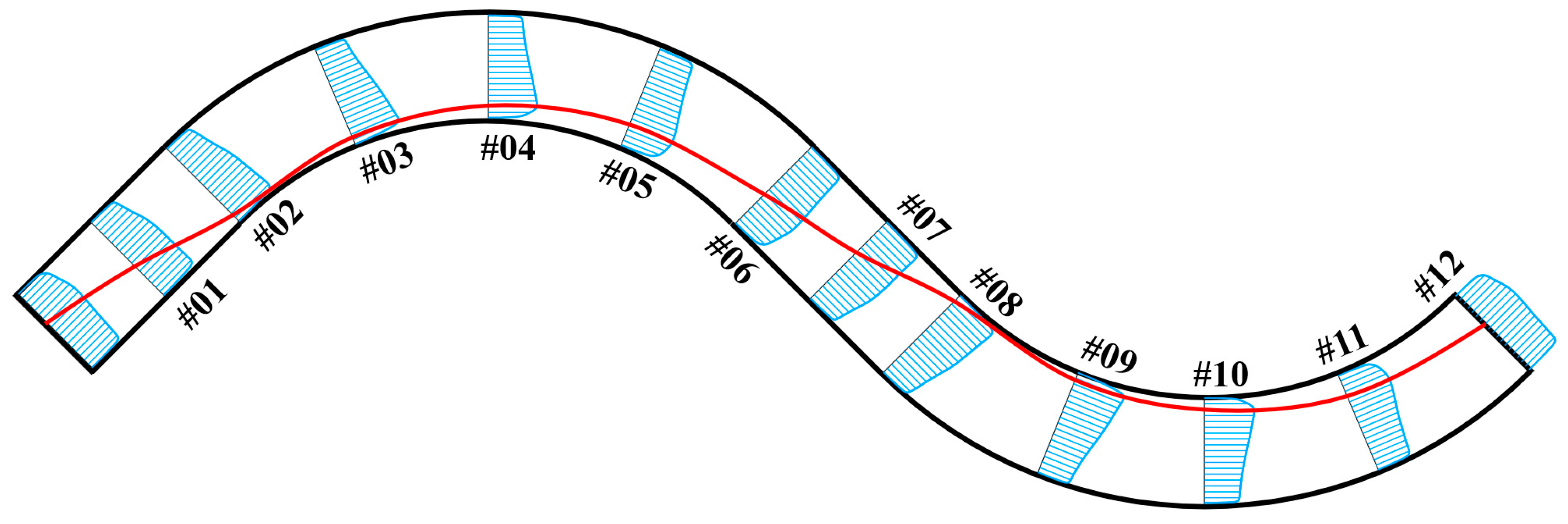
The flow measurements and tracer tests in meandering channels for model validation by the present work were conducted by Chang [5] in the Iowa Institute of Hydraulic Research. The schematic sketch and general view of the flume are shown in Figure 1. The experimental flume consists of 13 identical quadrants with a curvature radius of 0.914 m in alternating directions linked by straight reaches of 0.476 m in length. Two adjacent quadrants compose an S-shaped meander and the whole flume has seven consecutive meanders, with a total length of 25.91 m measured along the centerline of the channel. The width (W) and water depth (H) of the rectangular cross-section are 0.254 m and 0.057 m, respectively, and a bottom slope of 0.0012 was configured to obtain the desired flow condition. Other hydraulic parameters are shown in Table 1. The surface of the flume was covered by an epoxy-based paint, which can be treated as hydraulically smooth walls. A standard Prandtl-type pitot tube was utilized for velocity measurements.
The dispersant used for Chang’s experiment was a mixture of salt and methanol, the density of which is close to water and can act as a neutrally buoyant tracer (passive scalar). By controlling the discharge from the container, the tracer was injected from a 3.175 mm brass tube at a constant rate, whose effluent velocity was regulated to equal the ambient water velocity. The injections were located at the entrance of the 8th bend (Section 8C in Figure 1b), where the current reached a fully developed turbulent channel flow. Specifically, the injections were arranged at three different positions in the mid-depth, namely the left bank (C1), middle line (C2), and right bank (C3); the C1 and C3 were 0.0254 m away from the respective wall. To acquire detailed data of the tracer distribution, a computerized concentration measuring system was developed by interfacing a conductometer with an IBM 1801 Data Acquisition and Control System.
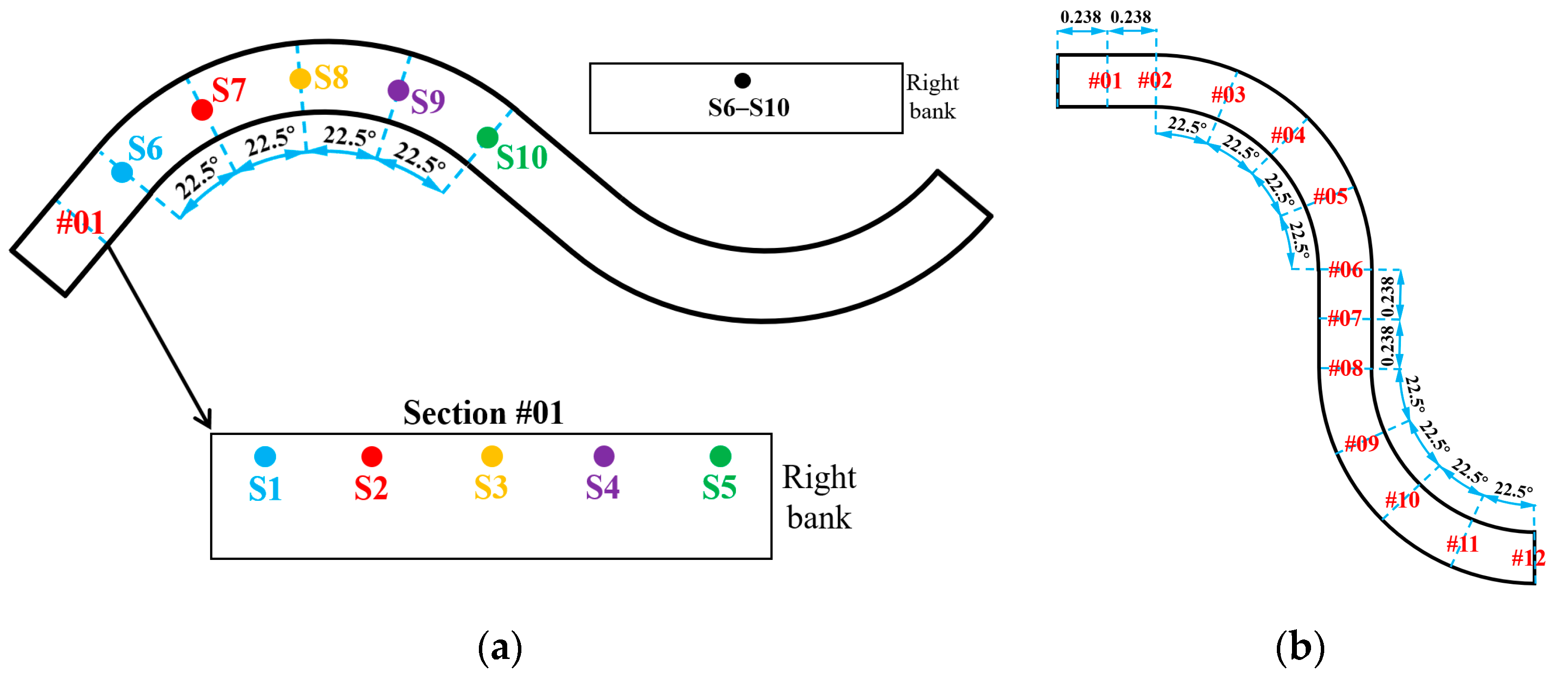
Numerical models with the same configuration as the experiments were established for model validation. Based on the verified model, additional computations were carried out to evaluate how different positions of continuous point source affects scalar’s distribution and mixing process. To achieve this goal, altogether 10 scenarios were set up, which are shown in Figure 2. The S1–S5 set were designed to compare the differences in transverse release points of scalar, while the S6–S10 set were designed to compare the differences in streamwise release points of scalar. For all the scenarios, the point sources were placed at the height of 0.0513 m (0.9 H) near the water surface. The S1 and S5 were 0.0254 m (0.1 W) away from the respective wall whereas the S2 and S4 were 0.0762 m (0.3 W) away from the corresponding wall. The S3 was in the centerline position and the S1–S5 were evenly distributed in transverse. For S6–S10, the point sources were all placed in the first half the meander at centerline of the channel. Furthermore, S6–S10 were arranged at identical intervals of 22.5 degrees from the entrance to the exit of the first bend.
For a comprehensive analysis of the result, Section #01–#12 in the meander were specified as a reference to better display the flow condition and scalar distribution along the channel.
2.3. Computational Domain and Boundary Conditions
Since the sinuous open channel has a periodic geometry on the plane, to save the computational cost, only one meander part was extracted from the entire sinuous channel. By establishing a periodic numerical model and running the simulation for some time, the flow condition and tracer transport process in the experiment can be well-reproduced.
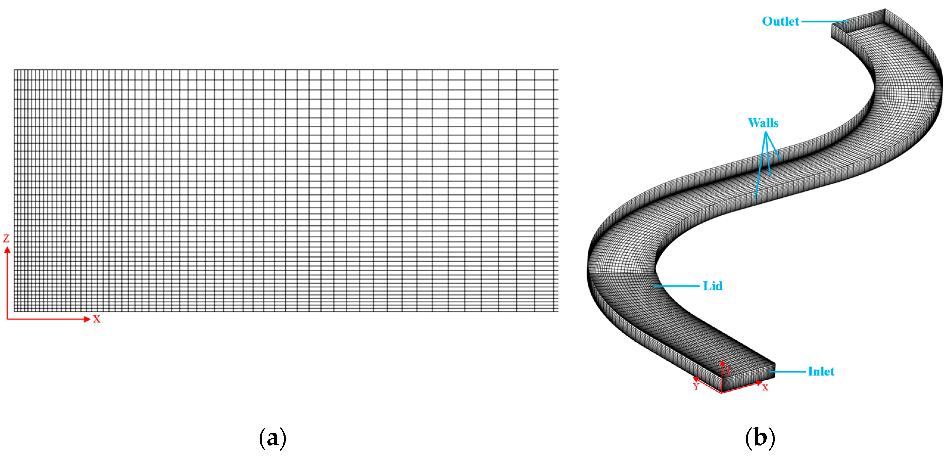
In the numerical model, a cartesian coordinate was used during the calculation, while for the data processing and analysis, the quantities were transformed into a cylindrical coordinate; the x-, y-, and z- axis hereby point to the transverse, streamwise, and vertical directions. The computational domain consists of 440 × 120 × 40 = 2.112 million structured grids in longitudinal, transverse, and vertical directions, respectively. The grid is uniform in streamwise and stretched in transverse and vertical direction to satisfy the requirement of the wall model. The expansion ratio is kept at a fixed value of 1.02 and the cell sizes in terms of wall units are y+ = z+ ≈ 12 close to walls. The sketch of grid cells is presented in Figure 3. For the sake of clarity, only left half of the cross-section is displayed (Figure 3a) and the grid line is partly shown in the domain (Figure 3b). The resolution of the grid is checked by a grid independence test based on comparisons (Figure 4) of three sets of grids (Table 2).
The size of a cell varies with its position within the profiles. To ensure the point sources among different cases are of the same volume, several cells were integrated as the domain where the source term works, with a nearly identical total volume as the experimental set up.
The domain of the numerical model includes four boundaries, namely, the Inlet, Outlet, Lid, and Walls as shown in Figure 3b. The periodic boundary condition is specified on the Inlet and Outlet. The boundary condition defined at the top boundary is the symmetry boundary condition which acts as a rigid lid. At Walls, the no-slip boundary condition for velocity and the Neumann boundary condition for pressure as well as scalar fields are employed. The nutUSpaldingWallFunction, a built-in wall model of OpenFOAM is imposed for subgrid-scale viscosity, eliminating the necessity of generating very fine mesh near solid boundaries. A tool in OpenFOAM called scalarFixedValueConstraint was used to set the scalar value to 0 in the upstream area close to the point source, which can constrain the pollutant in a single period. The flow is driven by configuring an additional body force pointing to the downslope direction.
All the simulations were performed for more than 50 large-eddy turnover times (channel length/bulk velocity) to reach a statistically stationary state. Additionally, 30 turnover times were then used to sample time-averaged data. The total simulation time was approximately 480 CPU hours with 96 cores (CPU: Intel Xeon 6240R, 48 cores per node).
3. Results and Discussion
In this section, the time-averaged values are denoted by the capital letters, whereas the instantaneous values are represented by the lower-case letters. For the convenience of data analysis, the velocity and scalar field were normalized by bulk velocity (Uav) and cross-sectional concentration (Cav), respectively. The variable names in the results are consistent with the following formula: Uh* = Uh/Uav (Uh is the depth-averaged streamwise velocity), U* = U/Uav, C* = C/Cav, u* = u/Uav, c* = c/Cav, CRMS* = CRMS/Cav. Moreover, the coordinate was scaled by the water depth (H) for brevity. Namely, X* = X/H, Y* = Y/H, Z* = Z/H.
3.1. Verification of Numerical Model
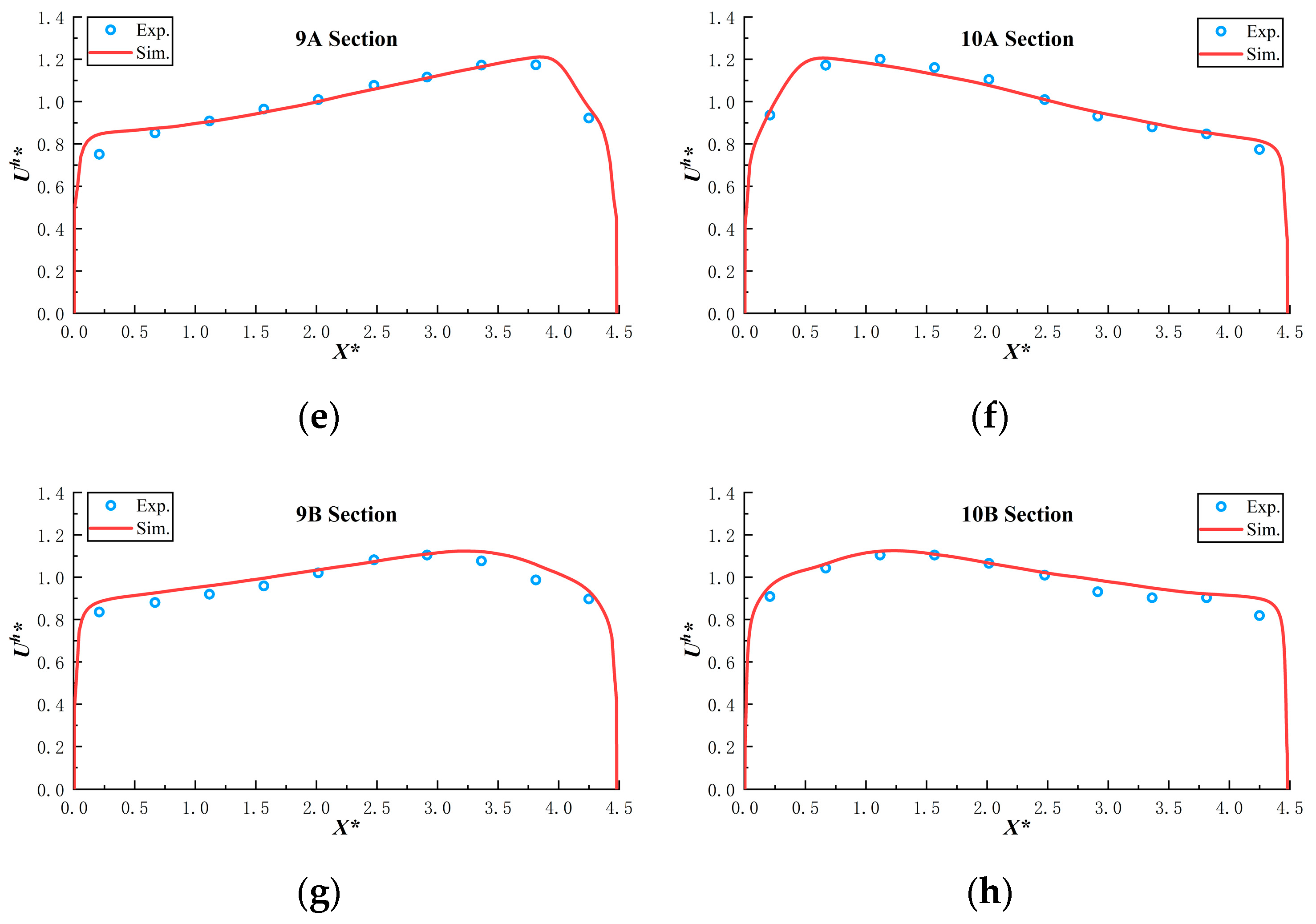
The depth-averaged streamwise velocity and concentration of the scalar from the simulation and experiment are compared for model validation. The measured and simulated dimensionless depth-averaged streamwise velocity Uh* is displayed in Figure 5. The comparison shows a similar trend between the two, which means a good agreement is obtained. It is noticeable that the streamwise velocity distributions of the upstream half of the bend (left column of Figure 5) are symmetrical to their counterparts from the downstream half of the bend (right column of Figure 5).
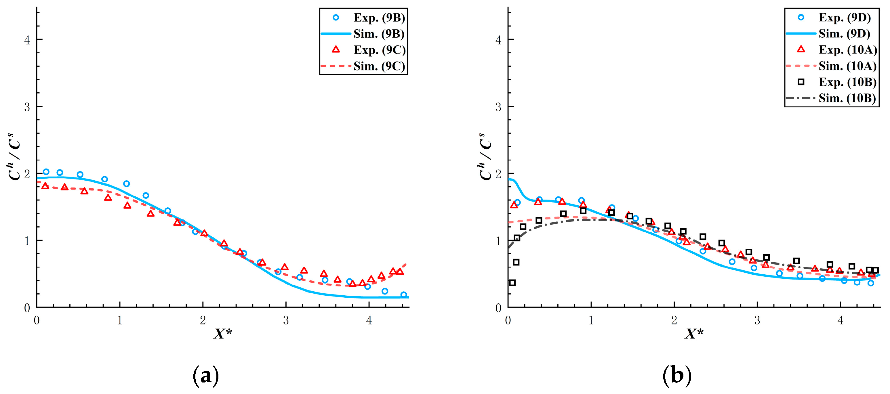
The measured and simulated depth-averaged scalar concentration Ch normalized by local mean concentration Cs is shown in Figure 6. The definition of local mean concentration Cs proposed by Chang [5] is:
where H is the water depth; Q is the discharge; Δx is the transverse length of sampling intervals; n is the number of sampling intervals.
The verification result of the scalar field is also satisfied with the similar trend between measurements and calculations. The peaks of transverse concentration distribution are almost at the same locations within the cross-sections, and the tiny deviations in some regions are acceptable. It is obvious that the transverse distribution of the concentration is different among C1, C2, and C3, especially in 9B and 9C sections, which results from the distinct release positions.
3.2. Time-Averaged Hydrodynamic Characteristics
3.2.1. Distribution of Streamwise Velocity
The normalized streamwise velocity U* in the form of contours and isolines are displayed in Figure 7. Considering the symmetric characteristic of velocity field in sinuous channels, only the upstream half of the meander is shown, namely Section #01–#06, whereas the velocities in the downstream half of the meander can be deduced. It demonstrates that the high velocity region gradually approaches the inner bank before entering the bend (Figure 7a,b), and this region is close to the inner bank wall within the bend (Figure 7c,d). From Section #04 the maximum velocity region starts to shift towards the centerline of the channel and repeat the above procedures in the next bend. This phenomenon coincides with the findings in some literatures [16,27]. It can be found that a shear layer is formed between the high velocity region and inner bank walls, where a high longitudinal velocity gradient occurs. This region normally generates streamwise oriented vortices (SOV) due to the effect of shearing and leads to high intensities of turbulence [28].
The plane view of the U* distribution and dynamic axis of flow is shown in Figure 8. It can be observed that the maximum velocity stays close to the inner bank within bends and goes back to the centerline in straight reaches. Moreover, the dynamic axis is found to take the shortest path marching forward along the channel.
3.2.2. Secondary Flow Structures
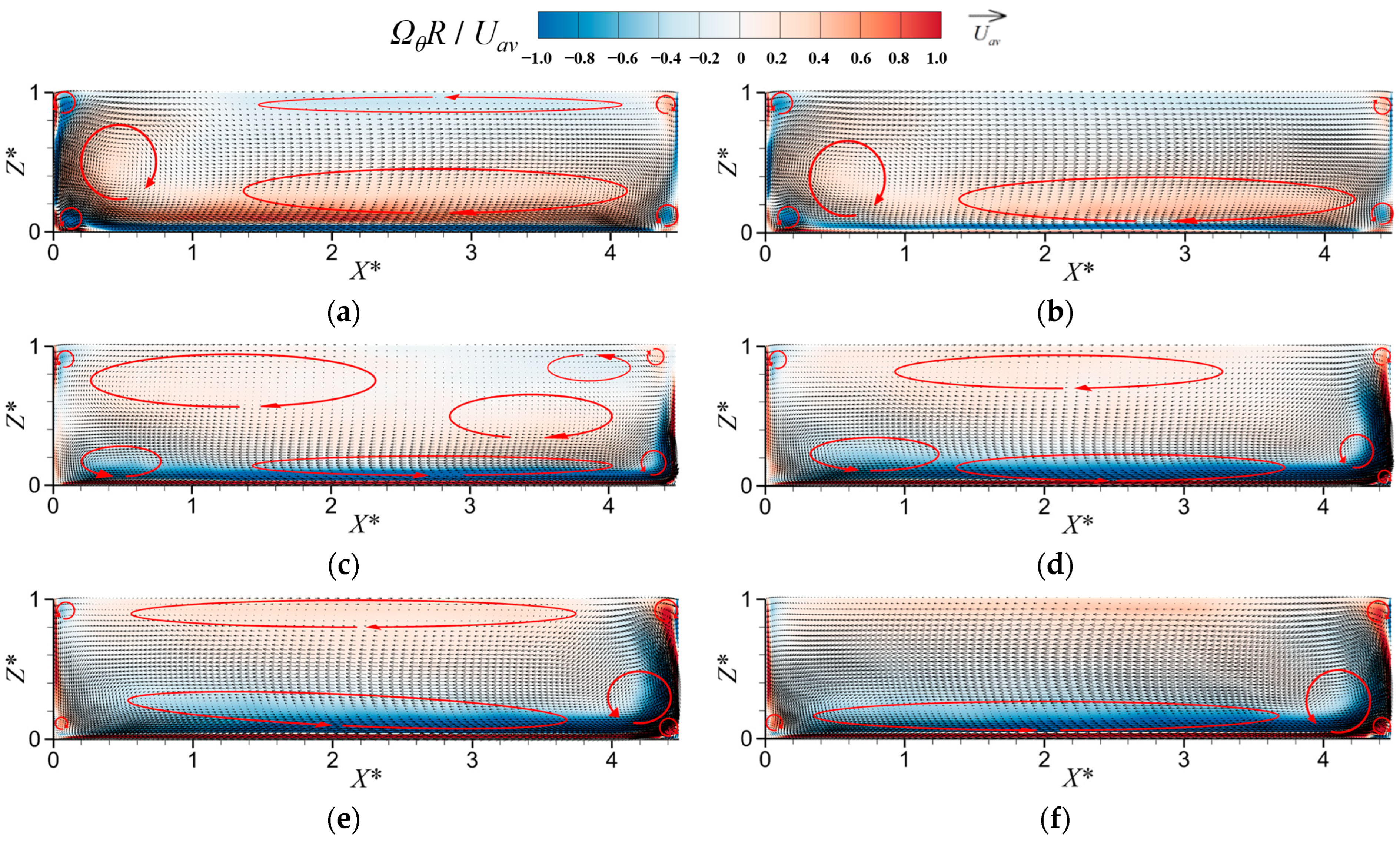
As stated before, secondary flow plays a significant role in the lateral mixing of the pollutant within meanders. To evaluate the effect of secondary current on pollutant transport, the vectors of secondary flow and contours of vorticities in typical cross-sections are presented in Figure 9. The vectors are non-dimensional with bulk velocity Uav, and the vorticities Ωθ are normalized through bulk velocity Uav and hydraulic radius R. As can be observed, there exists more than one large flow circulation in each section which are often called center-region cells [29]. Moreover, a flat circulation cell near the bottom that spans more than half of the section can be noticed, with an opposite rotational direction to that of cells located in the middle and upper part of the section. Moreover, at the four corners of a cross-section, small cells with different intensities are formed. Compared with the longitudinal velocity in Figure 7, it can be found that the value of vorticity in the region of high velocity is small, while the high vorticity occurs in the area with lower velocity near the sidewalls. It is clearly visible that near the bottom of the inner bank of Section #03–#06 (Figure 9c–f), a high intensity of vorticity is formed which was accompanied by a large velocity gradient and strong turbulence effect.
3.2.3. Turbulent Viscosity
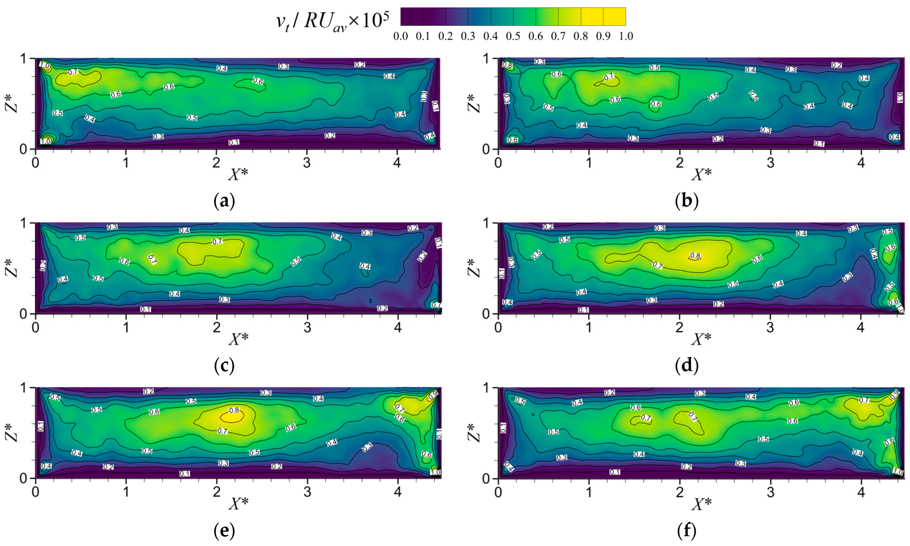
Turbulent viscosity dominates the diffusion rate in the process of pollutant mixing in turbulent flows. Figure 10 displays the distribution of normalized turbulent viscosity νt, and it reveals that the large turbulent viscosity mainly occurs in the region where the gradient of streamwise velocity is high (Figure 7). This phenomenon can also be deduced from Equations (6) and (8) that turbulent viscosity (subgrid viscosity) is proportional to the velocity gradient. In other words, the high gradient of streamwise velocity arising from flow shearing results in larger turbulent viscosity and vigorous diffusion. However, the secondary current is not the case (Figure 8), probably because its order of magnitude is smaller than that of streamwise velocity. The Van Driest damping function is employed so that the turbulent viscosity is relevantly low near walls despite a strong shear effect.
3.3. Time-Averaged Scalar Distribution
3.3.1. Time-Averaged Concentration Field
The simulation results reveal that the different release positions of pollutants from point sources significantly affect the downstream concentration distribution along the sinuous channel. Figure 11 displays the contours of the time-averaged concentration C* of S1, S3, and S5. It can be discovered that there are obvious differences in the variation in the pollutant concentration along the channel among the three scenarios. In S1 for example, the pollutants quickly reach the bottom and continue to transport to the right bank after release. However, there exists an evident difference in the speed of lateral spreading between the pollutants in the top and bottom part of the cross-section. At Section #05, the bottom pollutants reach the opposite bank and move upwards along the right bank until Section #07, where the high concentration region of the bottom contacts with that of the top, forming a concentric ring structure surrounding the water with low concentration. In S3, the pollutants are continuously transported to both the sides and bottom after release, presenting a radial shape. At Section #04, the center of the contaminant cloud moves to the bottom, and gradually deviates to the bottom of the left bank in the subsequent transport process, and a low concentration area appears at the top of the right bank. The contaminant cloud in S5 also quickly reaches the bottom, while the pollutants at the top continue to move to the left bank while the bottom is gradually penetrated by the water with low concentration from the left bank, and the center of the contaminant cloud gradually moves to the center of the section to form a concentric ring structure surrounding the high concentration pollutants. In comparison, the contaminant cloud in S1 and S3 eventually forms a belt concentrated at the bottom of the left bank, while S5 forms a contaminant cloud located in the center of the section. In addition, the maximum concentration of S3 is low, which indicates rapid mixing.
Compared with the flow structures in Figure 9, it can be found that the transverse transport process of pollutants in distinct scenarios is closely related to the secondary circulation. There exists a large range of flow motions from the left bank to the right bank in the middle and upper part of Section #02, which keep decreasing in the subsequent sections until it vanishes in Section #06. Meanwhile, a small range of flow motion can be observed from the right bank to the left bank near the bottom of Section #02, which continues to expand in the subsequent section until it almost occupies the whole section at Section #06. In addition, in Section #03 and the following sections, a flow motion from the left bank to the right bank at the bottom is generated. The above phenomenon of lateral flow motion leads to the differences in the pollutant transport process at the surface and bottom of the cross-section. It is worth noting that there is a small annular flow structure at the top corner of the section, which is an important incentive of faster vertical transport in S1 and S5. In addition, there is a strong turbulence structure at the bottom of the right bank within Section #04 to #06, but the mixing here is not significant.
3.3.2. Time-Averaged Concentration Flux
An effective method of analyzing the transport process of pollutants is the calculation of time-averaged concentration flux which represents the overall scalar transport rate. Figure 12 and Figure 13 show the cross-sectional averaged flux of concentration along the channel in the streamwise (Fs) and transverse direction (Ft), respectively. Fs and are Ft are calculated by the following equations:
where U and V denotes the time-averaged streamwise and transverse velocity, respectively; n is the number of sampling points within the profiles. The sampling points are uniformly distributed on the whole profiles whose data are obtained by performing interpolations from the data in the cell centers.
In Figure 12, the value of Fs shows obvious deviations in the vicinity of release points, which arises from the gathered contaminant cloud with high concentration. The curves gradually converge and maintain the trend until the end of the domain for S1–S5, which indicates that complete mixing is achieved. However, for S6–S10 the Fs rebound near the end of the domain, which may result from a significant difference in longitudinal velocity because the pollutants in S6–S10 are released in different positions in a streamwise direction. In Figure 13, the Ft in S1–S5 fluctuate along channel, presenting a nearly identical shape. These curve fluctuations result from the distinct strength of secondary circulation in different cross-sections. Stronger secondary motion leads to higher Ft. Meanwhile, the Ft in S6-S10 also fluctuates but with a shift between cases which also stems from the differences in streamwise release positions.
3.4. Instantaneous Field
The instantaneous flow characteristics and turbulence statistics of the concentration is analyzed in this section. The non-dimensional instantaneous quantities of streamwise velocity u* isolines (Figure 14), secondary current vectors as well as vorticity ωθ contours (Figure 15) and concentration distribution contours of S1, S3, and S5 (Figure 16) are displayed. For simplicity, only the slices of Section #04 and #07 were extracted, which are at the apex of the bend and the halfway point of the straight reach, respectively. Generally, the flow structure and concentration distribution are more disorganized and unstructured compared with time-averaged quantities. However, the high velocity region near the inner bank and a relevantly uniform velocity distribution in the straight channel, despite of the turbulence, can be observed. Moreover, the vectors of large-scale secondary motions are of similar directions and orders with time-averaged results. For the concentration field, the shapes of pollutant clouds of instantaneous values differ with that of time-averaged values, with a high spatial variability. Among three scenarios, S3 shows a higher mixing rate than the other two.
The root mean square fluctuations of concentration of S3 is shown in Figure 17. As can be seen in the contours, the intensities of the concentration fluctuations are of the same order of magnitude with the time-averaged quantities. The concentration fluctuations are mainly found in the vicinity of the release position of the point source, which is in accordance with other research [30,31,32]. The fluctuation plume significantly declines once it enters the straight reach (Figure 17e), while the concentration itself is relevantly high.
3.5. Mixing Efficiency
In order to evaluate the mixing efficiency of pollutant, two indices were imposed for the assessment of mixing rate along the channel. The normalized root mean square of concentration Cm within the profile is an effective parameter to quantify the uniformity of the pollutant’s spatial distribution, which have been widely used in similar studies [33,34]. The definition of Cm can be expressed by:
where Cav is the cross-sectional average concentration; Ci is the concentration of sampling points whose data are obtained by performing interpolations from the data in the cell centers. A smaller vale of Cm represents better mixing. Figure 18 demonstrates the variations in Cm of different scenarios along the channel. The curves of S1–S5 reveal a similar trend that the quantities all decrease sharply in the upstream half of the meander (region in Section #02–#06 marked on the Figure 18a), and then come to a slow decline in the straight reach. In the downstream half of the meander (region in Section #08–#12 marked on the Figure 18a) the curves gradually approach the horizontal axis and converge, which indicates that a good mixing was achieved among all the cases in this area; this is the case for S6–S10 in Figure 18b. However, some deviations can be observed in the upstream half of the meander where the values of Cm in S5 (Figure 18a) and S10 (Figure 18b) which are higher than the other cases, while the value of Cm in S3 and S4 as well as S8 and S9 is smaller in the rest of the region. This implies that both cases obtain a higher mixing rate under the effect of secondary flow in the upstream half of the meander. It can be concluded from variations in Cm that it is more likely to obtain a higher mixing rate when the point source is placed near the centerline in transverse and near the apex of the bend in streamwise. Furthermore, the mixing is mostly achieved in the first half of the meander period, while the mixing rate scarcely changes in the second half for all cases.
Another parameter proposed by Fischer [35] is the percentage of complete mixing P. It is generally considered that complete mixing is achieved if the concentration variations within a cross-section are ±5% of the downstream uniform concentration. P is then calculated through the ratio of complete mixing area to the whole cross-sectional area. Normally, a larger P represents a higher level of mixing. Figure 19 demonstrates the varying P of different scenarios along the channel. The curve demonstrates a clear distinction among cases along the channel. The S4 in Figure 19a and S8 along with S9 in Figure 19b present a higher level of mixing, which is in accordance with the conclusion drawn from Cm.
The Cm and P curves present a similar trend and have minor differences in each case group. To further quantitatively distinguish the overall mixing efficiency in the computational domain among different cases, the mean value Cm* and P* were calculated by averaging the Cm and P of all cross-sections in each case. Figure 20 displays the value of Cm* and P*, whereas the abscissa W stands for the point source’s distance from the left bank in S1–S5, and the abscissa Lb refers to the point source’s distance from the entrance of the bend in S6–S10. Generally, the point sources arranged near the centerline of the channel in transverse or near the apex of the bend in streamwise have relevantly lower Cm* and higher P*, which indicates a higher mixing rate. Specifically, the minimum value of Cm* is found in S3 (Figure 20a) and S8 (Figure 20b) of each set of cases, with a value of 0.334 and 0.218, respectively. However, the maximum value of P* is identified in S4 (Figure 20a) and S10 (Figure 20b), with a value of 0.228 and 0.295, respectively. This inconsistency indicates the contradiction between the two indices in picking the best-mixed scenario. As a result, an effective assessment of the pollutant’s mixing efficiency requires comprehensive consideration [36] with more than one index.
4. Conclusions
A three-dimensional large-eddy simulation model was established to investigate the influence of point source release positions on the pollutant mixing in sinuous open channel flows. The model was verified with a flume experiment involving tracer tests and the simulated results show good agreement to the measurements. Two sets of cases were specified, in which the point sources were placed at certain intervals in the spanwise and streamwise direction of the channel. By analyzing the flow features and comparing the characteristics of concentration distribution, the following conclusions can be drawn,
- The Smagorinsky model of LES is capable of reproducing the experimental data and capturing flow characteristics. Due to the geometry features, the hydrodynamics in the upstream half of the meander are symmetrical to their counterparts from the downstream half of the meander;
- The high streamwise velocity region keeps close to the inner bank wall within the bend. There exists a large gradient of streamwise velocity near the inner bank at the bend apex, where the streamwise oriented vortices (SOV) is generated. More than one center-region cell can be observed in each cross-section, along with small cells at section corners. The regions with high gradient of streamwise velocity are accompanied by large turbulent viscosity;
- Compared with the turbulent diffusion, large-scale secondary circulation plays a dominant role in the transport and mixing of pollutants. The spanwise flows near the top and bottom of the cross-sections significantly intensify the transverse transport of pollutants. The small cells at four section corners accelerate the vertical transport of pollutants, while the shear layer near the inner bank at the bend apex exerts little influence on the mixing;
- Different point source release positions result in a distinct transport process of pollutant in the downstream, and thus the mixing efficiency is influenced. Based on a qualitative analysis of the mean value of the RMS concentration Cm* and the percentage of complete mixing P* for the simulation cases, the mixing can be enhanced when the point sources are arranged near the centerline of the channel when Cm* = 0.334 and P* = 0.228, respectively, or near the apex of the bend when Cm* = 0.218 and P* = 0.295, respectively;
- Different indices of mixing degree can lead to different conclusions in determining the best-mixed scenario. Future study should be focused on the choice of the appropriate indices and the comprehensive consideration for the assessment of the mixing efficiency. The influence of the curvature of the bend or the different types of cross-sections on pollutant mixing should also be studied in the future.
Author Contributions
Conceptualization, H.Z. and S.L.; software, S.L.; validation, S.L., J.X. and S.Y.; formal analysis, H.Z. and S.L.; writing—original draft preparation, S.L.; writing—review and editing, H.Z.; data curation, H.Z. and S.L.; visualization, S.L. and J.X.; supervision, H.Z. and L.W.; funding acquisition H.Z. and L.W. All authors have read and agreed to the published version of the manuscript.
Funding
This research was funded by the National Key R&D Program of China (Grant No. 2021YFC3200403), the National Natural Science Foundation of China (Grant No. 51879086), the Fundamental Research Funds for the Central Universities (Grant No. B200204044) and the Research Funding of China Three Gorges Corporation (Grant No. 202003251).
Institutional Review Board Statement
Not applicable.
Informed Consent Statement
Not applicable.
Data Availability Statement
Not applicable.
Acknowledgments
The numerical calculation was conducted on the clusters of HPC platform in Hohai University. Moreover, the author would like to thank anyone who contributes to the construction of the OpenFOAM community.
Conflicts of Interest
The authors declare no conflict of interest.
References
- Blanckaert, K.; Graf, W.H. Momentum transport in sharp open-channel bends. J. Hydraul. Eng. 2004, 130, 186–198. [Google Scholar] [CrossRef]
- Blanckaert, K. Hydrodynamic processes in sharp meander bends and their morphological implications. J. Geophys. Res. Earth Surf. 2011, 116, F01003. [Google Scholar] [CrossRef] [Green Version]
- Fischer, H.B. The effect of bends on dispersion in streams. Water Resour. Res. 1969, 5, 496–506. [Google Scholar] [CrossRef]
- Boxall, J.B. Dispersion of Solutes in Sinuous Open Channel Flows; University of Sheffield: Sheffield, UK, 2000. [Google Scholar]
- Chang, Y.C. Lateral Mixing in Meandering Channels; University of Iowa: Iowa City, IA, USA, 1971. [Google Scholar]
- Fukuoka, S. Longitudinal Dispersion in Sinuous Channels; University of Iowa: Iowa City, IA, USA, 1971. [Google Scholar]
- Boxall, J.B.; Guymer, I. Analysis and Prediction of Transverse Mixing Coefficients in Natural Channels. J. Hydraul. Eng. 2003, 129, 129–139. [Google Scholar] [CrossRef]
- Shaheed, R.; Mohammadian, A.; Yan, X. A Review of Numerical Simulations of Secondary Flows in River Bends. Water 2021, 13, 884. [Google Scholar] [CrossRef]
- Duan, J.G. Simulation of Flow and Mass Dispersion in Meandering Channels. J. Hydraul. Eng. 2004, 130, 964–976. [Google Scholar] [CrossRef]
- Demuren, A.O.; Rodi, W. Calculation of flow and pollutant dispersion in meandering channels. J. Fluid Mech. 1986, 172, 63–92. [Google Scholar] [CrossRef]
- Huang, H.; Chen, G.; Zhang, Q. Influence of River Sinuosity on the Distribution of Conservative Pollutants. J. Hydrol. Eng. 2012, 17, 1296–1301. [Google Scholar] [CrossRef]
- Huang, H.; Chen, G.; Zhang, Q. The distribution characteristics of pollutants released at different cross-sectional positions of a river. Environ. Pollut. 2010, 158, 1327–1333. [Google Scholar] [CrossRef]
- Booij, R. Measurements and large eddy simulations of the flows in some curved flumes. J. Turbul. 2003, 4, N8. [Google Scholar] [CrossRef]
- Stoesser, T.; Ruether, N.; Olsen, N.R.B. Calculation of primary and secondary flow and boundary shear stresses in a meandering channel. Adv. Water Resour. 2010, 33, 158–170. [Google Scholar] [CrossRef]
- Van Balen, W.; Blanckaert, K.; Uijttewaal, W.S.J. Analysis of the role of turbulence in curved open-channel flow at different water depths by means of experiments, LES and RANS. J. Turbul. 2010, 11, N12. [Google Scholar] [CrossRef]
- Moncho-Esteve, I.J.; Folke, F.; García-Villalba, M.; Palau-Salvador, G. Influence of the secondary motions on pollutant mixing in a meandering open channel flow. Environ. Fluid Mech. 2017, 17, 695–714. [Google Scholar] [CrossRef]
- Balen, B.V.; Uijtewall, W.; Blanckaert, K. Scalar Dispersion in Strongly Curved Open-Channel Flows; Bundesanstalt für Wasserbau: Karlsruhe, Germany, 2010. [Google Scholar]
- Zhu, H.; Lin, C.; Wang, L.; Kao, M.; Tang, H.; Williams, J.J. Numerical investigation of internal solitary waves of elevation type propagating on a uniform slope. Phys. Fluids 2018, 30, 116602. [Google Scholar] [CrossRef]
- Palau-Salvador, G.; Garcı’a-Villalba, M.; Rodi, W. Scalar transport from point sources in the flow around a finite-height cylinder. Environ. Fluid Mech. 2011, 11, 611–625. [Google Scholar] [CrossRef]
- Zhang, B.; Dong, X.; Ji, C. Large eddy simulations of hydrodynamic structure in channel bends with large width-depth ratios and variable curvatures (in Chinese). J. Hydroelectr. Eng. 2019, 38, 77–91. [Google Scholar]
- Van Balen, W.; Uijttewaal, W.S.J.; Blanckaert, K. Large-eddy simulation of a mildly curved open-channel flow. J. Fluid Mech. 2009, 630, 413–442. [Google Scholar] [CrossRef] [Green Version]
- Dong, X.; Bai, Y.; Munjiza, A. Investigation on the Characteristics of Turbulent Flow in a Meandering Open Channel Bend Using Large Eddy Simulation. In Proceedings of the 35th IAHR World Congress, Chengdu, China, 8–13 September 2013. [Google Scholar]
- Versteeg, H.K.; Malalasekera, W. An Introduction to Computational Fluid Dynamics: The Finite Volume Method; Pearson Education: London, UK, 2007. [Google Scholar]
- Greenshields, C.J. OpenFOAM User Guide Version 7; The OpenFOAM Foundation: London, UK, 2018; p. 237. [Google Scholar]
- Liu, F. A Thorough Description of How Wall Functions Are Implemented in OpenFOAM. In Proceedings of the CFD with OpenSource Software, Gothenburg, Sweden, 12–14 December 2016; Nilsson, H., Ed.; [Google Scholar]
- Jasak, H. Error Analysis Estimation for the Finite Volume Method with Applications to Fluid Flows; The Imperial College of Science, Technology and Medicine: London, UK, 1996. [Google Scholar]
- Blanckaert, K.; Graf, W.H. Mean flow and turbulence in open-channel bend. J. Hydraul. Eng. 2001, 127, 835–847. [Google Scholar] [CrossRef]
- Koken, M.; Constantinescu, G.; Blanckaert, K. Hydrodynamic processes, sediment erosion mechanisms, and Reynolds-number-induced scale effects in an open channel bend of strong curvature with flat bathymetry. J. Geophys. Res. Earth Surf. 2013, 118, 2308–2324. [Google Scholar] [CrossRef]
- Blanckaert, K.; De Vriend, H.J. Secondary flow in sharp open-channel bends. J. Fluid Mech. 2004, 498, 353–380. [Google Scholar] [CrossRef] [Green Version]
- Wagner, C.; Kuhn, S.; Rohr, P.R. Scalar transport from a point source in flows over wavy walls. Exp. Fluids 2007, 43, 261–271. [Google Scholar] [CrossRef] [Green Version]
- Shiono, K.; Feng, T. Turbulence measurements of dye concentration and effects of secondary flow on distribution in open channel flows. J. Hydr. Eng. 2001, 129, 373–384. [Google Scholar] [CrossRef]
- Fackrell, J.E.; Robins, A.G. Concentration fluctuations and fluxes in plumes from point sources in a turbulent boundary layer. J. Fluid Mech. 1982, 117, 1–26. [Google Scholar] [CrossRef]
- Pouchoulin, S.; Mignot, E.; Rivière, N.; Le Coz, J. Numerical simulations on mixing of passive scalars in river confluences. E3S Web Conf. 2018, 40, 05019. [Google Scholar] [CrossRef]
- Denev, J.A.; Frohlich, J.; Bockhorn, H. Large eddy simulation of a swirling transverse jet into a crossflow with investigation of scalar transport. Phys. Fluids 2009, 21, 015101. [Google Scholar] [CrossRef]
- Fischer, H.B.; List, E.J.; Koh, R.C.Y.; Imberger, J.; Brooks, N.H. Mixing in Inland and Coastal Waters; Academic Press: Cambridge, MA, USA, 1979. [Google Scholar]
- Yuan, S.; Tang, H.; Li, K.; Xu, L.; Xiao, Y.; Gualtieri, C.; Rennie, C.; Melville, B. Hydrodynamics, sediment transport and morphological features at the confluence between the Yangtze River and the Poyang Lake. Water Resour. Res. 2021, 57. [Google Scholar] [CrossRef]
Figure 1.
Sketch of the flume (Dimensions in meter): (a) plane view (adapted from Chang [5]); (b) geometry of a meander and the release positions of point source tracer of C1, C2, and C3.
Figure 1.
Sketch of the flume (Dimensions in meter): (a) plane view (adapted from Chang [5]); (b) geometry of a meander and the release positions of point source tracer of C1, C2, and C3.

Figure 2.
Information on the considered cases in numerical study: (a) the locations of point source in all scenarios; (b) typical cross-sections in the meander.
Figure 2.
Information on the considered cases in numerical study: (a) the locations of point source in all scenarios; (b) typical cross-sections in the meander.

Figure 3.
The sketch of mesh: (a) left half of cross-sectional grid line; (b) overview of the computational domain and boundaries (every 3rd grid line is displayed).
Figure 3.
The sketch of mesh: (a) left half of cross-sectional grid line; (b) overview of the computational domain and boundaries (every 3rd grid line is displayed).

Figure 4.
The grid independence test results: (a) normalized depth-averaged streamwise velocity Uh*; (b) normalized depth-averaged concentration Ch/Cs (defined in Section 3.1).
Figure 4.
The grid independence test results: (a) normalized depth-averaged streamwise velocity Uh*; (b) normalized depth-averaged concentration Ch/Cs (defined in Section 3.1).

Figure 5.
Comparison between simulations and measurements in dimensionless depth-averaged streamwise velocity Uh*: (a–h) 8C to 10B cross-section along the meander in the experiment.
Figure 5.
Comparison between simulations and measurements in dimensionless depth-averaged streamwise velocity Uh*: (a–h) 8C to 10B cross-section along the meander in the experiment.


Figure 6.
Comparison between simulations and measurements in depth-averaged concentration of the scalar Ch, made non-dimensional with local mean concentration Cs: (a,b) C1 scenario; (c,d) C2 scenario; (e,f) and C3 scenario.
Figure 6.
Comparison between simulations and measurements in depth-averaged concentration of the scalar Ch, made non-dimensional with local mean concentration Cs: (a,b) C1 scenario; (c,d) C2 scenario; (e,f) and C3 scenario.


Figure 7.
Normalized streamwise velocity U* (from left to right denotes from inner bank to outer bank). (a) Section #01; (b) Section #02; (c) Section #03; (d) Section #04; (e) Section #05; (f) and Section #06.
Figure 7.
Normalized streamwise velocity U* (from left to right denotes from inner bank to outer bank). (a) Section #01; (b) Section #02; (c) Section #03; (d) Section #04; (e) Section #05; (f) and Section #06.

Figure 8.
Depth-averaged streamwise velocity Uh* distribution along channel in typical cross-sections and the dynamic axis of flow (the solid curve inside the channel).
Figure 8.
Depth-averaged streamwise velocity Uh* distribution along channel in typical cross-sections and the dynamic axis of flow (the solid curve inside the channel).

Figure 9.
Normalized vectors of secondary currents velocities with a background of contours showing dimensionless streamwise vorticity. (From left to right denotes from inner bank to outer bank). (a) Section #01; (b) Section #02; (c) Section #03; (d) Section #04; (e) Section #05; (f) and Section #06.

Figure 10.
The contours and isolines of turbulent viscosity. (From left to right denotes from inner bank to outer bank). (a) Section#01; (b) Section#02; (c) Section#03; (d) Section#04; (e) Section#05; (f) and Section#06.
Figure 10.
The contours and isolines of turbulent viscosity. (From left to right denotes from inner bank to outer bank). (a) Section#01; (b) Section#02; (c) Section#03; (d) Section#04; (e) Section#05; (f) and Section#06.

Figure 11.
Non-dimensional scalar concentration C* in some typical profiles. (From left to right denotes from inner bank to outer bank). (a) Case S1; (b) Case S3; (c) and Case S5.
Figure 11.
Non-dimensional scalar concentration C* in some typical profiles. (From left to right denotes from inner bank to outer bank). (a) Case S1; (b) Case S3; (c) and Case S5.

Figure 12.
Cross-sectional averaged streamwise concentration flux along the channel. (a) Case S1–S5; (b) and Case S6–S10.
Figure 12.
Cross-sectional averaged streamwise concentration flux along the channel. (a) Case S1–S5; (b) and Case S6–S10.

Figure 13.
Cross-sectional averaged transverse flux of concentration along the channel. (a) Case S1–S5; (b) and Case S6–S10.
Figure 13.
Cross-sectional averaged transverse flux of concentration along the channel. (a) Case S1–S5; (b) and Case S6–S10.

Figure 14.
The normalized instantaneous streamwise velocity u*. (a) Section #04 in Case S1–S10; (b) and Section #07 in Case S1–S10.
Figure 14.
The normalized instantaneous streamwise velocity u*. (a) Section #04 in Case S1–S10; (b) and Section #07 in Case S1–S10.

Figure 15.
The normalized instantaneous velocity vectors and streamwise vorticity. (a) Section #04 in Case S1–S10; (b) and Section #07 in Case S1–S10.
Figure 15.
The normalized instantaneous velocity vectors and streamwise vorticity. (a) Section #04 in Case S1–S10; (b) and Section #07 in Case S1–S10.

Figure 16.
The normalized instantaneous concentration c*. (From left to right denotes from inner bank to outer bank). (a) Section #04 in Case S1; (b) Section #07 in Case S1; (c) Section #04 in Case S3; (d) Section #07 in Case S3; (e) Section #04 in Case S5; (f) and Section #07 in Case S5.
Figure 16.
The normalized instantaneous concentration c*. (From left to right denotes from inner bank to outer bank). (a) Section #04 in Case S1; (b) Section #07 in Case S1; (c) Section #04 in Case S3; (d) Section #07 in Case S3; (e) Section #04 in Case S5; (f) and Section #07 in Case S5.

Figure 17.
The dimensionless RMS fluctuations of concentration CRMS* in S3. (From left to right denotes from inner bank to outer bank). (a) Section #02 in Case S3; (b) Section #03 in Case S3; (c) Section #04 in Case S3; (d) Section #05 in Case S3; (e) Section #06 in Case S3; (f) and Section #07 in Case S3.

Figure 18.
Normalized root mean square of concentration Cm in different scenarios along the channel. (a) Case S1–S5; (b) and Case S6–S10.
Figure 18.
Normalized root mean square of concentration Cm in different scenarios along the channel. (a) Case S1–S5; (b) and Case S6–S10.

Figure 19.
Percentage of complete mixing P in different scenarios along the channel. (a) Case S1–S5; (b) and Case S6–S10.
Figure 19.
Percentage of complete mixing P in different scenarios along the channel. (a) Case S1–S5; (b) and Case S6–S10.

Figure 20.
The value of Cm* and P* in S1–S10. (a) Case S1–S5; (b) and Case S6–S10.


Table 1.
Hydraulic parameters of the experiment.
| Hydraulic Radius R (m) | Aspect Ratio | Bulk Velocity Uav (m/s) | Shear Velocity Us (m/s) | Friction Factor | Re (4UavR/ν) | Fr (Uav/√gH) |
|---|---|---|---|---|---|---|
| 0.039 | 4.47 | 0.354 | 0.0214 | 0.0293 | 40,000 | 0.473 |
Table 2.
Configurations of three sets of grids.
| Grid Number | Cell Numbers in: Streamwise × Transverse × Vertical | Total Cells (Million) | Δx+, Δz+ | Δy+ |
|---|---|---|---|---|
| #01 | 360 × 80 × 28 | 0.8064 | 18 | 150 |
| #02 | 440 × 120 × 40 | 2.112 | 12 | 120 |
| #03 | 550 × 180 × 60 | 5.94 | 8 | 96 |
Publisher’s Note: MDPI stays neutral with regard to jurisdictional claims in published maps and institutional affiliations. |
© 2022 by the authors. Licensee MDPI, Basel, Switzerland. This article is an open access article distributed under the terms and conditions of the Creative Commons Attribution (CC BY) license (https://creativecommons.org/licenses/by/4.0/).
Share and Cite
MDPI and ACS Style
Zhu, H.; Lu, S.; Wang, L.; Xu, J.; Yuan, S. Numerical Study of Mixing Process by Point Source Pollution with Different Release Positions in a Sinuous Open Channel. Water 2022, 14, 1903. https://doi.org/10.3390/w14121903
AMA Style
Zhu H, Lu S, Wang L, Xu J, Yuan S. Numerical Study of Mixing Process by Point Source Pollution with Different Release Positions in a Sinuous Open Channel. Water. 2022; 14(12):1903. https://doi.org/10.3390/w14121903
Chicago/Turabian StyleZhu, Hai, Shengjie Lu, Lingling Wang, Jieru Xu, and Saiyu Yuan. 2022. "Numerical Study of Mixing Process by Point Source Pollution with Different Release Positions in a Sinuous Open Channel" Water 14, no. 12: 1903. https://doi.org/10.3390/w14121903
Note that from the first issue of 2016, this journal uses article numbers instead of page numbers. See further details here.