
Application of Image Technique to Obtain Surface Velocity and Bed Elevation in Open-Channel Flow


Department of Civil Engineering, National Taiwan University, Taipei City 106, Taiwan
*
Author to whom correspondence should be addressed.
Water 2022, 14(12), 1895; https://doi.org/10.3390/w14121895
Submission received: 18 March 2022
/
Revised: 7 June 2022
/
Accepted: 10 June 2022
/
Published: 13 June 2022
(This article belongs to the Special Issue Advances in Experimental Hydraulics, Coast and Ocean Hydrodynamics)
Abstract
:The frequency of droughts and floods is increasing due to the extreme climate. Therefore, water resource planning, allocation, and disaster prevention have become increasingly important. One of the most important kinds of hydrological data in water resources planning and management is discharge. The general way to measure the water depth and discharge is to use the Acoustic Doppler Current Profiler (ADCP), a semi-intrusive instrument. This method would involve many human resources and pose severe hazards by floods and extreme events. In recent years, it has become mainstream to measure hydrological data with nonintrusive methods such as the Large-Scale Particle Image Velocimetry (LSPIV), which is used to measure the surface velocity of rivers and estimate the discharge. However, the unknown water depth is an obstacle for this technique. In this study, a method combined with LSPIV to estimate the bathymetry was proposed. The experiments combining the LSPIV technique and the continuity equation to obtain the bed elevation were conducted in a 27 m long and 1 m wide flume. The flow conditions in the experiments were ensured to be within uniform and subcritical flow, and thermoplastic rubber particles were used as the tracking particles for the velocity measurement. The two-dimensional bathymetry was estimated from the depth-averaged velocity and the continuity equation with the leapfrog scheme in a predefined grid under the constraints of Courant–Friedrichs–Lewy (CFL). The LSPIV results were verified using Acoustic Doppler Velocimetry (ADV) measurements, and the bed elevation data of this study were verified using conventional point gauge measurements. The results indicate that the proposed method effectively estimated the variation of the bed elevation, especially in the shallow water level, with an average accuracy of 90.8%. The experimental results also showed that it is feasible to combine the nonintrusive imaging technique with the numerical calculation in solving the water depth and bed elevation.
1. Introduction
Discharge is the fundamental parameter describing the flow characteristics of open channels, and is also an essential factor in designing water conservation structures, flood warning systems, and water resources planning and management [1,2]. The traditional flow monitoring method measures the discharge corresponding to the water level in different normal flow conditions, establishes a rating curve between the water level and discharge, and indirectly estimates the discharge by real-time water level measurement [3]. On the other hand, discharge measurements using the Acoustic Doppler Current Profiler (ADCP) are conducted by dividing the river cross-section into blocks. In each block, the water depth and average flow velocity or velocity array data is measured to obtain the discharge [4,5]. However, when extreme events occur, the flow measurements in high discharges are not enough for the rating curve approach. The measured curve in an extreme event can be extrapolated only for normal flow conditions [6,7]. Moreover, the operator is at considerable risk when the flood occurs, since the instrument is difficult to operate. Consequently, less data on the relationship between the water level and discharge in high discharge leads to the uncertainty of the measured discharge. In addition, the variation of the water depth in the measured section due to strong scouring and deposition takes time and effort to resurvey [8,9].
Applying nonintrusive methods, such as LSPIV [10], has become popular and widely used to measure hydrological data. Bradley [11] used LSPIV to calculate the discharge at stream cross-sections in Clear Creek, Iowa, generating an approximate 6.4% difference compared to the actual discharge data. Tekehara [12] conducted speed measurement with LSPIV and tracer particles made of biodegradable starch for the Uji River, Kizu River, and Katsura River in Japan on a helicopter. The results show an approximate error within one pixel. Meselhe [13] discussed the effectiveness and restraints of LSPIV in shallow flows with low velocity in the flume experiment, and found that the accuracy of LSPIV does not decrease even when the flow velocity is reduced to 0.015 m/s. As a result, the LSPIV is an appropriate technique for flow fields where the velocity is smaller than the limit of other measuring instruments. Dermisis and Papanicolaou [14] conducted velocity field in free surface with LSPIV around fish ladders and weirs, and compared the result with Acoustic Doppler Velocimetry (ADV), receiving an approximate error of 10%. Kim [15] listed out 27 sources of errors after analyzing the uncertainty of LSPIV. Among them, particle density, image shooting distance, and coordinate conversion were the three major sources that caused significant impact on the LSPIV measurement. In addition, with the rapid development of technology, LSPIV measurement technology has gradually been applied to unmanned aerial vehicles. This makes flow rate measurements in the field more flexible and faster. The measurement range also becomes more extensive [16,17]. In general, many studies have shown that LSPIV can measure flow velocities in the field and provide real-time digital measurements in a cost-effective manner [18,19,20,21].
Johnson and Cowen [22] used LSPIV to estimate the discharge by measuring the instantaneous surface velocities and establishing the relationship between the integrated length and water depth. The relationship between the integrated length and water depth can be established using a large amount of experimental data. However, the method encountered low resolution and inaccurate surface velocity for in situ measurements. To obtain the flow parameters with nonintrusive methods, this study aims to solve the continuity equation and invert the bottom bed elevation using the flow velocity measured by LSPIV as the boundary condition. The shallow water equation is a set of first-order nonlinear hyperbolic partial differential equations characterized by much larger horizontal and velocity scales than vertical scales, and the equation is effective in representing many physical phenomena in rivers and canals [23,24]: the flow pattern during a dam collapse [25,26], the simulation of soil flow around a catchment [27,28], and the calculation of tsunami wave transmission time [29,30]. However, since the shallow water equation is a nonlinear partial differential equation, it is difficult to obtain an analytical solution. Numerical approximation is then required to obtain an approximate solution. The concept of the leapfrog method was first applied to the shallow water equation by Mesinger and Arakawa in 1976 and effectively simulated real flow conditions [31]. Afterward, Zhou [32] modified the leapfrog method with the semi-implicit staggered time grid system, which turned out to double the computational efficiency. Nevertheless, the semi-implicit scheme for the modified leapfrog method can reduce the convergence of the equation. To design a numerical method that effectively simulate real flow conditions, Stelling and Duinmeijer [33,34] introduced the explicit staggered grid scheme for the leapfrog method for shallow water equations. The method can be applied in rapidly changing flow transition zones, such as hydraulic jumps.
To test the feasibility of obtaining underwater topographic variations by solving the continuity equation, a series of experiments were conducted in the flume with five different substrate beds under three different flow conditions. Additionally, the depth-averaged velocity can be calculated using a velocity coefficient k, defined as the depth-average velocity to surface velocity ratio. Generally, the value of k = 0.85 is accepted for river flows by the hydraulic community [35,36,37,38]. With the depth-averaged velocity and discretizing the derivatives of the continuity equation among the neighboring points in space with the leapfrog scheme, the approximate water depth at each grid point can be determined. Finally, the measured bed elevation is compared to the true value to evaluate the accuracy and feasibility of this proposed method.
2. Mathematical Formulation
2.1. LSPIV Algorithm
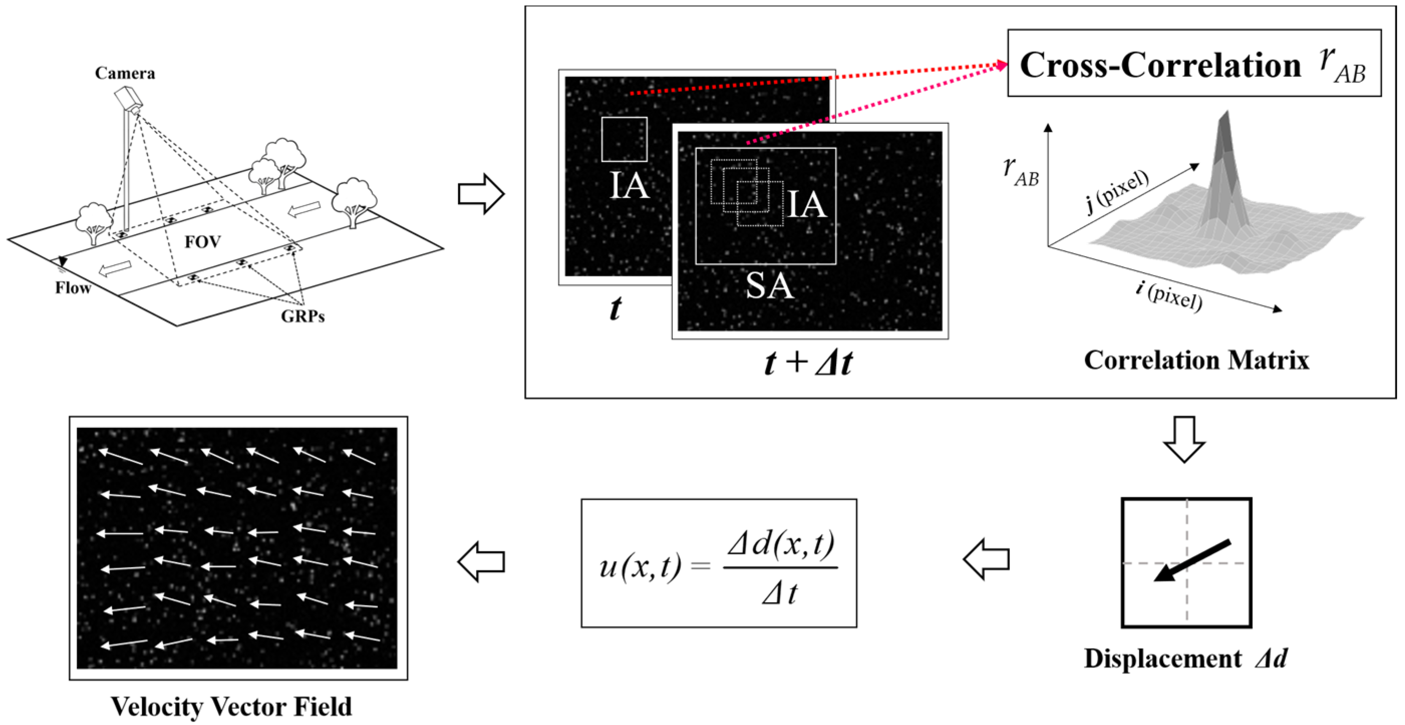
Large-Scale Particle Image Velocimetry (LSPIV) is a nonintrusive measurement that can obtain two-dimensional velocity fields (Figure 1) [39,40]. LSPIV measurements were performed using the consecutive images recorded by a fixed camera. Then, the surface velocity can be calculated by tracking the moving distance between the distinct pattern and the time difference in two consecutive images Equation (1).
The Direct Cross-Correlation (DCC) algorithm [41], an image-matching method in this study, is used to track features of surface seedings. In the algorithm, it requires to define a subimage called the Interrogation Area (IA) and delineate the Searching Area (SA). This enables the computer to find the most similar candidate subimages (as shown in Figure 1) in the image at and their moving distance. DCC is a method that calculates the cross-correlation between two matching IAs in space by the difference in brightness distribution. The cross-correlation is calculated as:
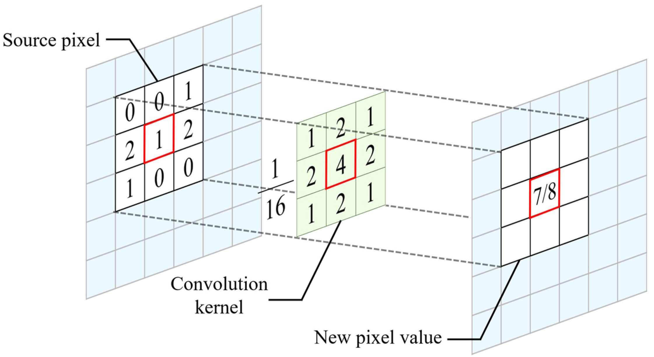
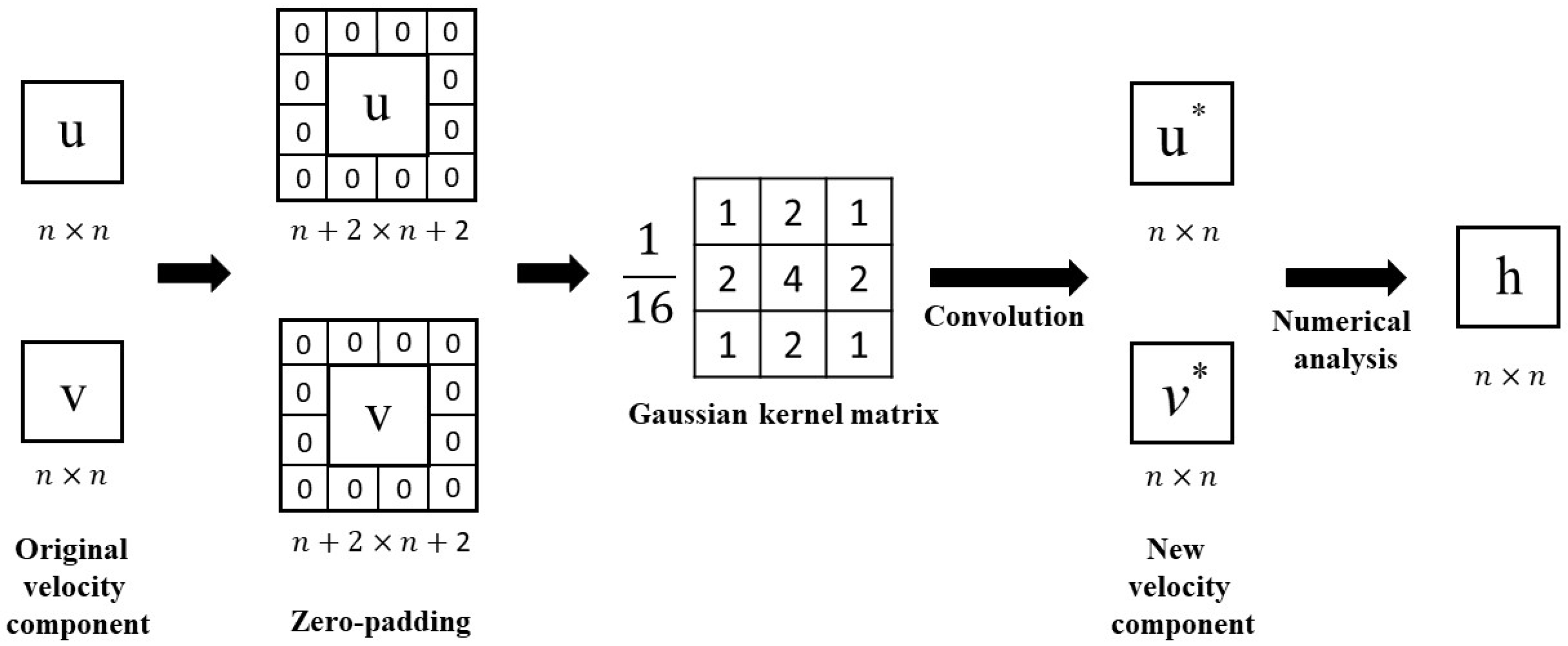
The distance the particle moves is calculated by the cross-correlation matrix obtained between subimage A at and each matching subimage B at . The peak value represents the location of the matching subimage B with the highest correlation with subimage A at , and the distance between A and B can be regarded as the displacement distance of the seeding movement. In addition, to reduce the excessive noise caused by the grid size of the two-dimensional velocity field, this study performs Gaussian Blur on the image before calculating. Gaussian smoothing is a nonuniform low-pass filtering of the image by the Gaussian function Equation (3), which can reduce the image noise, remove the negligible details in the image, and effectively reduce the error while calculating the water depth from the velocity field. A Gaussian kernel matrix of 3 × 3 and = 0.8 is used as a filter for smoothing. The original image is convolved with the Gaussian kernel (as shown in Figure 2 and Figure 3), and the data is smoothened by reducing the peak amplitude and increasing the low peak amplitude, resulting in a smaller amplitude.
2.2. Combined with the Differental Equation
This study used the continuity equation of the shallow-water equations to calculate the water depth distribution based on a two-dimensional depth-averaged velocity field. Most of the currents in lowland rivers, canals, lakes, coastal, and urban areas can be expressed with shallow currents [42], characterized by much larger horizontal and velocity scales than vertical scales. The mathematical continuity equation of 2D shallow water equation is shown below:
The flow is assumed to be steady; the aforementioned equation can be simplified as Equation (5) and applied to estimate the water depth.
2.3. Leapfrog Method
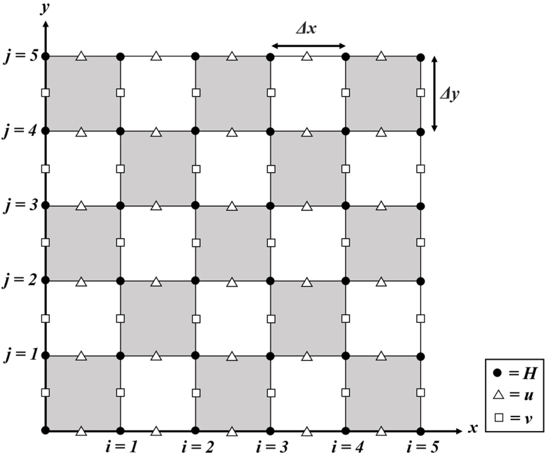
The finite difference method, named as the leapfrog method [43,44], was used to perform numerical operations from four different spatially interleaved grids. The continuous differential operator in the original partial differential equation would be replaced with the spatially discretized differential operator to obtain the discrete approximation. The accuracy of the numerical analysis depends on the density of the grid. In this study, the Arakawa C-grid was applied for numerical computation [45,46], and the water depth at the grid points was solved by the two-dimensional depth-averaged velocity field (as shown in Figure 4).
Under steady flow conditions, the two-dimensional continuity equation (Equation (4)) can be organized into a finite-difference first-order leapfrog format to solve for the water level:
Equation (6) has second-order accuracy in both x and y directions and can be numerically solved for the continuity equation. The boundary conditions of this study were set as follows to solve water depths at each grid points: upstream boundary water depth equals to initial water depth, and the sidewall water depth was defined as . The Courant–Friedrichs–Lewy (CFL) is necessary for convergence to have an interdependent relationship between the domain of parametric values derived from initial conditions and the approximation method for all grid points. By limiting the maximum step size of the grid spacing, the stability of the numerical analysis is ensured. The CFL condition for this study is:
3. Experimental Setup
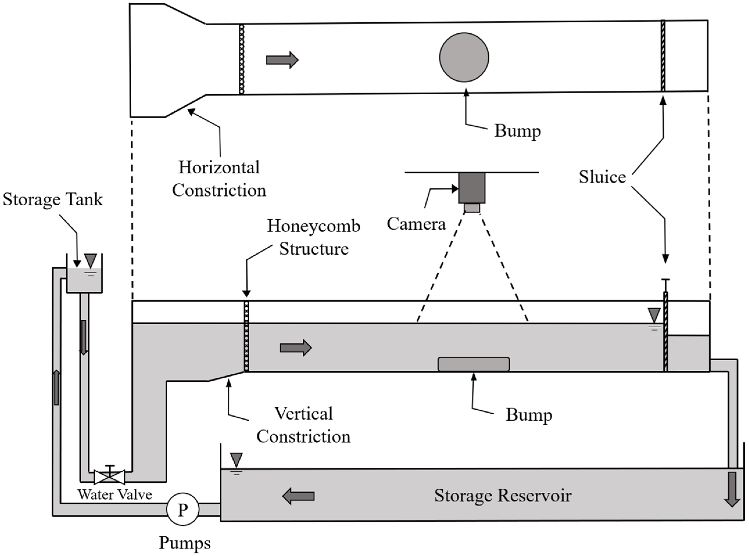
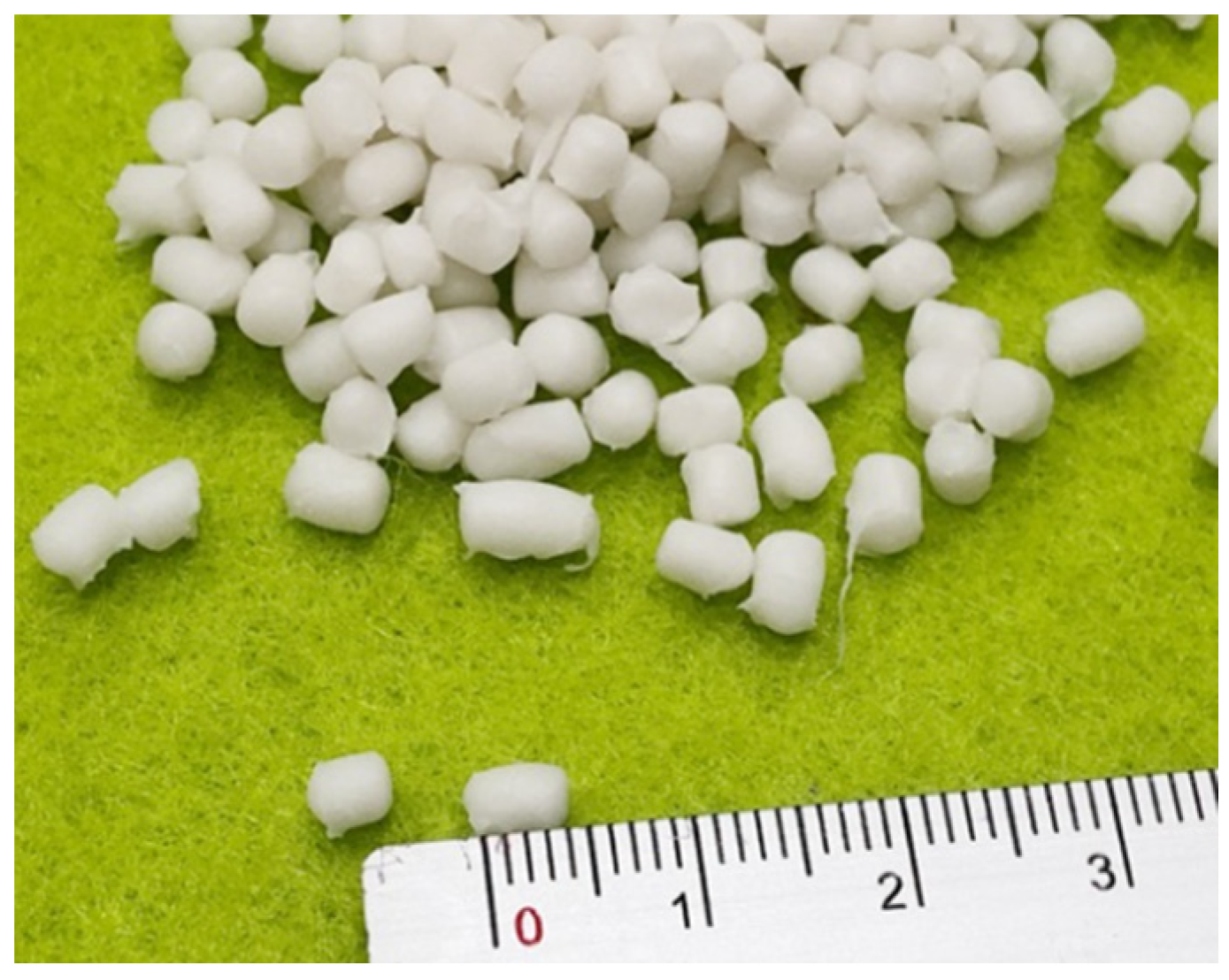
The study was conducted in a 30 m long, 1 m wide, 1 m high circulating flume in the Hydrotech Research Institute at National Taiwan University, Taiwan. The flow rate and water depth were controlled by the valve and the tailgate, respectively. To ensure that the flow in the experimental section is uniform with a smooth water surface, the horizontal and vertical condensation structures were placed upstream of the flume to reduce turbulence. Furthermore, the experimental section was located 18 m downstream of the condensation section, and the camera (GoPro Hero 8) (GoPro, Inc., SanMateo, CA, USA) with linear mode, 1920 × 1080 pixels and 60 frames per second (FPS), was fixed 1.5 m above the bottom bed structures (Figure 5). The field of view (FOV) was set to be 2.2 m × 1.2 m. The control points were located on both sides for orthorectification, and the tracers of the experiment were all-white rubber particles of thermoplastic elastomer (TPE) with a size of 4 mm (as shown in Figure 6). The particle size is large enough to provide the camera to capture its pixel position efficiently and can float entirely on the water surface with good fluid tracking performance.
To test the feasibility of using the continuity equation estimating underwater topography in different flow conditions, this study set up a saucer plate, pie plate, triangle plate, square plate, and bump base plates, respectively, in the experimental section (as shown in Figure 7). Each base model was made of laminated wood, and the outer layer was painted with black paint to increase the contrast of the image.
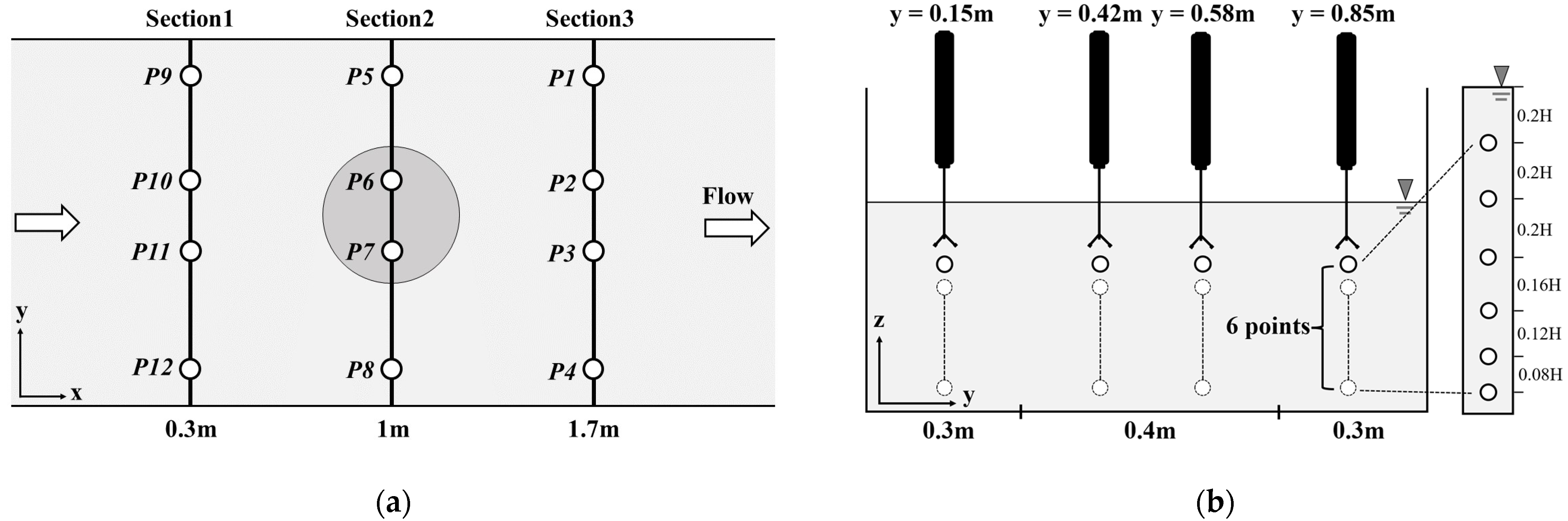
In this study, the water level was varied by adjusting the tailgate under a fixed flow rate (Q = 0.09 m3/s), and three respective water levels of 15.5 cm, 20 cm, and 25 cm were simulated. Additionally, the upstream Froude numbers are 0.5, 0.33, and 0.22, respectively. At the same time, the data measured by the Acoustic Doppler Velocimetry (ADV) were compared with the results of the LSPIV. The SonTek 16-MHz Micro ADV (SonTek, Inc., San Diego, CA, USA) was conducted in this experiment. The sampling frequency was set to 25 Hz, and the thresholds for signal-to-noise ratio (SNR) and correlation, were 15 dB and 70%, respectively. The sampling point was located at 5 cm below the probe, and the sampling volume was 0.25 c.c. Furthermore, the temperature and salinity correction were performed using the Smart sensor AR8012 handheld salinometer (Shenzhen Mreay Electronic Commerce Co., Ltd., Shenzhen, China). Additionally, the ADV was used to measure 12 locations in three cross-sections of the model: upstream, midstream, and downstream (Figure 8), and at each location, there were 6 measurement points from bottom to near-surface. To avoid errors caused by transient surges, the data at each measurement point were measured for at least 180 s. The results fit the vertical velocity profiles to obtain the surface velocity as a standard value for comparison. Without considering the wake effect, the fitting of the velocity profile can be defined by Equation (8) [47]:
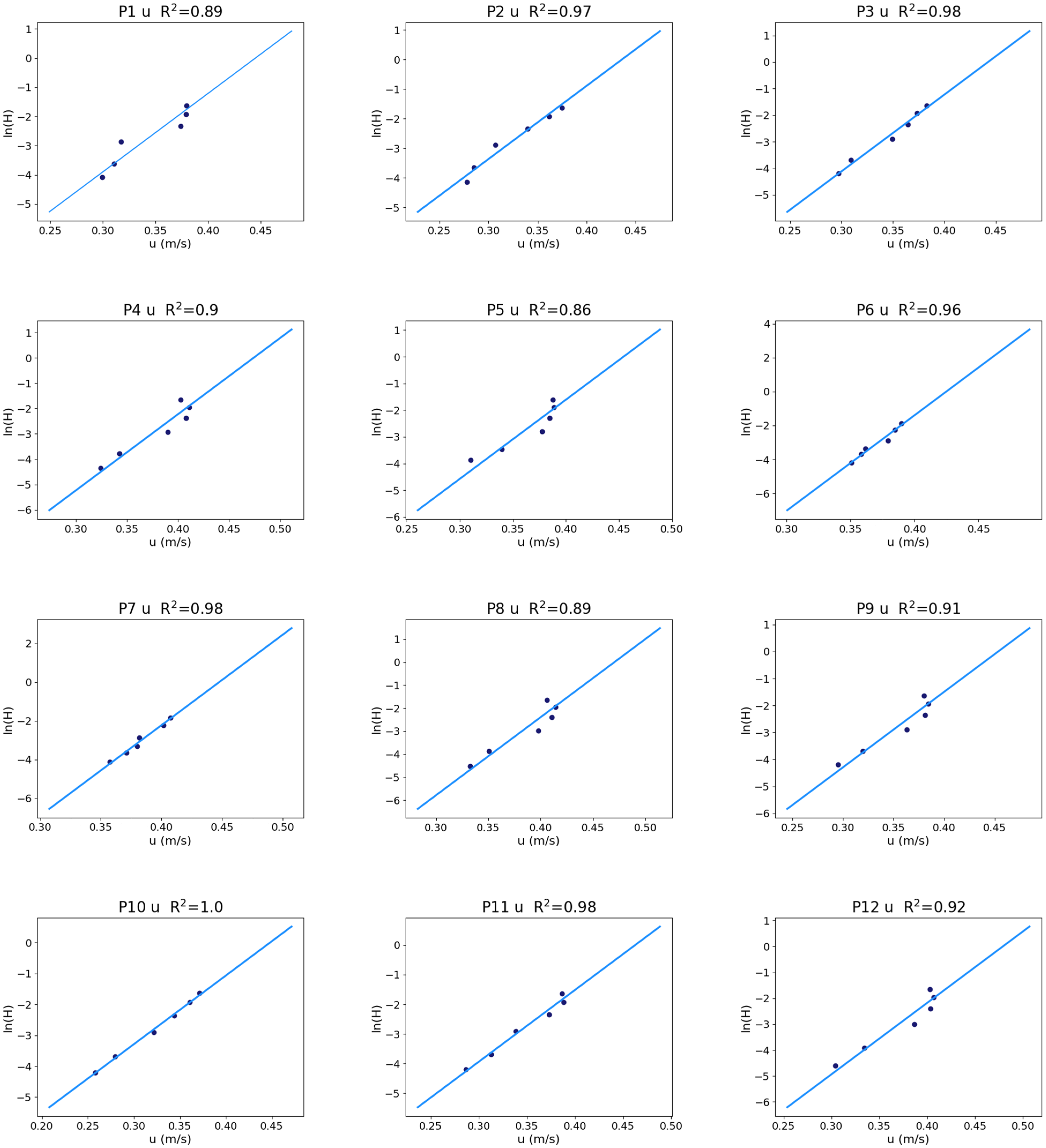
Under smooth wall conditions (, ) [48]. Equation (8) can be simplified to a linear function in logarithmic form:
By substituting the measured flow velocity values at 6 different depths into Equation (9), the velocity profile can be fitted and the surface velocity at the measurement point can obtained by extrapolating.
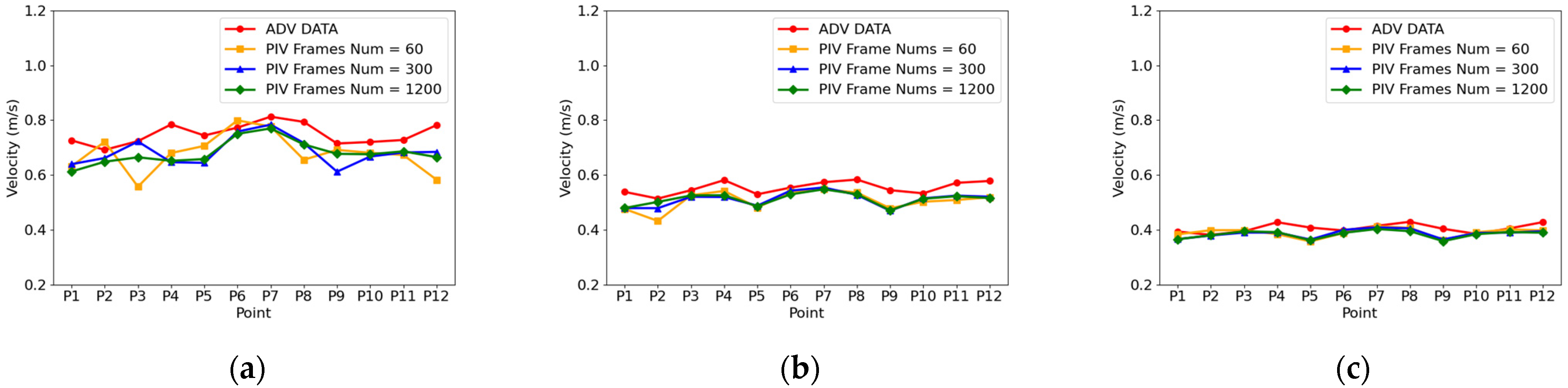
For the LSPIV, three types of IAs, 32 × 32, 64 × 64, and 128 × 128, were used for calculations, and 60 (1 s), 300 (5 s), and 1200 (20 s) successive images were selected at 60 fps. The results of all surface velocity analysis were compared with the ADV data, and the best surface velocity data was selected for subsequent water depth calculation by the average relative error assessment.
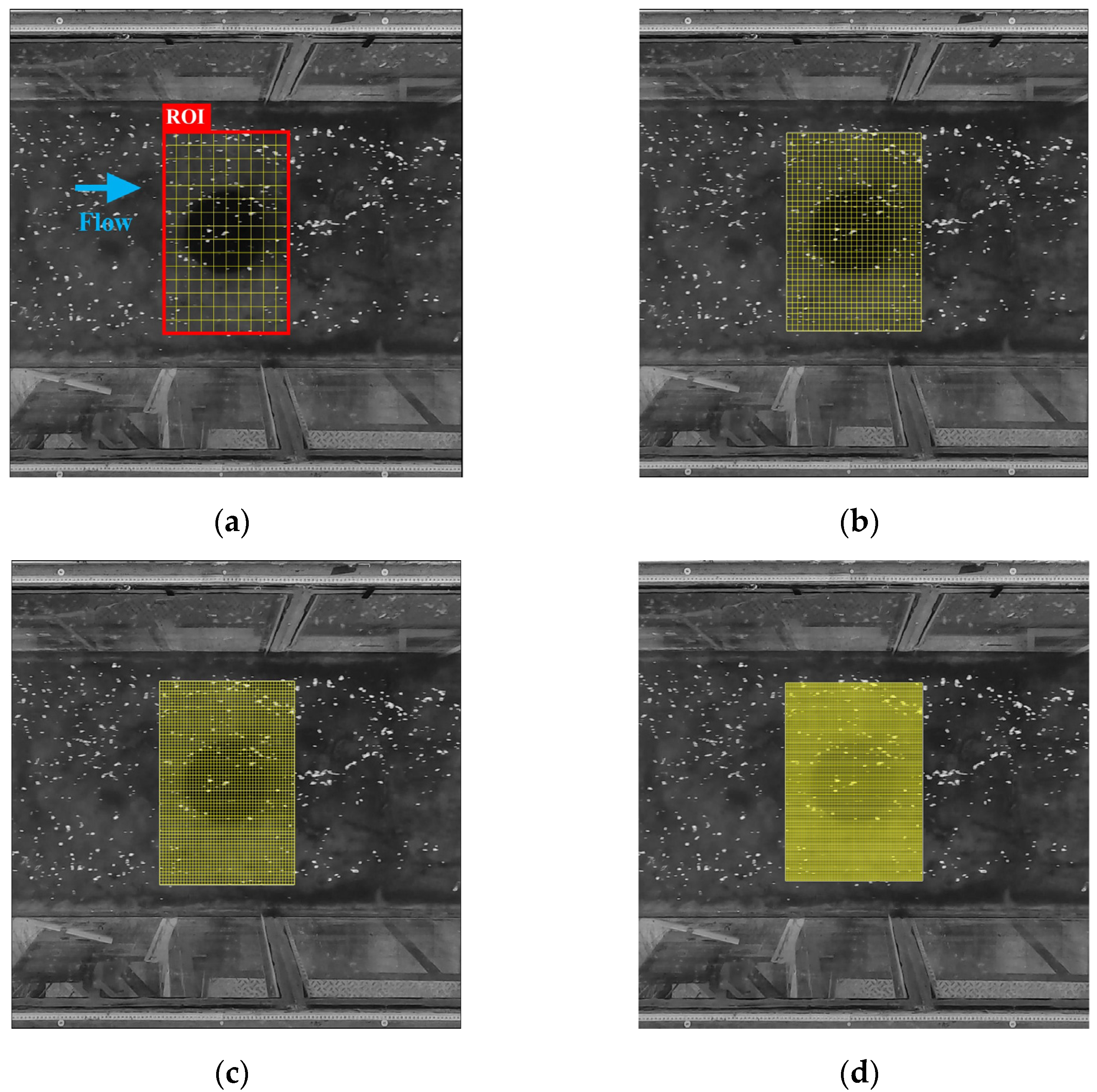
After obtaining the depth-averaged velocities by scaling the surface ones with a factor k = 0.85, Equation (6) can be used to calculate the water depth. At the center of the model, a rectangular area of 55 cm in length and 75 cm in width in the vertical direction was first selected as the region of interest (ROI) for numerical analysis. The effect of water depth and mesh density on the bathymetry calculation then was compared under three flow conditions of 15.5 cm, 20 cm, and 25 cm water depths, with 10 × 15 (about 5 cm2), 25 × 35 (about 2 cm2), 45 × 65 (about 1.08 cm2), and 90 × 125 (about 0.5 cm2) meshes under CFL conditions (as shown in Figure 9). The comparison between the physical model and the estimated bathymetry of the root-mean-square error (RMSE) of the vertical and horizontal elevation profiles was used to evaluate the reliability of the proposed method.
4. Results and Discussion
4.1. ADV Results
The ADV measured 12 locations in the upper, middle, and lower reaches of the model, fitted the vertical flow profiles, and estimated the surface flow velocity. The results showed that the values of the 12 fitted profiles were all above = 0.85 and in accordance with the log-law distribution, the SNR values of the samples were all maintained at 30 dB or less, and the correlation was stable at about 80% (as shown in Figure 10). Therefore, the surface velocities of the 12 locations estimated from the ADV velocity profiles can be used as benchmark values for comparison with the LSPIV results.
4.2. Comparison with Different Interrogation Areas
Three sets of subimage sizes commonly found in PIV, namely 32 × 32, 64 × 64, and 128 × 128, were used to compute the three water depths over the saucer plate. The searching area (SA) was set to 15 pixels in the downstream direction and 5 pixels in the rest of the directions, and such a parameter configuration could ensure the smooth matching of two successive images and compute the correlation matrix with less uncertainty. The test results are evaluated by comparing the average relative error, which is calculated as follows:
The comparison results of different IA sizes show that the average relative error of surface velocity is larger than 15% for the IA of 32 × 32 pixels, which is higher than the error values of other subimage sizes, regardless of the water depth conditions (see Figure 11). The IA size of 64 × 64 pixels is better than 128 × 128 pixels, so it is clear that the IA size of 64 × 64 pixels is the most suitable for the experimental configuration of this study. A small IA size will not provide good results for tracking particle features in subimages; however, a large IA size might include too many features, which will reduce the resolution of velocity field and produce more bias. In general, the surface flow velocity values measured by the images are very close to the ADV measurements, and the accuracy can reach 92.7% (see Table 1).
4.3. Comparison with Different Frame Rates
The frame rate of the image is also an important parameter of the LSPIV. Generally speaking, to obtain good results, it is recommended to run a larger frame rate for calculation. However, the increasing images will increase the calculation time and reduce the ability to measure the instantaneous velocity. Selecting the appropriate number of frames for the image analysis would lead good results within a reasonable calculation time. Figure 12 shows the calculation results of 60 frames (1 s), 300 frames (5 s), and 1200 frames (20 s), with three different of water depths. When the water depth is 15.5 cm, the average relative error generated by using 60 frames is greater than 10%, while the error of 300 frames and 1200 frames is less than 10%. The main reason is that, in a smaller frame, the flow velocity is faster, and the particles of the subimage enter and exit the SA range in a shorter time. The error, then, is caused by the fewer samples. However, when the water depth increases to 20 and 25 cm, the error can be reduced to 7.58% and 4.82%, respectively (see Table 2). Overall, the calculated two-dimensional surface velocity can represent the velocity field as long as using more than 300 frames.
4.4. LSPIV Surface Velocity
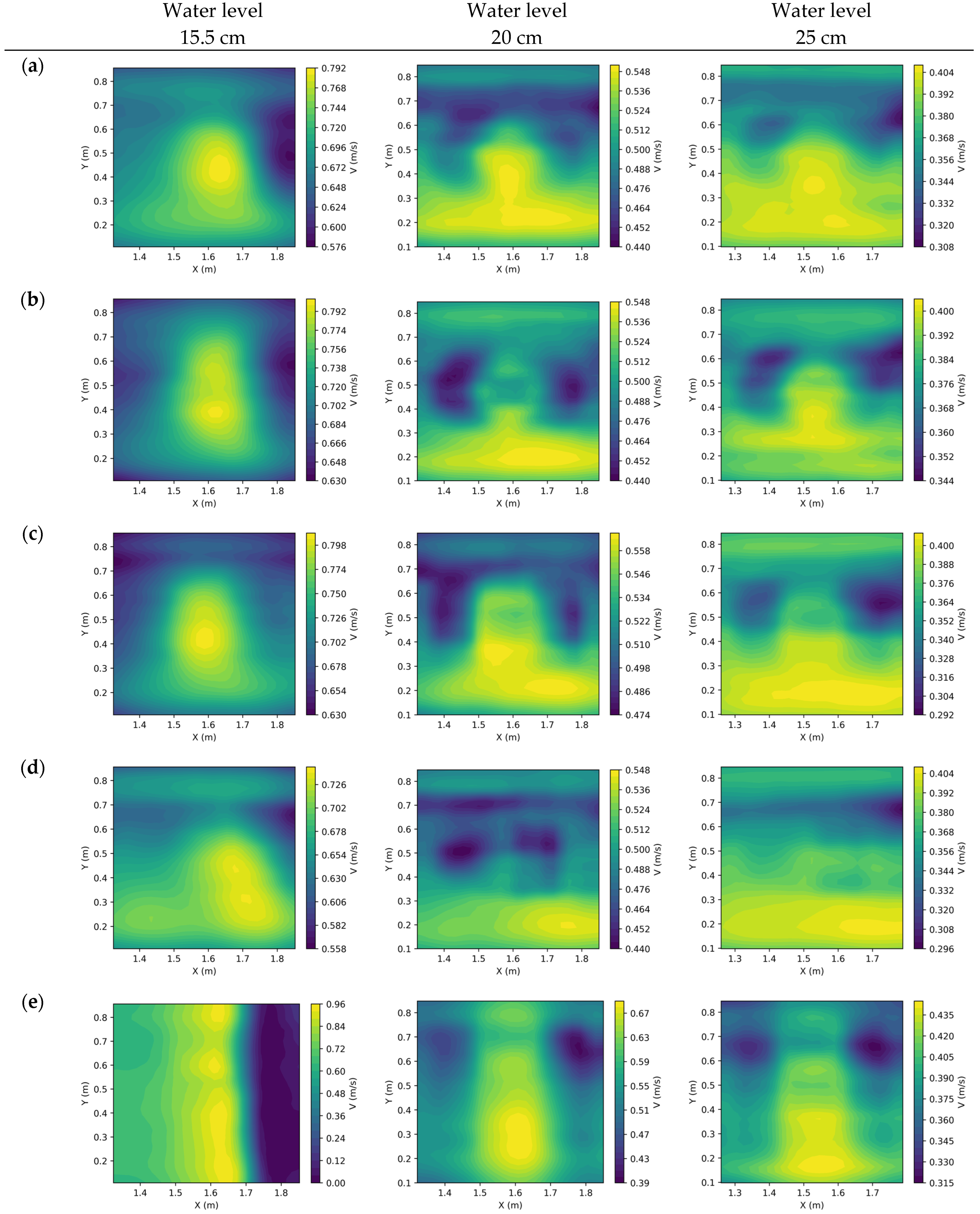
Figure 13 shows the two-dimensional surface velocity fields calculated using particle images with differently shaped bed models at different water depths. Additionally, the length represents the flow direction and the width represents the cross direction of the flume. The movement of the flow is from left to right, and the center coordinates of each model are located at (1.588 m, 0.482 m). When the water depth is 15.5 cm, the flow field in the downhill section behind the bump model changes from a subcritical flow to a supercritical flow due to the shallow water, resulting in a hydraulic jump, which causes the particles to be swept in and lose trackability, and which clearly distorts the 2D surface velocity calculation. When the water depth is 20 cm, the difference between the high and low velocities of the velocity field becomes more obscure, especially for the surface velocity profile of the triangular bottom bed. It was initially concluded that the surface velocity did not accelerate as much as expected because the model itself was the smallest among all. In addition, the model was installed with the triangular tip toward the upstream direction, which makes the overall shape more streamlined. The flow through the model is thus less disturbed and cannot adversely affect the surface flow field. When the water depth reaches 25 cm, the bottom bed model has less influence on the surface velocity.
4.5. Comparison of Different Mesh Settings
The continuity equation is solved with the frog-jumping method and the two-dimensional surface velocity. The two-dimensional water depth distribution for different test occasions can then be determined. The mesh density is a crucial influence factor in the solution process. The research results show that when the water depth is 15.5 cm and the grid is set to 10 × 15 (5 cm), the resolution is low because the spacing is too large, the discontinuity between the grids is too significant, and the contour line has many angles, leading to errors. When the grid size is set to 45 × 65 (1.08 cm), the contour lines start to show horizontal stripes, and when the grid size is reduced to 90 × 125 (0.5 cm), the horizontal stripes become more prominent (Figure 14). The occasion shows that the overlap rate of the subimages of particle image velocimetry is too high for the dense grids. When the density of the traced particles is not sufficient, the same particle characteristics will be repeatedly calculated, causing the two-dimensional flow field to produce stripes in the velocity direction and resulting in measurement bias. In this study, the most suitable grid size is 25 × 35 (2 cm), which will be used for numerical analysis in the subsequent experiments.
4.6. Bathymetry Measurements
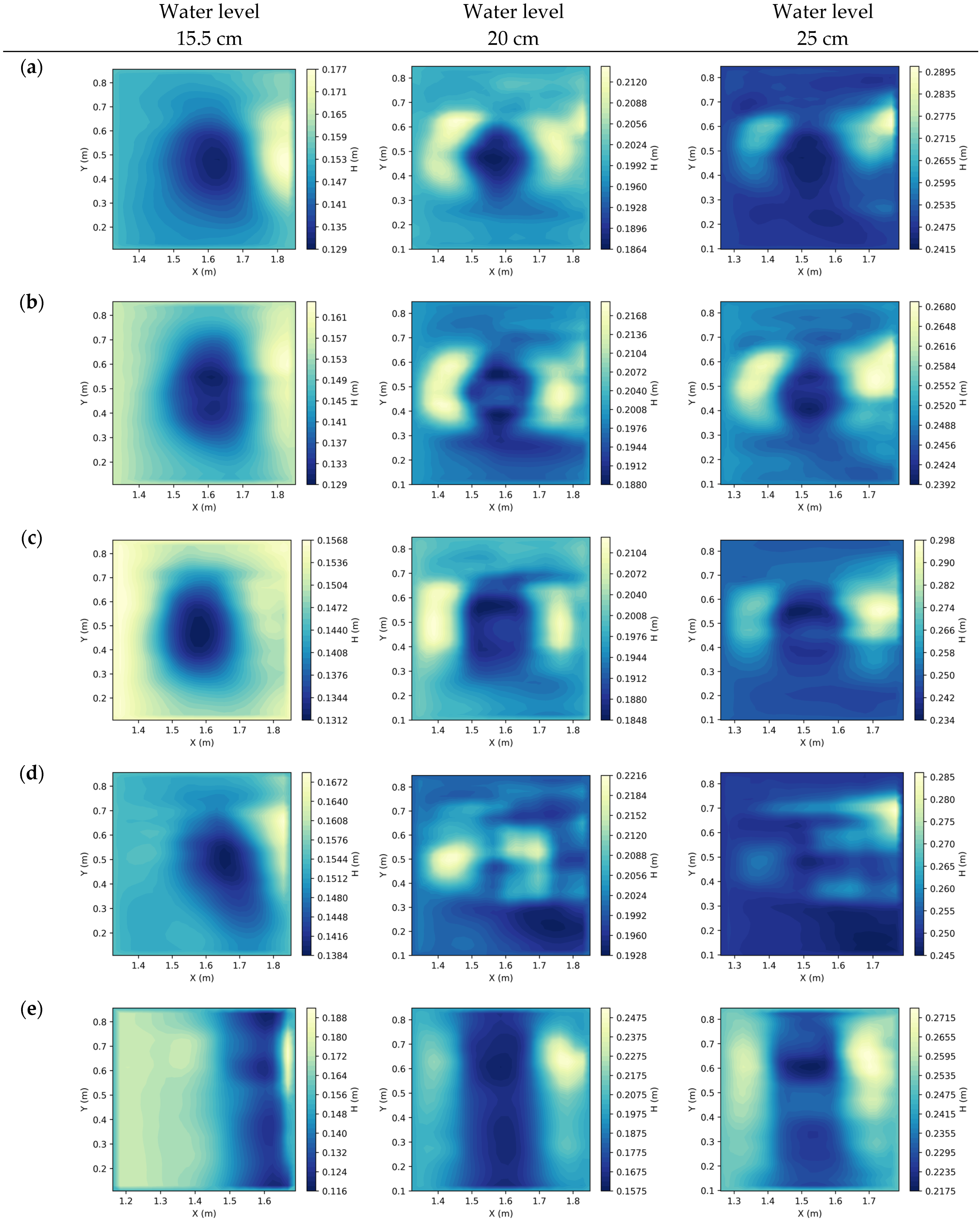
Figure 15 shows the results of the measured water depth of different bed models under different water levels. The results showed that, when the water level is 15.5 cm, the water depth measurements near the model decreased, which is consistent to the actual observation. Meanwhile, the gradient distribution of water depth shows that the water is shallower near the model’s center. This is correlated to the inverse relationship between surface flow rate and water depth at a fixed flow rate. The results also demonstrate the nonintrusive method can successfully capture the water depth variation caused by the bed elevation. For the saucer plate and bump, the LSPIV method combined with the continuity equation was able to capture the shape contour under different water levels. For pie, square, and triangular plates, when the water level increased to 25 cm, the relative magnitude of the change in water depth decreased and the measurements before and after the model were deeper than actual values. An upward force occurs in front of the model when the flow passes through the bedform model. At the same time, vorticity is caused by the decrease in bed elevation behind the model. The rapid decrease in the surface flow velocity caused by the vorticity is then detected as an error.
To quantitatively evaluate the capability of the proposed method in capturing the bed elevation, the measurements were compared with the longitudinal and lateral profile of the models divided based on the center point. Furthermore, the RMSE evaluated the elevation error in the longitudinal and lateral profiles at each grid point. Finally, the impact of the water level on the bed elevation measurements is evaluated by dividing the measured water depths by the water level. The expression of RMSE is:
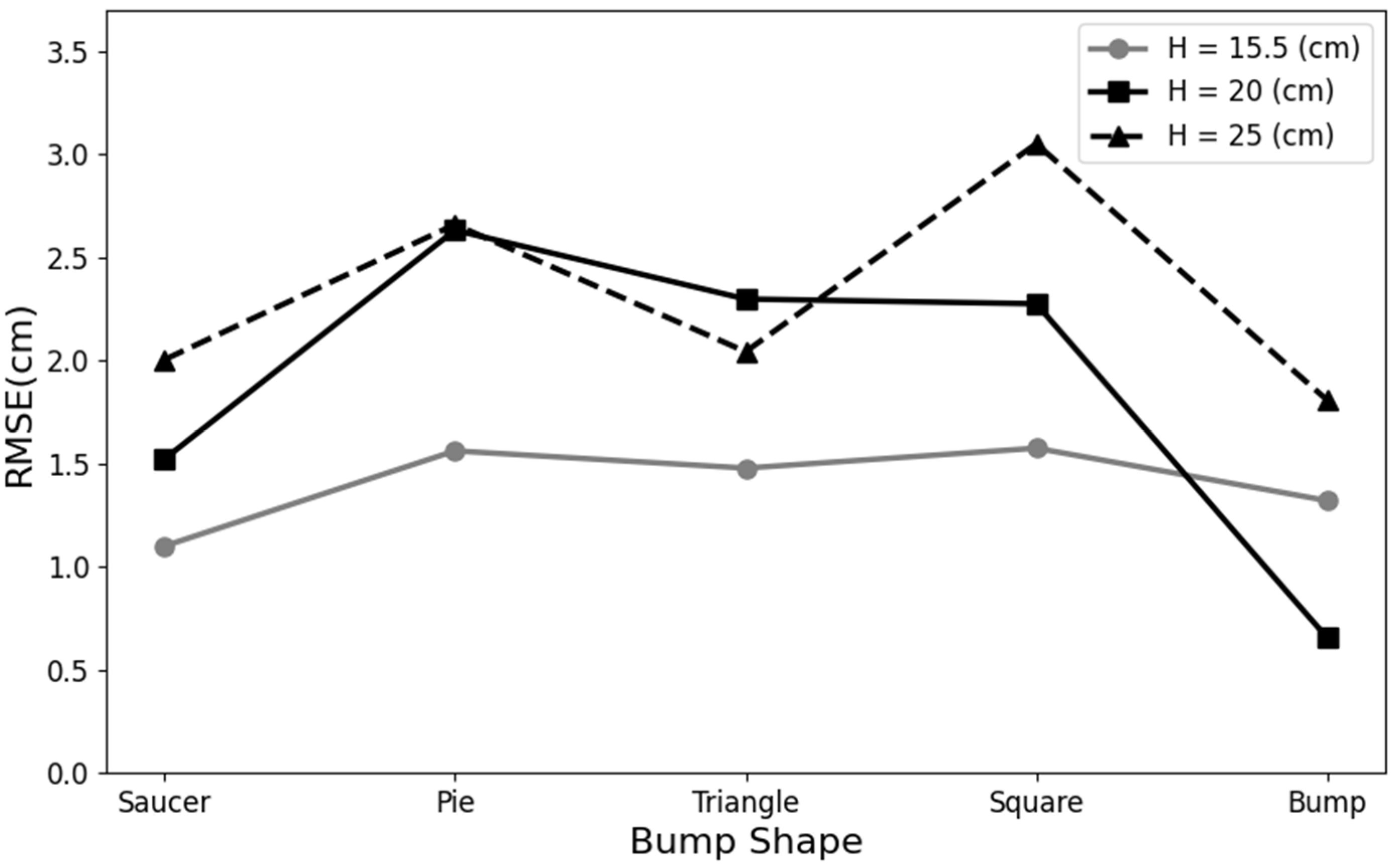
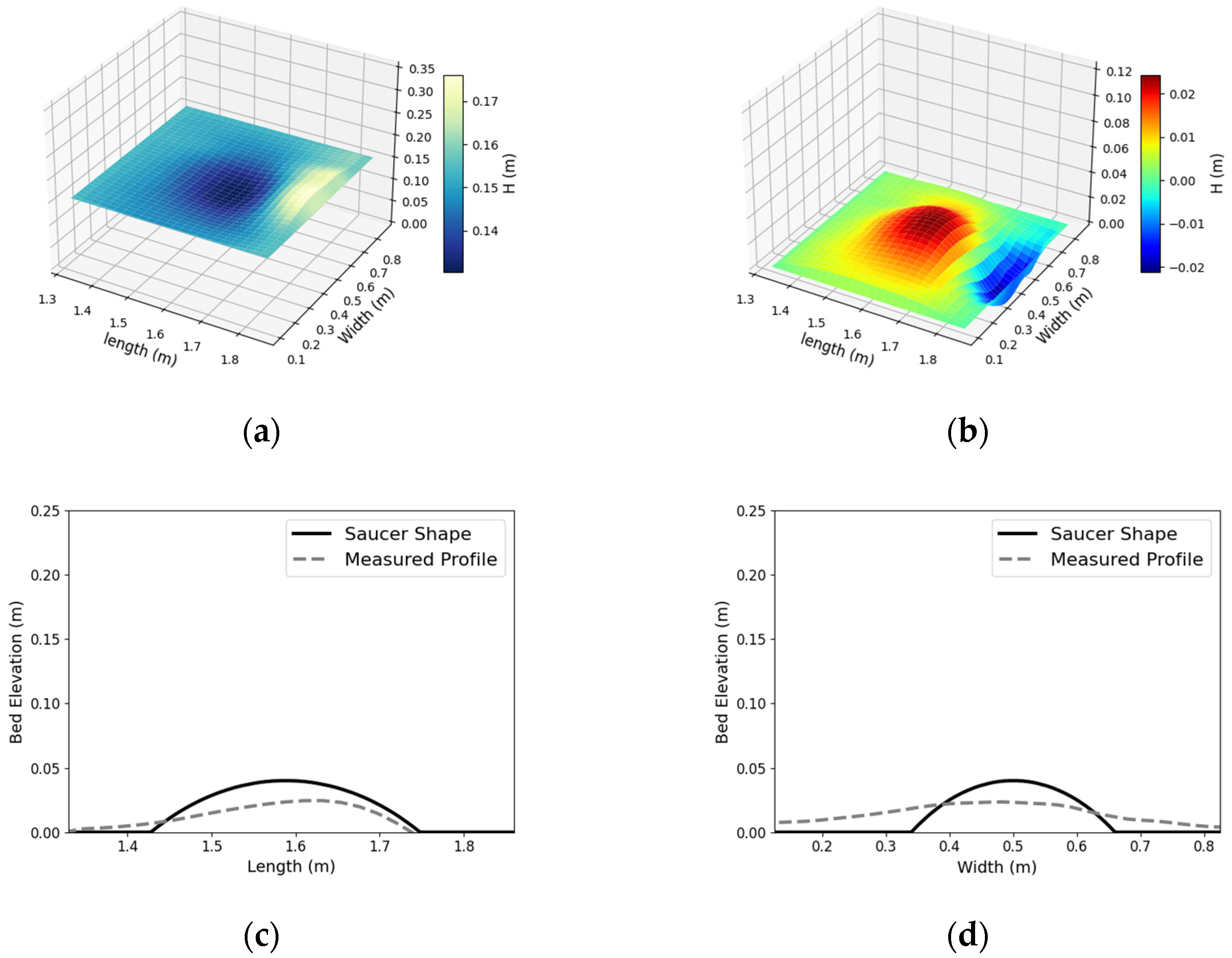
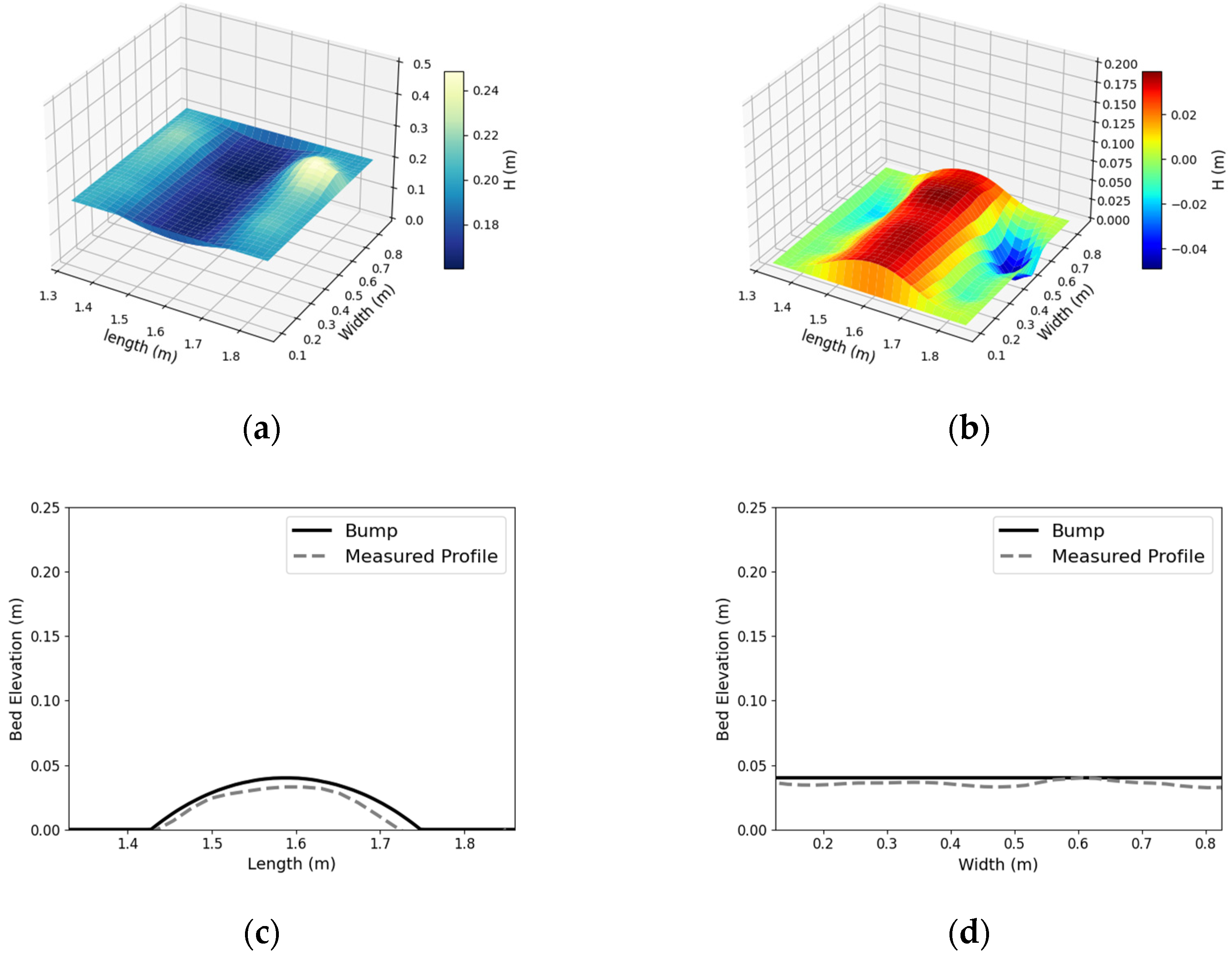
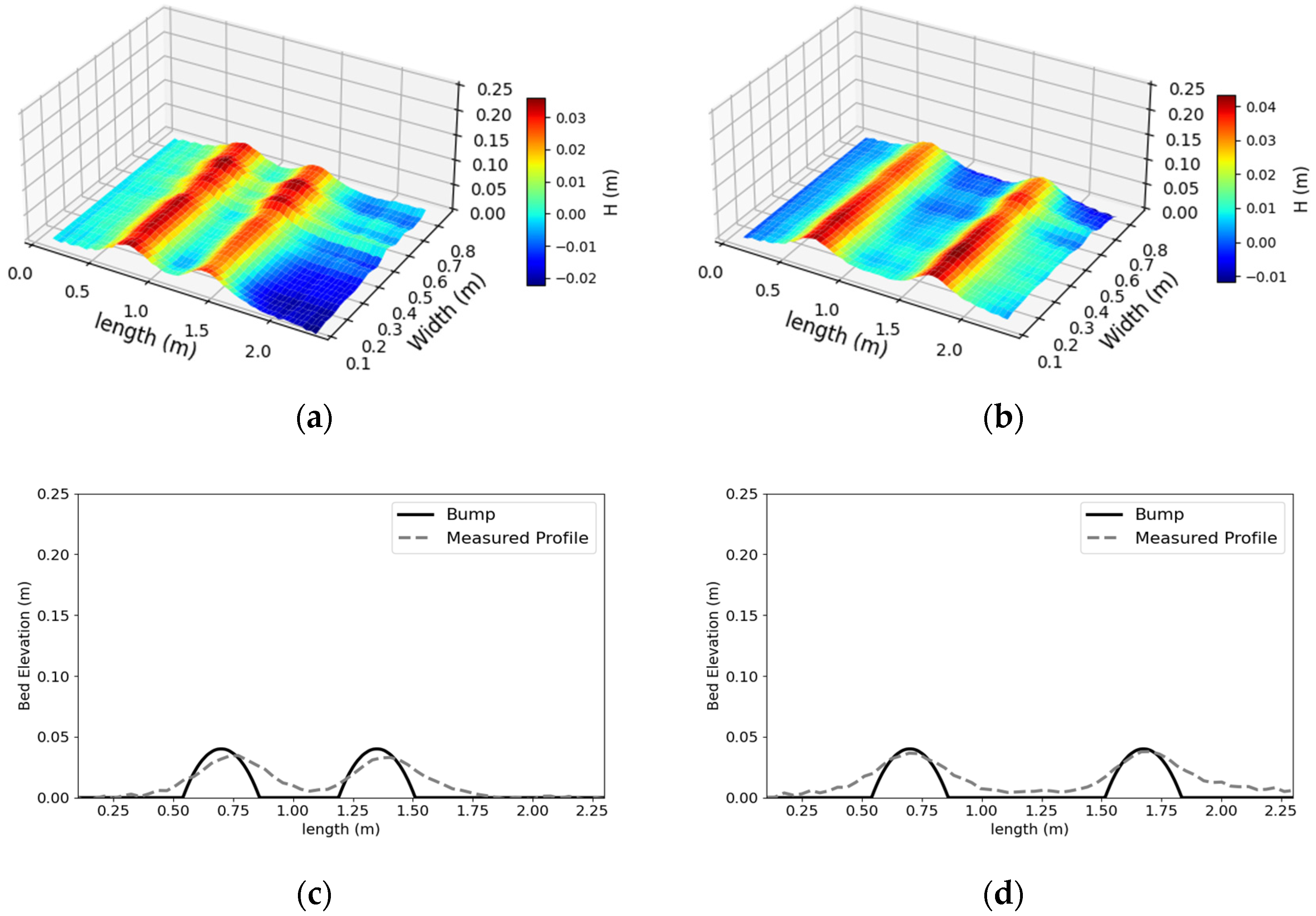
Figure 16 shows the comparison of the error of the bed elevation measurements. The results show that, when the water level was shallow, applying the proposed method could obtain relatively good results. However, when the water level gradually increased, the physical properties of the continuity equation were reduced and might cause errors. It is inferred that the three models’ (pie, square, and triangular plates) abrupt changes in their edges would affect the surface velocity and interfere with the elevation calculation results. Additionally, the velocity profile above the model is affected by intersecting with the lateral flow caused by the shape of the bedform. The incident will decrease the overall surface velocity and underestimate the bed elevation. As for the saucer plate and bump, the edges changed progressively without obvious ridges, and the bump was across the section, which distributes less influence by lateral flow; therefore, the bed elevation and water depth measurements were close to the actual observation (Figure 17a,b and Figure 18a,b). The comparison of bed profiles demonstrated that the proposed method can accurately delineate the bedform (see Figure 17c,d and Figure 18c,d).
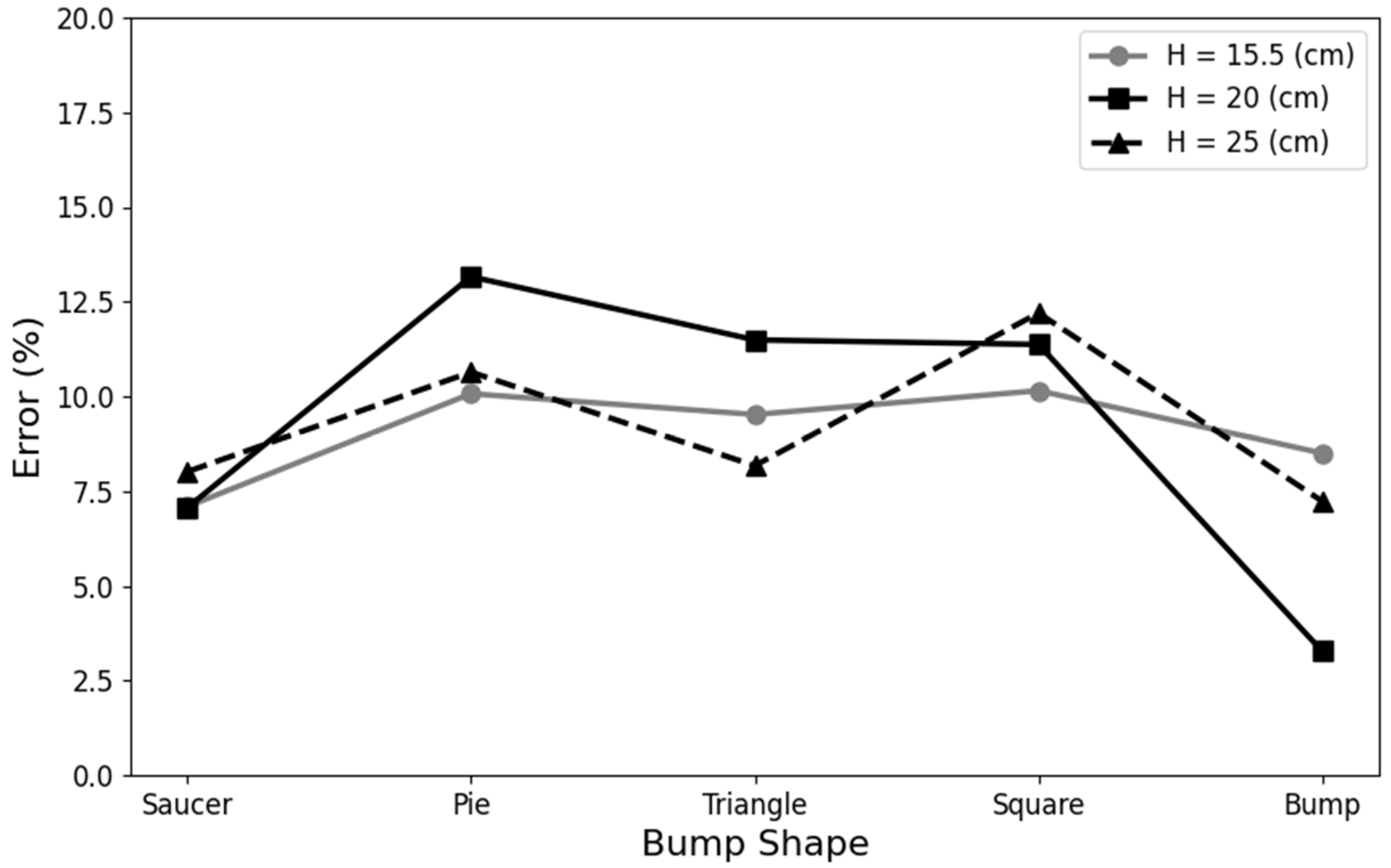
To evaluate the overall error of the bed elevation and the effect of water levels, the RMSE was divided by the water level for each test. The results showed that the average error is around 9% regardless of the water levels (Figure 19). Although the RMSE value increases with the water level, the error can be controlled within a reasonable range. Therefore, the use of the LSPIV combined with solving the continuity equation for the bedform measurement can indeed show the changes of the bed elevation, and the average accuracy can reach 90.8% in this study.
4.7. Comparison with Composite Bed Structures
Two distinct sets of continuous bump base plates were designed for numerical analysis to evaluate the feasibility of the composite bed structures. The spacing of these two groups of bumps is one time and two times the width of the bumps. As a result (Figure 20), this method can accurately delineate the bedform regardless of the continuous bump spacing combination. Furthermore, the average RMSE can be controlled below 0.9 cm. It shows that the method in this study has the potential to invert the complex bedform, and possibilities for field measurement.
5. Conclusions and Discussion
This study demonstrates that a nonintrusive method for solving the continuity equation for shallow water equations using the LSPIV and the leapfrog method has the potential to measure a large range of 2D bed elevations in open channel flow. Although the difference of IA sizes and frame rates may cause the calculation error, the results show that the surface velocity field can be calculated with more than 90% accuracy by using more than 300 frames at 60 fps.
In this study, four different grid density sizes were used for numerical analysis. The comparison results showed that the loose grids would cause discontinuity, while the dense grids would increase the overlap rate and affect the analysis results. The results express that the proper grid size is 2 cm. Meanwhile, it shows that the capability to measure bed elevation is inversely proportional to the water depth, and the average RMSE of the bed elevation measurements is below 1.6 cm when the water depth is shallow. The overall average accuracy was 90.8% with respect to the total water depth. The experimental results demonstrate that the velocity measurements combined with continuity equation can be the means to estimate the bed variation trend and enhance the potential application of image techniques for flow measurements. Although the proposed method should be limited to the straight channel, shallow water depth, and the simple bed forms, the image measurements combined with the hydraulic modeling show the potential to provide the approximate bathymetry in the field. Compared with traditional flow measurement, this approach has the advantages of automatic measurements and the integration with Internet of Things (IoT) to provide real-time remote monitoring data. In addition, its low construction cost (about 1% of the traditional methods) can effectively improve the coverage of measurement stations and construct a complete hydrometric monitoring network to enhance the efficiency of the water resource management. In recent years, the equipment has developed rapidly, both cameras and uncrewed aerial vehicles have gradually become more popular, and their performance has been increasingly improved, and it has become easier to obtain high pixel and high frame-rate images. The use of this image technique as a main measurement tool is increasingly feasible and can reduce the risk and cost of in situ measurements.
Author Contributions
Conceptualization, H.-C.H.; methodology, H.-C.H. and Y.-C.L.; formal analysis, Y.-C.L. and H.-Y.C.; investigation, Y.-C.L.; data curation, H.-C.H. and H.-Y.C.; writing—original draft preparation, H.-C.H. and Y.-C.L.; writing—review and editing, T.-A.L.; Visualization, Y.-C.L.; funding acquisition, H.-C.H. All authors have read and agreed to the published version of the manuscript.
Funding
This research was funded by Ministry of Science and Technology (110-2625-M-002-024).
Institutional Review Board Statement
Not applicable.
Informed Consent Statement
Not applicable.
Data Availability Statement
Not applicable.
Conflicts of Interest
The authors declare no conflict of interest.
Abbreviation
| Symbol | Description |
| moving distance about distinct pattern | |
| time difference between each frame | |
| , | image coordinates |
| , | width and height for subimages |
| , | pixel intensity at location (, ) for subimage A and B |
| , | average pixel intensity |
| standard divination of the Gaussian kernel | |
| size of Gaussian kernel | |
| total water depth () | |
| height deviation of its mean height | |
| mean height of the horizontal pressure surface | |
| , | depth-averaged velocity in the length and width direction |
| upstream boundary water depth | |
| initial water depth | |
| sidewall water depth | |
| length of the grid | |
| width of the grid | |
| average relative error | |
| measured locations | |
| surface velocity from LSPIV | |
| surface velocity from ADV | |
| elevation of model | |
| elevation estimated with proposed method | |
| total number of grids | |
| position of z-direction | |
| x-directional velocity value of z-position | |
| shear velocity | |
| shear stress | |
| von Kármán constant | |
| constant |
References
- Loucks, D.P.; Beek, E.V. Water resources planning and management: An overview. In Water Resource Systems Planning and Management; Springer: Cham, Switzerland, 2017; pp. 1–49. [Google Scholar]
- Wu, S.-J.; Lien, H.-C.; Chang, C.-H. Modeling risk analysis for forecasting peak discharge during flooding prevention and warning operation. Stoch. Environ. Res. Risk Assess. 2010, 24, 1175–1191. [Google Scholar] [CrossRef]
- Rantz, S.E. Measurement and Computation of Streamflow; US Department of the Interior, Geological Survey: Reston, VA, USA, 1982; Volume 2175.
- Lee, C.-J.; Kim, W.; Kim, C.-Y.; Kim, D.-G. Velocity and discharge measurement using ADCP. J. Korea Water Resour. Assoc. 2005, 38, 811–824. [Google Scholar] [CrossRef] [Green Version]
- Sassi, M.; Hoitink, A.; Vermeulen, B. Discharge estimation from H-ADCP measurements in a tidal river subject to sidewall effects and a mobile bed. Water Resour. Res. 2011, 47, 1–14. [Google Scholar] [CrossRef] [Green Version]
- Kuczera, G. Correlated rating curve error in flood frequency inference. Water Resour. Res. 1996, 32, 2119–2127. [Google Scholar] [CrossRef]
- Sivapragasam, C.; Muttil, N. Discharge rating curve extension—A new approach. Water Resour. Manag. 2005, 19, 505–520. [Google Scholar] [CrossRef]
- Clarke, R.T.; Mendiondo, E.; Brusa, L. Uncertainties in mean discharges from two large South American rivers due to rating curve variability. Hydrol. Sci. J. 2000, 45, 221–236. [Google Scholar] [CrossRef]
- Westerberg, I.; Guerrero, J.L.; Seibert, J.; Beven, K.; Halldin, S. Stage-discharge uncertainty derived with a non-stationary rating curve in the Choluteca River, Honduras. Hydrol. Processes 2011, 25, 603–613. [Google Scholar] [CrossRef]
- Fujita, I.; Komura, S. Application of video image analysis for measurements of river-surface flows. Proc. Hydraul. Eng. 1994, 38, 733–738. [Google Scholar] [CrossRef]
- Bradley, A.A.; Kruger, A.; Meselhe, E.A.; Muste, M.V. Flow measurement in streams using video imagery. Water Resour. Res. 2002, 38, 51-1–51-8. [Google Scholar] [CrossRef]
- Takehara, K.; Fujita, I.; Takano, Y.; Etoh, G.T.; Aya, S.; Tamai, M.; Miyamoto, H.; Sakai, N. An atempt of field measurements of surface flow on a river by using a helicopter aided image velocimetry. Proc. Hydraul. Eng. 2002, 46, 809–814. [Google Scholar] [CrossRef] [Green Version]
- Meselhe, E.; Peeva, T.; Muste, M. Large scale particle image velocimetry for low velocity and shallow water flows. J. Hydraul. Eng. 2004, 130, 937–940. [Google Scholar] [CrossRef]
- Dermisis, D.; Papanicolaou, A. Determining the 2-D surface velocity field around hydraulic structures with the use of a large scale particle image velocimetry (LSPIV) technique. In Impacts of Global Climate Change; ASCE Library: Reston, VA, USA, 2005; pp. 1–12. [Google Scholar]
- Kim, Y. Uncertainty Analysis for Non-Intrusive Measurement of River Discharge Using Image Velocimetry; The University of Iowa: Iowa City, IA, USA, 2006. [Google Scholar]
- Lewis, Q.W.; Lindroth, E.M.; Rhoads, B.L. Integrating unmanned aerial systems and LSPIV for rapid, cost-effective stream gauging. J. Hydrol. 2018, 560, 230–246. [Google Scholar] [CrossRef]
- Tauro, F.; Pagano, C.; Phamduy, P.; Grimaldi, S.; Porfiri, M. Large-scale particle image velocimetry from an unmanned aerial vehicle. IEEE/ASME Trans. Mechatron. 2015, 20, 3269–3275. [Google Scholar] [CrossRef]
- Fujita, I. Discharge measurements of snowmelt flood by space-time image velocimetry during the night using far-infrared camera. Water 2017, 9, 269. [Google Scholar] [CrossRef]
- Gerritsen, G. Flood Wave Monitoring Using LSPIV: A Methodology for Monitoring Flood Waves in an Equatorial Urban Stream with Fast Response Time; Delft University of Technology: Delft, The Netherlands, 2020; pp. 37–47. [Google Scholar]
- Le Coz, J.; Hauet, A.; Pierrefeu, G.; Dramais, G.; Camenen, B. Performance of image-based velocimetry (LSPIV) applied to flash-flood discharge measurements in Mediterranean rivers. J. Hydrol. 2010, 394, 42–52. [Google Scholar] [CrossRef] [Green Version]
- Theule, J.I.; Crema, S.; Marchi, L.; Cavalli, M.; Comiti, F. Exploiting LSPIV to assess debris-flow velocities in the field. Nat. Hazards Earth Syst. Sci. 2018, 18, 1–13. [Google Scholar] [CrossRef] [Green Version]
- Johnson, E.; Cowen, E. Remote monitoring of volumetric discharge employing bathymetry determined from surface turbulence metrics. Water Resour. Res. 2016, 52, 2178–2193. [Google Scholar] [CrossRef] [Green Version]
- García-Navarro, P.; Murillo, J.; Fernández-Pato, J.; Echeverribar, I.; Morales-Hernández, M. The shallow water equations and their application to realistic cases. Environ. Fluid Mech. 2019, 19, 1235–1252. [Google Scholar] [CrossRef] [Green Version]
- Kinnmark, I. The Shallow Water Wave Equations: Formulation, Analysis and Application; Springer: Berlin/Heidelberg, Germany, 1986; Volume 15, pp. 159–171. [Google Scholar]
- Fraccarollo, L.; Toro, E.F. Experimental and numerical assessment of the shallow water model for two-dimensional dam-break type problems. J. Hydraul. Res. 1995, 33, 843–864. [Google Scholar] [CrossRef]
- Kocaman, S.; Güzel, H.; Evangelista, S.; Ozmen-Cagatay, H.; Viccione, G. Experimental and numerical analysis of a dam-break flow through different contraction geometries of the channel. Water 2020, 12, 1124. [Google Scholar] [CrossRef] [Green Version]
- Bao, Y.; Chen, J.; Sun, X.; Han, X.; Li, Y.; Zhang, Y.; Gu, F.; Wang, J. Debris flow prediction and prevention in reservoir area based on finite volume type shallow-water model: A case study of pumped-storage hydroelectric power station site in Yi County, Hebei, China. Environ. Earth Sci. 2019, 78, 1–16. [Google Scholar] [CrossRef]
- Gao, L.; Zhang, L.M.; Chen, H.; Shen, P. Simulating debris flow mobility in urban settings. Eng. Geol. 2016, 214, 67–78. [Google Scholar] [CrossRef]
- Ferrolino, A.; Mendoza, R.; Magdalena, I.; Lope, J.E. Application of particle swarm optimization in optimal placement of tsunami sensors. PeerJ Comput. Sci. 2020, 6, e333. [Google Scholar] [CrossRef] [PubMed]
- Ha, T.; Cho, Y.-S. Tsunami propagation over varying water depths. Ocean. Eng. 2015, 101, 67–77. [Google Scholar] [CrossRef]
- Mesinger, F.; Arakawa, A. Numerical methods used in atmospheric models. Glob. Atmos. Res. Programme 1976, 1, 9–21. [Google Scholar]
- Zhou, W. An alternative leapfrog scheme for surface gravity wave equations. J. Atmos. Ocean. Technol. 2002, 19, 1415–1423. [Google Scholar] [CrossRef]
- Pudjaprasetya, S.R. Transport Phenomena, Equations and Numerical Methods; Wiley: Hoboken, NJ, USA, 2018; pp. 101–106. [Google Scholar]
- Stelling, G.S.; Duinmeijer, S.A. A staggered conservative scheme for every Froude number in rapidly varied shallow water flows. Int. J. Numer. Methods Fluids 2003, 43, 1329–1354. [Google Scholar] [CrossRef]
- Hauet, A.; Morlot, T.; Daubagnan, L. Velocity Profile and Depth-Averaged to Surface Velocity in Natural Streams: A Review over Alarge Sample of Rivers, E3s Web of Conferences; EDP Sciences: Les Ulis, France, 2018; Volume 40, p. 06015. [Google Scholar]
- Muste, M.; Fujita, I.; Hauet, A. Large-scale particle image velocimetry for measurements in riverine environments. Water Resour. Res. 2008, 44, 4–6. [Google Scholar] [CrossRef] [Green Version]
- Muste, M.; Ho, H.-C.; Kim, D. Considerations on direct stream flow measurements using video imagery: Outlook and research needs. J. Hydro-Environ. Res. 2011, 5, 289–300. [Google Scholar] [CrossRef]
- Welber, M.; Le Coz, J.; Laronne, J.B.; Zolezzi, G.; Zamler, D.; Dramais, G.; Hauet, A.; Salvaro, M. Field assessment of noncontact stream gauging using portable surface velocity radars (SVR). Water Resour. Res. 2016, 52, 1108–1126. [Google Scholar] [CrossRef] [Green Version]
- Fujita, I.; Aya, S. Refinement of LSPIV technique for monitoring river surface flows. In Building Partnerships; ASCE Library: Reston, VA, USA, 2000; pp. 1–9. [Google Scholar]
- Kantoush, S.A.; Schleiss, A.J.; Sumi, T.; Murasaki, M. LSPIV implementation for environmental flow in various laboratory and field cases. J. Hydro-Environ. Res. 2011, 5, 263–276. [Google Scholar] [CrossRef] [Green Version]
- Fujita, I.; Muste, M.; Kruger, A. Large-scale particle image velocimetry for flow analysis in hydraulic engineering applications. J. Hydraul. Res. 1998, 36, 397–414. [Google Scholar] [CrossRef]
- Delis, A.I.; Nikolos, I.K. Shallow Water Equations in Hydraulics: Modeling, Numerics and Applications; Multidisciplinary Digital Publishing Institute: Basel, Switzerland, 2021; Volume 13, p. 3598. [Google Scholar]
- Altaie, H.; Dreyfuss, P. Numerical Solutions for 2D Depth-Averaged Shallow Water Equations; International Mathematical Forum: Ruse, Bulgaria, 2018; pp. 79–90. [Google Scholar]
- Goto, C.; Ogawa, Y.; Shuto, N.; Imamura, F. IUGG/IOC time project: Numerical method of tsunami simulation with the leapfrog scheme. Intergov. Oceanogr. Comm. UNESCO Man. Guides 1997, 35, 130. [Google Scholar]
- Griffiths, S.D. Kelvin wave propagation along straight boundaries in C-grid finite-difference models. J. Comput. Phys. 2013, 255, 639–659. [Google Scholar] [CrossRef] [Green Version]
- Kleptsova, O.; Pietrzak, J.; Stelling, G. On the accurate and stable reconstruction of tangential velocities in C-grid ocean models. Ocean. Model. 2009, 28, 118–126. [Google Scholar] [CrossRef]
- Cebeci, T. Analysis of Turbulent Boundary Layers; Elsevier: Amsterdam, The Netherlands, 2012. [Google Scholar]
- White, F.M.; Majdalani, J. Viscous Fluid Flow; McGraw-Hill: New York, NY, USA, 2006; Volume 3. [Google Scholar]
Figure 1.
Flow chart of the Large-Scale Particle Image Velocimetry (LSPIV) (FOV represents the Field of View; GRPs represents the Ground Reference Points; IA represents the Interrogation Area; SA represents the Searching Area).
Figure 1.
Flow chart of the Large-Scale Particle Image Velocimetry (LSPIV) (FOV represents the Field of View; GRPs represents the Ground Reference Points; IA represents the Interrogation Area; SA represents the Searching Area).

Figure 2.
The convolution between kernel and original image.

Figure 3.
The flow-chart about image processing (* represents the velocity component after image processing).
Figure 3.
The flow-chart about image processing (* represents the velocity component after image processing).

Figure 4.
The demonstration of Arakawa C-grid for numerical calculation.

Figure 5.
Experimental setup for the flume.

Figure 6.
TPE tracers.

Figure 7.
Bedform models used in flume: (a) saucer plate; (b) pie plate; (c) square plate; (d) triangle plate; (e) bump.
Figure 7.
Bedform models used in flume: (a) saucer plate; (b) pie plate; (c) square plate; (d) triangle plate; (e) bump.

Figure 8.
Measurement points, locations, and sections from ADV: (a) top view of the flume; (b) lateral view of the flume.
Figure 8.
Measurement points, locations, and sections from ADV: (a) top view of the flume; (b) lateral view of the flume.

Figure 9.
The mesh configuration for numerical analysis: (a) 10 × 15; (b) 25 × 35; (c) 45 × 65; (d) 90 × 125.
Figure 9.
The mesh configuration for numerical analysis: (a) 10 × 15; (b) 25 × 35; (c) 45 × 65; (d) 90 × 125.

Figure 10.
Velocity measurements along vertical profile from ADV (flume water level = 25 cm).

Figure 11.
Surface velocities measured with IAs: (a) flume water level = 15.5 cm; (b) flume water level = 20 cm; (c) flume water level = 25 cm.
Figure 11.
Surface velocities measured with IAs: (a) flume water level = 15.5 cm; (b) flume water level = 20 cm; (c) flume water level = 25 cm.

Figure 12.
Surface velocities measured with different frames: (a) flume water level = 15.5 cm; (b) flume water level = 20 cm; (c) flume water level = 25 cm.
Figure 12.
Surface velocities measured with different frames: (a) flume water level = 15.5 cm; (b) flume water level = 20 cm; (c) flume water level = 25 cm.

Figure 13.
Velocity contour obtained by LSPIV: (a) saucer plate; (b) pie plate; (c) square plate; (d) triangle plate; (e) bump.
Figure 13.
Velocity contour obtained by LSPIV: (a) saucer plate; (b) pie plate; (c) square plate; (d) triangle plate; (e) bump.

Figure 14.
Water depth measurements under different mesh setting: (a) saucer plate; (b) pie plate; (c) square plate; (d) triangle plate; (e) bump.
Figure 14.
Water depth measurements under different mesh setting: (a) saucer plate; (b) pie plate; (c) square plate; (d) triangle plate; (e) bump.

Figure 15.
Water depth measurements: (a) saucer plate; (b) pie plate; (c) square plate; (d) triangle plate; (e) bump.
Figure 15.
Water depth measurements: (a) saucer plate; (b) pie plate; (c) square plate; (d) triangle plate; (e) bump.

Figure 16.
Comparison of RMSE on the bed elevation measurements for five different models.

Figure 17.
Bedform measurements of the sauce plate with water level = 15.5 cm: (a) water depth measurements; (b) bed elevation measurements; (c) longitudinal profile comparison; (d) lateral profile comparison.
Figure 17.
Bedform measurements of the sauce plate with water level = 15.5 cm: (a) water depth measurements; (b) bed elevation measurements; (c) longitudinal profile comparison; (d) lateral profile comparison.

Figure 18.
Bedform measurements of the bump with water level = 20 cm: (a) water depth measurements; (b) bed elevation measurements; (c) longitudinal profile comparison; (d) lateral profile comparison.
Figure 18.
Bedform measurements of the bump with water level = 20 cm: (a) water depth measurements; (b) bed elevation measurements; (c) longitudinal profile comparison; (d) lateral profile comparison.

Figure 19.
Relative error to the water levels for five different models.

Figure 20.
Bedform measurements of the composite bed structures: (a) spacing = the width of the bumps; (b) spacing = 2 times the width of the bumps; (c,d) bed elevation profile comparison.
Figure 20.
Bedform measurements of the composite bed structures: (a) spacing = the width of the bumps; (b) spacing = 2 times the width of the bumps; (c,d) bed elevation profile comparison.


Table 1.
Surface velocity measurements from ADV and LSPIV with different water levels.
| Water Level | 15.5 cm | 20 cm | 25 cm | |||
|---|---|---|---|---|---|---|
| Point | ADV [m/s] | IA (64 × 64) [m/s] | ADV [m/s] | IA (64 × 64) [m/s] | ADV [m/s] | IA (64 × 64) [m/s] |
| P1 | 0.7259 | 0.6125 | 0.5380 | 0.4791 | 0.3930 | 0.3650 |
| P2 | 0.6915 | 0.6482 | 0.5135 | 0.5014 | 0.3810 | 0.3796 |
| P3 | 0.7233 | 0.6643 | 0.5440 | 0.5248 | 0.3939 | 0.3937 |
| P4 | 0.7843 | 0.6514 | 0.5810 | 0.5258 | 0.4271 | 0.3910 |
| P5 | 0.7439 | 0.6578 | 0.5292 | 0.4851 | 0.4076 | 0.3611 |
| P6 | 0.7727 | 0.7499 | 0.5536 | 0.5289 | 0.3969 | 0.3884 |
| P7 | 0.8126 | 0.7698 | 0.5733 | 0.5475 | 0.4139 | 0.4025 |
| P8 | 0.7935 | 0.7112 | 0.5830 | 0.5297 | 0.4288 | 0.3945 |
| P9 | 0.7147 | 0.6769 | 0.5443 | 0.4705 | 0.4031 | 0.3581 |
| P10 | 0.7202 | 0.6753 | 0.5327 | 0.5129 | 0.3846 | 0.3836 |
| P11 | 0.7275 | 0.6859 | 0.5710 | 0.5222 | 0.4046 | 0.3914 |
| P12 | 0.7817 | 0.6650 | 0.5778 | 0.5157 | 0.4274 | 0.3889 |
| (%) | 9.11% | 7.44% | 5.34% | |||
Table 2.
Surface velocity measurements from ADV and LSPIV with different water levels.
| Water Level | 15.5 cm | 20 cm | 25 cm | |||
|---|---|---|---|---|---|---|
| Point | ADV [m/s] | IA (64 × 64) [m/s] | ADV [m/s] | IA (64 × 64) [m/s] | ADV [m/s] | IA (64 × 64) [m/s] |
| P1 | 0.7259 | 0.6393 | 0.5380 | 0.4787 | 0.3930 | 0.3654 |
| P2 | 0.6915 | 0.6617 | 0.5135 | 0.4785 | 0.3810 | 0.3789 |
| P3 | 0.7233 | 0.7219 | 0.5440 | 0.5202 | 0.3939 | 0.3895 |
| P4 | 0.7843 | 0.6463 | 0.5810 | 0.5194 | 0.4271 | 0.3897 |
| P5 | 0.7439 | 0.6440 | 0.5292 | 0.4875 | 0.4076 | 0.3637 |
| P6 | 0.7727 | 0.7583 | 0.5536 | 0.5425 | 0.3969 | 0.3994 |
| P7 | 0.8126 | 0.7835 | 0.5733 | 0.5539 | 0.4139 | 0.4082 |
| P8 | 0.7935 | 0.7163 | 0.5830 | 0.5270 | 0.4288 | 0.4047 |
| P9 | 0.7147 | 0.6118 | 0.5443 | 0.4692 | 0.4031 | 0.3642 |
| P10 | 0.7202 | 0.6672 | 0.5327 | 0.5144 | 0.3846 | 0.3877 |
| P11 | 0.7275 | 0.6819 | 0.5710 | 0.5243 | 0.4046 | 0.3894 |
| P12 | 0.7817 | 0.6841 | 0.5778 | 0.5204 | 0.4274 | 0.3941 |
| (%) | 8.60% | 7.58% | 4.82% | |||
Publisher’s Note: MDPI stays neutral with regard to jurisdictional claims in published maps and institutional affiliations. |
© 2022 by the authors. Licensee MDPI, Basel, Switzerland. This article is an open access article distributed under the terms and conditions of the Creative Commons Attribution (CC BY) license (https://creativecommons.org/licenses/by/4.0/).
Share and Cite
MDPI and ACS Style
Lin, Y.-C.; Ho, H.-C.; Lee, T.-A.; Chen, H.-Y. Application of Image Technique to Obtain Surface Velocity and Bed Elevation in Open-Channel Flow. Water 2022, 14, 1895. https://doi.org/10.3390/w14121895
AMA Style
Lin Y-C, Ho H-C, Lee T-A, Chen H-Y. Application of Image Technique to Obtain Surface Velocity and Bed Elevation in Open-Channel Flow. Water. 2022; 14(12):1895. https://doi.org/10.3390/w14121895
Chicago/Turabian StyleLin, Yen-Cheng, Hao-Che Ho, Tzu-An Lee, and Hsin-Yu Chen. 2022. "Application of Image Technique to Obtain Surface Velocity and Bed Elevation in Open-Channel Flow" Water 14, no. 12: 1895. https://doi.org/10.3390/w14121895
Note that from the first issue of 2016, this journal uses article numbers instead of page numbers. See further details here.