
Development of a Revised Multi-Layer Perceptron Model for Dam Inflow Prediction


1
School of Civil, Environmental and Architectural Engineering, Korea University, Seoul 02841, Korea
2
Department of Safety and Disaster Prevention Research, Seoul Institute of Technology, Seoul 03909, Korea
3
School of Civil Engineering, Chungbuk National University, Cheongju 28644, Korea
*
Authors to whom correspondence should be addressed.
Water 2022, 14(12), 1878; https://doi.org/10.3390/w14121878
Submission received: 12 May 2022
/
Revised: 2 June 2022
/
Accepted: 9 June 2022
/
Published: 10 June 2022
(This article belongs to the Special Issue Using Artificial Intelligence for Smart Water Management)
Abstract
:It is necessary to predict dam inflow in advance for flood prevention and stable dam operations. Although predictive models using deep learning are increasingly studied, these existing studies have merely applied the models or adapted the model structure. In this study, data preprocessing and machine learning algorithms were improved to increase the accuracy of the predictive model. Data preprocessing was divided into two types: The learning method, which distinguishes between peak and off seasons, and the data normalization method. To search for a global solution, the model algorithm was improved by adding a random search algorithm to the gradient descent of the Multi-Layer Perceptron (MLP) method. This revised model was applied to the Soyang Dam Basin in South Korea, and deep learning-based discharge prediction was performed using historical data from 2004 to 2021. Data preprocessing improved the accuracy by up to 61.5%, and the revised model improved the accuracy by up to 40.3%. With the improved algorithm, the accuracy of dam inflow predictions increased to 89.4%. Based on these results, stable dam operation is possible through more accurate inflow predictions.
1. Introduction
To ensure stable dam operation during the peak season, it is necessary to predict the dam inflow discharge. In the past, the inflow was predicted by approximating the rainfall-runoff relationship in a watershed based on hydraulic and hydrological models. However, recent studies have been conducted using deep learning models, such as the multi-layer perceptron (MLP) model, based on long-term observation data.
Deep learning models use a large amount of data and a specific algorithm to make decisions, predictions, and classifications. Initially, artificial neurons that simulate human brain neurons were proposed as a one-dimensional response model of inputs and outputs [1]. Based on this artificial neuron theory, a perceptron learning method that outputs a single result from multiple inputs has been proposed [2]. By adding a hidden layer and an error backpropagation algorithm to existing models, model learning can solve more complex nonlinear problems [3]. The MLP model is composed of several layers, which become more complex and sophisticated as the number of layers and nodes increases, and therefore requires more computational resources. Various methods to improve the MLP model have been proposed and can be divided into two main types.
The first type is an improvement of the model structure itself, such as a convolutional neural network (CNN) model [4]. This model combines effective image analysis while significantly reducing the amount of data by applying a filtering technique. Similarly, a recurrent neural network (RNN) model was proposed that can reflect the changes in temporal and spatial antecedents by modifying the forward operation direction to a cyclic structure [3]. Based on the RNN model, a long short-term memory (LSTM) model with a built-in forget gate was proposed to solve the vanishing gradient problem [5]. In addition, a gated recurrent unit (GRU) model with improved performance and fewer parameters than the LSTM model has been suggested [6]. Various methods of model improvement have been made, including a “drop out” method to increase performance by adjusting the degree of connection between nodes and omitting unnecessary information [7].
The second type of improvement of the internal algorithms includes the “activation function” or “optimizer”, which is used during model training. The rectified linear unit (ReLU) and leaky rectified linear unit (leaky ReLU) are widely known and used in representative studies on the improvement of the activation function [8,9,10]. In the case of optimizer improvement, a resilient backpropagation (RProp) algorithm that updates each of the weights in the network by considering only the signs of partial derivatives was proposed [11]. An adaptive gradient (AdaGrad) algorithm that reflects the past amount of gradient change was proposed [12]. To solve the problem of poor learning ability in RProp when learning in mini-batches, the root-mean-square prop (RMSProp) algorithm was proposed, which takes the gradient into account [13]. Recently, the most widely used optimizer has been adaptive moment estimation (Adam), which combines the advantages of both the AdaGrad and RMSProp algorithms [14].
Many researchers have performed mathematical and hydrological predictions using deep learning models [15]. Water level predictions for the Trinity River located in Texas were performed using RNN [16]. A rainfall-runoff model was built using artificial neural network (ANN) and LSTM, and the water level prediction accuracy was superior to that by the existing physical-based model [17]. An LSTM rainfall-runoff model that can reflect the retention effect of the watershed [18], as well as an LSTM model for river-level prediction [19] was suggested. A method for predicting monthly runoff using LSTM and an ant lion optimizer model was also proposed [20]. For reservoir operation, a decision-making algorithm using an ANN, support vector regression, and deep learning algorithm was proposed [21]. Rapid spatiotemporal flood prediction was performed based on the LSTM model [22]. A method for predicting inflow in a distributed hydrological model using RNN was proposed [23]. LSTM has been used to predict flooding in a model of the global hydrological context [24]. LSTM was used to predict the flow of the Brazilianos River basin in Texas [25]. A rainfall-runoff model that can be used in unmeasured watersheds was suggested using LSTM [26]. Monthly rainfall was predicted using RNN and LSTM [27]. Several models and algorithms have been applied to predict hydrological data such as rainfall, water level, and discharge. However, it is necessary to improve the model structure or algorithm rather than simply apply it.
The deep learning algorithm uses a calculation method that reduces loss through a gradient descent calculation and thereby aims to find the global optima more effectively. However, although gradient descent is effective in finding local optima, it lacks the ability to find global optima in complex nonlinear problems. In water resource management, which deals with the complex natural phenomena of rainfall-runoff, many parameters are used to predict flow discharge. Therefore, various studies have been conducted on predictive models combining the MLP model and meta-heuristic optimization. A combined model for rainfall-runoff prediction was suggested by combining the MLP and a genetic algorithm [28]. A rainfall prediction model was developed by combining an ANN with a genetic algorithm [29]. A daily rainfall-runoff prediction model that combined an ANN with a genetic algorithm [30] and a water level prediction model using a hybrid ANN model with a genetic algorithm was suggested [31]. However, as the hidden layer of the model increases in deep learning, more resources are required for the meta-heuristic algorithm calculations. Therefore, it is necessary to improve the model to ensure the accuracy of the existing deep-learning model and simplify the calculation.
The accuracy of the prediction model is calculated based on the difference between the actual value and the predicted value. In addition, it is an important factor because this error is used as an objective function in the learning process of the model. Studies have been conducted to measure the accuracy of the model in various subjects. An evolutionary model of drag coefficient using genetic programming was developed, and its accuracy was comparatively analyzed [32]. An algorithm to optimize the shape of labyrinth spillways using meta-heuristic algorithms is presented [33]. Based on the Muskingum model, reverse flood routing was performed in rivers, and the accuracy was analyzed [34]. Bayesian network was used to predict the longitudinal dispersion coefficient in natural rivers, and the accuracy was reviewed [35]. To predict the performance of tunnel boring machines, multi-gene genetic programming was proposed [36]. In this study, the model accuracy was quantitatively expressed by referring to these papers.
This study aimed to develop a deep learning model to predict inflow into the dam basin from upstream water gauge data. To improve the prediction accuracy of the model, the time series data were divided into “peak season” and “off season”. Then, data normalization was applied to reduce the error due to seasonal discharge fluctuations and the deviation of the measured values. In addition, the revised MLP (RMLP) model, which includes a new learning algorithm, was proposed to improve prediction accuracy. This algorithm adds two random search components, “boundary random ()” and “proportional random ()”, in the weight update step. This prevents the MLP model from being fixed on the local solution and allows the global optima to be obtained simply and effectively. In this study, a daily inflow prediction model was developed for the Soyang Dam Basin. To increase the accuracy of the model, data preprocessing was performed, and an RMLP model with an improved learning algorithm was suggested. For accuracy analysis, test data were applied to the trained model, and the preprocessing and model improvement effects were compared.
2. Methodologies
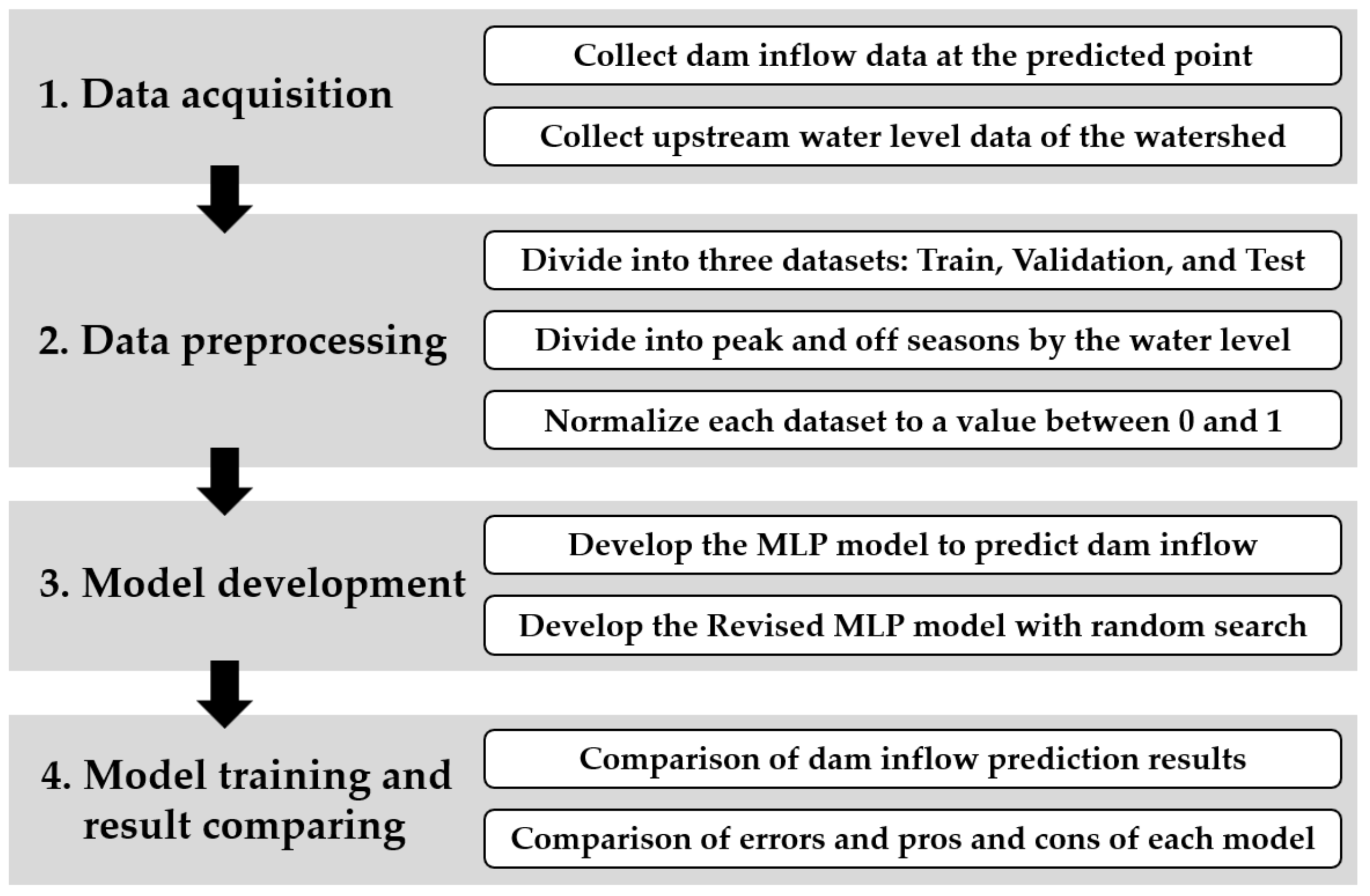
The study comprised four major stages. The first stage was the data-acquisition stage. The status of the target watershed was analyzed, and the required data point and period were selected. The second stage was data preprocessing. The acquired data were divided into training, validation, and test datasets, according to the measurement year. In this stage, two preprocessing steps were performed to improve the performance of the model. (1) Input data were divided into peak and off seasons and above- and below-average based on the water level gauge; (2) Input data were normalized to have a value between zero and one. Seasonal division and normalization were also performed. The third stage involved the construction of the MLP model to predict dam inflow. The analysis was performed for four scenarios: without preprocessing, seasonal division, normalization, and applying combined seasonal division and normalization. Next, an RMLP model with a random search algorithm was developed and analyzed in the same manner. Finally, the prediction results of the test datasets for the preprocessing and model improvement effects were compared. Figure 1 is a graphical overview representing the methodology of the study.
2.1. Data Preprocessing: Seasonal Division
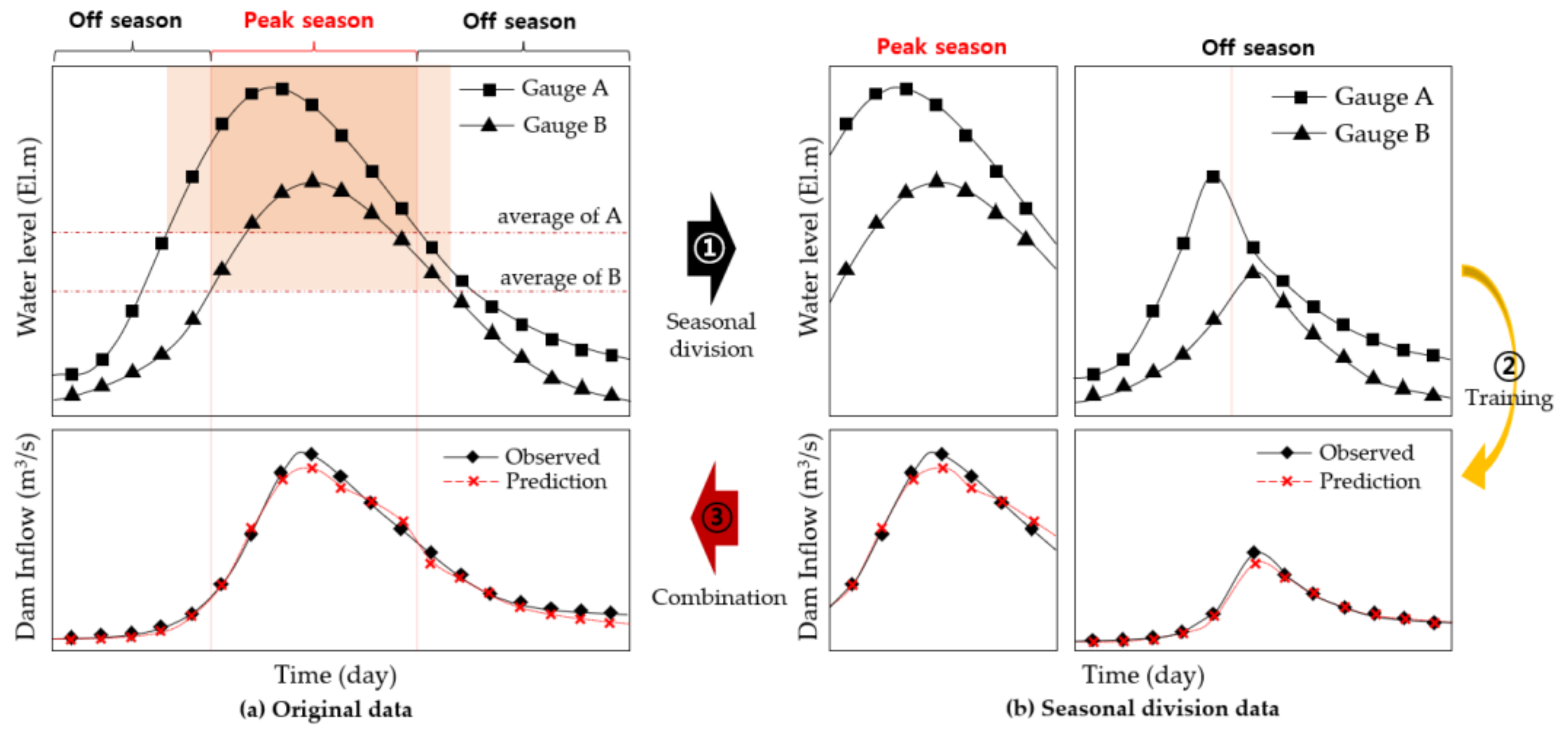
The water level and flow discharge were characterized by significant differences between the peak and off seasons. When rainfall occurred, the water level and flow discharge increased rapidly and then decreased over time. However, when no rainfall occurred, the water level and flow discharge were low because of the small base runoff. In South Korea, rainfall events are concentrated during the rainy season. Therefore, batch training the entire dataset results in a high possibility of decreased prediction accuracy during the peak season. To solve this problem, ① the input data were divided according to the upstream water level. The separation criterion was the average water level at the level gauge. In this study, two data points were used for the upstream water level. Peak season was defined when both water levels exceeded their average height, and all other conditions were defined as the off season, ② Model training was performed in the peak and off seasons, respectively, and ③ the two models were combined after the learning phase was completed. To verify the accuracy of the model, the discharge was predicted by dividing it into peak and off seasons based on the water level of the input data, and the model error and accuracy were calculated by combining the two results. The seasonal division process is briefly represented in Figure 2.
2.2. Data Preprocessing: Normalization
The data used for model training had different ranges and deviations, depending on the measurement point and type. When biased data were used as inputs to the model, biased results can be obtained during the training process of the model. To prevent this, all water level and discharge data were normalized between zero and one. This process was performed individually for the training, validation, and testing datasets. The data normalization process, called min-max scaling, was calculated using Equation (1).
where is the normalized data, is the original data without preprocessing, and are the minimum and maximum values, respectively, among the input data . This process made it possible to remove the bias due to the deviation of the data point characteristics.
2.3. Model Composition
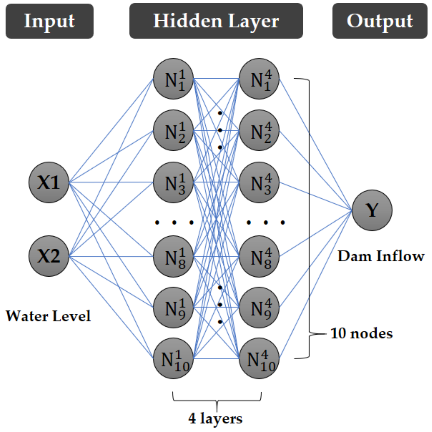
Except for their respective learning algorithm, the MLP and RMLP models have the same model and structure. The MLP model consisted of a dense structure, four hidden layers, and ten nodes per layer. There were two input nodes and one output node because the input data were the water level data of two locations, and the output datum was the predicted dam inflow. The activation function and optimizer of the model were the ReLu and Adam, respectively. The goal of the model training was to predict the average daily inflow of the dam through the upstream water level. Therefore, the daily average data were the temporal resolution. The model was written using Spyder (version 5.1.5), an open-source platform development environment based on the Python (version 3.8.12 64-bit) programming language. The structure of the model is shown in Figure 3.
Because the goal of this model was to approximate the inflow discharge, the mean squared error (MSE) was selected to calculate the error between the predicted model and the observed data. MSE is the average of the squares of the difference between the predicted and actual values. In general hydrology, the peak discharge during the peak season is more important than that during the off season. Therefore, an MSE that exaggerated the error in the peak discharge was selected. However, it depends on the scale of the data and has a weakness against data noise which is a disadvantage. Therefore, it is necessary to remove noise through data normalization.
2.4. Random Search Algorithm
The current MLP model calculates the gradient and performs weight updates using an optimizer. However, in this study, a new algorithm for updating the model weights is proposed. It adds two random searches (boundary and proportional random) to obtain smaller errors compared to the basic MLP model. The first step of the random search was “boundary random ()”, which was randomly changed within the range of the initial value of the weight. The random change was performed independently with the probability of the parameter for all weights in the model. The was calculated using Equation (2).
where is kth weight of the model, is random value between -one and one, is an initial boundary of model weight, is random value between zero and one for kth weight, and is the boundary random parameter and a preset value when constructing the model.
The second step was “proportional random ()”, which changed in proportion to the current weight value. In the method, the intensity of the weight change was assigned as a learning rate parameter (). The was calculated using Equation (3).
where is the learning rate, is the proportional random parameter. Both were determined when constructing the model.
A random search was performed with an independent probability for all the weights. If neither nor was selected, the original values were maintained. The sum of the probabilities of the two parameters did not exceed one. Setting the parameter value was important because it affected the analysis results. In this study, parametric sensitivity analysis was performed and = 0.05, = 0.01, and = 0.01 were set as optimal values.
2.5. Model Training Process
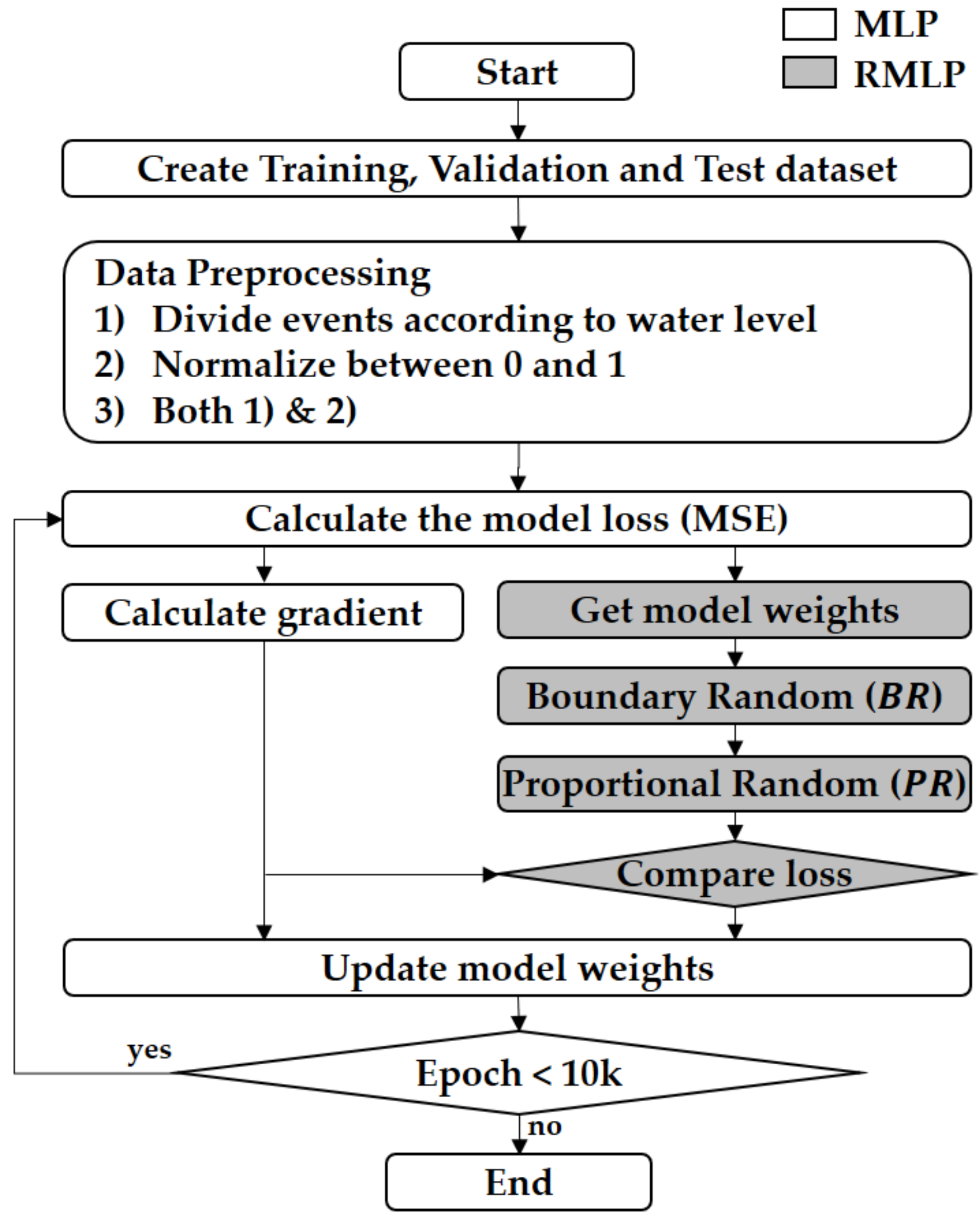
In the model training process, the MLP and RMLP followed a similar framework. First, the data were divided into training, validation, and testing datasets. In this study, daily data from 2004 to 2021 were used. Data from 2004 up to 2015 were classified as the training dataset, data from 2016 to 2018 as the validation dataset, and data from 2019 to 2021 as the test dataset. In the data preprocessing stage, based on the value of the upstream water level gauge, the dataset was (1) constructed by dividing it into above-average (peak season) and below-average (off season), (2) normalized to have a value between zero and one through min-max scaling, and (3) analyzed when preprocessing (seasonal division and normalization) was applied. The initial weight of the model also affected the learning performance. In this study, the initial boundary was set to 0.8 through sensitivity analysis. Accordingly, the initial weight of the model was randomly configured within the range of ±0.8. The initial loss for the original model without preprocessing was calculated as MSE, and the weight update was performed by calculating the gradient of the loss. For the weight update, the current method (MLP) and the new algorithm (RMLP) were applied. In RMLP, before updating the weights, the results derived from the random search were compared with the results of MLP using the current optimizer, and the more accurate weights were transferred to the next epoch. If the random search result was worse than the current optimizer result, the next epoch was performed using the current optimizer result. Thus, better alternatives were selected, resulting in more effective results compared to the existing model. This process was repeated from the MSE calculation until the number of epochs exceeded 100,000. The learning process of the model is illustrated in Figure 4.
In general, the training error continuously decreased as the epoch progressed. However, the validation error may show a different pattern. This problem called overfitting occurred because the model training data are limited. To solve the overfitting problem, the validation error was continuously tracked during the learning process, and the result with the smallest validation error was selected as the final model. In the learning process, the validation error was analyzed by repeating 20 epochs up to 100,000 times.
3. Application and Results
3.1. Target Area
The target watershed was the Soyang Dam Basin, located in Gangwon-do, South Korea, as shown in Figure 5. The area of the basin was 2694.4 km2, the basin circumference was 383.6 km2, the average width of the basin was 16.5 km, and the average watershed slope was 46.0% [37]. The flow discharge into the Soyang Dam was generated from the Inbukcheon and Soyang rivers. The Soyang Dam was built at the exit of the basin with a storage capacity of 2.9 billion tons. Daily average water level data from 2004 to 2021 were acquired from two water gauges (Wontong and Wondae) installed in Inbukcheon and Soyang rivers, respectively. The daily average dam inflow data for the same period was investigated to determine the water level-inflow discharge time series data.
3.2. Preparation of Input Data
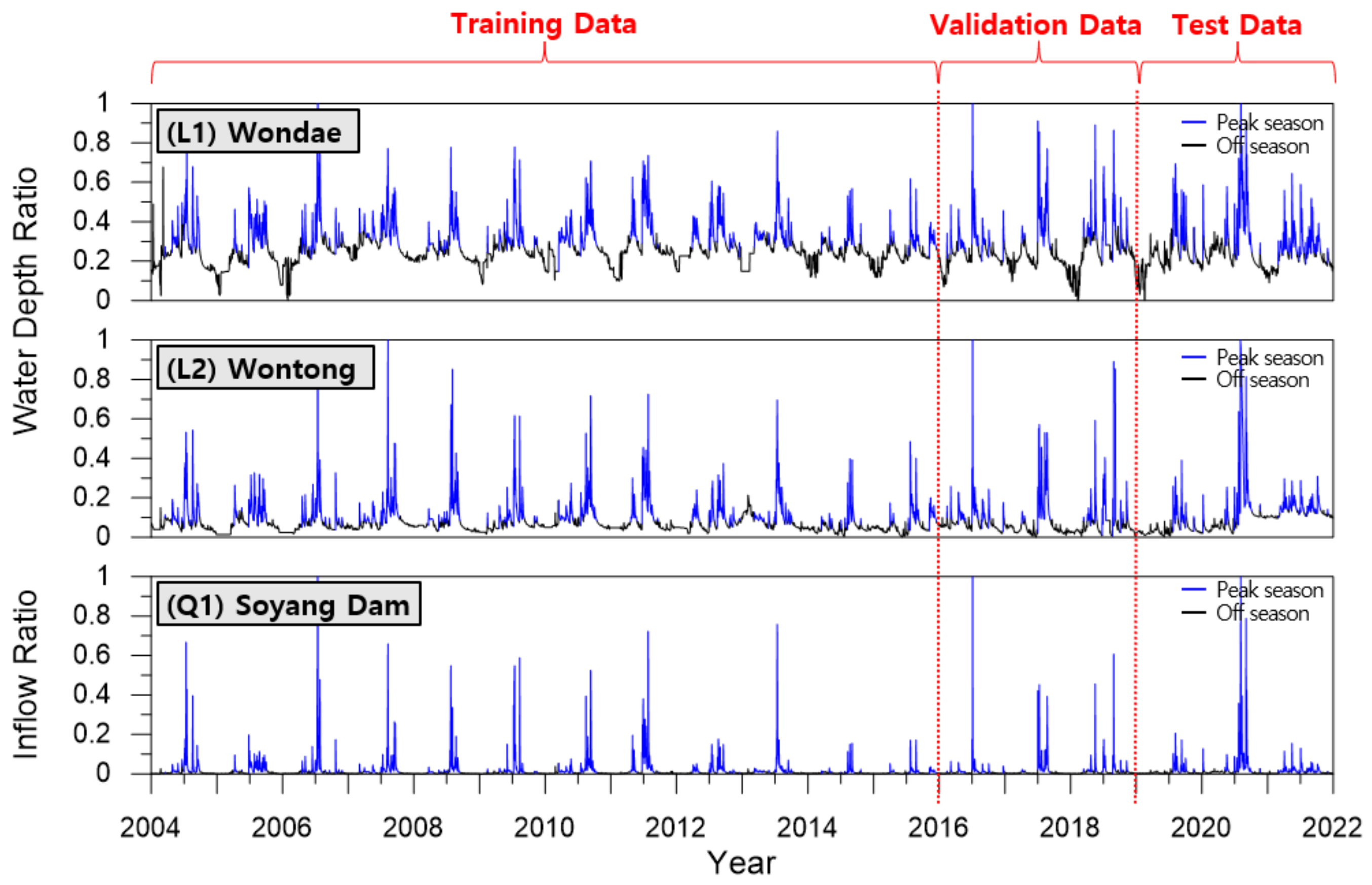
Data from two water gauges located in the middle and upstream of the Soyang Dam Basin and the dam inflow were used as training data for the prediction model. The daily average data from 2004 to 2021 were provided by the Water Resource Management Information System (WAMIS) [38]. Data preprocessing was performed to build the training, validation, and test models. A total of 4383 data points from 2004 to 2015 were used as the training dataset, 1096 data points from 2016 to 2018 were used as the validation dataset, and the remaining 1096 data points from 2019 to 2021 were used as the test dataset. The cases where both the Wondae and Wontong water levels were above average were classified as the peak season, and the other cases were classified as the off season. The total number of days corresponding to the peak season was 1717, including the 1183 days of training data, 240 days of validation data, and 294 days of test data. The off season was 4858 days long, comprising 3200 days of training data, 856 days of validation data, and 802 days of test data. The number of each dataset and its maximum and minimum values are listed in Table 1 and Table 2.
The entire dataset had two sets of water level data and one set of dam inflow data. This was further divided into training, validation, and test data according to the measurement year. The peak season (blue line) and off season (black line) were differentiated according to the water level. Seasonal changes in the water level and inflow discharge were clearly visible. The inflow discharge was closer to zero during the off season and showed a large difference between annual peak seasons. Therefore, more accurate prediction results could be obtained by training the model and dividing the peak and off seasons. The entire input dataset is presented as a time-series graph, as shown in Figure 6.
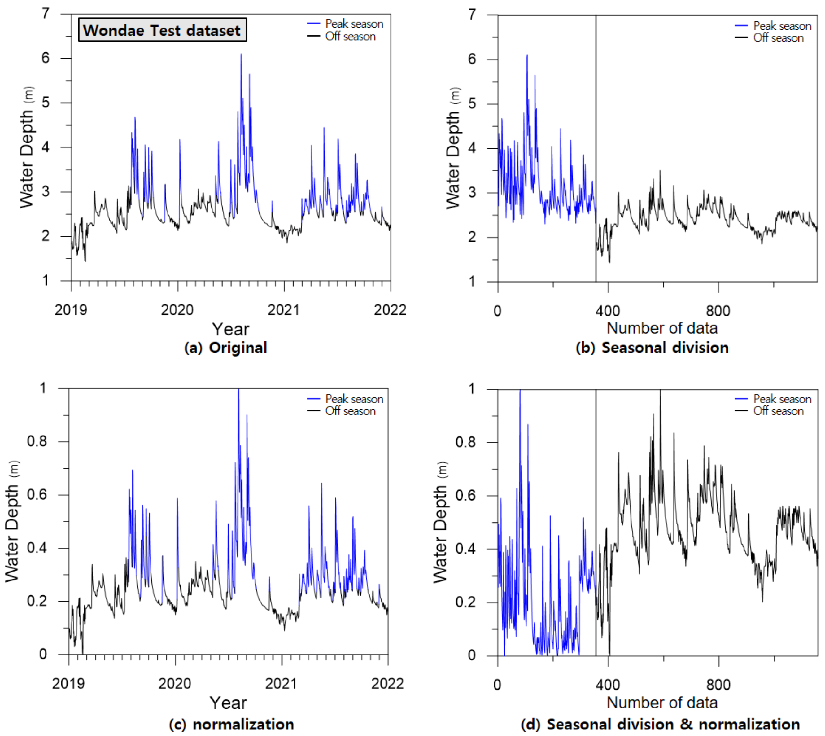
Figure 7 shows the input data separated according to the type of preprocessing, using the Wondae gauge dataset as an example.
Four types of preprocessing methods were applied to the MLP and RMLP models. Figure 7a shows the original data without preprocessing. The blue line corresponds to the peak season, and the black line corresponds to the off season, which was used as learning data, as shown in Figure 7b. Figure 7c shows the data normalized to between zero and one, and Figure 7d shows the data that applies both seasonal division and normalization.
In this study, eight cases were classified according to the model and preprocessing types. In the MLP model, Case 1 (without preprocessing), Case 2 (seasonal division), Case 3 (data normalization), and Case 4 (both seasonal division and normalization) were applied. Similarly, the RMLP model was classified from Cases 5 to 8. The total cases are presented in Table 3.
3.3. Model Parameter Estimations for MLP and RMLP
Because model parameters affected the performance of the MLP and RMLP models, it was important to set appropriate values. Each model required different parameters. In the MLP model, the range of the initial weights () should be set. This value was used when building the model initially and was not involved in the subsequent learning process. However, in the gradient descent, the initial value was important because it affected the overall learning result. In this study, the model parameters were determined through parameter sensitivity analysis. The results were compared by setting the range of the initial weight in four steps: 0.2, 0.4, 0.6, and 0.8. After training the model, the test dataset was used to compare the MSE with the smallest value. The analysis was repeated ten times, and 10,000 epochs were analyzed during each analysis cycle. The average and minimum values of the test error for each parameter were analyzed, as shown in Table 4. Finally, the MLP model parameter was determined to be = 0.8 with the smallest mean and minimum errors.
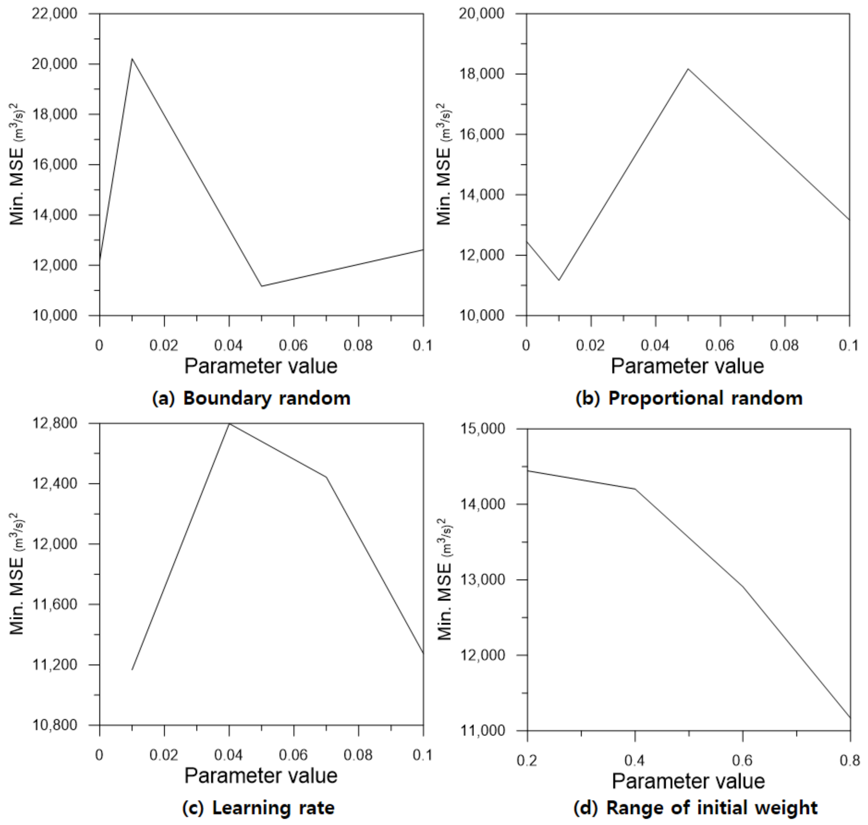
In the RMLP model, four parameters were set. The and parameters represented the probability of performing each random search with a value between zero and one. The sum of these two probabilities did not exceed one. A sensitivity analysis of the two parameters was performed for four cases: 0.0, 0.01, 0.05, and 0.1. The learning rate () indicated the strength of the existing weight values when was applied. Sensitivity analysis was performed using four values: 0.01, 0.04, 0.07, and 0.1. Finally, the range of the initial weight was analyzed using four values: 0.2, 0.4, 0.6, and 0.8. Unlike that in MLP, when applying , the range of the initial weight must be considered continuously. In this study, assuming a small learning rate effect, was fixed at 0.01, and then the analysis was performed ten times for all 64 cases configurable with the remaining three parameters: , , and . The test error had minimum values at = 0.05, = 0.01, and = 0.8. Subsequently, the three parameters were fixed, and sensitivity analysis of the learning rate was performed to obtain a minimum error at = 0.01. Finally, the RMLP model parameters were determined as = 0.05, = 0.01, = 0.01, and = 0.8. Table 5 presents the sensitivity analysis results for the RMLP model parameters.
As a result, except for the case of zero (without ), the error decreased and then increased in a concave shape and was the smallest at = 0.05. Conversely, showed a convex shape and had the highest accuracy at = 0.01, the minimum value excluding zero (without ). The learning rate showed a convex shape, with a minimum error at = 0.1. In both MLP and RMLP, the model accuracy improved as the range of initial weight increased. The model accuracy according to the change of each parameter is shown in Figure 8.
The parameters of the MLP and RMLP models were determined through parameter sensitivity analysis, as shown in Table 6.
In the MLP model, the range of the initial weight value () was set to 0.8. In the RMLP model, the parameter was 0.05, parameter was 0.01, learning rate () was 0.01, and the range of initial weight () was set to 0.8, the same as in the MLP model.
3.4. Data Preprocessing Results
For the analysis of the preprocessing effect of the input data in the MLP and RMLP models, learning for eight cases was performed using four types of input data and two models. The analysis was repeated 20 times and was performed for up to 10,000 epochs during each cycle. Training and validation errors were calculated for each epoch, and the model with the smallest validation error was selected as the final model. The performance of the model is shown in Table 7 as MSE for the test data.
In the MLP model, the test error of the inflow prediction result without preprocessing (Case 1) was 11,006. When dividing the peak season and off season (Case 2), it was 14,370, which was an increase of 3364 (30.6%). When data normalization was performed (Case 3), MSE was 8985, which was reduced by 2021 (18.4%) compared to that of Case 1. The result of applying both preprocessing steps (Case 4) was 4511, which decreased by 6495 (59.0%) compared to that of Case 1. All results with normalization showed better results than those of Case 1 because normalization reduced the error caused by the deviation of the training data. In contrast, when only seasonal division was applied, the error increased compared to the original results without preprocessing. Owing to flood characteristics in South Korea, the difference between the peak and off seasons was large, and the low discharge was close to zero. When the discharge was small, the MSE was relatively small, even if an error occurred. When the discharge was large, MSE became large because the square of the deviation increased, while the amount of data was small. The error was the smallest when both preprocessing techniques were applied. Therefore, normalization must be applied with seasonal division. The instability that occurred in the peak season model was reduced through the normalization process. Consequently, the prediction accuracy of the combined peak and off seasons was significantly improved when both preprocessing methods were applied.
The results of the RMLP model analysis showed similar patterns. For the discharge prediction without preprocessing (Case 5), the test error was 11,344. When analyzed by dividing the peak and off seasons (Case 6), the MSE was 12,251, which increased by 907 (8.0%) compared to that in Case 5. After data normalization (Case 7), the MSE decreased from 5978 (52.7%) to 5366. When both preprocessing steps were applied, the MSE was 4368, which is 6976 (61.5%) less than the MSE of Case 5. As with the MLP results, applying both preprocessing methods was more effective than only applying the normalization method.
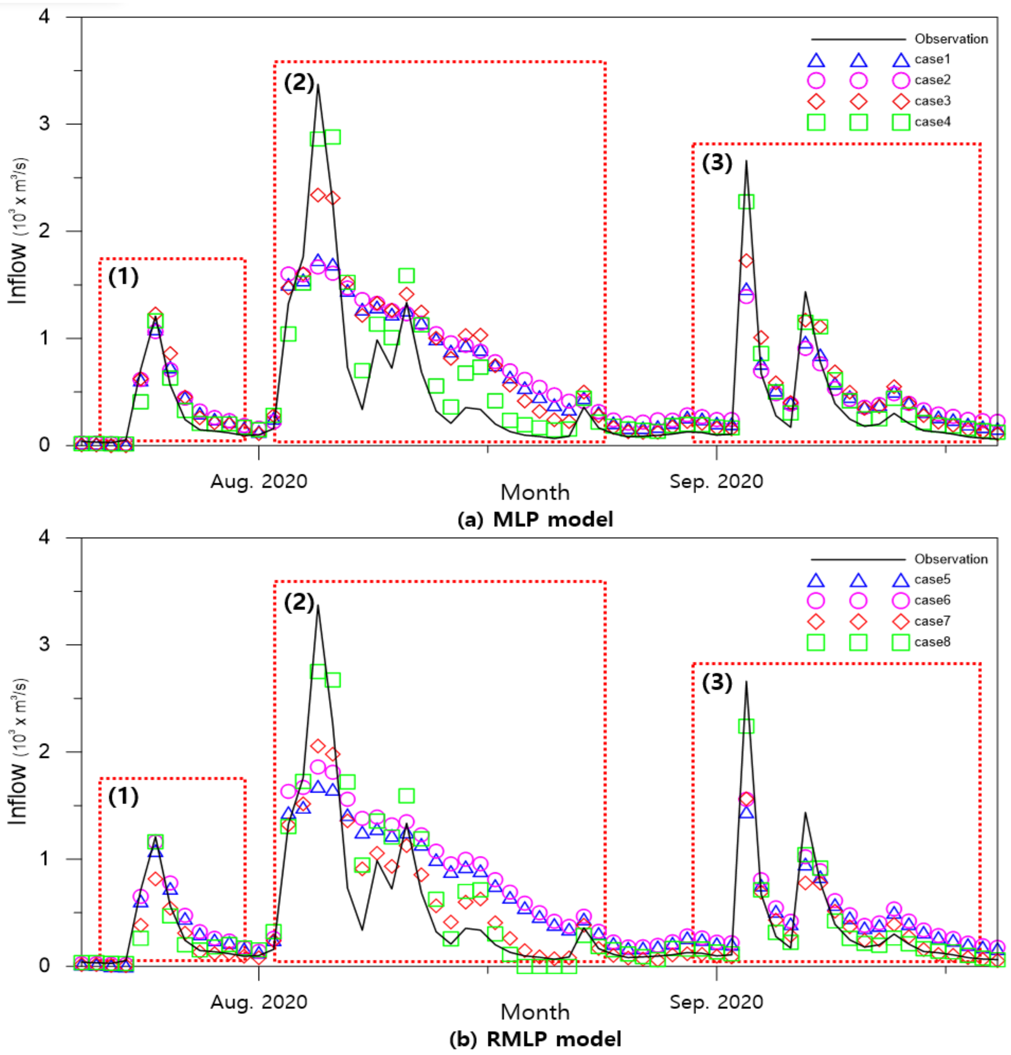
The difference between the measured flow rate and the predicted value was compared using a diagram. The analysis was centered on July–September 2020, when the largest flow occurred among the test datasets. Figure 9 shows the measured flow discharge and the prediction results of Cases 1–4 using the MLP and Cases 5–8 using the RMLP models.
This graph indicates that three major flood events occurred in 2020. There was a single peak event at (1), multiple smaller peak events, the largest event at (2), and two more peak events at (3). In case (1), the peak discharge was small, and the hydrograph only changed slightly. The preprocessing and model improvement results were not significantly different, and both were predicted relatively accurately. When data preprocessing was not used (Case 1), or only seasonal division was used (Case 2), the peak was underestimated, and the accuracy of the flow reduction curve was poor. The results with normalization (Case 3) predicted a relatively accurate peak discharge, and there was a minor improvement in the low discharge. When applying both seasonal division and normalization (Case 4), peak discharge, flow reduction patterns, and subsequent peaks were predicted accurately. Although the peak discharge was underestimated, the accuracy of the flow-reduction curve was significantly improved. A hydrograph with a rapid increase was observed, with two peaks at (3). Similar to the previous results, there was a slight improvement in the peak prediction for Case 3, and the most accurate peak was the result for Case 4.
The RMLP model predicted the peak and flow reduction curve as well as the MLP at (1). However, it showed a noticeable accuracy improvement at (2), especially in Case 7, compared to Case 3. When only data normalization was applied in Case 7, there was a significant improvement in the prediction accuracy of the flow reduction curve. Consequently, the MSE was smaller in Case 7 than in Case 3. Peak and low discharge predictions were significantly improved in Case 8 in which seasonal division and data preprocessing were applied together. (3) is a hydrograph with a rapid increase and two peaks. Similar to previous results, Case 8 was the most accurate prediction.
As a result of data preprocessing, there was a tendency to underestimate the peak discharge. The reason for this error is the limitation of the error calculation algorithm. Owing to the relatively short duration of peak flooding, the amount of high-flow data was small. In this study, the amount of off season data was more than twice that of the peak season. Therefore, the learning direction was focused on abandoning the peak error and reducing the low flow error, which is a common problem in algorithms that calculate average error. To reduce this error, the peak and off seasons were separated. However, if the discharge were simply separated, the fluctuation in the peak season would still be high. As a result, the error increased, as in Cases 2 and 6. Because the variation in the peak season was larger than that in the off season, data normalization was necessary to improve the accuracy. Data normalization converted the discharge to a value between zero and one, to limit the fluctuation range of the peak season and improve the learning accuracy. Both high and low discharges can be accurately predicted by performing both preprocesses.
3.5. Model Comparison
In this study, the RMLP model was proposed for accurate discharge prediction, which improved the learning algorithm and data preprocessing methods of the model. The RMLP model was more accurate than the MLP model. When using existing data without data preprocessing (a), the test error increased by 338 (3.1%) from 11,006 to 11,344 in the MLP model. However, the difference was not significant because the basic error value was large. Seasonal division (b) decreased by 2119 (14.7%) from 14,370 to 12,251. In both cases, the error increased. This problem occurred because the increase in MSE at high flow was larger than the decrease in MSE at low flow. Because the amount of high flow data was small and the data deviation was large, the MSE result was larger than that of (a). Nevertheless, the error increase rate was relatively small in the case of the RMLP model. To solve this problem, data normalization was required. As a result of data normalization, the MSE decreased by 3619 (40.3%) from 8985 to 5366. There was a relatively low error in Case 7 when only data normalization was used in RMLP, and the model improvement was the most prominent. When both preprocessing steps were performed, the MSE decreased by 142 (3.1%) from 4511 to 4368. Except for Cases 1 and 5, RMLP exhibited better results than MLP. The model improvement effect is quantitatively expressed in Table 8.
Note that a small test error does not always mean the performance of the learning algorithm is good. In this study, the model showed that the minimum validation MSE was selected during the epochs, as explained in Section 2.5. Because the RMLP model had a better learning performance than the MLP model, the minimum validation MSE was smaller among the results which were repeated 20 times. However, the training caused an overfitting problem because it only considered the validation data. As new data are input, prediction accuracy may decrease. To solve this problem, prediction performance should be measured using new data. The final MLP and RMLP models were chosen to have the smallest test MSE among the 20 results. However, the test MSE only demonstrated the prediction accuracy of the model and had no effect on the model training performance. Even if the global minimum of the validation MSE was found using a new algorithm with excellent learning ability, the test MSE may be worse than that of the basic MLP model. Therefore, the overall test error can be smaller in RMLP but not always.
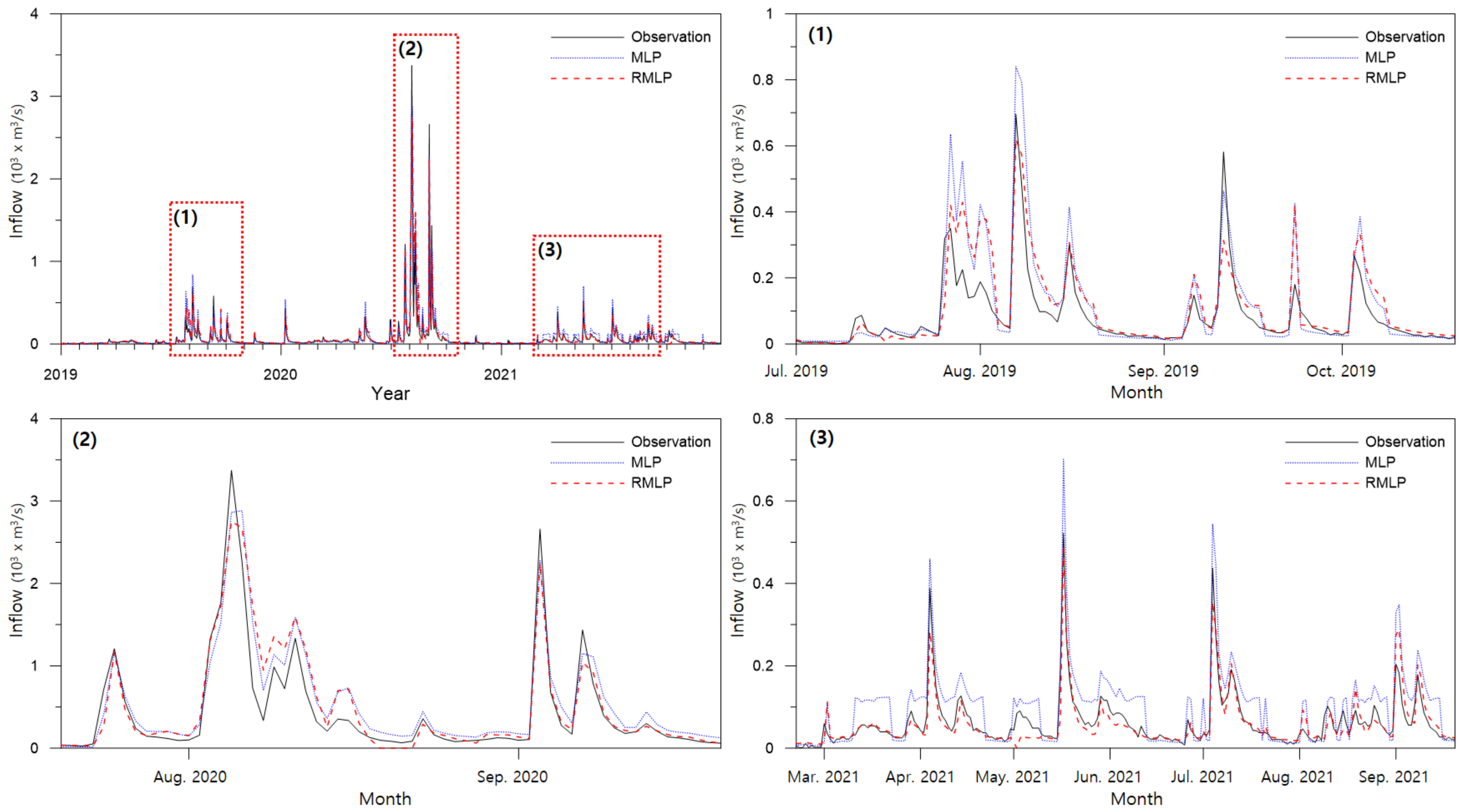
To analyze the model improvement effect, the final MLP and RMLP models (Cases 4 and 8, respectively) were compared using a time series graph. Preprocessing method (d) was applied to both models, and the test data were predicted. Figure 10 compares the measured discharge for the entire test dataset with the predicted values of the two models. During the entire period, major flood events by year are indicated as Events (1) to (3) and expanded using a higher resolution. Event (1) displayed a tendency to overestimate MLP and partially underestimate RMLP in the peak flood forecast based on the 2019 inflow hydrograph analysis. At a low discharge in Event (1), both models provided similar results. Event (2) showed the largest peak value of the hydrologic curve in 2020. The peak prediction tended to be underestimated, and MLP was closest to the observation data, showing a larger peak than RMLP. Event (3) was the case in which low volume rainfall occurred continuously. Again, MLP was overestimated compared to RMLP and showed an unstable overestimation at mid-low discharges. RMLP predicted a more accurate hydrograph at low and medium discharges. Overall, MLP showed a tendency to overestimate discharge, and the accuracy of RMLP was confirmed to be better in the overall hydrograph prediction.
To quantify the difference in peak discharge, the three largest peaks were selected for each year, and the discharge error was compared. In 2020, the largest peak was 3373.1 m3/s. The MLP model predicted 2862.9 m3/s, which was underestimated by 510.2 m3/s (15.1%), and the RMLP model predicted 2752.0 m3/s, which was 620.7 m3/s (18.4%). MLP was more accurate when only considering the largest peak value. However, when considering all nine peaks, RMLP showed a smaller error. MLP showed a mean deviation of 237.6 m3/s (26.3%), and RMLP showed 187.4 m3/s (12.1%). Again, the MLP tended to overestimate the peak value. In conclusion, the RMLP model can predict the amount of dam inflow more accurately in most cases. Table 9 shows the forecast results for major peak events by year.
In this study, the model was trained to minimize the validation MSE, and the final model was selected to minimize the test MSE. Because MSE reflects the error of the entire time series, the accuracy of the model cannot be judged only through the difference in several peak flood errors. In Table 9, the RMLP shows a smaller error when averaging the error of nine peaks, but the MLP shows more accurate results in the largest peak discharge. A decision based on the purpose of the predictive model is necessary. If the model is required to predict the peak flow close to the existing maximum flood, a suitable model learning algorithm is needed. This study only considered the MSE of the model, but results may be derived by additionally considering the error of the peak flow in learning. Future studies may consider multi-purpose model learning, however, the current study focused on improving the model’s learning algorithm and analyzing the preprocessing effect.
4. Discussion
In this study, MSE was used for error calculation in model training. MSE computes the square of the error difference. Therefore, the errors at large values tend to be overestimated. This phenomenon caused a larger error when the model was trained by dividing it into high discharge and low discharge in Cases 2 and 6. As shown in Table 10, the basic MSE of the RMLP model (Case 5) was 11,344, but the MSE of the seasonal division model during the peak season was 45,417, which increased significantly by 33,773 (297.1%). In the off season, MSE significantly decreased by 11,248 (99.2%) to 96 combined with relatively small fluctuations in discharge. Combining these results, the final MSE was 12,251, which was 907 (8.0%) larger than the original data value. The phenomenon when the error significantly depends on the size of the value can occur even after normalization. The normalization (Case 6) MSE increased by 10,700 (199.4%) from 5366 to 16,066 during the peak season and decreased by 5286 (98.5%) from 5366 to 80 during the off season, resulting in a final MSE of 4368, which decreased by 998 (18.6%). In both cases, the MSE in the peak season increased and the MSE in the off season decreased significantly. However, the error increase without normalization was greater than that of the error-reduction effect. To confirm this difference more intuitively, the mean absolute error (MAE) was calculated and displayed. Similarly, for MAE, it was confirmed that the error in the peak season was large, and the error in the off season was small.
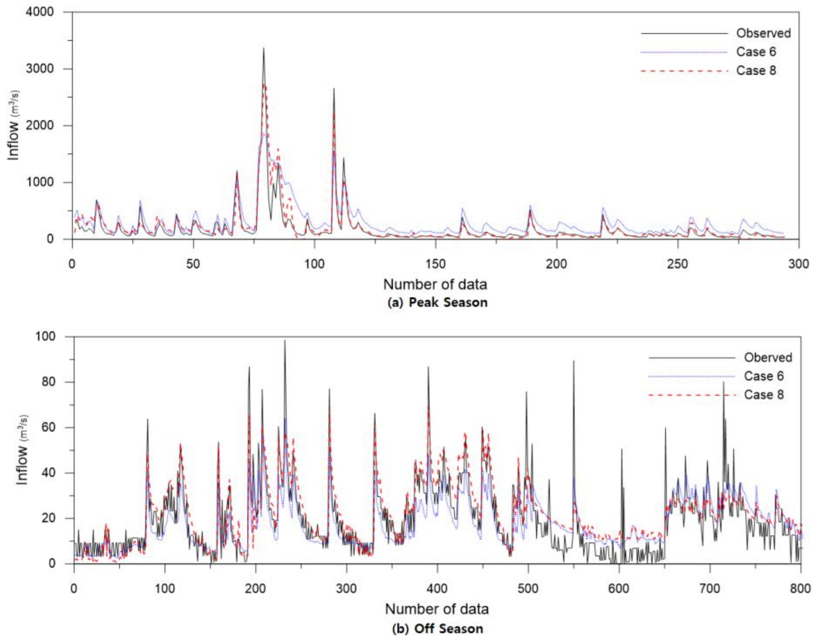
The discharge prediction results in Cases 6 and 8 in which seasonal division was performed, were compared, as shown in Figure 11. It shows the measured discharge and predicted values on a log scale during the peak (a) and off (b) seasons.
Compared to the measured values, the predicted values in (a) Case 6 were overestimated, and Case 8 was relatively accurate. (b) was the discharge prediction result in the off season and was predicted almost accurately at 10 m3/s or more. There were some inconsistencies in the low discharge values of 10 m3/s or less. However, the MSE was also small because the discharge values and differences were small. As a result, there was still an underestimation error, the MSE of Case 8 in the off season was 80, which was smaller by 16 compared to that of Case 6. When applying seasonal separation, improvement in the prediction accuracy of medium to high flow is important. However, there was no significant difference in the accuracy at low flow rates, even with some errors. Therefore, to improve the accuracy of the high flow prediction model, further study to separate the high flow into two or more stages, such as high, medium high, and low, should be conducted.
Finally, the MSE, root mean squared error (RMSE), MAE, sum of absolute difference (SAD), mean absolute percentage error (MAPE), coefficient of determination (R2), and coefficient of efficiency (E) were analyzed. Each of the equations is given in Appendix A. In this study, MSE was used as an error calculation method, but MAE also showed a similar tendency to MSE. However, MAE was not suitable for use as an evaluation index for model learning because it showed fewer error values compared to MSE. In addition, because there was no error weight for the high and low flows, it was easy to obtain a result that was biased toward low flow with a large amount of data. Therefore, for discharge prediction, the MSE is more appropriate than the MAE. The results for all the cases are shown in Table 11.
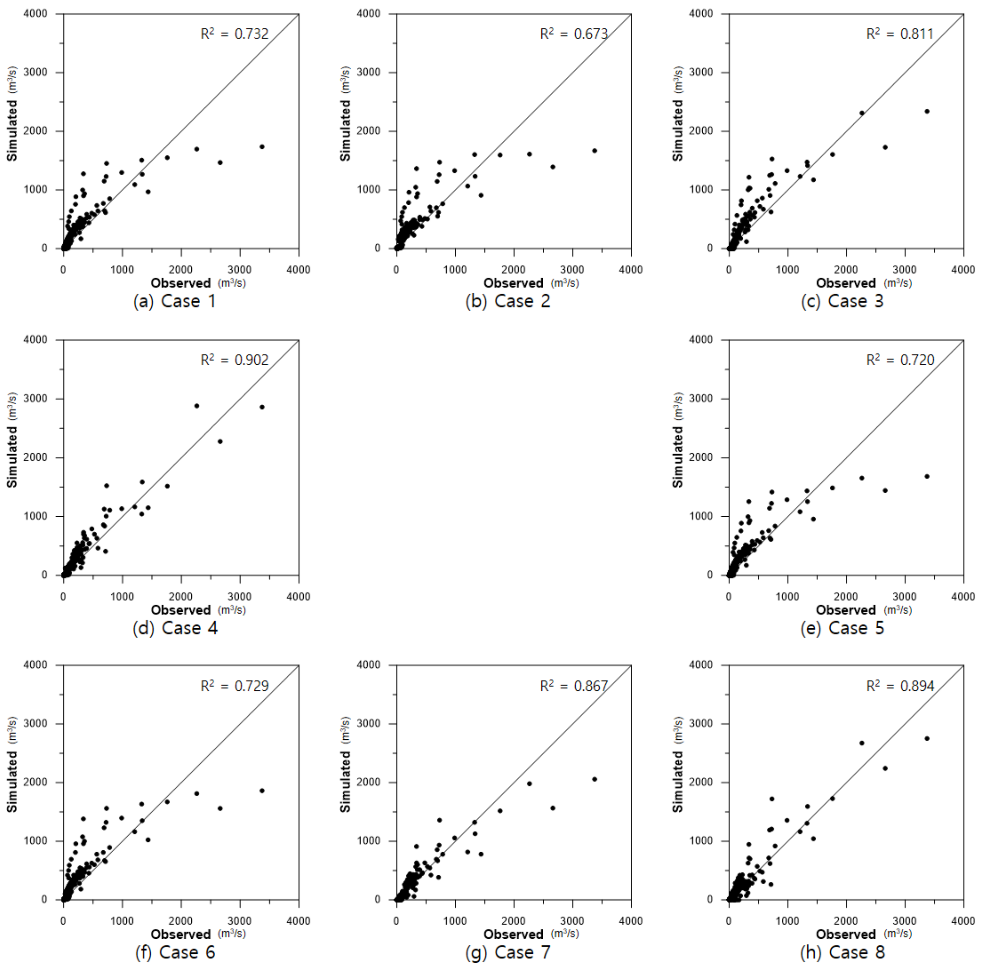
Additionally, without preprocessing or seasonal division alone, R2 showed an accuracy of approximately 0.7, and the high discharge was underestimated. In cases where only normalization preprocessing was performed, such as in Cases 3 and 7, R2 was significantly improved. In MLP (Case 3), the medium-low discharge was overestimated, but in RMLP (Case 7), it was significantly improved, and the R2 also increased from 0.811 to 0.867. Finally, when all preprocessing steps were applied, both MLP (Case 4) and RMLP (Case 8) showed an accuracy close to 90%. The R2 for the measured and predicted discharges for each model are shown in Figure 12.
With the dam inflow prediction model developed in this study, it is possible to predict in advance the dam inflow according to the change in the upstream water level. By measuring water stored in the dam and the predicted inflow, it is possible to set an operation rule to secure the water storage during the dry season or to secure the dam reserve by discharging it in advance during the flood season.
5. Conclusions
This study aimed to develop an inflow prediction model for stable dam operation in the Soyang Dam Basin. Inflow prediction was performed using an MLP model. Two approaches were used to increase prediction accuracy. First, the learning accuracy was increased by preprocessing the input data. For preprocessing, two methods were used: Dividing the learning data into the peak and off seasons and normalizing the input data to reduce the deviation of the data. Second, the learning algorithm of the MLP model was improved. A previous MLP used gradient descent to train the model. In this study, a random search algorithm was applied to the existing MLP model such that a wider range of alternatives could be found when the model weight was updated.
The MLP model of the dense structure was used for model construction. Four hidden layers were used with ten nodes per layer. ReLu was used as the activation function, and Adam was used as the optimizer. MSE was used for the error calculation for model training, and MAE and R2 analyses were performed. The input data for model learning were the water level and dam inflow data provided by WAMIS. The study area was the Soyang Dam Basin, and time series data were used for 6575 data points from 2004 to 2021. Training was repeated 20 times every 10,000 epochs to determine the final model weights.
As a result of the model training, it was possible to reduce the error by up to 6976 (61.5%) from MSE of 11,344 to 4368 through data preprocessing. During model training, the error increased when learning by dividing the peak and off seasons. This error occurred excessively owing to the large deviation in the peak data. However, when seasonal division was performed with data normalization, the error owing to the size of the deviation was reduced, enabling high-accuracy learning. The RMLP model showed the greatest improvement effect compared to the MLP model in Case 7, which was reduced by 3619 (40.3%) from 8985 MSE to 5366 MSE. When all preprocessing steps were performed (Case 8), the error reduction rate was small, but an error of 4368 was obtained, which was improved by 142 (3.2%) compared to the MLP error of 4511. Comparing the hydrographs of both models, MLP showed a tendency to overestimate high and intermediate flows, but RMLP predicted the overall hydrograph more accurately. The prediction accuracy of the final RMLP model was MSE 4368, MAE 21.9, peak discharge error 12.1%, and R2 = 0.894.
This model enables high-accuracy inflow forecasting throughout the peak and off seasons and will help in the efficient operation of the dam and ensure safety by predicting the inflow through the upstream water level. A limitation of this study is that it is difficult to guarantee the accuracy of the model when the flooding is greater than the past maximum peak. Therefore, it is essential to continuously measure the data and supplement the model to improve the prediction accuracy, even after the model is derived. In addition, this study was limited to the Soyang dam basin. It is necessary to apply the learning model to different watersheds or apply the learning model to various objects such as the groundwater level, storm water pipe system, and other time series data. In follow-up studies, seasonal divisions will be further subdivided to improve the prediction accuracy at high discharge. In addition, a study to improve the learning algorithm of time-series prediction models such as RNN or LSTM and compare it with MLP will be conducted. It is expected that more accurate prediction models and algorithms can be developed by continuously improving hydraulic and hydrologic prediction models.
Author Contributions
H.S.C. and E.H.L. conducted the literature review. H.S.C. drafted the manuscript. H.S.C. worked on subsequent manuscript drafts. H.S.C. performed simulations. H.S.C., S.-K.Y., J.H.K. and E.H.L. conceptualized the proposed method. All authors have read and agreed to the published version of the manuscript.
Funding
This study was funded by the Seoul Institute of Technology (SIT) (2021-AB-007).
Institutional Review Board Statement
Not applicable.
Informed Consent Statement
Not applicable.
Data Availability Statement
The data that support the findings of this study are openly available in Water Resources Management Information System at http://www.wamis.go.kr/ (accessed on 5 March 2022) reference number [38]. The program code is available at https://doi.org/10.24433/CO.7415800.v1 (accessed on 31 May 2022).
Acknowledgments
This work was supported by grants from the Seoul Institute of Technology (SIT) (2021-AB-007) and the National Research Foundation (NRF) of Korea (NRF-2019R1I1A3A01059929).
Conflicts of Interest
The authors declare no conflict of interest.
Appendix A
To compare the accuracy of MLP and RMLP models, mean squared error (MSE), root mean squared error (RMSE), mean absolute error (MAE), mean absolute percentage error (MAPE), sum of the relative error (SRE), coefficient of determination (R2), and coefficient of efficiency (E) were applied. The MSE equation is given by Equation (A1).
where is the observed inflow, is the predicted inflow, and n is the number of data. The RMSE equation is shown in Equation (A2) [33].
The MAE equation is shown in Equation (A3).
The SAD equation is shown in Equation (A4) [35].
The MAPE equation is shown in Equation (A5) [36].
The R2 equation is shown in Equation (A6).
where is the average observed inflow. The E equation is shown in Equation (A7) [34].
References
- McCulloch, W.S.; Pitts, W. A Logical Calculus of the Ideas Immanent in Nervous Activity. Bull. Math. Biophys. 1943, 5, 115–133. [Google Scholar] [CrossRef]
- Rosenblatt, F. The Perceptron: A Probabilistic Model for Information Storage and Organization in the Brain. Psychol. Rev. 1958, 65, 386–408. [Google Scholar] [CrossRef] [PubMed]
- Rumelhart, D.E.; Hinton, G.E.; Williams, R.J. Learning Representations by Back-Propagating Errors. Nature 1986, 323, 533–536. [Google Scholar] [CrossRef]
- Lecun, Y.; Bottou, L.; Bengio, Y.; Haffner, P. Gradient-Based Learning Applied to Document Recognition. Proc. IEEE 1998, 86, 2278–2324. [Google Scholar] [CrossRef]
- Hochreiter, S.; Schmidhuber, J. Long Short-Term Memory. Neural Comput. 1997, 9, 1735–1780. [Google Scholar] [CrossRef]
- Chung, J.; Gulcehre, C.; Cho, K.; Bengio, Y. Empirical Evaluation of Gated Recurrent Neural Networks on Sequence Modeling. arXiv 2014, arXiv:1412.3555. [Google Scholar]
- Hinton, G.E.; Srivastava, N.; Krizhevsky, A.; Sutskever, I.; Salakhutdinov, R.R. Improving Neural Networks by Preventing Co-Adaptation of Feature Detectors. arXiv 2012, arXiv:1207.0580. [Google Scholar]
- Hahnloser, R.H.; Seung, H.S.; Slotine, J.J. Permitted and Forbidden Sets in Symmetric Threshold-Linear Networks. Neural Comput. 2003, 15, 621–638. [Google Scholar] [CrossRef]
- Nair, V.; Hinton, G.E. Rectified Linear Units Improve Restricted Boltzmann Machines. In Proceedings of the 27th International Conference on Machine Learning, Haifa, Israel, 21–24 June 2010; pp. 807–814. [Google Scholar]
- Maas, A.L.; Hannun, A.Y.; Ng, A.Y. Rectifier Nonlinearities Improve Neural Network Acoustic Models. In Proceedings of the 30th International Conference on Machine Learning, ICML 2013, Atlanta, GA, USA, 21–24 June 2013. [Google Scholar]
- Riedmiller, M.; Braun, H. Rprop-A Fast Adaptive Learning Algorithm. In Proceedings of the ISCIS VII, Antalya, Turkey, 2 November 1992. [Google Scholar]
- Duchi, J.; Hazan, E.; Singer, Y. Adaptive Subgradient Methods for Online Learning and Stochastic Optimization. J. Mach. Learn. Res. 2011, 12, 2121–2159. [Google Scholar]
- Hinton, G.; Srivastava, N.; Swersky, K. Neural Networks for Machine Learning lecture 6a Overview of Mini-Batch Gradient Descent. Cited 2012, 14, 2. [Google Scholar]
- Kingma, D.P.; Ba, J. Adam: A Method for Stochastic Optimization. arXiv 2014, arXiv:1412.6980. [Google Scholar]
- Sit, M.; Demiray, B.Z.; Xiang, Z.; Ewing, G.J.; Sermet, Y.; Demir, I. A Comprehensive Review of Deep Learning Applications in Hydrology and Water Resources. Water Sci. Technol. 2020, 82, 2635–2670. [Google Scholar] [CrossRef]
- Tran, Q.-K.; Song, S.-K. Water Level Forecasting Based on Deep Learning: A Use Case of Trinity River-Texas-The United States. J. KIISE 2017, 44, 607–612. [Google Scholar] [CrossRef]
- Hu, C.; Wu, Q.; Li, H.; Jian, S.; Li, N.; Lou, Z. Deep Learning with a Long Short-Term Memory Networks Approach for Rainfall-Runoff Simulation. Water 2018, 10, 1543. [Google Scholar] [CrossRef]
- Kratzert, F.; Klotz, D.; Brenner, C.; Schulz, K.; Herrnegger, M. Rainfall–Runoff Modelling Using Long Short-Term Memory (LSTM) Networks. Hydrol. Earth Syst. Sci. 2018, 22, 6005–6022. [Google Scholar] [CrossRef]
- Jung, S.; Cho, H.; Kim, J.; Lee, G. Prediction of Water Level in a Tidal River Using a Deep-Learning Based LSTM Model. J. Korea Water Resour. Assoc. 2018, 51, 1207–1216. [Google Scholar] [CrossRef]
- Yuan, X.; Chen, C.; Lei, X.; Yuan, Y.; Muhammad Adnan, R. Monthly Runoff Forecasting Based on LSTM–ALO Model. Stoch. Environ. Res. Risk Assess. 2018, 32, 2199–2212. [Google Scholar] [CrossRef]
- Zhang, D.; Lin, J.; Peng, Q.; Wang, D.; Yang, T.; Sorooshian, S.; Liu, X.; Zhuang, J. Modeling and Simulating of Reservoir Operation Using the Artificial Neural Network, Support Vector Regression, Deep Learning Algorithm. J. Hydrol. 2018, 565, 720–736. [Google Scholar] [CrossRef]
- Hu, R.; Fang, F.; Pain, C.C.; Navon, I.M. Rapid Spatio-temporal Flood Prediction and Uncertainty Quantification Using a Deep Learning Method. J. Hydrol. 2019, 575, 911–920. [Google Scholar] [CrossRef]
- Yang, S.; Yang, D.; Chen, J.; Zhao, B. Real-Time Reservoir Operation Using Recurrent Neural Networks and Inflow Forecast from a Distributed Hydrological Model. J. Hydrol. 2019, 579, 124229. [Google Scholar] [CrossRef]
- Yang, T.; Sun, F.; Gentine, P.; Liu, W.; Wang, H.; Yin, J.; Du, M.; Liu, C. Evaluation and Machine Learning Improvement of Global Hydrological Model-Based Flood Simulations. Environ. Res. Lett. 2019, 14, 114027. [Google Scholar] [CrossRef]
- Damavandi, H.G.; Shah, R.; Stampoulis, D.; Wei, Y.; Boscovic, D.; Sabo, J. Accurate Prediction of Streamflow Using Long Short-Term Memory Network: A Case Study in the Brazos River Basin in Texas. Int. J. Environ. Sci. Dev. 2019, 10, 294–300. [Google Scholar] [CrossRef]
- Kratzert, F.; Klotz, D.; Herrnegger, M.; Sampson, A.K.; Hochreiter, S.; Nearing, G.S. Toward Improved Predictions in Ungauged Basins: Exploiting the Power of Machine Learning. Water Resour. Res. 2019, 55, 11344–11354. [Google Scholar] [CrossRef]
- Kumar, D.; Singh, A.; Samui, P.; Jha, R.K. Forecasting Monthly Precipitation Using Sequential Modelling. Hydrol. Sci. J. 2019, 64, 690–700. [Google Scholar] [CrossRef]
- Srinivasulu, S.; Jain, A. A Comparative Analysis of Training Methods for Artificial Neural Network Rainfall–Runoff Models. Appl. Soft Comput. 2006, 6, 295–306. [Google Scholar] [CrossRef]
- Nasseri, M.; Asghari, K.; Abedini, M.J. Optimized Scenario for Rainfall Forecasting Using Genetic Algorithm Coupled with Artificial Neural Network. Expert Syst. Appl. 2008, 35, 1415–1421. [Google Scholar] [CrossRef]
- Sedki, A.; Ouazar, D.; El Mazoudi, E. Evolving Neural Network Using Real Coded Genetic Algorithm for Daily Rainfall–Runoff Forecasting. Expert Syst. Appl. 2009, 36, 4523–4527. [Google Scholar] [CrossRef]
- Yeo, W.-K.; Seo, Y.-M.; Lee, S.-Y.; Jee, H.-K. Study on Water Stage Prediction Using Hybrid Model of Artificial Neural Network and Genetic Algorithm. J. Korea Water Resour. Assoc. 2010, 43, 721–731. [Google Scholar] [CrossRef]
- Barati, R.; Neyshabouri, S.A.A.S.; Ahmadi, G. Development of Empirical Models with High Accuracy for Estimation of Drag Coefficient of Flow around a Smooth Sphere: An Evolutionary Approach. Powdertech 2014, 257, 11–19. [Google Scholar] [CrossRef]
- Hosseini, K.; Nodoushan, E.J.; Barati, R.; Shahheydari, H. Optimal Design of Labyrinth Spillways Using Meta-Heuristic Algorithms. KSCE J. Civil. Eng. 2016, 20, 468–477. [Google Scholar] [CrossRef]
- Alizadeh, M.J.; Shahheydari, H.; Kavianpour, M.R.; Shamloo, H.; Barati, R. Prediction of Longitudinal Dispersion Coefficient in Natural Rivers Using a Cluster-Based Bayesian Network. Environ. Earth Sci. 2017, 76, 86. [Google Scholar] [CrossRef]
- Badfar, M.; Barati, R.; Dogan, E.; Tayfur, G. Reverse Flood Routing in Rivers Using Linear and Nonlinear Muskingum Models. J. Hydrol. Eng. 2021, 26, 04021018. [Google Scholar] [CrossRef]
- Kazemi, M.; Barati, R. Application of Dimensional Analysis and Multi-Gene Genetic Programming to Predict the Performance of Tunnel Boring Machines. Appl. Soft Comput. 2022, 124, 108997. [Google Scholar] [CrossRef]
- Lee, J.; Cho, H.; Choi, M.; Kim, D. Development of Land Surface Model for Soyang River Basin. J. Korea Water Resour. Assoc. 2017, 50, 837–847. [Google Scholar] [CrossRef]
- Water Resource Management Information System (WAMIS). Available online: http://www.wamis.go.kr/ (accessed on 5 March 2022).
Figure 1.
Methodology of the study.

Figure 2.
Seasonal division process.

Figure 3.
Structure of the model.

Figure 4.
Learning process of the model.

Figure 5.
Target area.

Figure 6.
Entire input dataset.

Figure 7.
Data separation according to the type of preprocessing.

Figure 8.
Change in model accuracy with parameter sizes.

Figure 9.
Inflow prediction results of the MLP (Cases 1–4) and RMLP (Cases 5–8) models. The black line means observed discharge, and the blue triangle indicates predicted discharge with the original data, the purple circle is the seasonal division, the red diamond is the normalization, and the green square is the result when all preprocessing was used.

Figure 10.
Model inflow prediction results.

Figure 11.
Results of applying both normalization and seasonal division (Case 8) and seasonal division only (Case 6).
Figure 11.
Results of applying both normalization and seasonal division (Case 8) and seasonal division only (Case 6).

Figure 12.
Coefficient of determination (R2) for each model.


Table 1.
Number of data for each dataset.
| Index | Training | Validation | Test | Total |
|---|---|---|---|---|
| Peak season | 1183 | 240 | 294 | 1717 |
| Off season | 3200 | 856 | 802 | 4858 |
| Total | 4383 | 1096 | 1096 | 6575 |
Table 2.
Maximum and minimum values of each dataset.
| Index | Location | Training | Validation | Test | |||
|---|---|---|---|---|---|---|---|
| Max. | Min. | Max. | Min. | Max. | Min. | ||
| Peak season | Wondae (El.m.) | 7.33 | 2.61 | 6.55 | 2.66 | 6.11 | 2.61 |
| Wontong (El.m.) | 4.13 | 0.67 | 3.75 | 0.67 | 4.43 | 0.67 | |
| Soyang Dam (m3/s) | 4208.2 | 18.9 | 3918.5 | 26.5 | 3373.1 | 27.1 | |
| Off season | Wondae (El.m.) | 5.24 | 0.84 | 4.14 | 1.23 | 3.51 | 1.43 |
| Wontong (El.m.) | 1.15 | 0.34 | 0.69 | 0.34 | 0.91 | 0.26 | |
| Soyang Dam (m3/s) | 223.8 | 0.0 | 198.7 | 0.0 | 98.6 | 0.0 | |
Table 3.
Model number according to data preprocessing.
| Type | Input Data | Model Number | |
|---|---|---|---|
| MLP | RMLP | ||
| A | Original data | Case 1 | Case 5 |
| B | Seasonal division | Case 2 | Case 6 |
| C | Normalization | Case 3 | Case 7 |
| D | Seasonal division & normalization | Case 4 | Case 8 |
Table 4.
Sensitivity analysis of MLP model parameters.
| Model | Parameter | Value | Epochs | Number of Trials | Avg. MSE (m3/s)2 | Min. MSE (m3/s)2 |
|---|---|---|---|---|---|---|
| MLP | ] | 0.2 | 10,000 | 10 | 26,650 | 23,557 |
| 0.4 | 10,000 | 10 | 24,435 | 15,339 | ||
| 0.6 | 10,000 | 10 | 23,589 | 13,844 | ||
| 0.8 | 10,000 | 10 | 19,533 | 11,168 |
Table 5.
Sensitivity analysis of RMLP model parameters.
| Model | Parameter | Value | Epochs | Number of Trials | Avg. MSE (m3/s)2 | Min. MSE (m3/s)2 |
|---|---|---|---|---|---|---|
| RMLP | Boundary random | 0.0 | 10,000 | 10 | 23,046 | 12,185 |
| 0.01 | 10,000 | 10 | 23,463 | 20,213 | ||
| 0.05 | 10,000 | 10 | 17,844 | 11,167 | ||
| 0.1 | 10,000 | 10 | 21,857 | 12,617 | ||
| Proportional random | 0.0 | 10,000 | 10 | 22,645 | 12,454 | |
| 0.01 | 10,000 | 10 | 17,844 | 11,167 | ||
| 0.05 | 10,000 | 10 | 23,806 | 18,173 | ||
| 0.1 | 10,000 | 10 | 23,716 | 13,165 | ||
| Learning rate | 0.01 | 10,000 | 10 | 17,844 | 11,167 | |
| 0.04 | 10,000 | 10 | 23,059 | 12,798 | ||
| 0.07 | 10,000 | 10 | 19,058 | 12,443 | ||
| 0.1 | 10,000 | 10 | 21,796 | 11,274 | ||
| Range of initial weight | 0.2 | 10,000 | 10 | 25,028 | 14,444 | |
| 0.4 | 10,000 | 10 | 24,538 | 14,203 | ||
| 0.6 | 10,000 | 10 | 23,680 | 12,909 | ||
| 0.8 | 10,000 | 10 | 17,844 | 11,167 |
Table 6.
Result of model parameter determination.
| Model | Parameters | Value |
|---|---|---|
| MLP | 0.8 | |
| RMLP | 0.05 | |
| 0.01 | ||
| 0.01 | ||
| 0.8 |
Table 7.
Model performance and error analysis by case.
| Model | Index | Input Data | Epochs | Number of Trials | Test Error (MSE) (m3/s)2 | Error Difference (m3/s)2 |
|---|---|---|---|---|---|---|
| MLP | Case 1 | (a) Original data | 10,000 | 20 | 11,006 | - |
| Case 2 | (b) Seasonal division | 10,000 | 20 | 14,370 | +3364 (+30.6%) | |
| Case 3 | (c) Normalization | 10,000 | 20 | 8985 | −2021 (−18.4%) | |
| Case 4 | (d) Seasonal division and normalization | 10,000 | 20 | 4511 | −6495 (−59.0%) | |
| RMLP | Case 5 | (a) Original data | 10,000 | 20 | 11,344 | - |
| Case 6 | (b) Seasonal division | 10,000 | 20 | 12,251 | +907 (+8.0%) | |
| Case 7 | (c) Normalization | 10,000 | 20 | 5366 | −5978 (−52.7%) | |
| Case 8 | (d) Seasonal division and normalization | 10,000 | 20 | 4368 | −6976 (−61.5%) |
Table 8.
Model test error comparison.
| Input Data | Test Error (MSE) (m3/s)2 | Improvement of Error (1)–(2) | |
|---|---|---|---|
| (1) MLP | (2) RMLP | ||
| (a) Original data | (Case 1) 11,006 | (Case 5) 11,344 | −338 (−3.1%) |
| (b) Seasonal division | (Case 2) 14,370 | (Case 6) 12,251 | 2119 (14.7%) |
| (c) Normalization | (Case 3) 8985 | (Case 7) 5366 | 3619 (40.3%) |
| (d) Seasonal division and normalization | (Case 4) 4511 | (Case 8) 4368 | 142 (3.2%) |
Table 9.
Peak discharge error comparison.
| Date | Observed Inflow (m3/s) | MLP (Case 4) | RMLP (Case 8) | ||
|---|---|---|---|---|---|
| Predict Inflow (m3/s) | Error (m3/s) | Predict Inflow (m3/s) | Error (m3/s) | ||
| 27 Jul. 2019 | 350.1 | 635.8 | 285.7 (+81.6%) | 419.9 | 69.8 (+19.9%) |
| 7 Aug. 2019 | 696.1 | 840.1 | 144.0 (+20.7%) | 620.2 | −75.9 (−10.9%) |
| 11 Sep. 2019 | 581.7 | 464.1 | −117.6 (−20.2%) | 313.7 | −268.0 (−46.1%) |
| 5 Aug. 2020 | 3373.1 | 2862.9 | −510.2 (−15.1%) | 2752.0 | −620.7 (−18.4%) |
| 3 Sep. 2020 | 2660.6 | 2278.1 | −382.5 (−14.4%) | 2243.0 | −417.3 (−15.7%) |
| 7 Sep. 2020 | 1436.2 | 1151.1 | −285.1 (−19.8%) | 1044.0 | −392.3 (−27.3%) |
| 4 Apr. 2021 | 388.8 | 459.8 | 71.0 (+18.3%) | 282.8 | −106.0 (−27.3%) |
| 17 May 2021 | 522.4 | 701.4 | 179.0 (+34.3%) | 492.1 | −30.3 (−5.8%) |
| 4 Jul. 2021 | 437.7 | 544.3 | 106.6 (+24.4%) | 354.6 | −83.1 (−19.0%) |
| Absolute deviation | 237.6 (+26.3%) | 187.4 (+12.1%) | |||
Table 10.
Comparison of seasonal division effect.
| Index | Input Data | Number of Data | Error | ||
|---|---|---|---|---|---|
| MSE (m3/s)2 | MAE (m3/s) | ||||
| Case 5 | (a) Original data | 1096 | 11,344 | 43.0 | |
| Case 6 | (b) Seasonal division | Peak season | 294 | 45,417 | 139.4 |
| Off season | 802 | 96 | 7.2 | ||
| Total | 1096 | 12,251 | 42.5 | ||
| Case 7 | (c) Normalization | 1096 | 5366 | 26.1 | |
| Case 8 | (d) Seasonal division and normalization | Peak season | 294 | 16,066 | 64.1 |
| Off season | 802 | 80 | 6.4 | ||
| Total | 1096 | 4368 | 21.9 | ||
Table 11.
Error analyses for all the cases.
| Index | MLP | RMLP | ||||||
|---|---|---|---|---|---|---|---|---|
| Case 1 | Case 2 | Case 3 | Case 4 | Case 5 | Case 6 | Case 7 | Case 8 | |
| MSE (m3/s)2 | 11,006 | 14,370 | 8985 | 4511 | 11,344 | 12,251 | 5366 | 4368 |
| RMSE (m3/s) | 104.9 | 119.9 | 94.8 | 67.2 | 106.5 | 110.7 | 73.3 | 66.1 |
| MAE (m3/s) | 40.1 | 49.1 | 45.5 | 29.7 | 43.0 | 42.5 | 26.1 | 21.9 |
| SAD (m3/s) | 43,966 | 53,759 | 49,838 | 32,519 | 47,093 | 46,553 | 28,561 | 24,011 |
| MAPE | 0.887 | 1.106 | 3.044 | 0.771 | 1.023 | 0.967 | 1.512 | 0.789 |
| R2 | 0.732 | 0.673 | 0.811 | 0.902 | 0.720 | 0.729 | 0.867 | 0.894 |
| E | 0.704 | 0.613 | 0.758 | 0.879 | 0.695 | 0.670 | 0.856 | 0.882 |
Publisher’s Note: MDPI stays neutral with regard to jurisdictional claims in published maps and institutional affiliations. |
© 2022 by the authors. Licensee MDPI, Basel, Switzerland. This article is an open access article distributed under the terms and conditions of the Creative Commons Attribution (CC BY) license (https://creativecommons.org/licenses/by/4.0/).
Share and Cite
MDPI and ACS Style
Choi, H.S.; Kim, J.H.; Lee, E.H.; Yoon, S.-K. Development of a Revised Multi-Layer Perceptron Model for Dam Inflow Prediction. Water 2022, 14, 1878. https://doi.org/10.3390/w14121878
AMA Style
Choi HS, Kim JH, Lee EH, Yoon S-K. Development of a Revised Multi-Layer Perceptron Model for Dam Inflow Prediction. Water. 2022; 14(12):1878. https://doi.org/10.3390/w14121878
Chicago/Turabian StyleChoi, Hyeon Seok, Joong Hoon Kim, Eui Hoon Lee, and Sun-Kwon Yoon. 2022. "Development of a Revised Multi-Layer Perceptron Model for Dam Inflow Prediction" Water 14, no. 12: 1878. https://doi.org/10.3390/w14121878
Note that from the first issue of 2016, this journal uses article numbers instead of page numbers. See further details here.