
Grid-Point Rainfall Trends, Teleconnection Patterns, and Regionalised Droughts in Portugal (1919–2019)


1
Associação do Instituto Superior Técnico para a Investigação e Desenvolvimento (IST-ID), Civil Engineering Research and Innovation for Sustainability (CERIS), Av. Rovisco Pais, No. 1, 1040-001 Lisbon, Portugal
2
Instituto Superior Técnico (IST), Civil Engineering Research and Innovation for Sustainability (CERIS), 1049-001 Lisbon, Portugal
*
Author to whom correspondence should be addressed.
Water 2022, 14(12), 1863; https://doi.org/10.3390/w14121863
Submission received: 17 May 2022
/
Revised: 7 June 2022
/
Accepted: 8 June 2022
/
Published: 10 June 2022
(This article belongs to the Section Hydrology)
Abstract
:This paper describes the long-term grid-point rainfall trends in the context of climate change, recent regionalised rainfall decline and drought events for mainland Portugal, which is teleconnected, in most cases, to the trends of mathematical descriptions of the North Atlantic Oscillation (NAO) during the century from October 1919 to September 2019. Grid-point rainfall dataset (1919–2019, from 126 centroids in a regular mesh over the country) have been constructed from high-quality ground-based data and as such, it provides a reliable source for the analysis of rainfall trends at different timescales: October–December, January–March, December–March, and the hydrological year. The Mann–Kendall (MK) coupled with Sen’s slope estimator test are applied to quantify the trends. The Sequential Mann–Kendall (SQMK) analysis is implemented to obtain the fluctuation of the progressive trends along the studied 100-year period. Because of their pivotal role in linking and synchronising climate variability, teleconnections to the North Atlantic Ocean are also explored to explain the rainfall trends over the Portuguese continuum. The results provide a solid basis to explain the climate change effects on the Portuguese rainfall based on significant associations with strong negative correlations between changes in rainfall and in NAO indices. These strong opposing correlations are displayed in most of the winter seasons and in the year. After the late 1960s, a generalised rainfall decrease emerges against a background of significant upward trends of the NAO; such coupled behaviour has persisted for decades. Regionalised droughts at three identified climatic regions, based on factor analysis and Standardised Precipitation Index (SPI), are also discussed, concluding that the frequency of severe droughts may increase again, accompanied by a stronger influence of the recently more positive and unusual winter season and annual NAO indices.
1. Introduction
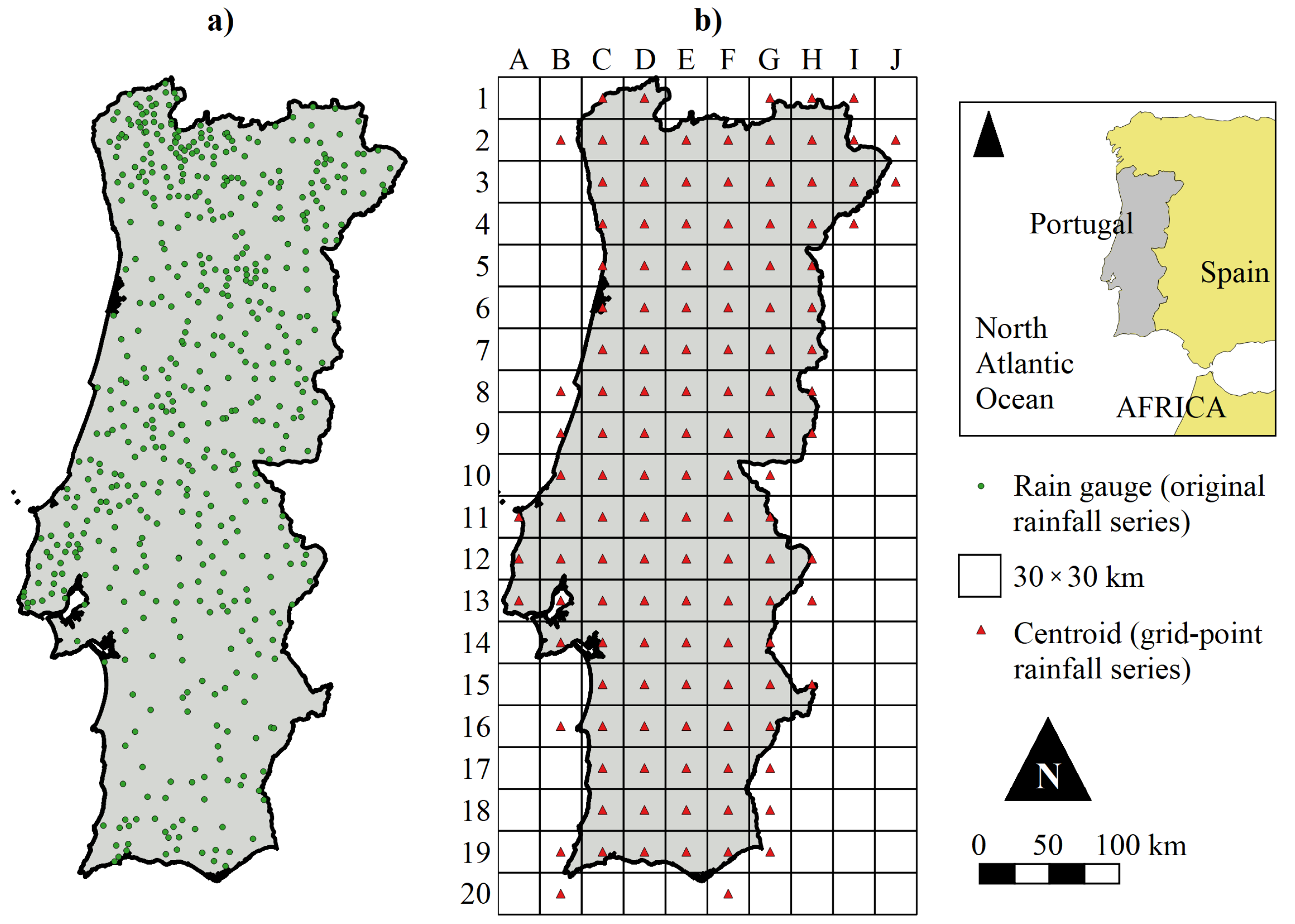
Long-term changes in rainfall have a strong effect on water security, surface runoff, soil water content, replenishment of groundwater supply, hydropower generation, agriculture production, and eventually the economic development of a territory [1]. Thus, the evaluation of rainfall trends is vital for inspecting the impact of climate change on water resources for its planning and management. In this case, the climate change denotes changes in the totality of attributes that define climate, and involves changes in sea surface and continental temperature, rainfall patterns, winds, ocean currents, and other measures of Earth’s climate that are clearly related to global warming [2]. Of particular concern is the possibility that global warming causes the hydrologic cycle to change, resulting, for instance, in fluctuations from intensification to deintensification, and vice versa, of important and previously well-defined water cycle variables, such as temperature and rainfall [3]. Whereas worldwide temperature displays a clear upward trend—e.g., Rahmstorf et al. [4]—no seasonally or annually consistent trend exists for global rainfall. Furthermore, it is acknowledged that global warming increases the risk of drought in several ways, making droughts more frequent, severe, and persistent. In accordance with the Intergovernmental Panel on the Climate Change (IPCC) Fourth Assessment Report [5] and all succeeding reports, the average temperature at the Earth’s surface rises, more evaporation occurs, which, in turn, increases overall precipitation. Therefore, a warming climate is expected to increase rainfall in many areas, but factors such as shifting wind patterns and changes in the ocean currents that drive the world’s climate system will also cause some areas to experience decreased rainfall as often pointed out for some regions of southern Europe. Herein, this work addresses (i) rainfall trends, which are assumed to be closely associated with atmospheric circulation patterns, i.e., (ii) links with teleconnection patterns, and (iii) areal extent or regionalised occurrences of drought. The study area is mainland Portugal (with an area of 89,015 km), located in the western part of the Iberian Peninsula, which is also the south westernmost part of Europe, facing the North Atlantic Ocean (Figure 1).
The statistical analysis of seasonal and annual rainfall data for Portugal is still relevant for climate modelling [6], particularly because such timescales may conceal highly different spatial rainfall regimes and trends. Portugal is characterised by a Mediterranean climate with warm and dry summers and mild cool and wet winters. The major natural factors that largely determine the Portuguese climate are the latitude, the sharp hilly terrain, ranging from 0–1993 m above sea level, and the weak ocean current that flows south along the coast of the country [7]. The within-the-year and year-to-year rainfall variability can change the fresh water budget (from excess to deficit) of any given season or year, mainly for the southern and north-eastern regions of Portugal where such variability is more pronounced. The unpredictability of the rainfall regime and the intermittent data acquisition by the rain gauge network, in some cases, lead to considerable repercussions on all the studies related to surface water availability and quality. Furthermore, the importance of rainfall changes in Portugal (e.g., periods of drier-than-normal conditions) linked to recurring and persistent, large-scale patterns of pressure and circulation anomalies have not been matched by sufficient scientific attention.
Most papers published in the last two decades dealing with rainfall trends over mainland Portugal are limited to certain areas or regions within the country with a sparse rain gauges’ network—but more notably, they have a relatively short time-series. For instance, the analyses by Costa and Soares [8] provide a qualitative classification of 106 daily rainfall series from stations located in southern Portugal and evaluate trends and other temporal rainfall patterns from 1955–1999. Santos and Fragoso [9] focus on the spatial and temporal variability of precipitation indices in northern Portugal from 1950–2000 using 39 meteorological stations, detecting negative or downward rainfall trends at winter (from October to March) and hydrological year (from October to September) timescales. The study by Da Silva et al. [10] is focused on trends in annual rainfall at a regional scale for a southern Portuguese catchment over 40 years from 1960–2000, finding significant rainfall reduction in the basin. Nunes and Lourenço [11] study the spatial variability and trends in monthly and annual rainfall based on rainfall series data from 42 stations during the period 1960–2011, relating the estimated trends to geographic variables to check for dependencies and spatial patterns in rainfall distribution. Santos et al. [12] analyse trends in selected rainfall indices on a seasonal basis from 1950–2003. The authors’ results revealed statistically significant negative trends in the months of March, April, and May mainly in northern and central Portugal, while weak positive or upward trends were detected from September through November. The rain gauges’ density and data series length limits the previous works on trends, in general. Despite this limitation, the authors recognise the heterogeneous and very complex spatial patterns of rainfall in Portugal. Contrastingly, Portela et al. [13,14] address long-term rainfall trends, their temporal variability and uncertainty over Portugal, using monthly, seasonal and annual rainfall series spanning from 1913–2019 at 532 rain gauges. Their findings support the hypothesis that the contrast between a less wet north, yet still wet, and an arid south is becoming much more marked. Although, the research of Portela et al. [13] represents the most comprehensive work on Portuguese rainfall trends to date (with a high number of stations covering a long time span), a connection to the large-scale atmospheric pressure see-saw in the North Atlantic region, i.e., the North Atlantic Oscillation (NAO) has been unconsidered.
The NAO is one of the most well-known teleconnection patterns [15] and generally refers to the basin-wide, meridional dipole pattern of sea-level pressure variability in the extratropical Atlantic. The NAO corresponds to the most important large-scale mode of atmospheric circulation in the winter season over the entire Northern Hemisphere. The connection between several climate variables, such as rainfall over Europe and the NAO, is widely recognised—e.g., Rousi et al. [16]. Rainfall in Portugal is somewhat shaped by many atmospheric circulation mechanisms, displaying a close relationship with the variability of the NAO. For instance, Santos et al. [17] established a solid connection between winter rainfall over Portugal (using three gridded monthly rainfall locations) and five weather regimes including the NAO; Trigo et al. [18] assessed the impact of NAO on winter rainfall and landslide events, but was limited to five sample areas in Lisbon District. These studies have pointed out the strong NAO influence upon the rainfall temporal variability in Portugal, mainly as regards to winter rainfall (from October–March), which dominates the rainfall regime of the country.
The above mentioned observations, and the uncertainty over the future NAO behaviour under a warming climate [16], motivated this study on climate variable trends, specifically of rainfall and the NAO teleconnection pattern. Within this framework, the present study aims at better understanding the climate system in Portugal during the century from 1919–2019 by (i) revisiting rainfall trends, at different timescales (e.g., quarterly, seasonal and annual) based on over a hundred grid-point rainfall data evenly distributed all over the country, and by (ii) establishing links between trends of these representative rainfall series and teleconnection patterns—i.e., climate variability links between non-contiguous geographic regions [19]. Via robust and commonly used techniques in detecting trends of variables in climatology and hydrology fields, the main objective of this research work is to examine fluctuations of trend and change detection of rainfall and North Atlantic Oscillation index (NAOI) time-series along with their likely relationship. Such a relationship or teleconnection is established under the assumption that fluctuations in the NAO have a strong effect on rainfall changes [20,21].
The paper is organised as follows: Section 2 describes the database and the methodology used in this study. The data used are (i) 126 grid-point rainfall series over a regular mesh, representing a subset of the aforementioned 532 rain gauges, and (ii) different NAOI series, both variables from 1919–2019. Section 3 demonstrates the results obtained, with particular emphasis on the teleconnection between the rainfall trends and NAOI trends from the extensively studied winter period from December through March. In Section 4, the main results are discussed, including an additional analysis of regionalised moderate and severe droughts for Portugal to elaborate on the achieved findings; the conclusions and perspectives of future work are presented in Section 5.
2. Material and Models
2.1. Grid-Point Rainfall and North Atlantic Oscillation Index Data Set
For addressing rainfall trends in Portugal and their teleconnection to a fluctuation of atmospheric pressure over the North Atlantic Ocean, this study combines (i) grid-point rainfall series with (ii) NAO indices (NAOI), i.e., NAO definitions based on the difference of normalised sea level pressure (SLP) between Lisbon, Portugal and Reykjavik, Iceland [22]. Point-scale rainfall data are gridded to create a regional dataset, which in turn, emulates different gridded products for climate monitoring—e.g., E-OBS for Europe [23], and APHRODITE for Asia [24]. Thus, grid-point rainfall series are constructed from previously published point-scale rainfall data carefully curated from 532 rain gauges in Portugal, Figure 1a [13]. One of the advantages of using gridded rainfall is that areal coverage of rainfall at a given location can be expeditiously estimated [25], which also simplifies the analysis of the envisaged spatial correlation between rainfall and climatic drivers. The analysed period covers 100 hydrological years, that is, from October 1919 to September 2019. The rainfall timescales considered are: the two quarters with higher input to annual rainfall in Portugal, namely, from (a) October–December (OND), and (b) January–March (JFM), representing almost 75% of the annual rainfall [14]; the period from (c) December–March (DJFM); and (d) the hydrological year (ANN) which, in Portugal, runs from October of a given year to September of the next one. The NAOI timescales coupled with the previous rainfall timescales are: nOND (October–December), nJFM (January–March), nDJFM (December–March), and nANN (October–September). The quarterly, DJFM and ANN rainfalls were aggregated from monthly values, where the NAOI realisations are directly retrieved from Hurrell and NCAR [22]. From the year 1919 to 2019, 126 complete grid-point rainfall series and one NAOI series per timescale, with 100 random values each, are implemented.
Figure 1.
Schematic location of (a) the 532 rain gauges, i.e., original rainfall series—from Portela et al. [13]—and (b) the constructed mesh with the 126 centroids used for the rainfall trend analysis and teleconnection. Centroids’ coordinate referencing system: WGSM84, UTM zone 29 N; for instance, in metres C1 (527908 and 4652269) and F20 (617908 and 4082269).

The grid-point rainfall series were based on the Inverse Distance to a Power gridding method with an exponent of two, IDW2 [26], applied to monthly data from the 532 rain gauges aforementioned. This popular interpolation method has been used in many environmental applications—, e.g., Stahl et al. [27], Tveito et al. [28]. The grid cell size of km (Figure 1b) was set based on the typical grid lengths implemented by the World Meteorological Organization (WMO) for numerical weather prediction (NWP) systems [29]. That being said, the Portuguese continuum was divided into a 200-cell grid, but selecting only those within the country, i.e., 126 cells. Centroids were assigned to each of the selected cells (red triangles in Figure 1b) representing the location of the grid-point rainfall series and the core of the analyses. This involved allocating monthly rainfalls to such centroids from the set of 532 rain gauges (green bullets in Figure 1a). For a given month of a given year, the rainfall at each grid point was the distance-weighted rainfall, with the IDW2 method, of the rainfalls in the same date at m surrounding rain gauges. Then, the 532 rain gauges were ranked by increasing distance to each grid point. The criteria to select m considered that the average weight for the set of 126 centroids of the mth closest rain gauges should not exceed approx. 0.5%. Such criteria resulted in closest rain gauges. This reconstruction process allowed completing 126 grid-point rainfall series of monthly data for the reference period from 1919–2019.
2.2. Monotonic and Sequential Trend Models
The main models utilised in this study for statistical analysis are mostly implemented in R (https://cran.r-project.org/; accessed on 10 December 2021). For each considered rainfall and NAOI timescale, the series constructed and retrieved, respectively, were assumed to have no autocorrelation. Given that each series is built upon 100 values, one value per hydrological year, randomness is ensured. Thus, the well-known rank-based nonparametric Mann–Kendall (MK) test [30] coupled with Sen’s slope estimator test [31] were applied to the grid-point rainfall series of the 126 centroids to determine rainfall variability and long-term monotonic trends at the timescales previously mentioned (OND, JFM, DJFM and ANN). A positive (negative) Sen’s slope estimate can be translated into a monotonic upward (downward) trend, which means that the variable consistently increases (decreases) through time.
The main model used for the teleconnection of rainfall changes and the NAO was the sequential Mann–Kendall (SQMK) test statistic [32]. This model allowed the estimation of the qualitative change and fluctuation over time in the trend of the NAOI series and of the grid-point rainfall series at the same timescales for trend estimation. In general, the SQMK test allows the detection of the approximate beginning of a developing trend on time-series . The SQMK test is computed using ranked values of the original values in analysis . The test statistic sets up a standardised series, a progressive-trend series, , which is expected to fluctuate around zero. The following steps were applied to calculate the series:
- The values of the original series were replaced by their ranks , arranged in ascending order.
- The magnitudes of , , were compared with , , and at each of the comparisons, the number of cases were counted and denoted by .
- A statistic was defined as follows:
- The mean and variance of the test statistic were computed as:
- The sequential values of the statistic u() were then calculated as:
Likewise, a retrograde-trend series, u’, can be calculated backward, but in this application, only the series were considered for rainfall-NAO teleconnection—by means of the Pearson correlation coefficient, r [33].
3. Results
3.1. Spatial Distribution of the Grid-Point Rainfall and Their Trends
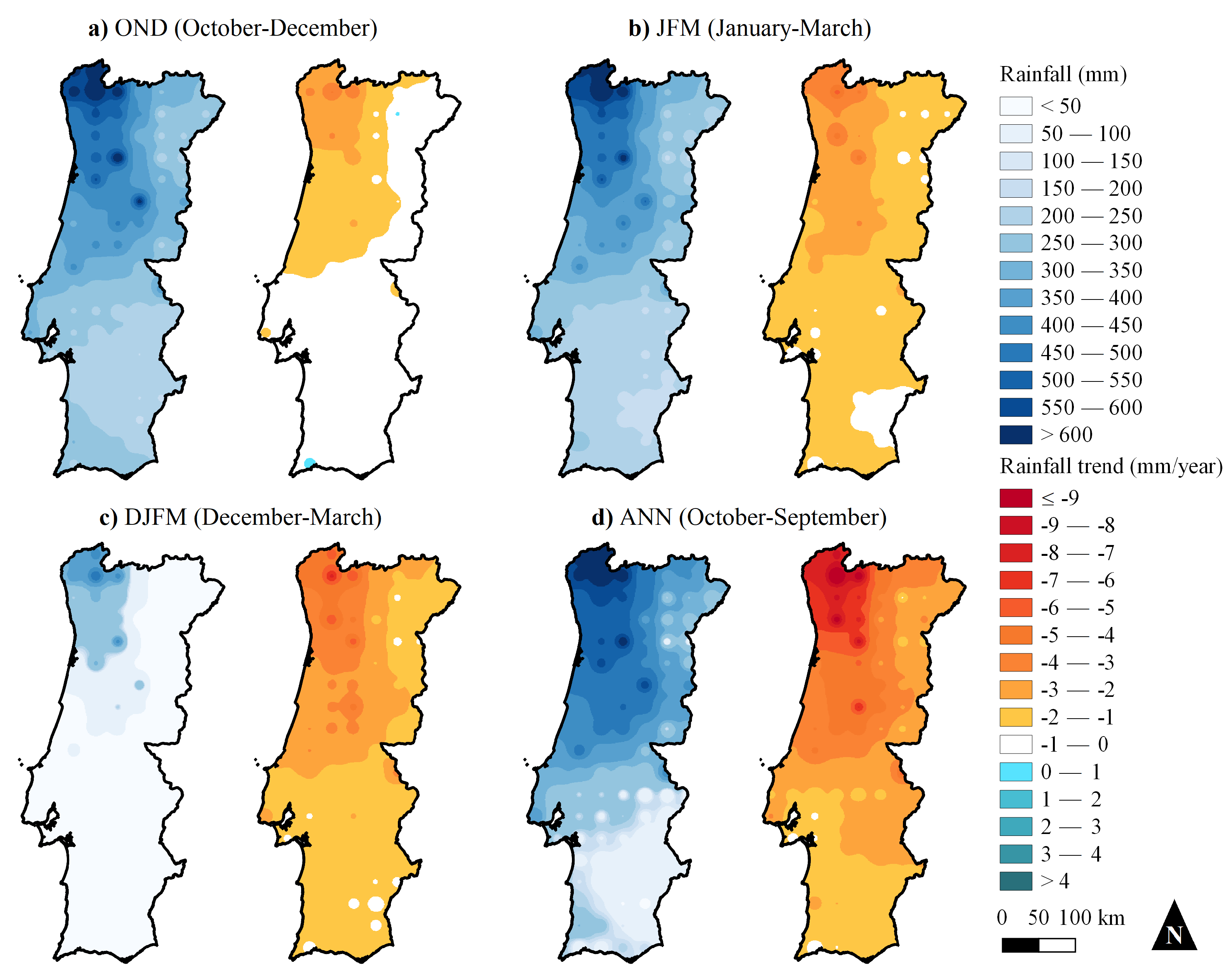
Before applying the MK and the Sen’s slope estimator tests, a characterisation of the quarterly, DJFM and annual, ANN, rainfall was done over Portugal based on the grid-point rainfall data (1919–2019) at the regular mesh with 126 centroids used in the study (left panel of each combo in Figure 2). This characterisation was performed to couple it with the estimated trends, and thus to have indicators for monitoring climate change based merely on rainfall. According to the rainfall distribution maps, there is considerable climatic variability from north to south, the north-western region being wetter than the dry southeast. The average gridded rainfall in Portugal during the 100-year period varies from 186 to 773 mm in OND, 156 to 834 mm in JFM, 223 to 1156 mm in DJFM and 447 to 2208 mm in the hydrological year, ANN. The spatially weighted rainfall averages are: 322 mm in OND, 310 mm in JFM, 432 mm in DJFM and 854 in ANN. The sum of the two considered quarters (OND and JFM) represent 74% of ANN.
Likewise, the estimates from the Sen’s slope estimator are also mapped (right side of each combo in Figure 2), regardless their statistical significance. The gridded rainfall trends range in mm per year from, to 0.2 in OND; to in JFM; to in DJFM; and to for ANN. The latter shows that the trends have a generalised downward behaviour more markedly in the north-west where the rainfall totals are much higher. Moreover, the rainfall characterisation and trend patterns of Figure 2 totally agree with those in Portela et al. [14], although such study makes use of point-scale data (532-point data) and considered a slightly longer time span, from 1913–2019, with a subperiod particularly wetter.
3.2. Sequential Observed Trends in Rainfall and in the North Atlantic Oscillation
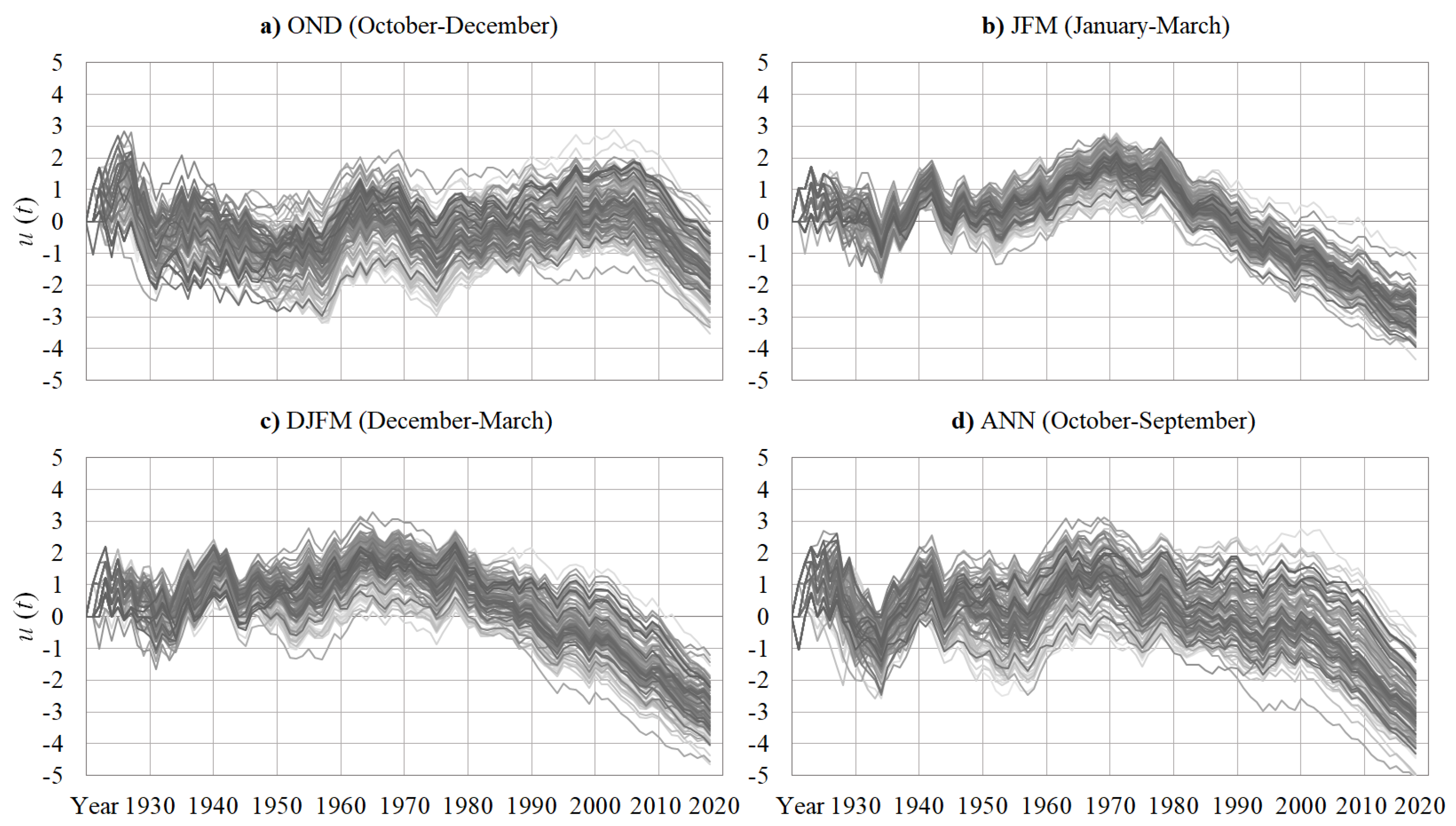
The previous rainfall trend values have been determined from a straight linear fit to the data, but the rainfall changes may have been irregular during the analysed 100-year period (1919–2019). For instance, a calculated trend could be due to a relatively abrupt step change, with the remainder of the series being fairly flat. Thus, the sequential Mann–Kendall (SQMK) test was applied to the grid-point rainfall series, but also to the NAOI series, to examine the sequential trend values and to determine the behaviour in detail of the trend lines, i.e., the mix of upward (positive) and downwards (negative) trends that may be present in analysed time-series. To see how the trends fluctuated at the quarterly, December–March, and annual timescales; the graphing of the SQMK results is presented in Figure 3, for rainfall, and in Figure 4, for NAOI.
As shown in Figure 2 (right side of each combo), all locations are experiencing rainfall downward trends regardless of the timescale (except for a tiny southern stripe in OND). However, by adding the SQMK graphs (Figure 3), it is found that the grid-point rainfall series actually denote discontinuous periods of upward and downward trends—based on the positive and negative values of , respectively. For the 126 centroids, Figure 3 shows harmonious trend lines with differences within their development depending on the considered timescale. The trends for the 126 OND rainfall series (Figure 3a), are negative from 1919 through 1960 followed by 50 years of generalised upward trends and ending with an abrupt change to negative values from 2010 onwards. For the second quarter, JFM (Figure 3b), the trends denote a positive behaviour from the start of the beginning of the reference period until the late 1960s, and rapidly changed to sustained negative values for the remaining years. The same behaviour of the trends is present in the 4-month timescale, DJFM (Figure 3c). Regarding the ANN series (Figure 3d), the trends seem to have a fuzzy performance with positive and negative values alternating from 1919 until the early 1970s; up from this point, the trends show a gradually downward behaviour, although it is much more steep from the year 2010 on. Based on these, the importance is placed at the period from 1960–1970, as most of the rainfall trends appear to start having more variability around that time, as evidenced by other studies—e.g., Baines and Folland [34].
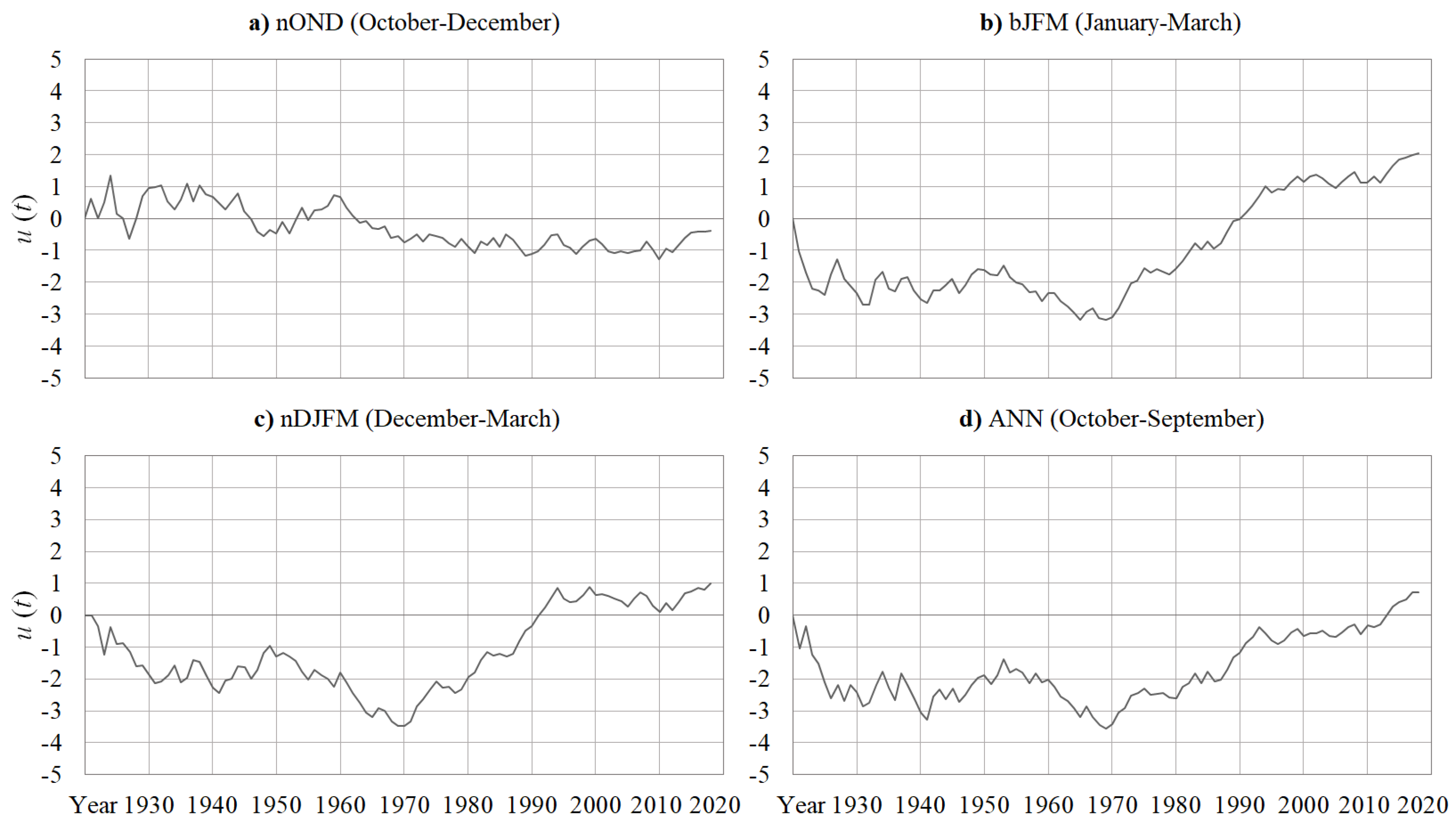
Additionally, regarding the progressive of the NAOI series, the most important changes of the trends occur during the same identified period for the rainfall series (ca. around 1960 and 1970). For instance, the trends in nOND (Figure 4a) are weak and intermittent during the first few years. Nevertheless, from the 1960 on, the nOND trends are negative, relatively stronger and sustained. In contrast, the nJFM series denotes negative values with a flat response from the year 1919 until 1968 (Figure 4b). Up from 1968 onwards, the shows rapidly increasing positive values. A remarkable feature of the nDJFM NAOI is its trend towards a more positive phase over the past 50 years (Figure 4c). The same feature is present in the nANN NAOI trends (Figure 4d) with a steady upward direction from the early 1970s on. In addition, visual inspection of Figure 3 and Figure 4 suggests a similar position of breaking points or changes of trends in the behaviour in the rainfall and NAO. This illustrates that when analysing trends in a dataset, not only should the MK value and Sen’s slope be considered, but also their sequential MK values for a better understanding of the trends’ development.
3.3. Teleconnection between the Grid-Point Rainfall Trends and the NAOI Trends
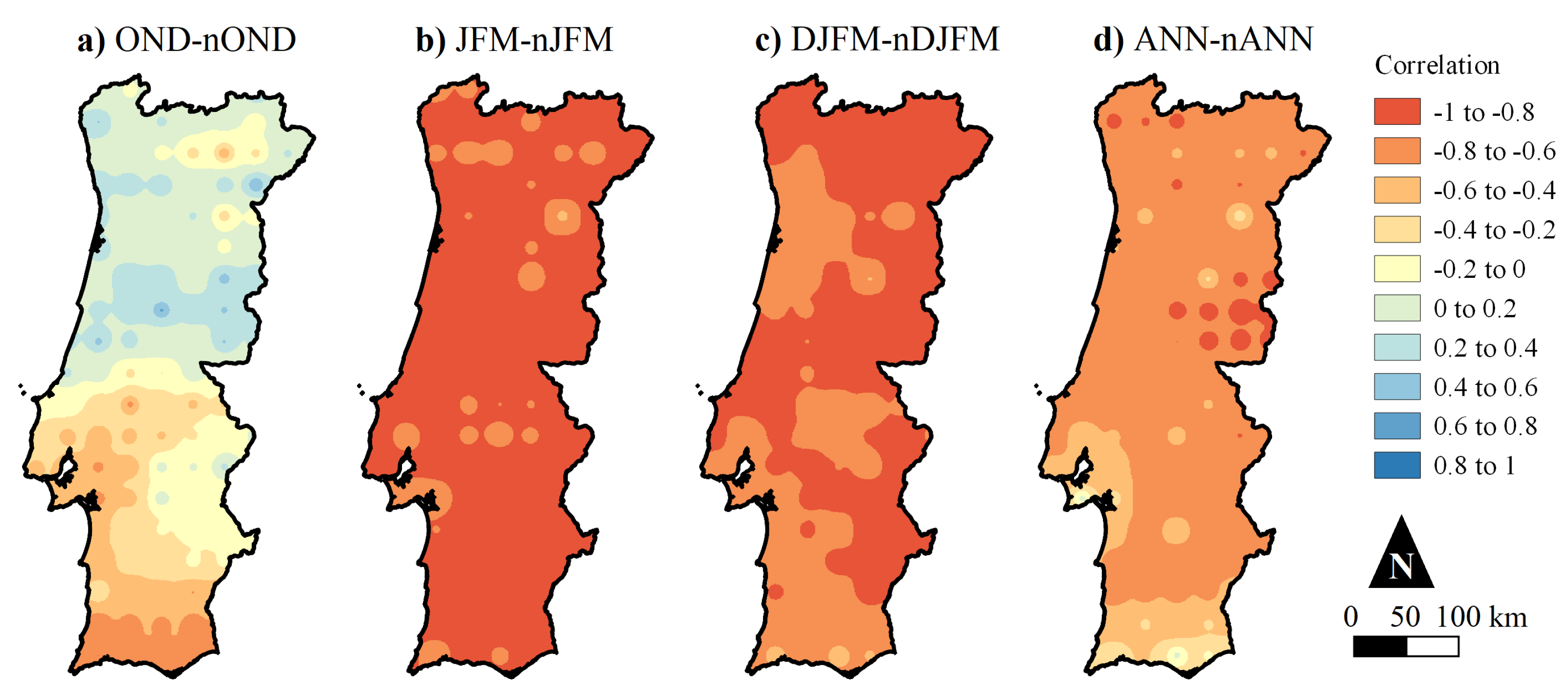
As mentioned in Section 1, this paper focuses on the influences of the North Atlantic Oscillation (NAO, the large-scale atmospheric pressure see-saw in the North Atlantic region) on rainfall in mainland Portugal at different standard meteorological timescales. Besides the annual timescale, the focus is the wintertime (e.g., the period from December to March of next year) as it has been recognised that the influence of the oceanic and atmospheric patterns is more significant during the boreal winter [35]. Overall, the results in the previous subsection show that (i) the rainfall distribution in Portugal is spatially uneven, with more quantities in the north and less in the south, but with harmonic trends despite the estimated rainfall differences, and that (ii) the progressive-trend graphs of the two variables considered (grided rainfall and NAOI) tend to move in opposite directions, at least visually checking. Thus, the Pearson correlation coefficient, r, was applied to describe a pattern or relationship for teleconnection between the trends of the coupled values of the rainfall and NAOI at a same timescale, notwithstanding their statistical significance. The correlations, r, between the progressive-trend series of Figure 3 and Figure 4, respectively, are mapped in Figure 5. Note that, from the Fisher Z-Transformation [36] for a 100 sample size and significance level , r is significant when r .
According to Figure 5a, rainfall-NAO correlations for the first quarter (OND-nOND) range from to , denoting a contrasting distribution with more positive correlations in the north neutralising the negative ones in the southern coast (average correlation of ). Regarding the second quarter (JFM-nJFM), correlations are stronger, ranging from to , and on average of (Figure 5b). Note that the trends in JFM are more marked compared to those in OND (as shown on right panes of Figure 2). This clearly indicates a coherent relationship between rainfall changes in Portugal and the NAO signal. Such a pattern is still negatively strong over the country for the period from December through March (DJFM-nDJFM in Figure 5c), with correlation values ranging from to ( on average). Regarding the hydrological year (ANN-nANN in Figure 5d), the negative sign of correlation (from to ; on average) shows a very similar dipole-type pattern of the NAO influence on rainfall changes. These results reveal that this influence has a much larger extent during wintertime and that the atmospheric circulations over the North Atlantic can be considered as a major driver for rainfall across Portugal in JFM, DJFM and, to a lesser extent, in ANN.
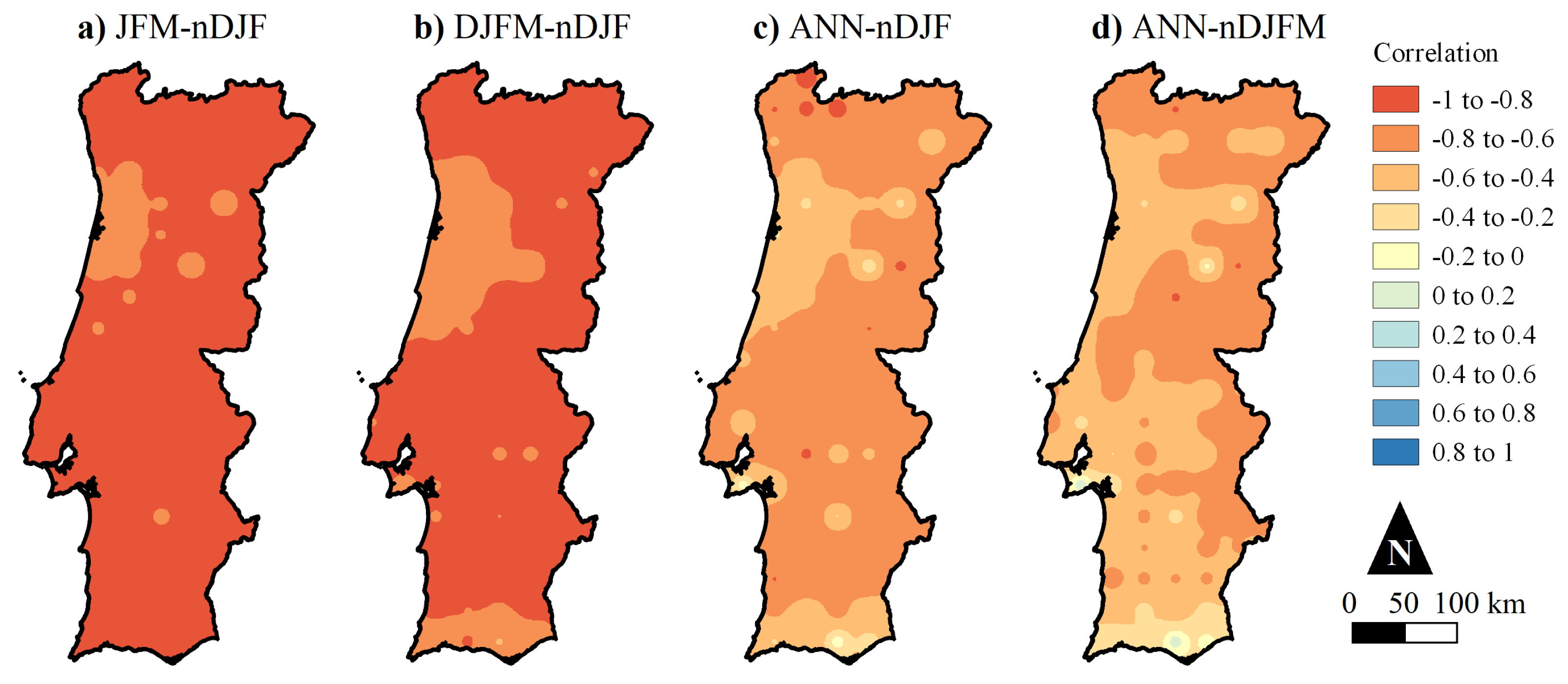
The establishment of the aforementioned relationships (Figure 5), motivated the feasibility of developing seasonal and annual prediction of rainfall trends based on preceding seasons of the NAO. The addition of preceding NAO seasons may provide information for the better understanding of rainfall variability and for skilful seasonal prediction. Actually, owing to a strong seasonal cycle of the stability at the base of the oceanic mixed layer, any irregularity in SLP can persist below the mixed-layer and influence rainfall in the following seasons [37]. Analogously, the delayed influence or persistence, in some cases, of the NAO indices trends on rainfall trends of the coming or longer seasons, is assessed. Thus, (i) two winter NAOI series, namely, the already used nDJFM, and the one resulting from the inclusion of the quarterly index from December–February (nDJF); coupled with (ii) three rainfall timescales (JFM, DJFM, and ANN) are considered, as shown in Figure 6.
According to Figure 6a, the nDJF has a solid footprint on the following one-month lagged rainfall season, i.e., JFM with a correlation on average of , ranging from to . Figure 6b shows that nDJF has a persistent effect on the four-month rainfall timescale DJFM with on average (ranging from to ). Compared to the previous two rainfall timescales, the highly influenced area by nDJF decreases, but being still significant, on annual rainfall (Figure 6c) with a correlation on average of (ranging from to ). Similarly, nDJFM NAOI has an apparent controlling influence on annual rainfall (average correlation of ), but with weaker values (in comparison to the nDFJ results) along the coast and in a tiny strip in southern Portugal with positive correlation (), as shown in Figure 6d. In summary, the proposed bivariate teleconnections appear to act as a bridge to link the North Atlantic Ocean variability to the seasonal (particularly in winter) and annual rainfall in Portugal.
4. Discussion
In this paper, grid-point rainfall trends in Portugal during the 1919–2019 century are studied, as depicted in Figure 2. In general, the results are in agreement with the identified annual rainfall decrease, since the late 1960s, of up to 9.0 mm per year in some parts of southern Europe [38]. Different from recent research, where the influence of oceanic patterns are widely studied, such as El Niño Southern Oscillation (ENSO) [39,40,41], this research study focuses on the effect of the North Atlantic Oscillation (NAO). A teleconnection of mathematical definitions of NAO for observed regional rainfall changes in Portugal is proposed in this study. The bivariate teleconnection revealed the intrinsic correlations between trends of both NAO and rainfall at different timescales. To illustrate the possible influences of NAO trends on the rainfall, correlation maps were produced (Figure 5 and Figure 6). From the graphical correlation representation, it can be observed that the NAO climate patterns (e.g., seasonal and annual NAOI) have some negative, or inverse, correlation with rainfall trends all over Portugal, although they are negatively stronger in the short winter NAOI series (e.g., nDJF and nJFM).
4.1. Persistent Influence of the North Atlantic Oscillation on Rainfall Trends
Figure 6 displays the correlation between rainfall anomalies and the NAO. The strength of the correlation exhibits a marked spatiotemporal variability. The winter three-month (JFM), four-month (DJFM) and annual (ANN) rainfall trends in Portugal appear to be highly related to the NAO on average, meaning that sustained and more below-normal rainfall (translated into downward trends) may be expected, with a sustained increase of positive winter NAO (with upward trends). The latter could imply that a persistent positive (negative) phase of NAO in winter favours longer dry (wet) spells over the country. This could involve the slight bimodal rainfall distribution in Portugal with a first peak in early November and another one in late December. Moreover, rainfall from late April until mid-September contributes the least to annual rainfall as aforementioned, and thus, it has been kept out from this analysis. The rainfall anomalies in such a dry period are significantly less related to NAO (not shown), as expected, meaning that they can be subject to other large-scale pressure patterns—, such as the East Atlantic (EA) and Scandinavian (SCAND) patterns [42]—, in contrast to the wet period. This supports the idea that a short three-month winter NAO index (e.g., nDJF) is enough to give some hints of the lagged rainfall trends in Portugal.
In addition, rainfall-NAO lagged correlations or correlations on the following rainfall seasons (e.g., ANN-nDJF in Figure 6c), although with lower values, present an analogous structure of the simultaneous teleconnection results (e.g., ANN-nANN in Figure 5d). This is also in agreement with similar teleconnection studies. For instance, Luppichini et al. [43] investigate the link between NAO and rainfall trends (in a Mediterranean area) calculated by the Spearman’s correlation coefficient, claiming that the bivariate correlation is negative in winter and weakly positive during summer. Regarding mainland Portugal, as the study area in this work, de Lima et al. [44] analyse the relationships from 1941–2007 between the variability of the NAOI and several rainfall indices related to 57 stations, concluding that the decreasing trends observed in the rainfall indices appear to be related to the prevalence of the positive phase of the NAO. The latter patterns, obtained with point-scale rainfall data, are in consonance with the results here obtained. This evidences the opposing response of rainfall over Portugal to the NAO. Such opposing response is in agreement with Brandimarte et al. [45], suggesting that when the NAO index is well above normal (upward trend), the patterns for rainfall are more localised, with an increased chance of lower rainfall (downward trend) in Mediterranean Europe. Finally, the relationship between rainfall trends and NAO trends is consistent whether gridded or point-scale rainfall data are used, despite the inherent differences.
4.2. Regionalised Droughts in Portugal during 1919–2019
Taking advantage of the grid-point rainfall series (Figure 1b) and their trends (Figure 2 and Figure 3), an exploratory analysis on droughts was performed to detect how consistent the spatiotemporal rainfall trends are with droughts, assuming that decreasing rainfall trends determine more occurrences of drought [46]. Drought, as a natural phenomenon, is intrinsically part of Earth’s climate and occurs in all climatic zones with neither warning nor recognition of administrative borders or of political and economic differences. Drought can be perceived as sustained and regionally broad occurrences of below average natural water availability [47].
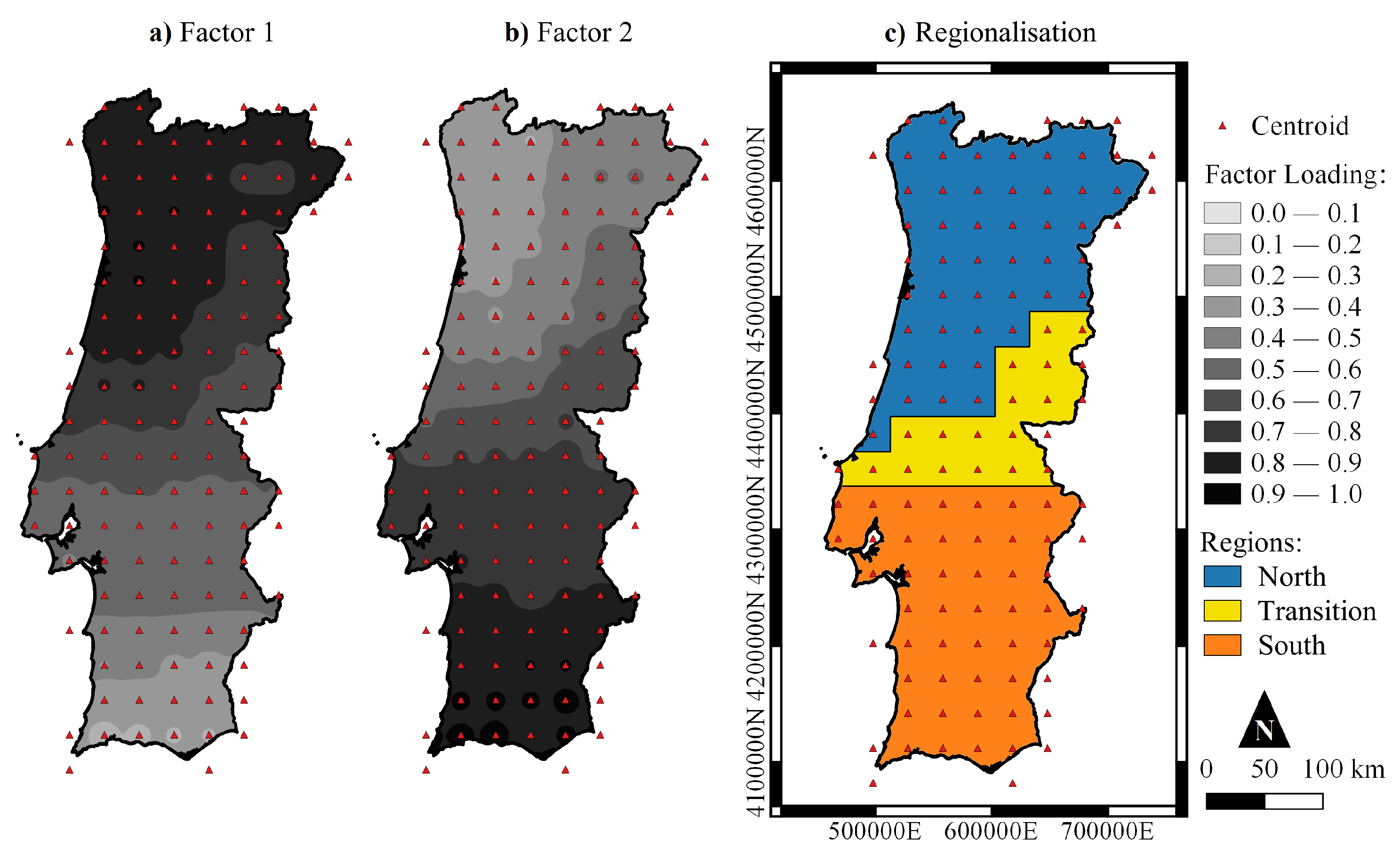
Prior to the drought analysis and having in mind the extensive spatial coverage of such a creeping phenomenon, empirical orthogonal functions were applied to the gridded rainfall to regionalise climatic conditions changes in Portugal. Empirical orthogonal functions, such as the principal component analysis (PCA) and principal factor analysis (PFA) have been widely applied in climate-related studies [48]. These techniques (known as the eigenvector analysis) were used to reduce the spatial and temporal gridded rainfall data to manageable, physically interpretable abstractions by expressing the variance of such sampled data field in a reduced number of the original 126 centroid dimensions. The eigenvector analysis, specifically factor analysis (FA), including both PCA and PFA, was applied to the 100-year annual grid-point rainfall data from 1919–2019 at the 126 centroids, i.e., to the matrix X. Additionally, when analysing droughts based on spatiotemportal data only, it is necessary to identify regions or centroids, in this case, with similar temporal patterns and put them together in space [49]. Thus, a two-step process was applied based on the FA (i) to group the centroids, and then (ii) to spatially average the gridded rainfall series of the centroids in the identified homogeneous region. The first two unrotated principal components suggested non-random signals when the scree test [50] was applied to the eigenvalue series (not shown here). The number of principal components was two, explaining 91.9% of the total variance of the original problem. This helped to obtain the factor loadings, in this application, with two factors retained (Factor 1, F1 and Factor 2, F2; explaining 47.1% and 44.8% of total variance, respectively), using Varimax raw for factor rotation, and PCA as an extraction method [51]—the retention of more factors was also tested but is meaningless in this application due to a probable overfactoring.
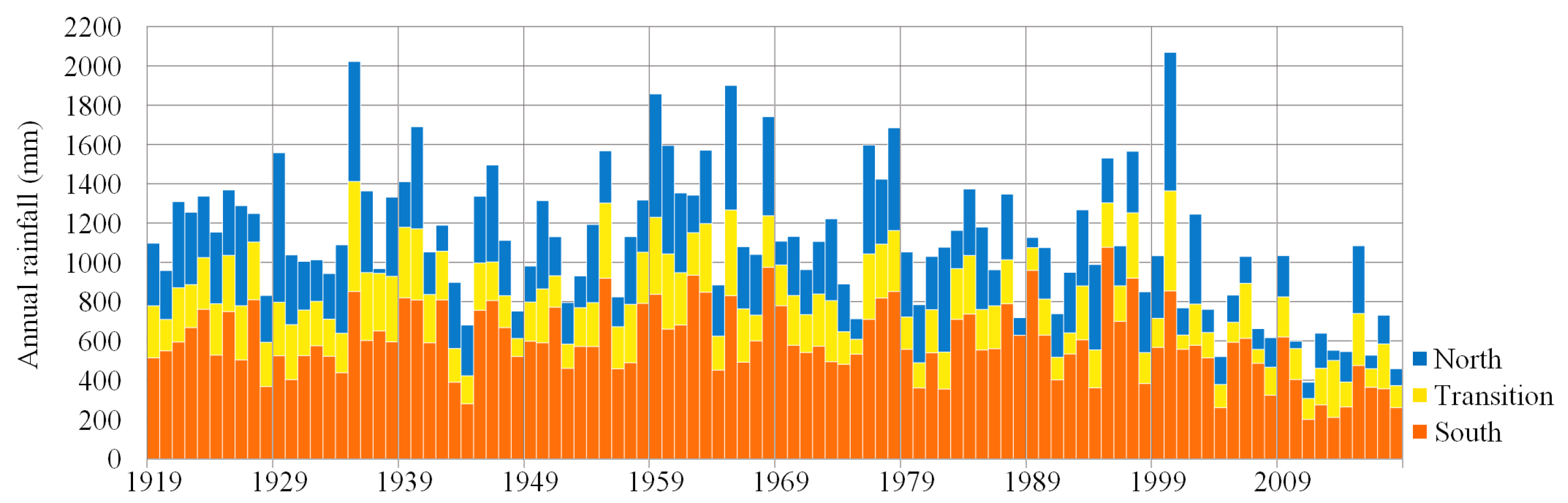
The mapping of factor loadings was conducted to classify the climatological patterns [52]. The homogeneous regions were delimited based on the rotated factor loadings of centroids with correlations higher than (Figure 7a,b). The overlap of the factor loading mapping enabled the annual gridded rainfall field to be divided into coherent homogeneous regions (Figure 7c). This clearly discriminates mainland Portugal into distinctive climatic regions: north (with 54 centroids only related to F1), transition (including 20 centroids with factor loadings higher than in both factors), and south (considering 52 centroids solely linked to F2). By performing the factor analysis, a mature climatic regionalisation has been established in terms of annual gridded rainfall encompassing all the 126 centroids. This clustering of centroids was followed by the spatial average of the grid-point rainfall series, at different timescales (e.g., monthly and annual), for each of the three identified homogeneous regions. By way of example of the regionalised grid-point rainfall series, Figure 8 presents the annual rainfall values from 1919–2019 in the north, transition and south. Accordingly, the southern homogeneous region is the driest region with an average over the 100-year studied period of 591.1 mm. The equivalent value for the north is 1119.7 mm (the wettest region) whereas for the transition homogeneous region, it is 822.9 mm—note that for the same century, the weighted annual rainfall average is 854.0 mm, as previously mentioned.
To detect the drought in Portugal during the century studied, the standardised precipitation index (SPI), developed by McKee et al. [53], was used. The SPI, as it is defined, was applied only to the regionalised monthly gridded rainfalls (north, transition, and south—Figure 7c) to assess two different drought types and timescales, namely: (i) moderate and severe droughts for (ii) 6-month and 12-month SPI, i.e., SPI6 and SPI12, with a smoothing factor, M, of 5 and 6, respectively [54]. The drought categories adopted were those of Agnew [55]. Shorter durations of SPI were not considered, since they are usually linked to water deficits and to the short-term change drought characteristics [56]. As the timescale increases, the response of SPI6 and SPI12 to short-term rainfall decelerates, resulting in more stable and well-defined droughts. Both the SPI6 and SPI12 better reflect long-term changes in the drought of river runoff, groundwater level and reservoir water storage capacity, for instance.
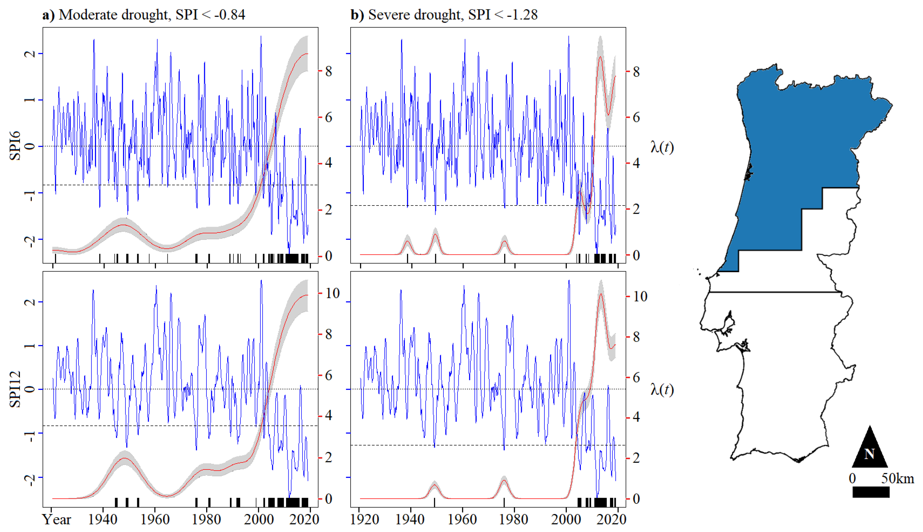
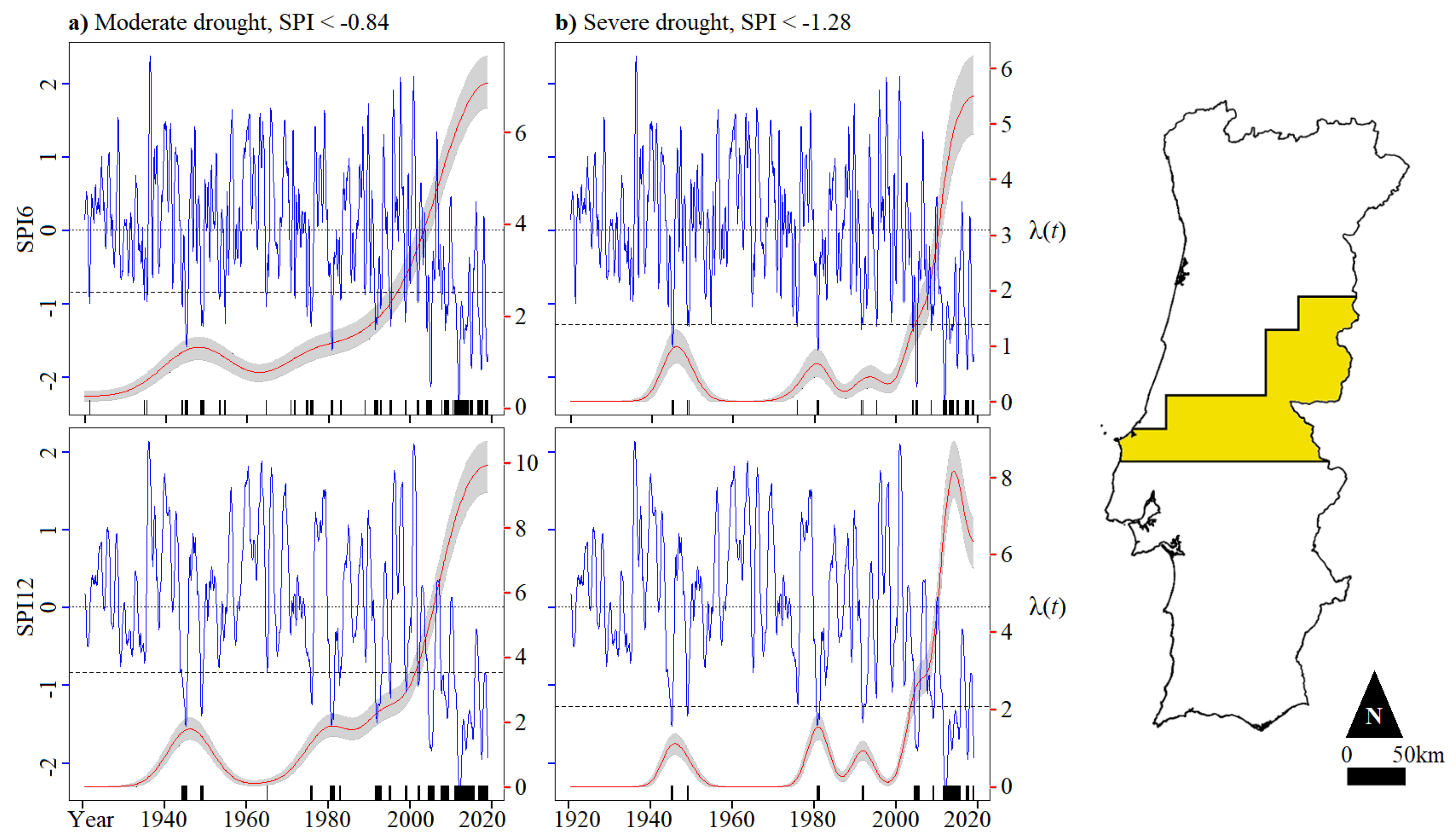
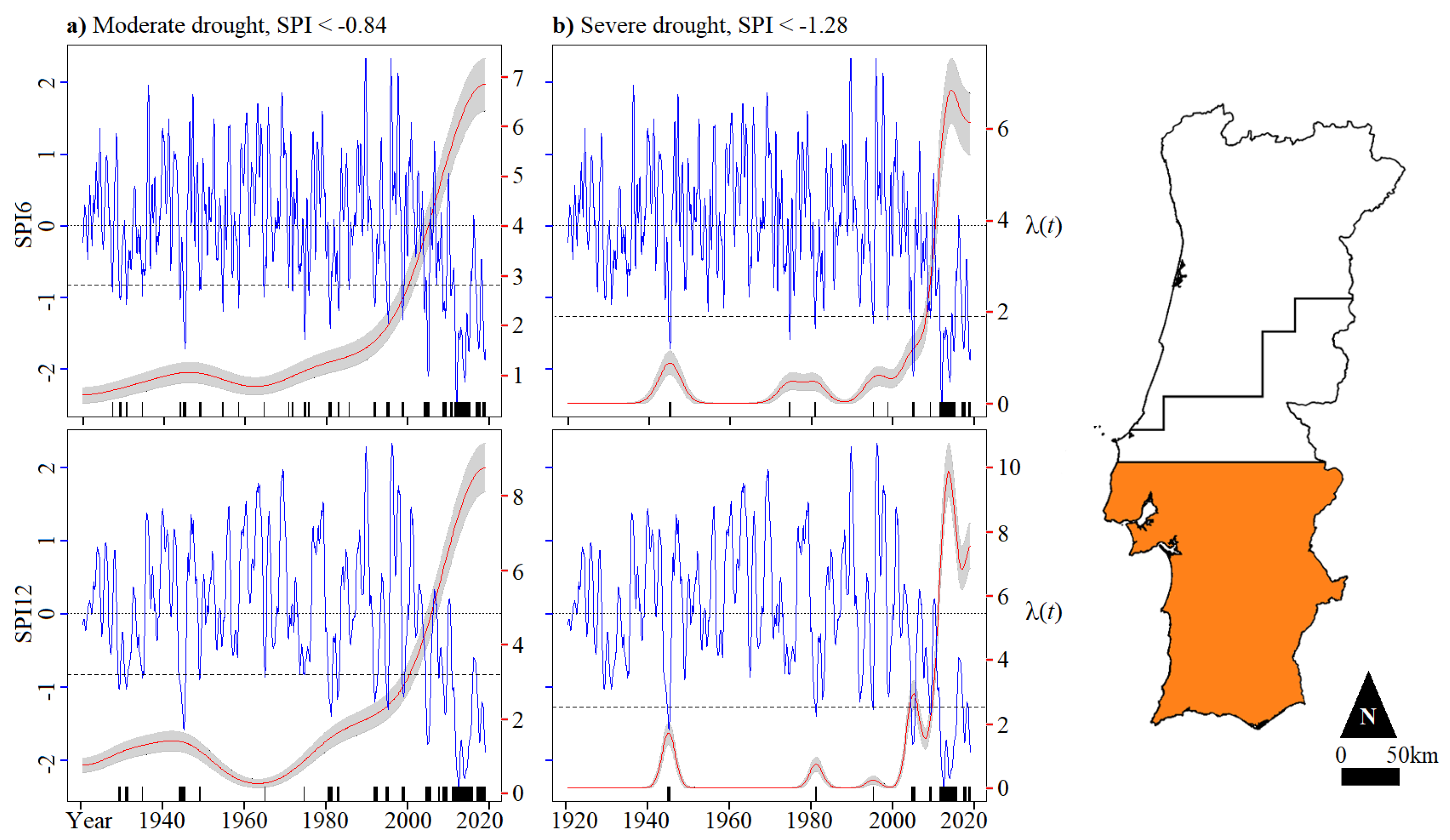
The analysis of the changes in the frequency of occurrence of the periods under drought conditions was addressed by applying a kernel occurrence rate estimator (KORE), according to the stepwise approach applied by Silva et al. [57], Silva [58], including the generation of pseudodata outside of the observation interval, by the straightforward method of reflection for an amplitude of three times the bandwidth. The KORE was applied to the times of occurrence of the periods under drought conditions from 1919–2019, i.e., to the temporal positions of SPI6 (1191 monthly positions) and SPI12 (1184 monthly positions) lower than the drought thresholds and , for moderate and severe droughts [55], respectively; and thus, to calculate the annual frequency of the periods under drought conditions, , for the northern, transitional and southern climatic regions (Figure 9, Figure 10 and Figure 11).
The confidence bands around , related to the uncertainties from the frequency analysis, were constructed based on bootstrap resampling [59,60], as described in Silva et al. [57]. The red line in Figure 9, Figure 10 and Figure 11 shows that the frequency of periods under drought conditions is somewhat similar among the three homogeneous regions, with more occurrences in recent years exhibiting significant inter-annual variability. In general, there is an increase for moderate droughts (Figure 9a, Figure 10a, and Figure 11a), for any SPI timescale, with from 2 to 10 periods under drought conditions per year, from 2000 onward. Almost the same behaviour is reflected for the severe droughts (Figure 9b, Figure 10b, and Figure 11b), but with a more rapid and prominent frequency increase around the years 2010–2011. Both drought types should have been driven by rainfall deficits.
From the regionalised rainfall series in Figure 8, it can be said that the 100 analysed hydrological years have experienced extensive rainfall deficiencies in Portugal. For instance, in the most recent 50 years, i.e., from 1969–2019, the number of years with below-average rainfall conditions in the homogeneous climatic regions are: 35 in the north, 33 in the transition, and 32 in the south, which in turn, represent more than 60% of the total occurrences for the 100-year period (1919–2019). In addition, this dry 50-year period has contributed to a long-term statistical decline in rainfall trends as shown by the negative rainfall trends of Figure 3. The failure of the wet season, in terms of downward trends or sustained below-average rainfall conditions, apparently has contributed to more intense and frequent drought occurrences in recent years. Despite the correlation between standardised precipitation indices (or drought trends) and teleconnection indices, not fully explored here, a comparison of the time dependent drought occurrence rates and of the progressive trend series of the NAOI (Figure 4) gives some insights about the NAO being a leading mode of climate variability influencing some of the drought events in Portugal. By visual inspection of Figure 4, Figure 9a, Figure 10a, and Figure 11a; the apparent increase of moderate droughts in the last 50 years seem to be linked to the upward trends in the nJFM, nDJFM, and nANN NAOI series, which in turn, is a period with dominance of positive NAOI. While the decline of severe drought—particularly for SPI12 (Figure 9b, Figure 10b, and Figure 11b)—after the year 2013 has suggested a return to less severe patterns for Portugal, the progressive seasonal and annual trends of both rainfall (DJFM and ANN in Figure 3) and NAO during and since this year suggest otherwise. Thus, severe drought frequency may increase again accompanied by a stronger influence of recently more positive and unusual winter season and annual NAO indices [61].
5. Conclusions and Future Work
This paper describes the long-term grid-point rainfall trends in the context of climate change, recent regionalised rainfall decline and drought events for mainland Portugal teleconnected, in most cases, to the trends of mathematical descriptions of the North Atlantic Oscillation during the century from 1919–2019. In summary, this study highlights the usefulness of the constructed grid-point rainfall data (Figure 1b), which has allowed for clearly detecting different atmospheric links’ patterns in the Portuguese continuum. While natural rainfall variability in Portugal is large, and intrinsically influenced by the NAO, based on the current research it seems likely that drying, or downward rainfall trends, across northwest and the most southern Portugal cannot be explained by changes in the NAO alone—see Figure 6. Therefore, the analysis of shifts in other atmospheric circulation patterns may improve the teleconnection analysis such as the East Atlantic (EA) pattern and the East Atlantic/West Russia pattern (EA/WR) [62,63].
Furthermore, the gridded rainfall series has also allowed the identification of climatic regions of Portugal in terms of rainfall. Based on the rainfall series of the three identified homogeneous or climatic regions (Figure 7 and Figure 8), the past two decades have observed the return of widespread rainfall deficits across the country, particularly in southern Portugal—which may be part of the recognised hot spot at the Iberian Peninsula southwest regions of the pattern “dry gets drier”, i.e., the DD paradigm [64]. The same behaviour is reflected in terms of increased moderate and severe droughts in the same decades (Figure 9, Figure 10 and Figure 11). In addition, given that rainfall influences the streamflow dynamics of many Portuguese regions [65], the more sudden and intensified rainfall decreases from the late 1960s may be accompanied by much larger reductions in streamflow, particularly in the north and south. This decrease emerges against a background of significant upward trends of the NAO—an irregular fluctuation of atmospheric pressure over the North Atlantic Ocean, with a strong effect on the rainfall regime over Portugal particularly during the wet or winter season. This unusual dominance of positive phases of the NAO has persisted for decades.
Finally, according to one of the latest issues by the IPCC [66], climate change is already affecting every inhabited regions across the globe, with human influence to many observed changes in climate extremes, rainfall and drought events. Thus, advances in the knowledge of climate processes (as the contribution of this research work for mainland Portugal) may, in turn, improve the estimates of the response of the surface Essential Climate Variables (ECV)—e.g., surface water vapour, pressure, temperature and rainfall [67]—to increasing radiative forcing in the potential future warming [68].
Author Contributions
Conceptualization, L.A.E.; methodology, L.A.E.; software, L.A.E.; validation, L.A.E.; formal analysis, L.A.E.; investigation, L.A.E.; resources, L.A.E.; data curation, L.A.E. and M.M.P.; writing—original draft preparation, L.A.E.; writing—review and editing, M.M.P.; visualization, L.A.E.; supervision, M.M.P.; project administration, L.A.E.; funding acquisition, M.M.P. All authors have read and agreed to the published version of the manuscript.
Funding
This research was supported by the Foundation for Science and Technology’s support through funding UIDB/04625/2020 from the research unit CERIS, and by the European Union’s Horizon 2020 research and innovation programme under grant agreement No 101003534.
Institutional Review Board Statement
Not applicable.
Informed Consent Statement
Not applicable.
Data Availability Statement
The data that support the findings of this study are available on request from the corresponding author.
Acknowledgments
The authors are grateful for the Foundation for Science and Technology’s support through funding UIDB/04625/2020 from the research unit CERIS. In addition, this project has received funding from the European Union’s Horizon 2020 research and innovation programme under grant agreement No 101003534.
Conflicts of Interest
The authors declare no conflict of interest.
References
- Zeleňáková, M.; Purcz, P.; Blišt’an, P.; Alkhalaf, I.; Hlavatá, H.; Portela, M.M.; Silva, A.T. Precipitation trends detection as a tool for integrated water resources management in Slovakia. Management 2017, 13, 17. [Google Scholar] [CrossRef]
- Harvey, L.D. Global Warming; Taylor & Francis Group: Abingdon, UK, 1999. [Google Scholar]
- Koutsoyiannis, D. Revisiting the global hydrological cycle: Is it intensifying? Hydrol. Earth Syst. Sci. 2020, 24, 3899–3932. [Google Scholar] [CrossRef]
- Rahmstorf, S.; Foster, G.; Cahill, N. Global temperature evolution: Recent trends and some pitfalls. Environ. Res. Lett. 2017, 12, 054001. [Google Scholar] [CrossRef]
- Change, C. IPCC fourth assessment report. Phys. Sci. Basis 2007, 2, 580–595. [Google Scholar]
- Pereira, S.C.; Carvalho, D.; Rocha, A. Temperature and Precipitation Extremes over the Iberian Peninsula under Climate Change Scenarios: A Review. Climate 2021, 9, 139. [Google Scholar] [CrossRef]
- Abrantes, F.; Rodrigues, T.; Rufino, M.; Salgueiro, E.; Oliveira, D.; Gomes, S.; Oliveira, P.; Costa, A.; Mil-Homens, M.; Drago, T. The climate of the Common Era off the Iberian Peninsula. Clim. Past 2017, 13, 1901–1918. [Google Scholar] [CrossRef] [Green Version]
- Costa, A.C.; Soares, A. Trends in extreme precipitation indices derived from a daily rainfall database for the South of Portugal. Int. J. Climatol. A J. R. Meteorol. Soc. 2009, 29, 1956–1975. [Google Scholar] [CrossRef]
- Santos, M.; Fragoso, M. Precipitation variability in Northern Portugal: Data homogeneity assessment and trends in extreme precipitation indices. Atmos. Res. 2013, 131, 34–45. [Google Scholar] [CrossRef]
- Da Silva, R.M.; Santos, C.A.; Moreira, M.; Corte-Real, J.; Silva, V.C.; Medeiros, I.C. Rainfall and river flow trends using Mann–Kendall and Sen’s slope estimator statistical tests in the Cobres River basin. Nat. Hazards 2015, 77, 1205–1221. [Google Scholar] [CrossRef]
- Nunes, A.; Lourenço, L. Precipitation variability in Portugal from 1960 to 2011. J. Geogr. Sci. 2015, 25, 784–800. [Google Scholar] [CrossRef]
- Santos, M.; Fonseca, A.; Fragoso, M.; Santos, J.A. Recent and future changes of precipitation extremes in mainland Portugal. Theor. Appl. Climatol. 2019, 137, 1305–1319. [Google Scholar] [CrossRef]
- Portela, M.M.; Espinosa, L.A.; Zelenakova, M. Long-term rainfall trends and their variability in mainland Portugal in the last 106 years. Climate 2020, 8, 146. [Google Scholar] [CrossRef]
- Portela, M.M.; Espinosa, L.A.; Zelenakova, M. Updated Rainfall Series and Their Trends for Mainland Portugal (1913–2019). WIT Trans. Ecol. Environ. 2021, 250, 3–12. [Google Scholar]
- Hurrell, J.W. Influence of variations in extratropical wintertime teleconnections on Northern Hemisphere temperature. Geophys. Res. Lett. 1996, 23, 665–668. [Google Scholar] [CrossRef]
- Rousi, E.; Rust, H.W.; Ulbrich, U.; Anagnostopoulou, C. Implications of winter NAO flavors on present and future European climate. Climate 2020, 8, 13. [Google Scholar] [CrossRef] [Green Version]
- Santos, J.; Corte-Real, J.; Leite, S. Weather regimes and their connection to the winter rainfall in Portugal. Int. J. Climatol. A J. R. Meteorol. Soc. 2005, 25, 33–50. [Google Scholar] [CrossRef]
- Trigo, R.M.; Zêzere, J.L.; Rodrigues, M.L.; Trigo, I.F. The influence of the North Atlantic Oscillation on rainfall triggering of landslides near Lisbon. Nat. Hazards 2005, 36, 331–354. [Google Scholar] [CrossRef]
- North, G.R.; Pyle, J.A.; Zhang, F. General Circulation of the Atmosphere | Teleconnections. Encyclopedia of Atmospheric Sciences; Elsevier: Amsterdam, The Netherlands, 2014; Volume 1. [Google Scholar]
- Espinosa, L.A.; Portela, M.M. Rainfall trends over a small island teleconnected to the North Atlantic oscillation-the case of Madeira Island, Portugal. Water Resour. Manag. 2020, 34, 4449–4467. [Google Scholar] [CrossRef]
- Espinosa, L.A.; Portela, M.M.; Rodrigues, R. Rainfall trends over a North Atlantic small island in the period 1937/1938–2016/2017 and an early climate teleconnection. Theor. Appl. Climatol. 2021, 144, 469–491. [Google Scholar] [CrossRef]
- Hurrell, J.; Ncar, S. The Climate Data Guide: Hurrell North Atlantic Oscillation (NAO) Index (Station-Based). 2020. Available online: https://climatedataguide.ucar.edu/climate-data/hurrell-north-atlantic-oscillation-nao-index-station-based (accessed on 10 December 2021).
- Hofstra, N.; Haylock, M.; New, M.; Jones, P.; Frei, C. Comparison of six methods for the interpolation of daily, European climate data. J. Geophys. Res. Atmos. 2008, 113, 3–9. [Google Scholar] [CrossRef] [Green Version]
- Yatagai, A.; Kamiguchi, K.; Arakawa, O.; Hamada, A.; Yasutomi, N.; Kitoh, A. APHRODITE: Constructing a long-term daily gridded precipitation dataset for Asia based on a dense network of rain gauges. Bull. Am. Meteorol. Soc. 2012, 93, 1401–1415. [Google Scholar] [CrossRef]
- Prasanna, V.; Subere, J.; Das, D.K.; Govindarajan, S.; Yasunari, T. Development of daily gridded rainfall dataset over the Ganga, Brahmaputra and Meghna river basins. Meteorol. Appl. 2014, 21, 278–293. [Google Scholar] [CrossRef]
- Bartier, P.M.; Keller, C.P. Multivariate interpolation to incorporate thematic surface data using inverse distance weighting (IDW). Comput. Geosci. 1996, 22, 795–799. [Google Scholar] [CrossRef]
- Stahl, K.; Moore, R.; Floyer, J.; Asplin, M.; McKendry, I. Comparison of approaches for spatial interpolation of daily air temperature in a large region with complex topography and highly variable station density. Agric. For. Meteorol. 2006, 139, 224–236. [Google Scholar] [CrossRef]
- Tveito, O.; Wegehenkel, M.; van der Wel, F.; Dobesch, H. Spatialisation of climatological and meteorological information with the support of GIS (Working Group 2). In The Use of Geographic Information Systems in Climatology and Meteorology, Final Report; COST (European Cooperation in Science and Technology): Amsterdam, The Netherlands, 2006; pp. 37–172. [Google Scholar]
- WMO. Guidelines on Ensemble Prediction Systems and Forecasting; World Meteorological Organisation: Geneva, Switzerland, 2012. [Google Scholar]
- Kendall, M.G. Rank Correlation Methods, 4th ed.; Griffin: London, UK, 1948. [Google Scholar]
- Sen, P.K. Estimates of the regression coefficient based on Kendall’s tau. J. Am. Stat. Assoc. 1968, 63, 1379–1389. [Google Scholar] [CrossRef]
- Sneyres, R. Technical Note No. 143 on the Statistical Analysis of Time Series of Observation; World Meteorological Organisation: Geneva, Switzerland, 1990. [Google Scholar]
- Pearson, K. Notes on the history of correlation. Biometrika 1920, 13, 25–45. [Google Scholar] [CrossRef]
- Baines, P.G.; Folland, C.K. Evidence for a rapid global climate shift across the late 1960s. J. Clim. 2007, 20, 2721–2744. [Google Scholar] [CrossRef] [Green Version]
- Kosaka, Y.; Xie, S.P. Recent global-warming hiatus tied to equatorial Pacific surface cooling. Nature 2013, 501, 403–407. [Google Scholar] [CrossRef] [Green Version]
- Yevjevich, V.M. Probability and Statistics in Hydrology; Water Resources Publication: Fort Collins, CO, USA, 1972; pp. 237–241. [Google Scholar]
- Choi, Y.W.; Ahn, J.B.; Kryjov, V.N. November seesaw in northern extratropical sea level pressure and its linkage to the preceding wintertime Arctic Oscillation. Int. J. Climatol. 2016, 36, 1375–1386. [Google Scholar] [CrossRef]
- Knmi, I. Trends in annual and summer precipitation across Europe between 1960 and 2015. Royal Netherlands Meteorological Institute (KNMI). 2017. Available online: http://www.knmi.nl (accessed on 7 June 2022).
- Chen, X.; Wang, S.; Hu, Z.; Zhou, Q.; Hu, Q. Spatiotemporal characteristics of seasonal precipitation and their relationships with ENSO in Central Asia during 1901–2013. J. Geogr. Sci. 2018, 28, 1341–1368. [Google Scholar] [CrossRef] [Green Version]
- Li, X.; Zhang, K.; Gu, P.; Feng, H.; Yin, Y.; Chen, W.; Cheng, B. Changes in precipitation extremes in the Yangtze River Basin during 1960–2019 and the association with global warming, ENSO, and local effects. Sci. Total Environ. 2021, 760, 144244. [Google Scholar] [CrossRef] [PubMed]
- Emmanuel, I. Linkages between El Niño-Southern Oscillation (ENSO) and precipitation in West Africa regions. Arab. J. Geosci. 2022, 15, 1–11. [Google Scholar] [CrossRef]
- Sánchez-López, G.; Hernández, A.; Pla-Rabès, S.; Trigo, R.M.; Toro, M.; Granados, I.; Sáez, A.; Masqué, P.; Pueyo, J.J.; Rubio-Inglés, M.; et al. Climate reconstruction for the last two millennia in central Iberia: The role of East Atlantic (EA), North Atlantic Oscillation (NAO) and their interplay over the Iberian Peninsula. Quat. Sci. Rev. 2016, 149, 135–150. [Google Scholar] [CrossRef] [Green Version]
- Luppichini, M.; Barsanti, M.; Giannecchini, R.; Bini, M. Statistical relationships between large-scale circulation patterns and local-scale effects: NAO and rainfall regime in a key area of the Mediterranean basin. Atmos. Res. 2021, 248, 105270. [Google Scholar] [CrossRef]
- De Lima, M.I.P.; Santo, F.E.; Ramos, A.M.; Trigo, R.M. Trends and correlations in annual extreme precipitation indices for mainland Portugal, 1941–2007. Theor. Appl. Climatol. 2015, 119, 55–75. [Google Scholar] [CrossRef]
- Brandimarte, L.; Di Baldassarre, G.; Bruni, G.; D’Odorico, P.; Montanari, A. Relation between the North-Atlantic Oscillation and hydroclimatic conditions in Mediterranean areas. Water Resour. Manag. 2011, 25, 1269–1279. [Google Scholar] [CrossRef]
- Bevacqua, E.; Zappa, G.; Lehner, F.; Zscheischler, J. Precipitation trends determine future occurrences of compound hot–dry events. Nat. Clim. Chang. 2022, 12, 350–355. [Google Scholar] [CrossRef]
- Tallaksen, L.M.; Van Lanen, H.A. Hydrological Drought: Processes and Estimation Methods for Streamflow and Groundwater; Elsevier: Amsterdam, The Netherlands, 2004. [Google Scholar]
- White, D.; Richman, M.; Yarnal, B. Climate regionalization and rotation of principal components. Int. J. Climatol. 1991, 11, 1–25. [Google Scholar] [CrossRef]
- Lyra, G.B.; Oliveira-Júnior, J.F.; Zeri, M. Cluster analysis applied to the spatial and temporal variability of monthly rainfall in Alagoas state, Northeast of Brazil. Int. J. Climatol. 2014, 34, 3546–3558. [Google Scholar] [CrossRef]
- Cattell, R.B. The scree test for the number of factors. Multivar. Behav. Res. 1966, 1, 245–276. [Google Scholar] [CrossRef]
- Yarnal, B. Synoptic Climatology in Environmental Analysis: A Primer; CRC Press: Boca Raton, FL, USA, 1993. [Google Scholar]
- Jennrich, R.I. Rotation methods, algorithms, and standard errors. In Factor Analysis at 100; Routledge: London, UK, 2007; pp. 329–350. [Google Scholar]
- McKee, T.B.; Doesken, N.J.; Kleist, J. The relationship of drought frequency and duration to time scales. In Proceedings of the 8th Conference on Applied Climatology, Anaheim, CA, USA, 17–22 January 1993; Volume 17, pp. 179–183. [Google Scholar]
- Espinosa, L.A.; Portela, M.M.; Pontes Filho, J.D.; Studart, T.M.D.C.; Santos, J.F.; Rodrigues, R. Jointly modeling drought characteristics with smoothed regionalized SPI series for a small island. Water 2019, 11, 2489. [Google Scholar] [CrossRef] [Green Version]
- Agnew, C. Using the SPI to Identify Drought. In Drought Network News (1994–2001); University College London: London, UK, 2000; Available online: https://digitalcommons.unl.edu/droughtnetnews/ (accessed on 10 December 2021).
- Liu, D.; You, J.; Xie, Q.; Huang, Y.; Tong, H. Spatial and temporal characteristics of drought and flood in Quanzhou based on standardized precipitation index (SPI) in recent 55 years. J. Geosci. Environ. Prot. 2018, 6, 25–37. [Google Scholar] [CrossRef] [Green Version]
- Silva, A.T.; Portela, M.; Naghettini, M. Nonstationarities in the occurrence rates of flood events in Portuguese watersheds. Hydrol. Earth Syst. Sci. 2012, 16, 241–254. [Google Scholar] [CrossRef] [Green Version]
- Silva, A. Nonstationarity and Uncertainty of Extreme Hydrological Events. Ph.D. Dissertation, IST/UTL, Lisbon, Portugal, 2017. [Google Scholar]
- Cowling, A.; Hall, P.; Phillips, M.J. Bootstrap confidence regions for the intensity of a Poisson point process. J. Am. Stat. Assoc. 1996, 91, 1516–1524. [Google Scholar] [CrossRef]
- Mudelsee, M. The bootstrap in climate risk analysis. In In Extremis; Springer: Berlin/Heidelberg, Germany, 2011; pp. 44–58. [Google Scholar]
- Eade, R.; Stephenson, D.; Scaife, A.; Smith, D. Quantifying the rarity of extreme multi-decadal trends: How unusual was the late twentieth century trend in the North Atlantic Oscillation? Clim. Dyn. 2022, 58, 1555–1568. [Google Scholar] [CrossRef]
- Barnston, A.G.; Livezey, R.E. Classification, seasonality and persistence of low-frequency atmospheric circulation patterns. Mon. Weather Rev. 1987, 115, 1083–1126. [Google Scholar] [CrossRef]
- Tošić, I.; Putniković, S. Influence of the East Atlantic/West Russia pattern on precipitation over Serbia. Theor. Appl. Climatol. 2021, 146, 997–1006. [Google Scholar] [CrossRef]
- Greve, P.; Orlowsky, B.; Mueller, B.; Sheffield, J.; Reichstein, M.; Seneviratne, S.I. Global assessment of trends in wetting and drying over land. Nat. Geosci. 2014, 7, 716–721. [Google Scholar] [CrossRef]
- Nunes, A.N.; Lopes, P. Streamflow Response to Climate Variability and Land-Cover Changes in the River Beça Watershed, Northern Portugal. In River Basin Management; IntechOpen: London, UK, 2016; pp. 61–80. [Google Scholar]
- Allan, R.P.; Hawkins, E.; Bellouin, N.; Collins, B. Summary for Policymakers; IPCC: Geneva, Switzerland, 2021. [Google Scholar]
- Bojinski, S.; Verstraete, M.; Peterson, T.C.; Richter, C.; Simmons, A.; Zemp, M. The concept of Essential Climate Variables in support of climate research, applications, and policy. Bull. Am. Meteorol. Soc. 2014, 95, 1431–1443. [Google Scholar] [CrossRef]
- Hébert, R.; Lovejoy, S.; Tremblay, B. An observation-based scaling model for climate sensitivity estimates and global projections to 2100. Clim. Dyn. 2021, 56, 1105–1129. [Google Scholar] [CrossRef]
Figure 2.
Average rainfall and Sen’s slope estimates (right and left side of each combo, respectively) for Portugal, based on the grid-point rainfall, for the 100 hydrological year period from 1919–2019 (IDW2 interpolation method used for mapping).
Figure 2.
Average rainfall and Sen’s slope estimates (right and left side of each combo, respectively) for Portugal, based on the grid-point rainfall, for the 100 hydrological year period from 1919–2019 (IDW2 interpolation method used for mapping).

Figure 3.
Progressive-trend series u(t in grey scales, unitless, of the quarterly OND, JFM; four-monthly DJFM, and annual ANN grid-point rainfall series for Portugal (based on the 126 centroids of Figure 1b).
Figure 3.
Progressive-trend series u(t in grey scales, unitless, of the quarterly OND, JFM; four-monthly DJFM, and annual ANN grid-point rainfall series for Portugal (based on the 126 centroids of Figure 1b).

Figure 4.
Progressive-trend series u(t, unitless, of the quarterly nOND, nJFM; four-monthly nDJFM, and annual nANN NAO indices, NAOI; station-based indices based on the difference of SLP between Lisbon, Portugal and Reykjavik, Iceland—based on the data from Hurrell and NCAR [22].
Figure 4.
Progressive-trend series u(t, unitless, of the quarterly nOND, nJFM; four-monthly nDJFM, and annual nANN NAO indices, NAOI; station-based indices based on the difference of SLP between Lisbon, Portugal and Reykjavik, Iceland—based on the data from Hurrell and NCAR [22].

Figure 5.
Teleconnection between the grid-point rainfall trends and NAOI trends from 1919–2019. Spatial distribution of the Pearson correlation coefficient, r, between the progressive-trend series, u(t, of OND, JFM, DJFM and ANN rainfall; and nOND, nJFM, nDJFM and nANN NAOI, respectively (IDW2 interpolation method used for mapping).

Figure 6.
Teleconnection between the grid-point rainfall trends and NAOI trends from 1919–2019. Spatial distribution of the Pearson correlation coefficient, r, between the progressive-trend series, u(t), of JFM-nDJF, DJFM-nDJF, ANN-nDJF, and ANN-nDJFM (IDW2 interpolation method used for mapping).
Figure 6.
Teleconnection between the grid-point rainfall trends and NAOI trends from 1919–2019. Spatial distribution of the Pearson correlation coefficient, r, between the progressive-trend series, u(t), of JFM-nDJF, DJFM-nDJF, ANN-nDJF, and ANN-nDJFM (IDW2 interpolation method used for mapping).

Figure 7.
Factor loadings (correlation between observed variables and latent common factors) for the annual 126 gridded rainfall series (1919–2019) in (a) Factor 1 and (b) Factor 2. (c) Regionalisation of three identified climatic regions based on factor analysis, namely, north, transition, and south—coordinates WGS84 (UTM zone 29N), IDW2 interpolation method used for mapping the factor loadings.

Figure 8.
Annual rainfall from 1919–2019 at each of the climatic regions averaged out of the total 126 grid-point rainfall series clustered from the factor analysis, i.e., at the north (54 centroids), transition (20 centroids) and south (52 centroids).
Figure 8.
Annual rainfall from 1919–2019 at each of the climatic regions averaged out of the total 126 grid-point rainfall series clustered from the factor analysis, i.e., at the north (54 centroids), transition (20 centroids) and south (52 centroids).

Figure 9.
Northern region. Time dependent occurrence rates, λ(t) (year−1), in red, and confidence band in grey of (a) moderate and (b) severe droughts for SPI6 and SPI12 in blue. The horizontal-dashed lines different to zero represent the drought thresholds and vertical ticks, with SPI below them.
Figure 9.
Northern region. Time dependent occurrence rates, λ(t) (year−1), in red, and confidence band in grey of (a) moderate and (b) severe droughts for SPI6 and SPI12 in blue. The horizontal-dashed lines different to zero represent the drought thresholds and vertical ticks, with SPI below them.

Figure 10.
Transitional region. Time dependent occurrence rates, λ(t) (year−1), in red, and confidence band in grey of (a) moderate and (b) severe droughts for SPI6 and SPI12 in blue. The horizontal-dashed lines different to zero represent the drought thresholds and vertical ticks, with SPI below them.

Figure 11.
Southern region. Time dependent occurrence rates, λ(t) (year−1), in red, and confidence band in grey of (a) moderate and (b) severe droughts for SPI6 and SPI12 in blue. The horizontal-dashed lines different to zero represent the drought thresholds and vertical ticks, with SPI below them.
Figure 11.
Southern region. Time dependent occurrence rates, λ(t) (year−1), in red, and confidence band in grey of (a) moderate and (b) severe droughts for SPI6 and SPI12 in blue. The horizontal-dashed lines different to zero represent the drought thresholds and vertical ticks, with SPI below them.

Publisher’s Note: MDPI stays neutral with regard to jurisdictional claims in published maps and institutional affiliations. |
© 2022 by the authors. Licensee MDPI, Basel, Switzerland. This article is an open access article distributed under the terms and conditions of the Creative Commons Attribution (CC BY) license (https://creativecommons.org/licenses/by/4.0/).
Share and Cite
MDPI and ACS Style
Espinosa, L.A.; Portela, M.M. Grid-Point Rainfall Trends, Teleconnection Patterns, and Regionalised Droughts in Portugal (1919–2019). Water 2022, 14, 1863. https://doi.org/10.3390/w14121863
AMA Style
Espinosa LA, Portela MM. Grid-Point Rainfall Trends, Teleconnection Patterns, and Regionalised Droughts in Portugal (1919–2019). Water. 2022; 14(12):1863. https://doi.org/10.3390/w14121863
Chicago/Turabian StyleEspinosa, Luis Angel, and Maria Manuela Portela. 2022. "Grid-Point Rainfall Trends, Teleconnection Patterns, and Regionalised Droughts in Portugal (1919–2019)" Water 14, no. 12: 1863. https://doi.org/10.3390/w14121863
Note that from the first issue of 2016, this journal uses article numbers instead of page numbers. See further details here.