
Machine Learning and Multiple Imputation Approach to Predict Chlorophyll-a Concentration in the Coastal Zone of Korea


1
Department of Digital Convergence, Chonnam National University, Yeosu 59626, Korea
2
Department of Ocean Integrated Science, Chonnam National University, Yeosu 59626, Korea
3
Fishery Resource Management Research Institute Based on ICT, Chonnam National University, Yeosu 59626, Korea
4
Department of Multimedia, Chonnam National University, Yeosu 59626, Korea
*
Authors to whom correspondence should be addressed.
Water 2022, 14(12), 1862; https://doi.org/10.3390/w14121862
Submission received: 20 April 2022
/
Revised: 4 June 2022
/
Accepted: 7 June 2022
/
Published: 10 June 2022
(This article belongs to the Section Oceans and Coastal Zones)
Abstract
:The concentration of chlorophyll-a (Chl-a) is an integrative bio-indicator of aquatic ecosystems and a direct indicator that evaluates the ecological status of water bodies. In this study, we focused on predicting the Chl-a concentration in seawater using machine learning (after replacing missing values). To replace the missing values among marine environment observation data, a comparison experiment was performed using multiple built-in imputation methods (i.e., pmm, cart, rf, norm, norm.nob, norm.boot, and norm.predict) of the mice package in R. The cart method was selected as the most suitable. We generated each regression model using six machine learning algorithms (regression tree, support vector regression (SVR), bagging, random forest, gradient boosting machine (GBM), and extreme gradient boosting (XGBoost)) to predict the Chl-a concentration based on the complete imputed dataset. The prediction performance of the models was evaluated by four evaluation criteria using 10-fold cross-validation tests. XGBoost, an ensemble learning approach, outperformed other models in predicting the Chl-a concentration; SVR, a single model, also showed a good performance. The most important environmental factor in predicting the Chl-a concentration was an organic carbon particulate; however, dissolved oxygen also showed potential. This study was conducted with field observations in the spring and summer in the coastal zone of Korea. There exists a limit in machine learning applications, which excludes temporal and spatial factors. However, extensions to time series forecasting for deep learning or machine learning can lead to meaningful regional and seasonal analysis. It can also improve prediction performance as a result of the long-term data accumulation of field observations of more varied features (such as meteorological and hydrodynamic) besides water quality.
1. Introduction
Machine learning is fundamental to the meaningful processing of data that cannot be comprehended by the human brain. A machine-learning-based model learns from examples, provided in the form of inputs called features and outputs called labels, rather than being programmed with rules [1]. The adoption of data-intensive machine learning methods can be seen in all fields of science, technology, and commerce, such as in healthcare, manufacturing, education, financial modeling, policing, and marketing, resulting in more evidence-based decision making [2]. The value of data, also known as the oil of the 21st century, is rising in all industries, and the quantity and quality of data are essential issues for machine learning. A lack of data quality can take the form of missing, incomplete, inconsistent, inaccurate, redundant, and outdated data [3]. Most of the data observed in reality include missing information, mostly as a result of unexpected circumstances (e.g., equipment failure, power outages, bad weather, and communication failure); in some instances, more than half of the information may be missing [4]. Most statistical analyses can only be conducted on complete datasets. In other words, cases with missing values in at least one of the specified variables will be excluded from an analysis [5,6]. This leads to a reduced sample size, compromises statistical power, and can affect the accuracy of parameter estimates [5,7]. Missing values must be addressed before analyzing data, as ignoring or omitting them can lead to a biased and ineffective analysis [8]. Missing data can lead to a substantial amount of bias, make data processing and analysis more difficult, and reduce efficiency [9]. Training a machine learning model with such data affects the model quality and leads to incorrect interpretations and results. However, it is time-consuming and costly to discard existing data and repeat the observations.
The concentration of chlorophyll-a (Chl-a) is an integrative bio-indicator of aquatic ecosystems, representing marine phytoplankton biomass and primary productivity, and is a direct indicator for evaluating the ecological status of water bodies [10,11]. This includes features such as algal blooms, which degrade the water quality of marine and freshwater environments. Algal blooms commonly occur in receiving water bodies, causing potential water quality deterioration and often resulting in the depletion of oxygen, reduced water transparency, and decreased biodiversity in marine and freshwater environments [11,12]. Machine learning has been used instead of multiple regression to predict Chl-a concentration and algal blooms because of the complexity and non-linearity of environmental factors. However, most studies have focused on freshwater environments and not on marine environments. Some previous studies have attempted to implement various machine learning techniques to predict Chl-a concentrations, with the majority focused on freshwater systems and only a few on marine regions [10,11,13,14,15,16,17].
When a significant amount of data is missing, it is difficult to ensure the validity, accuracy, and representation of analysis results with a normal listwise deletion [9,18]. Therefore, instead of a listwise deletion (a common approach for missing data), we apply an imputation method that minimizes information loss by identifying the pattern of missing information based on raw data and replacing the missing values in the marine environment. Various missing imputation methods exist, such as simple univariate imputation, k nearest neighbors (KNN) imputation, and multiple imputation (MI). Among these, MI is superior to single imputation, which replaces missing values with a mean, median, mode, etc. [19,20,21,22,23]. MI is a multivariate imputation approach, which uses other features to predict the missing value of the current feature, is free from normal distribution assumptions, and can be applied to non-continuous variables [24,25,26]. This approach may be generally referred to as fully conditional specification (FCS) or multivariate imputation by chained equations (MICE) [27,28,29].
Some studies have predicted target variables through machine learning after imputation. In the medical field, there was a case in which the IgA nephritis binary classification problem was predicted after applying the method with the best performance among the various missing imputation methods [30]. In a freshwater environment, there have been cases of algal bloom predictions after imputation using the KNN method [31] and Chl-a concentration predictions after a comparison of six missing data imputation methods [32]. However, many imputation and machine learning technologies are not fully utilized in the fishery and marine fields.
Therefore, our study utilized techniques such as multiple imputation and machine learning on marine coastal ecosystem observation data. We attempted to predict the Chl-a concentration and derived the importance of input features for the target variable (Chl-a concentration) in the marine field.
A Google Scholar search containing all three keywords (imputation, chlorophyll-a, and machine learning) showed approximately 150 cases over the last two years (as of the beginning May 2022). There were approximately 359,000 machine learning cases, 19,000 chlorophyll-a cases, and 25,000 imputation cases in the single-keyword search. The small number of convergence studies containing the three keywords demonstrates the need for this study.
2. Materials and Methods
2.1. Study Area and Data
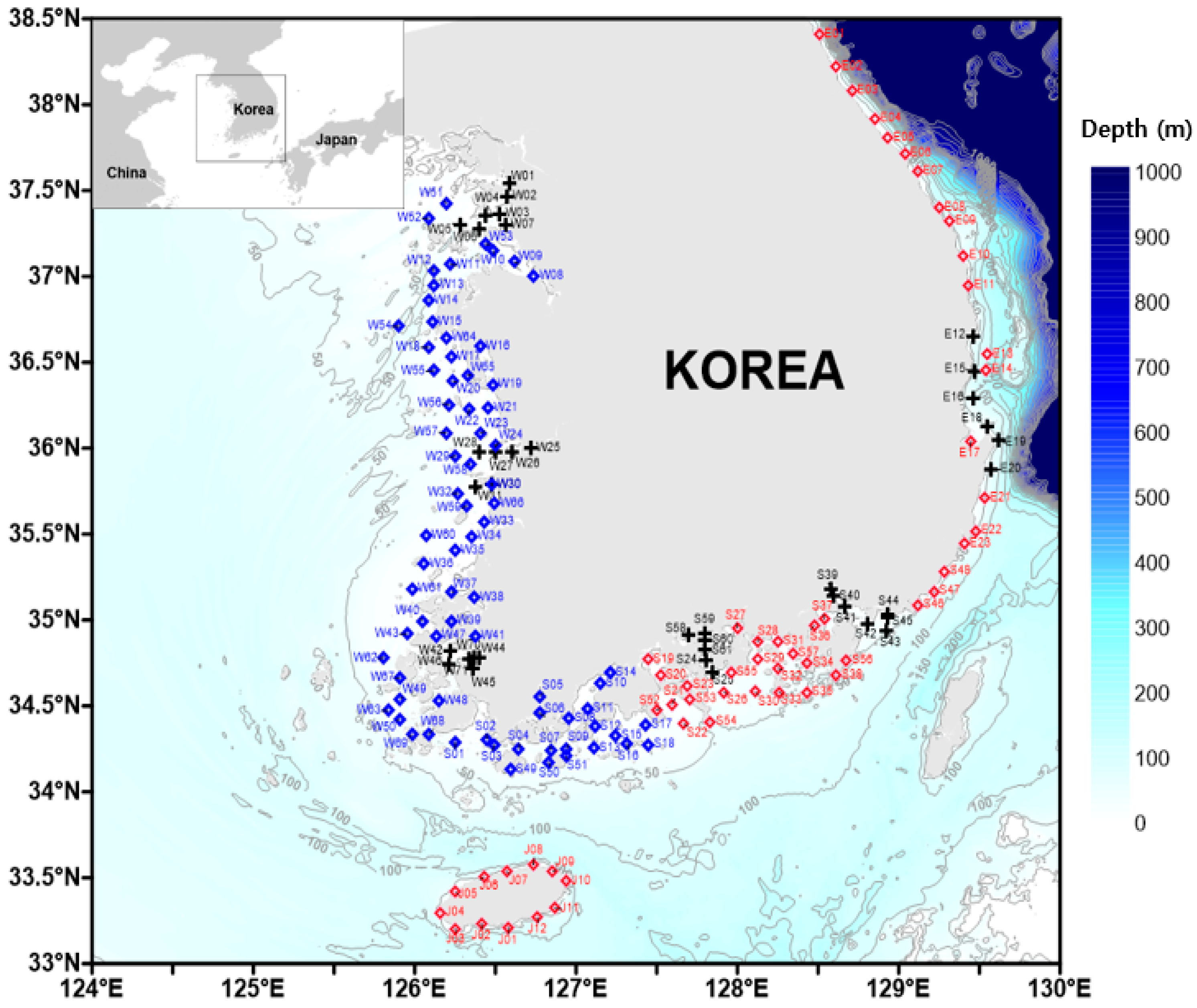
Survey stations and survey items can be found in reference to the history and status of the national marine ecosystem monitoring program in Korea [33]. The data were provided by the Korea Marine Environment Corporation (https://www.koem.or.kr, accessed on 7 March 2022). These data were observed biannually for five years (2015–2019) at the locations presented in Figure 1 during spring and summer, according to the standard manual for basic survey of coastal marine ecosystems [34,35]. In the odd-numbered years (2015, 2017, and 2019), the West Korea coastal zone and southwest coastal zone of Korea were observed (i.e., stations marked with blue diamonds in Figure 1), whereas in the even-numbered years (2016 and 2018), the East Korea coastal zone, southeast coastal zone of Korea, and Jeju coastal zone were observed (i.e., stations marked with red diamonds in Figure 1). However, in 2017, as an exception, the entire coastal area of Korea was observed. Among the observed marine coastal ecosystem data, the physical (i.e., water temperature, salinity, and transparency), chemical (i.e., pH, dissolved oxygen (DO), suspended particulate matter (SPM), particulate organic carbon (POC), particulate organic nitrogen (PON), dissolved silicate (DSi), dissolved inorganic phosphorus (DIP), dissolved inorganic nitrogen (DIN), NO2, NO3, and NH4), and biological (i.e., Chl-a concentration) data were extracted and used in this study. The three categories (i.e., physical, chemical, and biological) included observed data from the surface and bottom layers of each station from 2015 to 2019. However, we only used the surface layer data (water depth of 1 m), with 729 datapoints in total.
The provided raw data consisted of several excel files categorized within a folder for each year. Data preprocessing was performed by reading an excel file into R (version 4.1.2, https://www.r-project.org, accessed on 7 March 2022). We used the R software for all data preprocessing and the data analysis. Because the data in each category were mainly classified by year, they were merged horizontally and then sorted and filtered. Next, we vertically connected the integrated data (i.e., five-year data combined by category) based on the year, season, station, and depth. Consequently, there were 1583 datapoints in total. When the missing pattern was confirmed, the missing rate of the Chl-a concentration data, which was to be used as the target variable, exceeded 30%. This high missing rate caused a problem by lowering the replacement accuracy. To reduce the missing rate of the Chl-a data, we filtered the data based on a depth of 1 m. Consequently, the number of datapoints was 729, and the missing rate of Chl-a data was 0.14%.
2.2. Evaluation of Multiple Imputation (MI) Methods
To replace the missing values of the marine coastal ecosystem observations, we conducted a comparative experiment (Figure 2) to select an appropriate method from several MI methods, which are built in the mice package in R [36]. As shown in Figure 2, the pmm, cart, rf, norm, norm.nob, norm.boot, and norm.predict hyperparameters were varied for the imputation methods. In the imputation phase of Figure 2, m is the number of MI datasets. We generated 20 complete imputed datasets for each of the methods in Figure 2 using the mice package. We used the root mean square error (RMSE) to compare and evaluate the different methods. An RMSE value of zero indicates that the imputed dataset has a perfect fit. The lower the RMSE value, the better the method. We conducted the experiment to determine which method showed the smallest difference between the true and imputed values. Then, we replaced the missing values using the selected method.
In the RMSE of the evaluation phase in Figure 2, n is the number of observations, Ytrue represents the value of the dataset with no missing data, and Yimp represents the value of the imputed complete dataset generated by the MI method in the incomplete dataset with missing values. We used the data presented in Section 3.2 for this experiment. Therefore, we obtained 20 RMSE values for each variable (i.e., input and target variables) in Figure 2.
2.3. Machine Learning Algorithms
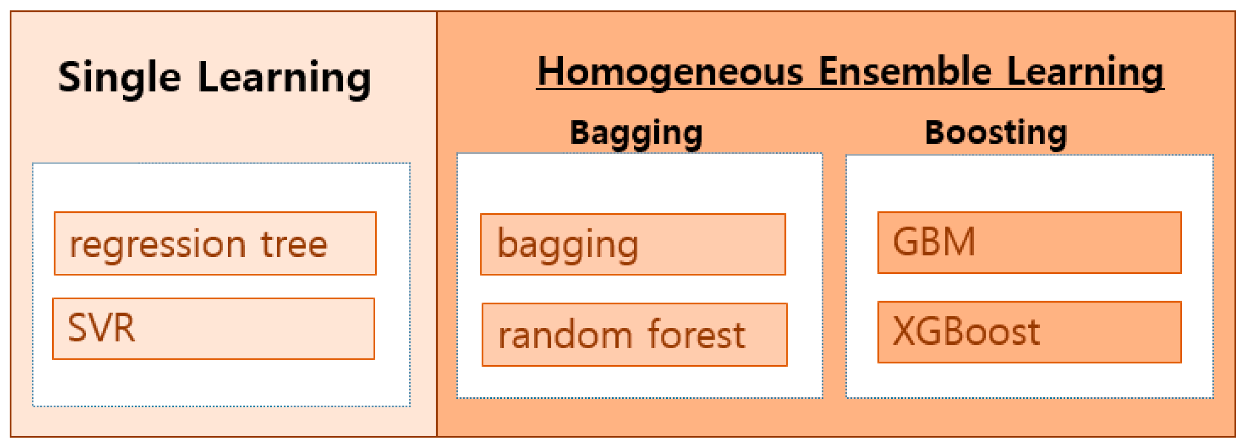
Six machine learning algorithms were used to predict the Chl-a concentration from the marine coastal ecosystem observations. Single learning (regression tree, SVR) using only one model and ensemble learning (boosting, random forest, GBM, and XGBoost) combining multiple models were used (Figure 3). In this study, ensemble learning refers to tree-based learning and the final result was derived by combining several regression trees. An individually trained model is called a weak learner in ensemble learning, which is divided into bagging and boosting techniques depending on whether the weak learners have mutual influence during learning. Bagging is a parallel method in which each model learns independently. It aggregates the final result using an average after combining the results of all the weak learners. Boosting follows a sequential method in which each model learns sequentially to improve the prediction power. Boosting is a technique for synthesizing results by giving weight to a good weak learner when deriving results [37,38,39].
A regression tree is the regression of a decision tree for the prediction of a continuous target variable; the relationship between variables is analyzed using a tree structure, and the analysis encompasses efficient recursive segmentation. A characteristic that significantly increases the homogeneity of the result is set as the partitioning condition during recursive division. The regression tree measures homogeneity with statistics such as variance, standard deviation, and absolute deviation from the mean [40].
SVR is a regression algorithm of support vector machines (SVMs), where an SVM represents an algorithm that finds the optimal linear decision boundary that linearly separates data. In addition to linear classification, an SVM efficiently performs non-linear classification using a technique that maps input data into multidimensional space, called a kernel trick. RBF kernel SVM is the best performing SVM algorithm and is widely used [41].
Bagging is an acronym for bootstrap aggregation and involves combining the outputs of multiple models (e.g., N regression trees) to obtain a generalized output. Bagging uses a bootstrap sampling technique to generate numerous subsets (bags) of the original training dataset with replacement [42]. The average strategy is used for the regression problem, and the majority strategy is used for the classification problem to generalize the ensemble results.
Random forest is an extension of bagging, and it randomly selects both samples and features, while bagging randomly selects only samples. It uses a subset of training samples and features to build multiple base learners (e.g., N regression trees) [38].
A boosting architecture is the generation of sequential hypotheses, where each hypothesis tries to improve or correct the mistakes made in the previous one [38]. GBM is a typical boosting algorithm using gradient descent and is implemented to sequentially learn the residuals using multiple tree models by reducing errors. It is slow and prone to overfitting because of a lack of regulatory functions [43,44].
2.4. Regression Model Accuracy Metrics
Four evaluation metrics—coefficient of determination (R-squared or R2), RMSE, mean absolute error (MAE), and Spearman correlation coefficient—were used to evaluate the performance of the regression model, and the four formulas are shown in Table 1. In artificial intelligence, including machine learning, non-linear models are being preferred over linear models. Therefore, the Spearman’s correlation coefficient, which measures the correlation using ranking, was added as a performance evaluation factor to identify nonlinear relationships in addition to linear relationships. However, in the regression model, indicators of how accurately “to predict” data are crucial. Chicco [46] suggested that R-squared was a more beneficial indicator than symmetric mean absolute percentage error (SMAPE), MAE, mean absolute percentage error (MAPE), mean squared error (MSE), and RMSE. In the formula in Table 1, n is the number of observations, and are the i-th observed value and predicted value of the model, respectively, and is the mean of the observed value. and are the rank of the i-th observed value and predicted value, respectively. The coefficient of determination can be interpreted as the proportion of variation in the target variable, which is explained by the independent variables [46]. R2 has a value between −∞ and 1, and for which a higher value indicates higher accuracy. MAE and RMSE always have non-negative values. The MAE and RMSE values closer to zero imply a higher model accuracy [16,47].
3. Results
3.1. Missing Data Pattern
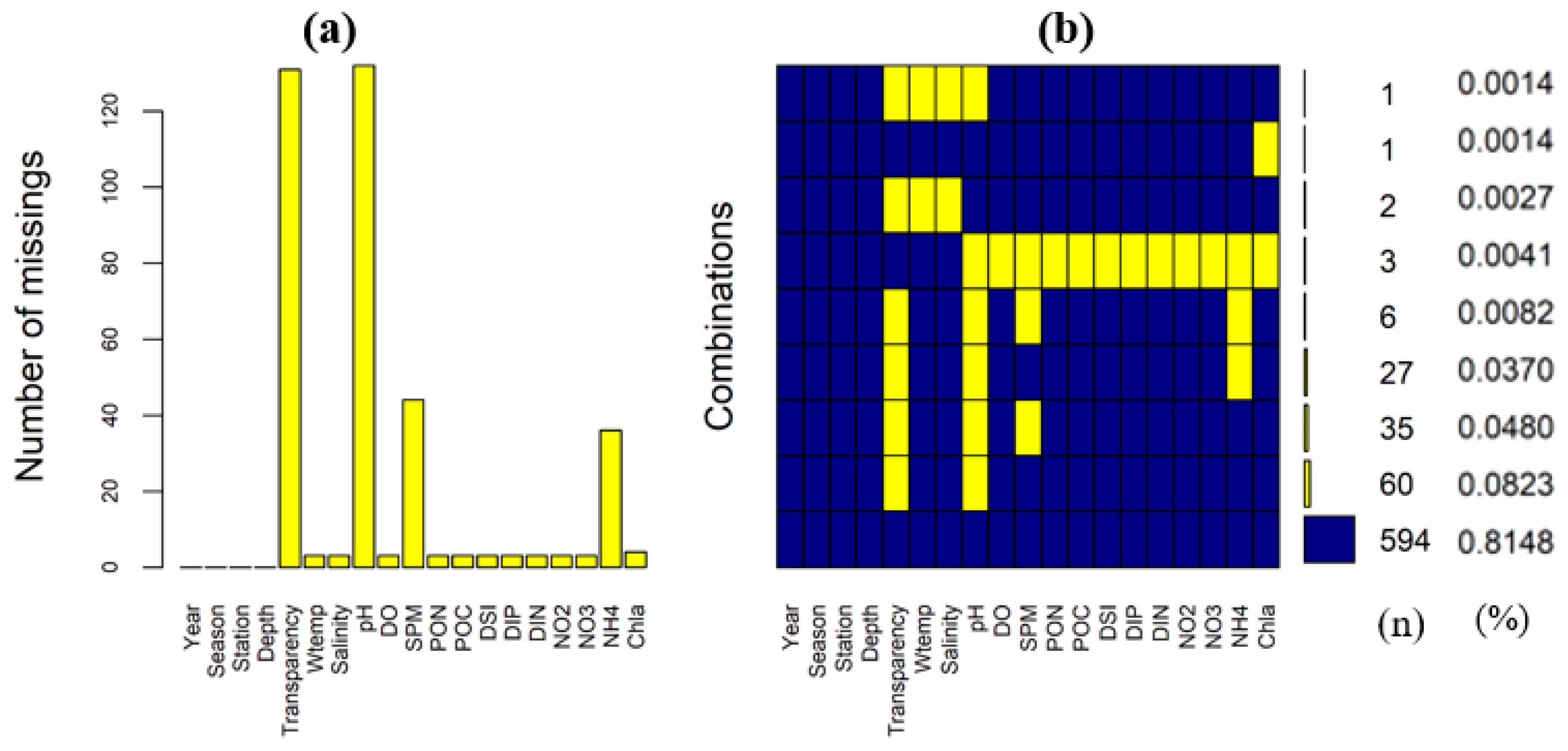
The analyzed data (n = 729) consist of a total of 729 observed datapoints, which are the surface layer (water depth = 1 m) data of physical, chemical, and biological factors along the coastal zone of Korea over five years (2015–2019). They include 15 features, except for the four distinct features of year, season, station, and depth, as shown in Figure 4. Figure 4a represents the number of missing values in each feature and Figure 4b represents the number of missing values through a combination of features and the ratio of missing values. In Figure 4a, the missing values of pH and transparency are high because there were no observations in 2016. In Figure 4b, 594 represents the number of samples without any missing information and 60 represents the number of samples in which pH and transparency are simultaneously missing. Figure 4b presents the Chl-a missing rate (0.0014), which, as the target variable, is significantly below 1%.
3.2. Selection of Multiple Imputation Method
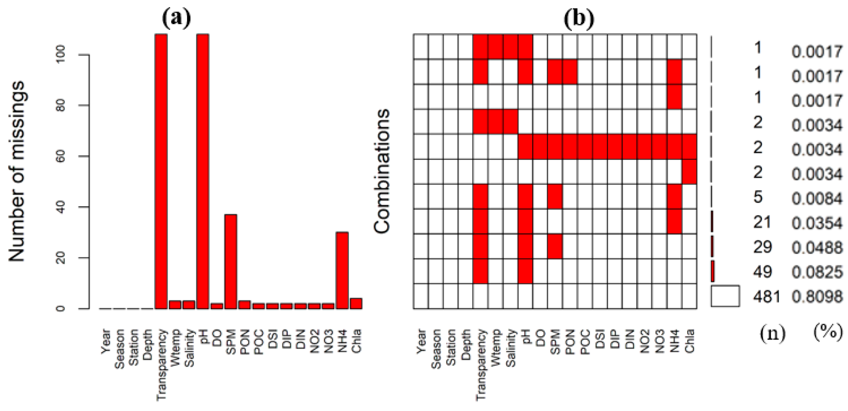
The data without missing information (n = 594) in Figure 4b were considered in the true value dataset. Next, we randomly generated missing values with the proportion of missing values for each variable and variable combinations, as shown in Figure 4b. Figure 5 shows that the experimental dataset (n = 594) was generated with a missing shape and proportion similar to the analysis dataset of Figure 4 (n = 729). Additionally, a boxplot was drawn and analyzed for features with the distribution skewed to over four; the absolute value of skewness was considered so that the results are not distorted for extremely large or small values. Four values (red circles) of Chl-a (skewness: 7.86), SPM (skewness: 9.56), NH4 (skewness: 4.43), and PON (skewness: 7.22) were treated as missing (Supplementary Materials Figure S1).
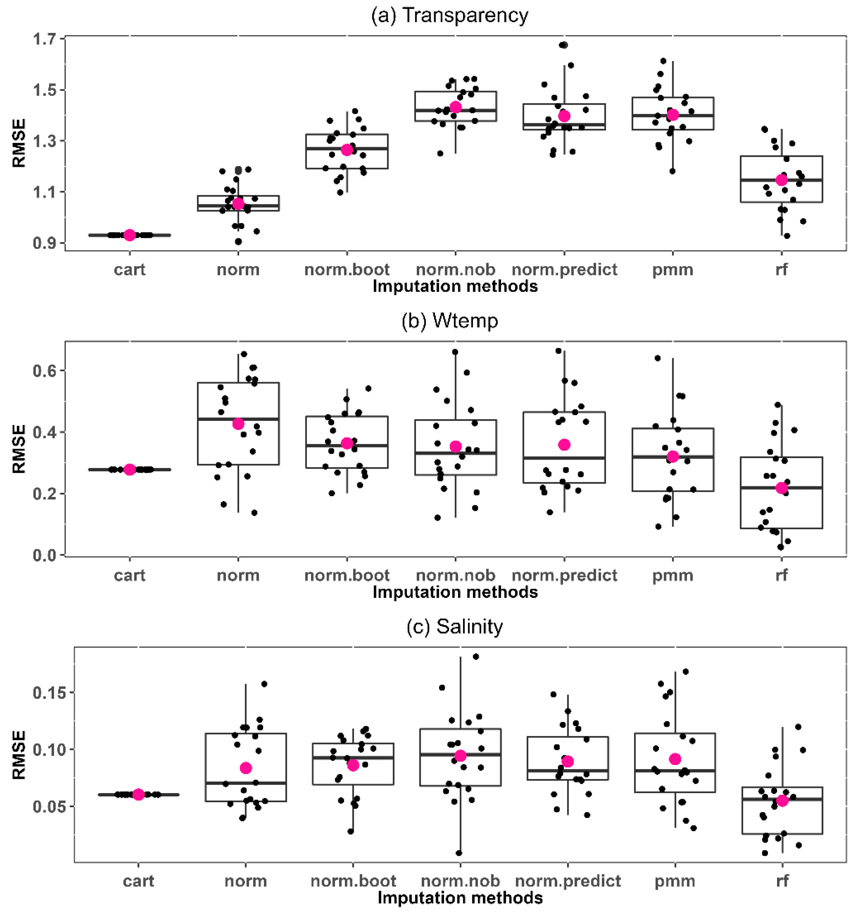
For the experiment in Figure 2, we generated 20 complete imputed datasets from the incomplete dataset (n = 594); thus, 20 RMSE values were derived for each variable, and their distribution is shown as a boxplot. Because seven imputation methods were used, seven boxplots are presented in Figure 6 for each variable. We used the RMSE as an indicator to show the difference between the true and imputed values for each variable. The closer the RMSE value is to 0, the better. Among them, Figure 6 shows the RMSE distribution for transparency, water temperature, and salinity, and the closed pink circle represents the mean. The cart method showed the lowest RMSE among the imputation methods. It was confirmed that the cart method has a small RMSE value for most of the remaining marine water environment features (see Supplementary Materials Figures S2–S5).
3.3. Missing Imputation by Cart Multiple Imputation and Exploratory Data Analysis
For the analyzed data (n = 729) with a ratio of missing information as in Figure 4b, six extreme values were additionally treated as missing. The boxplots were analyzed for features with a large, skewed distribution and an absolute skewness value of 4 or more (absolute skewness value ≥ 4): Chl-a (skewness: 7.76), salinity (skewness: −6.30), SPM (skewness: 9.41), NO3 (skewness: 7.93), NH4 (skewness: 4.49), and PON (skewness: 7.89). In addition, six values—as indicated with red circles—were treated as missing (see Supplementary Materials Figure S6). Multiple imputation was performed using the cart method, as noted in Section 3.2, and the final machine learning dataset (n = 729) was obtained by calculating the average value of 20 complete imputed datasets.
Table 2 shows the maximum, minimum, average, quartile, skewness, kurtosis, and coefficient of variation (CV) for each feature. In particular, the coefficient of variation, which represents the ratio of the standard deviation to the mean, can compare variations between features with different units. Therefore, pH (CV = 0.02) had the smallest variation, and PON (CV = 1.77) had the largest variation. Skewness gives information about the distribution asymmetry and direction of outliers, and kurtosis indicates how much the data is concentrated on the mean. Skewness decreased the asymmetry, compared with that from before the missing imputation: Chl-a (skewness: 2.29), salinity (skewness: −2.94), SPM (skewness: 1.72), NO3 (skewness: 3.36), NH4 (skewness: 3.53), and PON (skewness: 5.06). The DIN (kurtosis: 52.36) and PON (kurtosis: 35.58) values were more concentrated around the mean compared with other features, as highlighted by the larger kurtosis values.
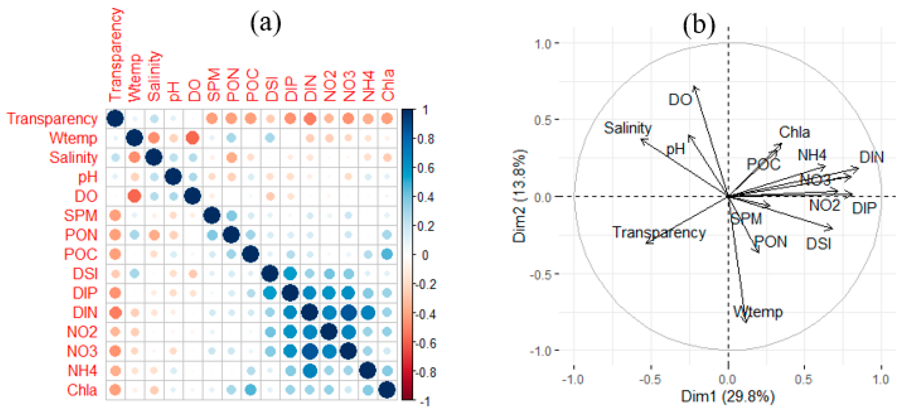
For the normality test of each feature, the Shapiro test was performed, which confirmed that all p-values were significantly small and that not all features were normally distributed. Therefore, the Spearman’s correlation analysis, a non-parametric correlation analysis, was performed to understand the correlation between variables (features). The darker the blue color, the greater the positive correlation, and the darker the red color, the greater the negative correlation (Figure 6a). Chl-a, POC (ρ = 0.47), NH4 (ρ = 0.36), NO2 (ρ = 0.33), DIP (ρ = 0.32), DIN (ρ = 0.31), PON (ρ = 0.28), NO3 (ρ = 0.18), DSi (ρ = 0.11), pH (ρ = 0.11), and SPM (ρ = 0.10) showed a significant (p < 0.05) positive correlation, whereas transparency (ρ = −0.42) and salinity (ρ = −0.25) showed a significant (p < 0.05) negative correlation. We performed a principal component analysis (PCA) for exploratory data analysis. The loading plot of PCA shows how strongly each variable influences a principal component and the correlation between variables (Figure 7b). The two principal components accounted for 43.6% of the total variance of the data. Nutrients such as DIN, DIP, NO3, and NO2 strongly influenced Dim1, while physical environmental information, such as water temperature, DO, pH, and salinity, more strongly influenced Dim2. POC and NH4 are positively correlated with Chl-a because the two variable vectors were similar, forming a small angle between them. Moreover, transparency was negatively correlated with Chl-a because they formed a large angle close to 180°, as it was located on the opposite side of Chl-a (Figure 7b).
3.4. Distribution of Features before and after Imputation
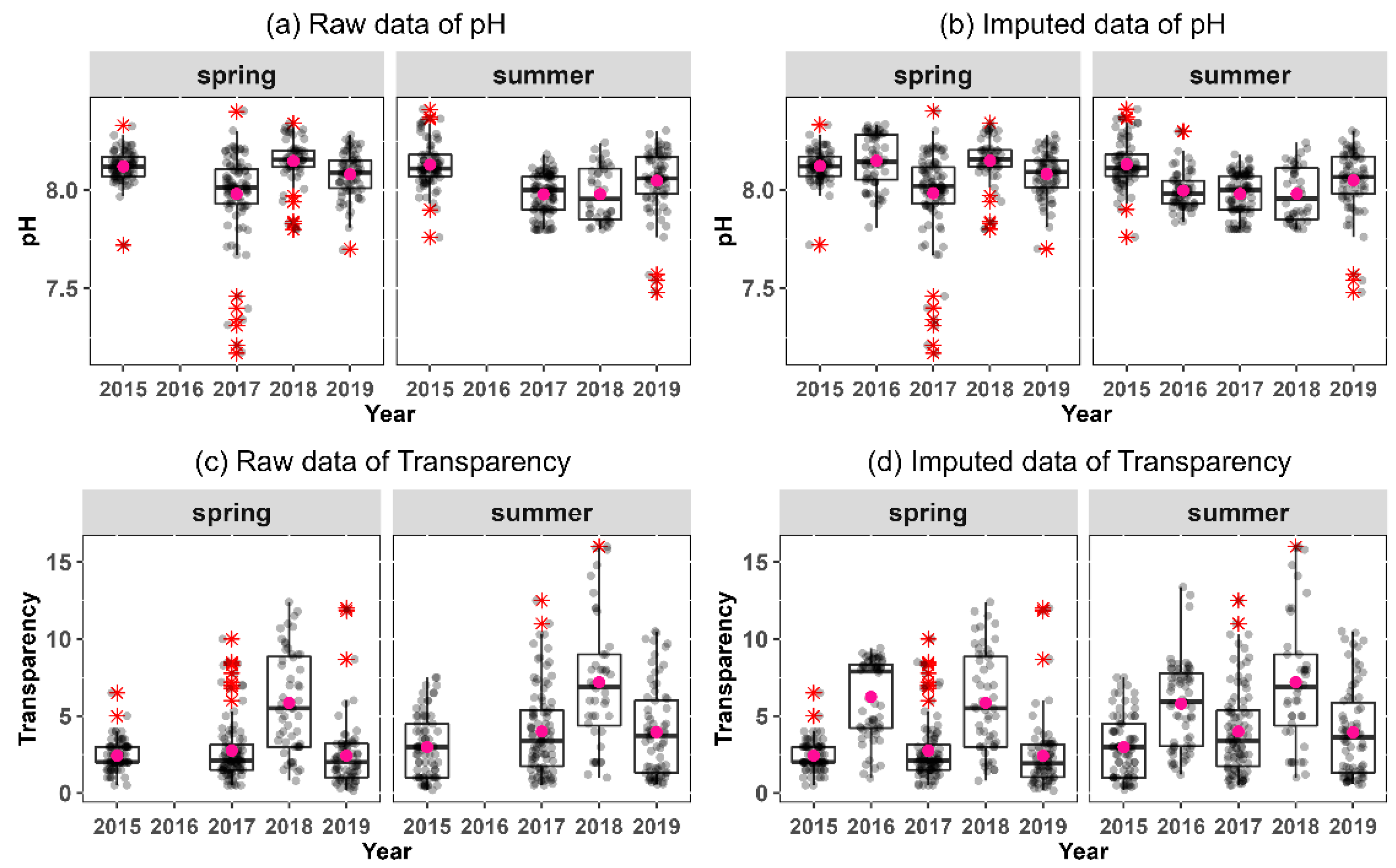
Figure 8 shows the results before and after imputation for pH and transparency with missing values from the spring and summer 2016 surveys. During the 2015–2019 survey period, the East Korea coastal zone, southeast coastal zone of Korea, and Jeju coastal zone, were observed in 2016 and 2018. The pH imputed in the spring of 2016 ranged from 7.81–8.33 (mean 8.15), which was similar to the 7.80–8.34 range (mean 8.15) for the pH observed in the spring of 2018. The pH imputed in the summer of 2016 was 7.83–8.30 (mean 8.00), which was similar to the pH observed in the summer of 2018 (7.80–8.24, with a mean of 7.98), but the mean was slightly higher. The imputed transparency from the spring of 2016 was 0.97–9.41 (mean 6.24 m), which was narrower than the observed transparency from the spring of 2018 (0.80–12.40, with a mean of 5.86 m); the average transparency was somewhat higher. In contrast, the imputed transparency from the summer of 2016 was 1.20–13.38 (mean 5.79 m), narrower than the observed transparency from the summer of 2018 (1.00–16.00, with a mean of 7.20 m); however, the average transparency was low.
3.5. Performance Evaluation of Machine Learning Model
The R software (version 4.1.2) was used for all machine learning predictions. We used six machine learning algorithms (regression tree, SVR, bagging, random forest, GBM, and XGBoost) to predict the concentration of Chl-a. The dataset (n = 729) contains fifteen features, as shown in Table 2. It has different scales, that is, the range of water temperature was between 9.22 and 30.28 °C while the Chl-a concentration was between 0.03 and 14.58 μg/L. To reduce the complexity of the data and ensure that the datasets were of the same scale, the data was normalized to values between 0 and 1 using min–max scaling [48]. All algorithms were run under 10-fold cross-validation (CV), which is a powerful tool to avoid the overfitting of data [48]. During CV, the data were divided into ten sets, with nine sets used for training and one set for testing; this process was repeated ten times using different data for each testing phase We used four measures (i.e., MAE, RMSE, Spearman’s correlation coefficient, and R2) for the predictive model performance evaluation. Ten models trained through the CV process were created, and performance measures were calculated using the predicted and actual values. The algorithms were optimized by adjusting the hyperparameters as follows: regression tree algorithm (i.e., rpart in R), minsplit = 16, maxdepth = 9, and cp = 0.01; SVR algorithm (i.e., SVM in R), cost = 4, gamma = 0.125, epsilon = 0.2; bagging algorithm (i.e., bagging in R), nbagg = 54, coob = TRUE, minsplit = 16, maxdepth = 9, cp = 0.01; random forest algorithm (i.e., randomForest in R), ntree = 400, mtry = 4; GBM algorithm (i.e., gbm in R), distribution = “gaussian,” n.trees = 1500, interaction.depth = 8, shrinkage = 0.01, n.minobsinnode = 5, bag.fraction = 0.5; XGBoost algorithm (i.e., xgboost in R), max.depth = 8, eta = 0.06, nrounds = 5000, early_stop_rounds = 1000, colsample_bytree = 0.7, subsample = 0.95. Table 3 shows the mean of the performance measurements.
Based on the training and test datasets in CV, we calculated the optimal parameter combination of each algorithm several times. The RMSE showed good performance in the order of XGBoost (0.090), random forest (0.093), SVR (0.094), GBM (0.094), bagging (0.099), and regression tree (0.107). R2 showed good performance in the order of XGBoost (0.520), random forest (0.500), SVR (0.493), GBM (0.471), bagging (0.413), and regression tree (0.308). MAE showed good performance in the order of SVR (0.061), XGBoost (0.062), random forest (0.063), GBM (0.065), bagging (0.069), and regression tree (0.073). The Spearman correlation coefficient appeared in the order of SVR (0.744), random forest (0.731), XGBoost (0.720), GBM (0.698), bagging (0.658), and regression tree (0.557). Overall, tree-based ensemble learning was superior to tree-based single learning; in particular, XGBoost outperformed the other models. Moreover, single learning SVR showed good performance in MAE and Spearman’s correlation coefficient.
3.6. Feature Importance
Unlike linear regression models, most machine learning models do not provide sufficient information about the relationships between variables (i.e., features), but instead allow us to estimate which variables play an essential role in the predictive performance of the target variable through feature importance. Figure 9 shows the feature importance in the model in which the third R2 value of XGBoost’s 10-fold cross-validation showed a value of 0.719. The important feature ranking is shown in order of POC and DO. However, DIN, SPM, and some others have low feature rankings and show a weak influence in predicting concentrations of Chl-a.
4. Discussion
This study constructed a high-quality dataset for machine learning by appropriately processing the missing values in field observation data. The existence of missing data is shown in Figure 4. Six additional values were treated as missing, as mentioned in Section 3.3, to avoid distorting the results because of extreme values. The missing data were replaced using the cart method. Because the existing observation values are known, changes in the imputed values can be identified (Table 4), especially for the six added values. Referring to the quartile values in Table 2 and looking at the imputed values of Chl-a, salinity, NO3, NH4, PON, and SPM, it can be observed that the imputed values of Chl-a, NO3, NH4, and PON were larger than the 3rd quartile. The minimal salinity values were imputed with values below the 1st quartile. However, the SPM of the sample (i.e., summer 2017 and W50 station), in which two features (i.e., SPM and PON) were simultaneously missing, was imputed with a value below the median. The extreme values were clearly replaced with relaxed values. It is ill-advised to use an imputed value of a multiple imputation method after treating such extreme values as missing; it may be more appropriate to use the original values for regional and seasonal sparsity. In addition, it is necessary to track which changes in the machine learning model result from changes in this value; however, this is beyond the scope of our study. Although this study and Noh [30] claim that the cart method is superior to many imputation methods, Chhabra [49] stated that the norm (Bayesian regression) method was superior, Jadhav [50] stated that the KNN method was excellent, and Kim [51] suggested that imputation methods should be evaluated by both the imputation and model performances. Thus, we cannot argue if one imputation method is superior overall because the data components, missing rates, and evaluation criteria are not similar. However, it is necessary to select an imputation method suitable for the situation according to the characteristics of the data to eliminate any biases that may arise from conventional missing data removal.
The features with the highest missing rates were pH and transparency, which had no observations during the spring and summer of 2016 (Figure 4a and Figure 8a,c). Multiple imputation methods for machine learning replaced the missing values, but the validation of the imputed values cannot be discussed when the true value is unknown. However, we compared it with 2018 data observed in a similar area (Figure 8). The imputed pH in the spring of 2016 showed a similar distribution and average value to the pH observed in the spring of 2018, but the interquartile range tended to be wider. In contrast, the imputed pH in the summer of 2016, instead of spring, had a narrower interquartile range. However, transparency showed the opposite trend to pH. This difference may arise from the small sample size and the estimation, which excluded temporal and spatial characteristics. Therefore, after the continuous accumulation of more observational data, the comparative and verification studies on the imputed data, in consideration of regional characteristics, can be positioned as an excellent alternative to replace the missing field data, which will inevitably occur structurally in the future.
The initial research direction for predicting the Chl-a concentration included correlation analysis, multiple regression analysis, and principal component regression analysis, using water quality environment data to predict Chl-a concentration or to identify critical influencing factors [52,53]. However, the advent of machine learning has led to improved prediction performance by using various machine learning and deep learning methods applicable to complex and non-linear relationships, moving away from the classic multiple regression analysis for Chl-a concentration prediction. When predicting the concentration of Chl-a in a freshwater environment, forecast performance was improved using weather variables (e.g., average temperature, sunshine, rainfall, inflow, and outflow) in addition to water quality variables (e.g., water temperature, pH, electric conductivity, DO, and total organic carbon) [16]. In other studies on Chl-a concentration and algal bloom prediction using machine learning methods, explanatory variables belonging to four different categories (chemical, biological, meteorological, and hydrodynamic) have been used (Table 5). In particular, harmful algal blooms (HAB) occur when wind and water currents are favorable or in sluggish water circulation or in a marine environment suitable for red algae overgrowth because of sunlight, water temperature, salinity, and nutrients [54,55]. Table 5 includes studies to predict Chl-a concentrations and algal blooms using machine learning in freshwater [11,13,14,32,56] and seawater [16,17]. The physical category includes water temperature and salinity, which are the most basic properties of water, along with transparency, such as Secchi depth. The chemical category includes DO, BOD, COD, SS, and TOC (particulate organic carbon + dissolved organic carbon), which are indicators of water pollution, along with nutrients such as nitrogen, phosphorus, and silicon: TDN, TDP, NO2, NO3, NH4, NH3, TN, and TP (Table 5). The biological category includes phytoplankton and zooplankton abundance, which are factors of predation relationship; the meteorological category includes temperature, precipitation, wind, solar radiation, etc.; and the hydrodynamic category includes water flow, water level, flux, discharge rate, etc.
Except for decision trees, most of the machine learning models are not easily interpretable. However, it is only possible to know the importance score of features (i.e., the higher score, the more large effect) to the predictive power of a given model between the input features and the target variable, as shown in Figure 9. Unlike the linear regression model, we may not know whether or how the predictor variable affects the target variable in the positive or negative direction.
Four evaluation criteria (MAE, RMSE, Spearman’s correlation coefficient, and R2) were used for model performance evaluation. In particular, R2 provided more information than MAE and RMSE in regression model evaluation [46]. XGBoost outperformed other models in R2 and RMSE. To predict the Chl-a concentration, only the physical and chemical features in Table 5 were used; thus, the prediction performance was not as high. Improving the machine learning model accuracy requires large and diverse datasets [1]. Therefore, by considering the biological (e.g., phytoplankton abundance and zooplankton abundance), meteorological (e.g., temperature and precipitation), and hydrodynamic categories (e.g., tide), and by accumulating more data than previously used, it seems that the predictive performance can be improved.
During the survey period from 2015 to 2019, observations were conducted twice a year (spring and summer). In particular, the western region was observed during odd-numbered years and the eastern region was observed during even-numbered years. There existed a limit in the reflecting time series characteristics of the data, and it did not reflect the temporal characteristics. However, for future Chl-a concentration research, it is necessary to accumulate and use coastal environment data for longer periods to reflect the temporal characteristics. In addition, if the various features mentioned in Table 5 are collected and merged, the prediction accuracy can be improved with a multivariate time series study, and then meaningful regional and seasonal interpretations can be derived. We expect that this process and its results will be used as a generalized methodology to apply machine learning to marine environment data.
5. Conclusions
The dataset used in this study was based on surface layer data (n = 729) observed during the spring and summer from 2015 to 2019 in the coastal zone of Korea. We attempted to predict the concentration of Chl-a, which is one of the critical indicators of change in the marine environment, using machine learning, and after replacing the missing values with multiple imputation. First, to find the most suitable multiple imputation method, we conducted a comparison experiment using seven multiple imputation methods (pmm, cart, rf, norm, norm.nob, norm.boot, and norm.predict). The most appropriate method for this study was found to be the cart method. Second, we generated machine learning models for Chl-a concentration prediction using six machine learning algorithms (regression tree, SVR, bagging, random forest, GBM, and XGBoost) rather than linear regression because of the complexity and non-linearity of the ecosystem. A 10-fold cross-validation was performed to estimate the performance of the models. XGBoost outperformed the other models. SVR also showed a good predictive performance. In addition, POC had the greatest influence on the prediction of Chl-a concentration and DO also showed potential. The results of our study suggest that our overall process and techniques can be generalized to make biological feature (e.g., phytoplankton abundance, zooplankton abundance, and Chl-a concentration) predictions and derive important influencing features.
The Chl-a concentration prediction accuracy is low in our study because the meteorological and hydrodynamic categories were not considered in aquatic ecosystem situations; only physical and chemical features were used. For a more accurate prediction of biological features using machine learning or deep learning, it is necessary to collect long-term field observation data considering various features presented in Table 5.
Supplementary Materials
The following supporting information can be downloaded at: https://www.mdpi.com/article/10.3390/w14121862/s1, Figure S1: Distribution of features with absolute skewness ≥ 4 of the dataset (n = 594) without missing values; Figure S2. RMSE distribution for pH, DO, and SPM; Figure S3. RMSE distribution for PON, POC, and DSI; Figure S4. RMSE distribution for DIP, DIN, and NO2; Figure S5. RMSE distribution for NO3, NH4, and Chlorophyll-a; Figure S6. Distribution of features with absolute skewness ≥ 4 of the dataset (n = 729) with missing values
Author Contributions
Conceptualization, S.-H.H. and H.Y.S.; data curation, H.-R.K.; validation, H.Y.S.; software, H.-R.K.; visualization, H.-R.K. and M.-T.K.; supervision, S.-H.H. and M.-T.K.; writing—original draft preparation, H.-R.K.; writing—review and editing, H.Y.S., M.-T.K. and S.-H.H. All authors have read and agreed to the published version of the manuscript.
Funding
This research was a part of the project titled “Research center for fishery resource management based on the information and communication technology” (2022, grant number 20180384), funded by the Ministry of Oceans and Fisheries, Korea.
Institutional Review Board Statement
Not applicable.
Informed Consent Statement
Not applicable.
Data Availability Statement
Not applicable.
Acknowledgments
We would like to thank the Marine Ecology Team of the Korea Marine Environment Management Corporation for providing the coastal ecosystem DB data.
Conflicts of Interest
The authors declare no conflict of interest.
References
- Rajkomar, A.; Dean, J.; Kohane, I. Machine learning in medicine. N. Engl. J. Med. 2019, 380, 1347–1358. [Google Scholar] [CrossRef] [PubMed]
- Jordan, M.I.; Mitchell, T.M. Machine learning: Trends, perspectives, and prospects. Science 2015, 349, 255–260. [Google Scholar] [CrossRef] [PubMed]
- Gudivada, V.; Apon, A.; Ding, J. Data quality considerations for big data and machine learning: Going beyond data cleaning and transformations. Int. J. Adv. Softw. 2017, 10, 1–20. [Google Scholar]
- Kim, E.D.; Ko, S.K.; Son, S.C.; Lee, B.T. Technical Trends of Time-Series Data Imputation. Electron. Telecommun. Trends 2021, 36, 145–153. [Google Scholar] [CrossRef]
- El-Masri, M.M.; Fox-Wasylyshyn, S.M. Missing data: An introductory conceptual overview for the novice researcher. Can. J. Nurs. Res. 2005, 37, 156–171. [Google Scholar]
- Allison, P.D. Multiple imputation for missing data: A cautionary tale. Sociol. Methods Res. 2000, 28, 301–309. [Google Scholar] [CrossRef] [Green Version]
- Patrician, P.A. Multiple imputation for missing data. Res. Nurs. Health 2002, 25, 76–84. [Google Scholar] [CrossRef]
- Emmanuel, T.; Maupong, T.; Mpoeleng, D.; Semong, T.; Mphago, B.; Tabona, O. A survey on missing data in machine learning. J. Big Data 2021, 8, 140. [Google Scholar] [CrossRef]
- Barnard, J.; Meng, X.L. Applications of multiple imputation in medical studies: From AIDS to NHANES. Stat. Methods Med. Res. 1999, 8, 17–36. [Google Scholar] [CrossRef]
- Vilas, L.G.; Spyrakos, E.; Palenzuela, J.M.T. Neural network estimation of chlorophyll a from MERIS full resolution data for the coastal waters of Galician rias (NW Spain). Remote Sens. Environ. 2011, 115, 524–535. [Google Scholar] [CrossRef]
- Park, Y.; Cho, K.H.; Park, J.; Cha, S.M.; Kim, J.H. Development of early-warning protocol for predicting chlorophyll-a concentration using machine learning models in freshwater and estuarine reservoirs, Korea. Sci. Total Environ. 2015, 502, 31–41. [Google Scholar] [CrossRef] [PubMed]
- Hartnett, M.; Nash, S. Modelling nutrient and chlorophyll_a dynamics in an Irish brackish waterbody. Environ. Model. Softw. 2004, 19, 47–56. [Google Scholar] [CrossRef] [Green Version]
- Lee, S.M.; Park, K.D.; Kim, I.K. Comparison of machine learning algorithms for Chl-a prediction in the middle of Nakdong River (focusing on water quality and quantity factors). J. Korean Soc. Water Wastewater 2020, 34, 277–288. [Google Scholar] [CrossRef]
- Shin, Y.; Kim, T.; Hong, S.; Lee, S.; Lee, E.; Hong, S.; Heo, T.Y. Prediction of chlorophyll-a concentrations in the Nakdong River using machine learning methods. Water 2020, 12, 1822. [Google Scholar] [CrossRef]
- Cao, Z.; Ma, R.; Duan, H.; Pahlevan, N.; Melack, J.; Shen, M.; Xue, K. A machine learning approach to estimate chlorophyll-a from Landsat-8 measurements in inland lakes. Remote Sens. Environ. 2020, 248, 111974. [Google Scholar] [CrossRef]
- Yu, P.; Gao, R.; Zhang, D.; Liu, Z.-P. Predicting coastal algal blooms with environmental factors by machine learning methods. Ecol. Indic. 2021, 123, 107334. [Google Scholar] [CrossRef]
- Amorim, F.; Rick, J.; Lohmann, G.; Wiltshire, K. Evaluation of Machine Learning Predictions of a Highly Resolved Time Series of Chlorophyll-a Concentration. Appl. Sci. 2021, 11, 7208. [Google Scholar] [CrossRef]
- Baek, Y.M.; Park, R.S. Missing Data Analysis Using R; Hannara Academy Press: Seoul, Korea, 2021; pp. 110–114. [Google Scholar]
- Rubin, D.B. An overview of multiple imputation. In Proceedings of the Survey Research Methods Section of the American Statistical Association, Princeton, NJ, USA, August 1998; Citeseer. pp. 79–84. [Google Scholar]
- Zhang, Z. Multiple imputation with multivariate imputation by chained equation (MICE) package. Ann. Transl. Med. 2016, 4, 30. [Google Scholar] [CrossRef]
- Yun, S.C. Imputation of missing values. J. Prev. Med. Public Health 2004, 37, 209–211. [Google Scholar]
- Alruhaymi, A.Z.; Kim, C.J. Why Can Multiple Imputations and How (MICE) Algorithm Work? Open J. Stat. 2021, 11, 759–777. [Google Scholar] [CrossRef]
- Kim, J.H. A Study on the Multiple Imputation of Missing Values: Focus on Fine Dust Data. Soc. Converg. Knowl. Trans. 2020, 8, 149–156. [Google Scholar] [CrossRef]
- Murray, J.S. Multiple Imputation: A Review of Practical and Theoretical Findings. Stat. Sci. 2018, 33, 142–159. [Google Scholar] [CrossRef] [Green Version]
- Flexible Imputation of Missing Data (Second Edition). Available online: https://stefvanbuuren.name/fimd/ (accessed on 5 March 2022).
- White, I.R.; Royston, P.; Wood, A.M. Multiple imputation using chained equations: Issues and guidance for practice. Stat. Med. 2011, 30, 377–399. [Google Scholar] [CrossRef] [PubMed]
- Van Buuren, S.; Groothuis-Oudshoorn, K. mice: Multivariate imputation by chained equations in R. J. Stat. Softw. 2011, 45, 1–67. [Google Scholar] [CrossRef] [Green Version]
- Azur, M.J.; Stuart, E.A.; Frangakis, C.; Leaf, P.J. Multiple imputation by chained equations: What is it and how does it work? Int. J. Methods Psychiatr. Res. 2011, 20, 40–49. [Google Scholar] [CrossRef]
- Iterative Imputation for Missing Values in Machine Learning. Available online: https://machinelearningmastery.com/iterative-imputation-for-missing-values-in-machine-learning/ (accessed on 7 March 2022).
- Noh, J.H. Machine Learning Models and Missing Data Imputation Methods in Predicting the Progression of IgA Nephropathy. Master’s Thesis, The Graduate School Seoul National University, Seoul, Korea, February 2015. [Google Scholar]
- Kang, B.K.; Park, J.S. Effect of input variable characteristics on the performance of an ensemble machine learning model for algal bloom prediction. J. Korean Soc. Water Wastewater 2021, 35, 417–424. [Google Scholar] [CrossRef]
- Kim, J.H.; Shin, J.-K.; Lee, H.; Lee, D.H.; Kang, J.-H.; Cho, K.H.; Lee, Y.-G.; Chon, K.; Baek, S.-S.; Park, Y. Improving the performance of machine learning models for early warning of harmful algal blooms using an adaptive synthetic sampling method. Water Res. 2021, 207, 117821. [Google Scholar] [CrossRef]
- Kim, Y.N.; Yoo, J.K.; Yeo, J.W.; Kho, B.S.; Hwang, I.S. History and Status of the National Marine Ecosystem Monitoring Program in Korea. Sea J. Korean Soc. Oceanogr. 2019, 24, 49–53. [Google Scholar]
- Korea Marine Environment Management Corporation (KOEM). Available online: http://koem.or.kr/ (accessed on 7 March 2022).
- Marine Environment Information Portal (MEIS). Available online: http://meis.go.kr/ (accessed on 7 March 2022).
- Package ‘Mice’. Available online: https://cran.r-project.org/web/packages/mice/mice.pdf (accessed on 7 March 2022).
- Rincy, T.N.; Gupta, R. Ensemble Learning Techniques and its Efficiency in Machine Learning: A Survey. In Proceedings of the 2nd International Conference on Data, Engineering and Applications (IDEA), Bhopal, India, 28–29 February 2020; pp. 1–6. [Google Scholar] [CrossRef]
- Schapire, R.E. The Boosting Approach to Machine Learning: An Overview. In Nonlinear Estimation and Classification; Lecture Notes in Statistics; Denison, D.D., Hansen, M.H., Holmes, C.C., Mallick, B., Yu, B., Eds.; Springer: New York, NY, USA, 2003; Volume 171, pp. 149–171. [Google Scholar]
- Yang, X.; Wang, Y.; Byrne, R.; Schneider, G.; Yang, S. Concepts of Artificial Intelligence for Computer-Assisted Drug Discovery. Chem. Rev. 2019, 119, 10520–10594. [Google Scholar] [CrossRef] [Green Version]
- Chung, D.H.; Yun, J.S.; Yang, S.M. Machine Learning for Predicting Entrepreneurial Innovativeness. Asia-Pac. J. Bus. Ventur. Entrep. 2021, 16, 73–86. [Google Scholar]
- Yuvaraj, P.; Murthy, A.R.; Iyer, N.R.; Sekar, S.; Samui, P. Support vector regression based models to predict fracture characteristics of high strength and ultra high strength concrete beams. Eng. Fract. Mech. 2013, 98, 29–43. [Google Scholar] [CrossRef]
- Nti, I.K.; Adekoya, A.F.; Weyori, B.A. A comprehensive evaluation of ensemble learning for stock-market prediction. J. Big Data 2020, 7, 1–40. [Google Scholar] [CrossRef]
- Mitchell, R.; Frank, E. Accelerating the XGBoost algorithm using GPU computing. PeerJ Comput. Sci. 2017, 3, e127–e163. [Google Scholar] [CrossRef]
- Choi, S.; Kim, C. The Empirical Evaluation of Machine Learning Models Predicting Round-Trip Time in Cellular Network. In Proceedings of the 2021 International Conference on Information and Communication Technology Convergence (ICTC), Jeju Island, Korea, 20–22 October 2021; pp. 1374–1376. [Google Scholar] [CrossRef]
- Chen, T.; Guestrin, C. XGBoost: A scalable tree boosting system. In Proceedings of the 22nd Acm Sigkdd International Conference on Knowledge Discovery and Data mining, San Francisco, CA, USA, 13–17 August 2016. [Google Scholar]
- Chicco, D.; Warrens, M.J.; Jurman, G. The coefficient of determination R-squared is more informative than SMAPE, MAE, MAPE, MSE and RMSE in regression analysis evaluation. PeerJ Comput. Sci. 2021, 7, e623. [Google Scholar] [CrossRef] [PubMed]
- Ray, S.; Rahman, M.; Haque, M.; Hasan, M.W.; Alam, M.M. Performance evaluation of SVM and GBM in predicting compressive and splitting tensile strength of concrete prepared with ceramic waste and nylon fiber. J. King Saud Univ. Eng. Sci. 2021, in press. [Google Scholar] [CrossRef]
- Kooh, M.R.R.; Thotagamuge, R.; Chau, Y.-F.C.; Mahadi, A.H.; Lim, C.M. Machine learning approaches to predict adsorption capacity of Azolla pinnata in the removal of methylene blue. J. Taiwan Inst. Chem. Eng. 2022, 132, 104134. [Google Scholar] [CrossRef]
- Chhabra, G.; Vashisht, V.; Ranjan, J. A Comparison of Multiple Imputation Methods for Data with Missing Values. Indian J. Sci. Technol. 2017, 10, 1–7. [Google Scholar] [CrossRef]
- Jadhav, A.; Pramod, D.; Ramanathan, K. Comparison of Performance of Data Imputation Methods for Numeric Dataset. Appl. Artif. Intell. 2019, 33, 913–933. [Google Scholar] [CrossRef]
- Kim, W.; Cho, W.; Choi, J.; Kim, J.; Park, C.; Choo, J. A Comparison of the Effects of Data Imputation Methods on Model Performance. In Proceedings of the 2019 21st International Conference on Advanced Communication Technology (ICACT), PyeongChang, Korea, 17–20 February 2019. [Google Scholar] [CrossRef]
- Amdevýren, H.; Demýr, N.; Kanik, A.; Keskýn, S. Use of principal component scores in multiple linear regression models for prediction of Chlorophyll-a in reservoirs. Ecol. Model. 2005, 181, 581–589. [Google Scholar] [CrossRef]
- Cho, K.H.; Kang, J.-H.; Ki, S.J.; Park, Y.; Cha, S.M.; Kim, J.H. Determination of the optimal parameters in regression models for the prediction of chlorophyll-a: A case study of the Yeongsan Reservoir, Korea. Sci. Total Environ. 2009, 407, 2536–2545. [Google Scholar] [CrossRef]
- National Institute of Fisheries Science (NIFS). Available online: https://www.nifs.go.kr/red/info_1.red (accessed on 2 April 2022).
- National Oceanic and Atmospheric Administration (NOAA). Available online: https://oceanservice.noaa.gov/facts/why_habs.html (accessed on 3 June 2022).
- Yi, H.-S.; Lee, B.; Park, S.; Kwak, K.-C.; An, K.-G. Prediction of short-term algal bloom using the M5P model-tree and extreme learning machine. Environ. Eng. Res. 2019, 24, 404–411. [Google Scholar] [CrossRef]
Figure 1.
Map showing the sampling stations in the coastal zone of Korea. Blue and red diamonds represent stations analyzed during odd and even years, respectively, over five years (2015–2019). The cross marks indicate estuaries.
Figure 1.
Map showing the sampling stations in the coastal zone of Korea. Blue and red diamonds represent stations analyzed during odd and even years, respectively, over five years (2015–2019). The cross marks indicate estuaries.

Figure 2.
Multiple imputation comparison of seven different methods. Abbreviations: RMSE, root mean square error; pmm, predictive mean matching; norm, Bayesian linear regression; norm.nob, linear regression ignoring model error; norm.boot, linear regression using bootstrap; norm.predict, linear regression, predicted values; cart, classification and regression trees; rf, random forest imputations [36].

Figure 3.
Machine learning algorithms. Abbreviations: SVR, support vector regression; GBM, gradient boosting machine; XGBoost, extreme gradient boosting.
Figure 3.
Machine learning algorithms. Abbreviations: SVR, support vector regression; GBM, gradient boosting machine; XGBoost, extreme gradient boosting.

Figure 4.
Missing data pattern of surface data (n = 729). Number of missings (a); Combinations (b). Abbreviations: Wtemp, water temperature; pH, hydrogen ion concentration in water; DO, dissolved oxygen; SPM, suspended particulate matter; POC, particulate organic carbon; PON, particulate organic nitrogen; DSI, dissolved silicate; DIP, dissolved inorganic phosphorus; DIN, dissolved inorganic nitrogen; Chl-a, chlorophyll-a concentration.

Figure 5.
Missing data pattern of experiment data (n = 594). Number of missings (a); Combinations (b). Abbreviations: Wtemp, water temperature; pH, hydrogen ion concentration in water; DO, dissolved oxygen; SPM, suspended particulate matter; POC, particulate organic carbon; PON, particulate organic nitrogen; DSI, dissolved silicate; DIP, dissolved inorganic phosphorus; DIN, dissolved inorganic nitrogen; Chl-a, chlorophyll-a concentration.

Figure 6.
RMSE distribution for transparency, water temperature, and salinity. (a) transparency; (b) water temperature; (c) salinity. The central lines in the boxes represent the median, and the boxes encompass data between the 25th and 75th percentile; whiskers span the 5th and 95th percentiles. The black circles of each boxplot represent RMSE values. The dark pink circles in the boxes represent the means. Abbreviations: pmm, predictive mean matching; norm, Bayesian linear regression; norm.nob, linear regression ignoring model error; norm.boot, linear regression using bootstrap; norm.predict, linear regression, predicted values; cart, classification and regression trees; rf, random forest imputations [36].

Figure 7.
Exploratory data analysis; (a) correlation matrix plot, (b) loading plot of PCA. Abbreviations: Wtemp, water temperature; pH, hydrogen ion concentration in water; DO, dissolved oxygen; SPM, suspended particulate matter; POC, particulate organic carbon; PON, particulate organic nitrogen; DSI, dissolved silicate; DIP, dissolved inorganic phosphorus; DIN, dissolved inorganic nitrogen; Chl-a, chlorophyll-a concentration.

Figure 8.
Boxplots of pH and transparency before and after imputation. (a) raw data of pH; (b) imputed data of pH; (c) raw data of transparency; (d) imputed data of transparency. The central lines in the boxes represent the median. The boxes encompass data between the 25th and 75th percentile; whiskers span the 5th and 95th percentiles. Values beyond these limits are represented as red asterisks. The dark pink circles in the boxes represent the means.

Figure 9.
Feature importance using XGBoost. Abbreviations: POC, particulate organic carbon; DO, dissolved oxygen; DSI, dissolved silicate; PON, particulate organic nitrogen; pH, hydrogen ion concentration in water; Wtemp, water temperature; DIP, dissolved inorganic phosphorus; SPM, suspended particulate matter; DIN, dissolved inorganic nitrogen.


Table 1.
Performance evaluation measure of the regression model.
| Model Accuracy Metric | Formula Definition |
|---|---|
| Coefficient of determination (R-squared or R2) | |
| Mean absolute error (MAE) | |
| Root mean square error (RMSE) | |
| Spearman’s correlation coefficient (rs) |
Table 2.
Imputed complete data summary (n = 729). Abbreviations: 1st Qu., 1st quartile; 3rd Qu., 3rd quartile; CV, coefficient of variation; Wtemp, water temperature; pH, hydrogen ion concentration in water; DO, dissolved oxygen; SPM, suspended particulate matter; POC, particulate organic carbon; PON, particulate organic nitrogen; DSi, dissolved silicate; DIP, dissolved inorganic phosphorus; DIN, dissolved inorganic nitrogen.
| Feature | Unit | Min. | Max | 1st Qu. | Median | Mean | 3rd Qu. | Skewness | Kurtosis | CV |
|---|---|---|---|---|---|---|---|---|---|---|
| Transparency | m | 0.16 | 16 | 1.81 | 3 | 4.076 | 5.9 | 1.09 | 0.83 | 0.73 |
| Wtemp | °C | 9.22 | 30.28 | 15.94 | 20.25 | 20.42 | 24.74 | 0.05 | −1.22 | 0.24 |
| Salinity | psu | 16.34 | 34.86 | 31.65 | 32.22 | 32.21 | 33.12 | −2.94 | 22.92 | 0.05 |
| pH | pH | 7.17 | 8.41 | 7.98 | 8.075 | 8.059 | 8.15 | −1.23 | 4.54 | 0.02 |
| DO | mg/L | 3.53 | 12.31 | 7.11 | 7.89 | 7.811 | 8.49 | 0.09 | 0.76 | 0.13 |
| SPM | mg/L | 0.5 | 75.55 | 6.16 | 10.28 | 13.34 | 17.83 | 1.72 | 4.41 | 0.79 |
| PON | μM | 0.64 | 88.82 | 2.67 | 4.28 | 9.049 | 7.68 | 5.06 | 35.58 | 1.77 |
| POC | μM | 1.29 | 179.99 | 13.19 | 21.52 | 26.99 | 34.32 | 2.41 | 9.13 | 0.81 |
| DSi | μM | 0.03 | 59.23 | 2.85 | 5.81 | 7.09 | 8.88 | 2.81 | 12.66 | 0.91 |
| DIP | μM | 0 | 2.52 | 0.07 | 0.15 | 0.2139 | 0.3 | 3.37 | 21.08 | 1.1 |
| DIN | μM | 0.1 | 76.28 | 1.53 | 2.96 | 4.482 | 6.04 | 5.42 | 52.36 | 1.2 |
| NO2 | μM | 0 | 3.1 | 0.05 | 0.16 | 0.2706 | 0.33 | 3.3 | 14.91 | 1.33 |
| NO3 | μM | 0 | 30.58 | 0.46 | 1.22 | 2.535 | 3.5 | 3.36 | 17.89 | 1.33 |
| NH4 | μM | 0 | 17.56 | 0.39 | 1.25 | 1.59 | 2.08 | 3.53 | 19.16 | 1.18 |
| Chl-a | μg/L | 0.03 | 14.58 | 0.79 | 1.46 | 2.084 | 2.82 | 2.29 | 7.55 | 0.95 |
Table 3.
Prediction performance of the six machine learning models. Abbreviations: MAE, mean absolute error; RMSE, root mean square error; R2, coefficient of determination; SVR, support vector regression; GBM, gradient boosting machine; XGBoost, extreme gradient boosting.
Table 3.
Prediction performance of the six machine learning models. Abbreviations: MAE, mean absolute error; RMSE, root mean square error; R2, coefficient of determination; SVR, support vector regression; GBM, gradient boosting machine; XGBoost, extreme gradient boosting.
| Model | MAE | RMSE | Spearman’s Correlation | R2 | |
|---|---|---|---|---|---|
| Single | regression tree | 0.073 | 0.107 | 0.557 | 0.308 |
| SVR | 0.061 | 0.094 | 0.744 | 0.493 | |
| Ensemble | bagging | 0.069 | 0.099 | 0.658 | 0.413 |
| random forest | 0.063 | 0.093 | 0.731 | 0.500 | |
| GBM | 0.065 | 0.094 | 0.698 | 0.471 | |
| XGBoost | 0.062 | 0.090 | 0.720 | 0.520 | |
Table 4.
Forced missing data. Abbreviations: PON, particulate organic nitrogen; SPM, suspended particulate matter; Chl-a, chlorophyll-a concentration.
Table 4.
Forced missing data. Abbreviations: PON, particulate organic nitrogen; SPM, suspended particulate matter; Chl-a, chlorophyll-a concentration.
| Feature | Raw Value | Imputed Value | Year-Season | Station |
|---|---|---|---|---|
| Chl-a | 45.24 | 3.32 | 2015-spring | W26 |
| Salinity | 5.4 | 27.64 | 2016-spring | S45 |
| NO3 | 72.97 | 20.72 | 2016-spring | S45 |
| NH4 | 24.08 | 9.67 | 2019-spring | W59 |
| PON | 314.99 | 9.89 | 2017-summer | W50 |
| SPM | 286.5 | 9.35 | 2017-summer | W50 |
Table 5.
Variables used for the predictions of the Chl-a concentration and algal blooms using machine learning methods. Abbreviations: BOD, biochemical oxygen demand; COD, chemical oxygen demand; SS, suspended solids; TOC, total organic carbon; TN, total nitrogen; TP, total phosphorus; TDN, total dissolved nitrogen; TDP, total dissolved phosphorus.
| Category | Features | References |
|---|---|---|
| Physical quality | water temperature, salinity, transparency, Secchi depth | [11,13,14,16,17,32,56] |
| Chemical quality | pH, conductivity, DO, BOD, COD, SS, TOC, silicate, phosphate, nitrogen, carbonate, TN, TP, TDN, TDP, NO3, NO2, NH3, NH4 | |
| Biological | chlorophyll-a, phytoplankton abundance, zooplankton abundance | |
| Meteorological | temperature, precipitation, wind speed, wind direction, sunlight radiation | |
| Hydrodynamic | inflow, outflow, water level, flux, water volume, discharge rate |
Publisher’s Note: MDPI stays neutral with regard to jurisdictional claims in published maps and institutional affiliations. |
© 2022 by the authors. Licensee MDPI, Basel, Switzerland. This article is an open access article distributed under the terms and conditions of the Creative Commons Attribution (CC BY) license (https://creativecommons.org/licenses/by/4.0/).
Share and Cite
MDPI and ACS Style
Kim, H.-R.; Soh, H.Y.; Kwak, M.-T.; Han, S.-H. Machine Learning and Multiple Imputation Approach to Predict Chlorophyll-a Concentration in the Coastal Zone of Korea. Water 2022, 14, 1862. https://doi.org/10.3390/w14121862
AMA Style
Kim H-R, Soh HY, Kwak M-T, Han S-H. Machine Learning and Multiple Imputation Approach to Predict Chlorophyll-a Concentration in the Coastal Zone of Korea. Water. 2022; 14(12):1862. https://doi.org/10.3390/w14121862
Chicago/Turabian StyleKim, Hae-Ran, Ho Young Soh, Myeong-Taek Kwak, and Soon-Hee Han. 2022. "Machine Learning and Multiple Imputation Approach to Predict Chlorophyll-a Concentration in the Coastal Zone of Korea" Water 14, no. 12: 1862. https://doi.org/10.3390/w14121862
Note that from the first issue of 2016, this journal uses article numbers instead of page numbers. See further details here.