A Novel Method of Design Flood Hydrographs Estimation for Flood Hazard Mapping

Abstract

Flood hazard mapping requires knowledge of peak flow as well as flood wave volume and shape, usually represented as a design flood hydrograph (DFH). Statistical approaches for DFH development include nonparametric and parametric methods. The former are developed from long-term flow observations and are thus related to the physio-hydro-climatological catchment properties, but not applicable for ungauged catchments. The alternative parametric DFH can be estimated for any river cross-section, but its links with catchment characteristics are limited. The goal of this study was to introduce a novel hybrid approach for DFH estimation, where the parametric DFH is estimated from the selected properties of the nonparametric DFH (hydrograph width at the levels of 50% and 75% of the peak flow and skewness coefficient) that can be related to the catchment characteristics. The model that offers effective parameter estimation and best correspondence to the reference observation-based hydrograph was selected from among Gamma distribution, Strupczewski and Baptista candidates. The method was validated for 34 catchments of the upper Vistula River and Middle Odra water regions (Poland) based on data from the 1964–2010 period. The Baptista method was found to provide the best model for hybrid DFH construction according to the applied quality measures.

1. Introduction

Floods are categorically defined as among the most destructive natural hazards worldwide, extensively damaging the built and natural environment and devastating human settlements. They affect thousands of people every year in the world [1]. In Europe, severe floods with devastating effects happen every year, and such flood events are likely to become more frequent with climate change. Integrated flood risk management must focus on sustainable water management, and measures that work with nature are becoming more important, as they contribute to the strengthening of the resilience of nature and society to extreme weather events. In order to manage and reduce the risks that floods pose to human health, the environment, cultural heritage and economic activity, the European Commission introduced and entered into force the Directive 2007/60/EC. This Directive sets requirements for Member States to identify the water courses and coastlines that are at risk of flooding, to map the flood extent and the assets and humans at risk in these areas, and to take adequate and coordinated measures to reduce the flood risk. According to these regulations, flood hazard maps (FHM) for specific flood scenarios (low, medium and high probability of occurrence) are the prime products to develop flood risk management plans (FRMP) in each planning cycle every six years. Last year, in Poland, the second planning cycle was completed and included updating FHM and FRMP. These planning documents are based on hydrological and hydraulic analyses to model unsteady flow routing along a river channel and a river valley. Mapping of floodplain areas as well as flood risk management and planning of mitigation measures require knowledge of not only the peak discharge but also the flood wave volume, the shape of the hydrograph and the statistical information about the probability of flood wave formation [2,3,4,5,6,7,8].

A common practice to synthesize and represent crucial hydrograph properties such as peak discharge (Q_p), volume (V) and duration time (t_d) is the development of design flood hydrographs (DFH). In the literature, several methods have been developed to represent DFH that in general can be divided into deterministic and statistical methods [9]. Deterministic methods employ rainfall–runoff models [10,11], with the most common being Unit Hydrograph (UH) [12] and Synthetic Unit Hydrograph (SUH) [13]. The biggest advantage of these approaches is that they may be used for any river cross-section, including ungauged catchments [14,15,16,17]. However, these methods often provide rough results, mainly due to limitations in reflecting the real hyetograph patterns.

Statistical methods for DFH development include parametric and nonparametric approaches. The nonparametric methods provide the characteristics of the flood hydrograph through the aggregation of the observed hydrographs. They are nonparametric because no assumptions about the shape of the hydrograph are made. These methods are based on discharge measurements used to construct an average flood hydrograph, usually called a typical hydrograph or representative hydrograph [18,19,20,21,22,23,24]. The drawback of these methods is that the shape of the design hydrograph relies on a single observation and does not exploit all the historical information. In recent years, among the nonparametric methods, the Archer method [19] became widely used worldwide. In Poland, the practical methods that are used to determine nonparametric DFH were developed by the Warsaw University of Technology and Hydroprojekt [25] in addition to the so-called Cracow method [26]. The nonparametric methods are limited to gauged basins, as they require observation for their construction.

Differently, in the parametric approach, hydrograph shape is represented by an analytic expression aiming to represent a flood wave hydrograph with a smooth curve expressible in terms of a small number of parameters [27]. Such an approach allows us to take account of randomness in the observed hydrograph shape [24]. There are several probability distribution functions that are in use for hydrological applications: Weibull, Pearson type 3, GEV, Gumbel and Lognormal type 3 [28,29,30,31] or beta function [24]. In recent years, one of the most commonly applied is the Gamma function [8] with one parameter [27,32,33,34] or two shape parameters [35,36]. Parametric models can be applied at any river cross-section, including ungauged catchments; however, it is difficult to intertwine their parameters with real catchment properties.

In Poland, in the completed planning cycle of the Flood Directive implementation, the procedure of updating FHM embodied the development of DFHs that were introduced to hydrodynamic models for unsteady conditions. Extensive spatial coverage of FHM required establishing DFHs for various hydrological conditions and catchment properties. According to the operative methodology, the parametric Strupczewski method together with the nonparametric Warsaw University of Technology (WUT) method are recommended to model gauged catchments. For ungauged basins, the Snyder method in the rainfall–runoff model is in use. The variety of methods applied for DFH elaboration may result in different levels of uncertainty of initial conditions and as a consequence of final results. A universal method that could be applied for various hydrological applications, including both gauged and ungauged catchments, would be beneficial for the need of consistent large-scale FHM development. The goal of this study was to introduce a hybrid approach for design flood hydrograph estimation that combines nonparametric and parametric techniques to profit from the advantages of both methods and represent a universal solution. The novelty of the presented work is to estimate a parametric design flood hydrograph based on the selected properties of the nonparametric design flood hydrograph that can be related to the actual watershed characteristics.

2. Materials and Methods

To obtain the most reliable patterns of hydrograph, many approaches have been developed, implemented and validated, and their respective advantages and disadvantages receive recognition. Deterministic methods that are the grounds for rainfall–runoff models are limited to the ability to include and parametrize all processes in a watershed that affect runoff. Alternative statistical methods include parametric and nonparametric approaches. A nonparametric approach is highly observation-sensitive and requires long-term and reliable measurements, which limits the application to ungauged catchments. In a parametric approach, a hydrograph is represented by a smooth curve expressible in terms of a small number of parameters; however, its drawback is the inability to reflect specific physio-hydro-climatological properties of the watershed. This limits its application for river flood risk management that requires control over the feedback between basin attributes and resulting runoff while planning mitigation measures.

We present a combination of a parametric model based on Gamma distribution with the method of its parameter estimation from the selected properties of the observed river flows obtained with the use of the Archer nonparametric method to mitigate the recognized gaps of both approaches. The validation of the developed method on a broad range of catchments representing diverse hydro-climatological and physiographical properties provides robust results.

2.1. Nonparametric DFH Estimation

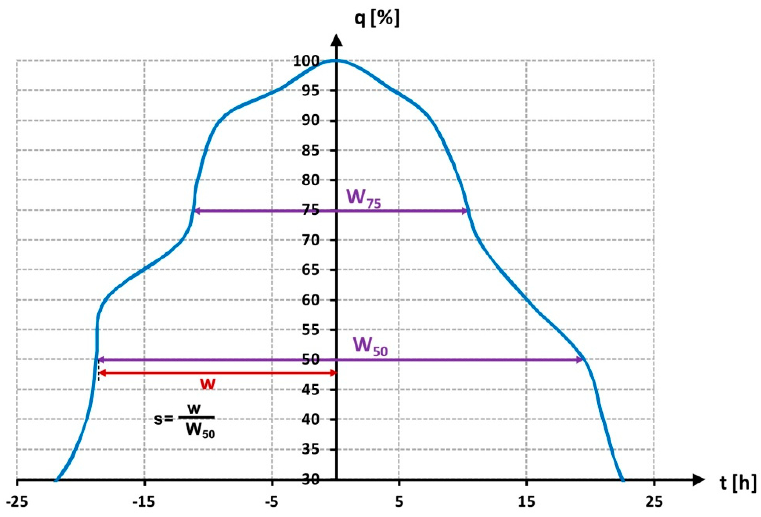
In the nonparametric approach, representative hydrographs characterize discharge changes in a standardized time scale. According to the method proposed by Archer et al. [1], DFH is developed as the median of annual maximum flow hydrographs observed in a given time period. It represents a kind of normalized flow hydrograph, where the flow values are expressed as a percentage p of the peak flow (q) between 0% and 100% along the width Wp of the hydrograph at a given percentage p of the peak flow (defined as the time during which the flow exceeds the value corresponding to the percentage of the peak discharge) [21,22,27]. The maximum of observed flow value corresponds to p = 100% and time t = 0; time for rising limb is expressed by negative values, and for a receding limb by positive values. Based on the nonparametric hydrograph, three parameters characterizing DFH (hydrograph descriptors) can be determined: W₅₀—hydrograph width at 50% of the peak flow (duration of exceedance of flow values for p = 50%); W₇₅—hydrograph width at 75% of the peak flow (duration of exceedance of flow values for p = 75%); and a skewness coefficient s, obtained by the ratio between the width component belonging to the rising limb and the total width (Figure 1). To obtain a robust form of nonparametric DFH, it is recommended to use data from a period of at least 30 years [27]. Moreover, the input, observed hydrographs used for DFH development, can be unimodal or multimodal [25,26]. Due to its empirical construction, the resulting DFH reflects specific catchment characteristics that impact flood wave formation, including physiographical, hydrological and climatological conditions.

2.2. Parametric DFH Estimation

Some of the first analytical descriptions of the hydrograph were the functions proposed by Reitz and Kreps [37], where a rising phase (0 ≤ t ≤ t_p) of a hydrograph was described as:

$$Q_t=Q_{max}·{\sin }^2\left(\frac{\mathsf{\pi }}{2}·\frac{t}{t_p}\right)$$

(1)

and a recession phase (t ≥ t_p) as:

$$Q_t=Q_{max}·{\exp }^{\left[-\propto \left(t-t_p\right)\right]}$$

(2)

where Q_t-flow at time t (m³s⁻¹); Q_max-maximum flow, usually the maximal annual flow with the assigned probability of exceedance (m³s⁻¹); t_p-time to peak (h); t-time counted from the assumed start of flood (h); $\propto$-coefficient, based on the shape of the observed hydrograph (h⁻¹).

A popular method developed in 1958 by Scarborough [38] was the parabolic curve method, which synthesized in two parts by parabolas passing through the peak flow at (0, 1) according to equations:

y = 1 + bx + cx²    for rising limb

(3)

y = 1 + Bx + Cx²    for receding limb

(4)

It is noteworthy that the parameters b, c, B, C can be related to the values of W₇₅, W₅₀ and s characterizing nonparametric DFH hydrograph developed according to the Archer method [39]:

$$q=1+\frac{2 W_{75}^2-W_{50}^2}{4 s W_{75} W_{50}\left(W_{75}-W_{50}\right)} t+\frac{2 W_{75}-W_{50}}{4 s^2 W_{75} W_{50 }(W_{75 }{W}_{50})} t^2$$

(5)

$$q=1+\frac{2 W_{75}^2-W_{50}^2}{4(1-s) W_{75} W_{50}\left(W_{75}-W_{50}\right)} t+\frac{2 W_{75}-W_{50}}{4 {(1-s)}^2 W_{75} W_{50 }(W_{75 }{W}_{50})} t^2$$

(6)

To obtain better results, further development of the parametric approach employing the Gamma distribution function was proposed by Nash [40]:

$$g=f\left(x\right)=\frac{1}{K\Gamma \left(n\right)} {\left(\frac{x}{K}\right)}^{n-1}\exp \left(-\frac{x}{K}\right)$$

(7)

where n-shape parameter; K-scale parameter; Γ(n)-the standard Gamma function.

The Gamma Function (7) has been further adopted by many authors [8,27,32,35,36] to represent the analytic expression of DFH:

$$q_t={\left(1+\frac{t}{t_p}\right)}^m\exp \left[-m \frac{t}{t_p}\right]100\%$$

(8)

for t ≥−t_p, where q_t-percent flow at time t, i.e., the percentage of peak flow at time t from the beginning of rising limb (%); t_p-time to peak (h); t-time from the beginning of rising limb (h); m-shape parameter (-).

Function (8) is found to be effective while describing the rising limb of the hydrograph, especially in the case of high flows (exceeding 50% of the maximum flow Q_max). In the lower part of the recession (falling) limb, large discrepancies are likely to occur. For this reason, in Ireland, the exponential function known as the UPO-ERR-Gamma (Unit-Peak-at-Origin Gamma curve coupled with an Exponential Replacement Recession curve) has been introduced to approximate the recession limb [8,27,41].

Strupczewski [35] proposed the use of the distribution function Pearson type III (currently referred to as the Gamma distribution) to describe a parametric hydrograph with two shape parameters, m and n [36,42,43].

$$q_t={\left(\frac{t}{t_p}\right)}^m\exp \left[\frac{m}{n}{\left(1-\frac{t}{t_p}\right)}^n\right]100\%$$

(9)

where q_t-percentile of the flow at the time t, counted from the beginning of the flood (%); t_p-time to peak (h); t-time from the assumed beginning of the flood (h); m, n-shape parameters (-).

In 1990, based on hydraulic analysis, Baptista introduced an analytic expression of design hydrograph based on the Gamma function with two parameters: shape parameter n, and a second parameter set to a constant value, m = 2 [33,34,44]:

$$q_t={\left(\frac{t}{t_p}\right)}^2\exp \left[\frac{2}{n}{\left(1-\frac{t}{t_p}\right)}^n\right]100\%$$

(10)

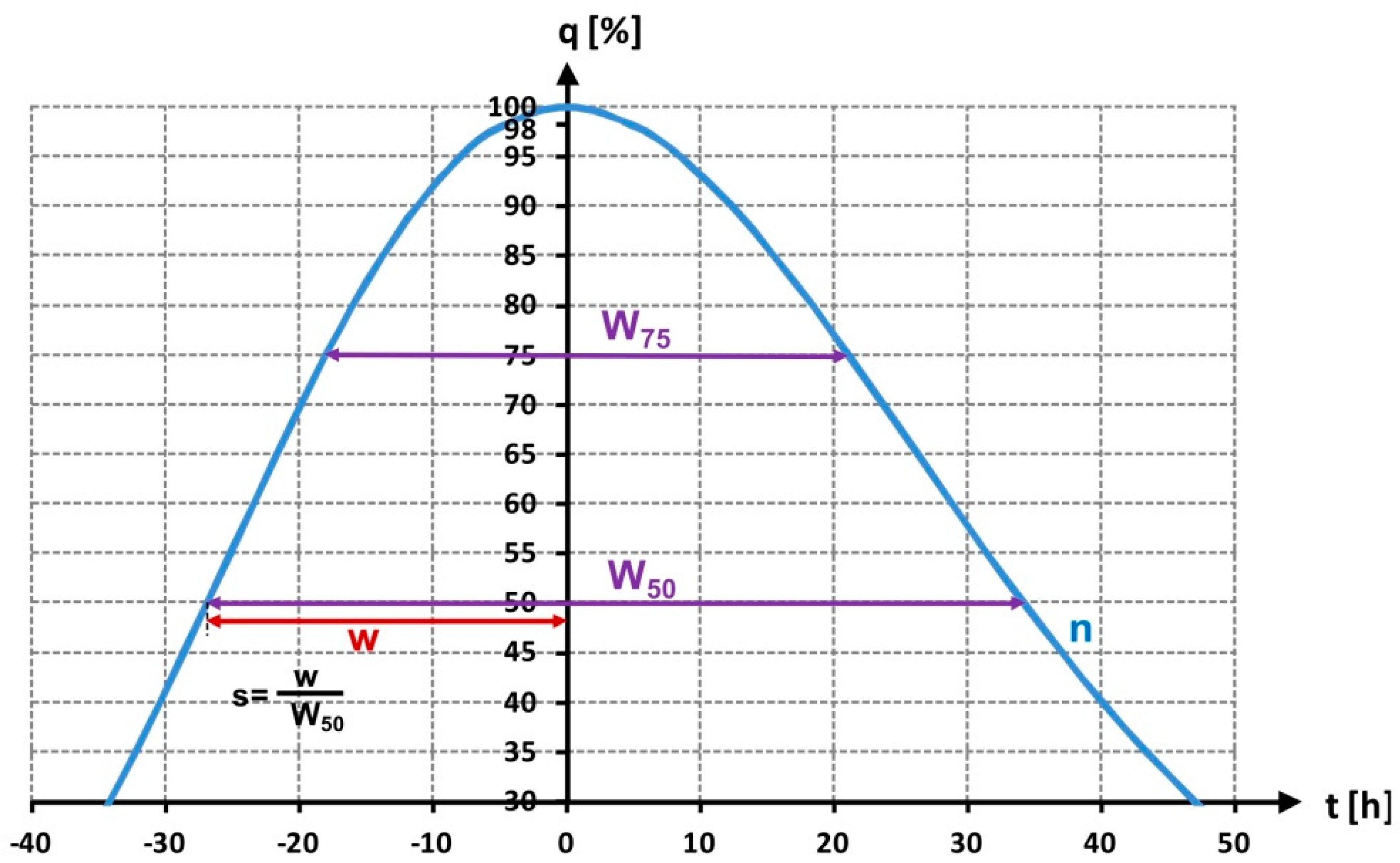
The main advantage of the parametric approach is the ability to estimate a flood hydrograph for any cross-section of the river by means of estimation of a small number of parameters [27,45,46]. In Figure 2, an exemplary parametric DFH is presented, along with the selected hydrograph descriptors (W₅₀, W₇₅ and s).

2.3. Hybrid Nonparametric and Parametric Approach

Our novel methodology proposed for DFH construction combines nonparametric and parametric approaches to benefit from both methods, while relating the parameters of the parametric DFH model with the catchment characteristics expressed through the selected properties of the nonparametric DFH model. The developed procedures include the following steps:

• Construction of nonparametric DFH using the Archer method based on long-term flow measurements for selected study catchments.
• Estimation of flood wave properties from developed nonparametric DFH: hydrograph width W₅₀ at percentage p = 50% of peak flow, W₇₅ at percentage p = 75% of the peak flow and a skewness coefficient s, representing catchment characteristics referred to as hydrograph descriptors.
• Based on the developed hydrograph descriptors (step b), estimation of the parameters of the parametric DFH.
• Validation of the correspondence between nonparametric DFH and parametric DFHs to recommend the parametric distribution model that best reproduces analyzed catchments’ flood wave properties.

In this study, three distributions, the original Gamma distribution (m, t_p), Gamma with modification by Strupczewski (m, n, t_p) and with modification by Baptista (n, t_p), were analyzed to recommend the PDF that best fits the assumed requirements: effectiveness in distribution parameter estimation and the best correspondence with the reference nonparametric DFH model developed with the use of the Archer method.

To estimate the parameters for each form of the Gamma distribution based on the hydrograph descriptors, the analytic expressions proposed by Strupczewski (9) and Baptista (10) were transformed to the following forms.

The adopted Strupczewski formula with two shape parameters, m and n:

$$q_t={\left(1+\frac{t}{t_p}\right)}^m\exp \left\{\frac{m}{n}\left[1-{\left(1+\frac{t}{t_p}\right)}^n\right]\right\}100\% \mathrm{for} t > –t_p$$

(11)

The adopted Baptista formula:

$$q_t={\left(1+\frac{t}{t_p}\right)}^2\exp \left\{\frac{2}{n}\left[1-{\left(1+\frac{t}{t_p}\right)}^n\right]\right\}100\% \mathrm{for} t > –t_p$$

(12)

For each form of Gamma distribution—(i) Formula (8), referred to as the Gamma method; (ii) Formula (11), referred to as the Strupczewski method; and (iii) Formula (12), referred to as the Baptista method—the corresponding distribution parameters, namely, shape parameters (m, n) and rising time (t_p), were estimated during the optimization process while minimizing S Function (13):

$$S={\left(W_{75}-\widehat{a}\right)}^2+{\left(b+\widehat{b}\right)}^2+{\left(c+\widehat{c}\right)}^2=\min$$

(13)

where W₇₅-duration of the exceedance of flow values for p = 75% of peak flow obtained from the nonparametric hydrograph (h); $\widehat{a}$-duration of the exceedance of flow values for p = 75% of peak flow estimated from one of the parametric formulas (Gamma, Strupczewski, Baptista) (h); b-duration of the exceedance of flow values for p = 50% of peak flow for the rising limb obtained from the nonparametric hydrograph, b = s·W₅₀ (h); $\widehat{b}$-duration of the exceedance of flow values for p = 50% of peak flow for the rising limb estimated from one of the parametric formulas (Gamma, Strupczewski, Baptista) (h); c-duration of the exceedance of flow values for p = 50% of peak flow for the receding limb obtained from the nonparametric hydrograph (h); $\widehat{c}$-duration of the exceedance of flow values for p = 50% of peak flow for the receding limb estimated from one of the parametric formulas (Gamma function, Strupczewski, Baptista) (h).

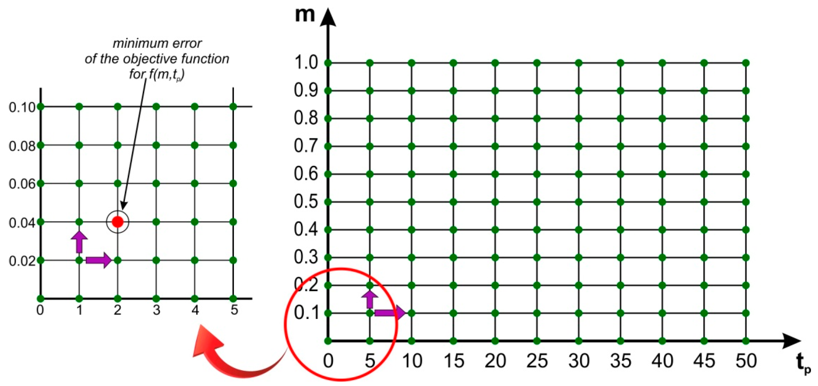
The optimalization procedure was performed with the use of the exhaustive search method, also known as the brute force method. According to this method, all possible combinations of discrete variables are examined to locate the optimal value. During this process, the values of the objective function for points that are equally distant from each other are compared. The search begins with the lower bound of the variable, and in a single iteration, the values of three consecutive points are compared using the assumption of unimodality [47,48]. The scheme of the method is shown in Figure 3. In the optimization procedure, the shape parameters m and n for the Strupczewski distribution method were assumed to be greater than 0. In all methods, the resolution of shape parameters adopted for calculations was 0.02, and 1 h for rising time t_p.

2.4. Study Area

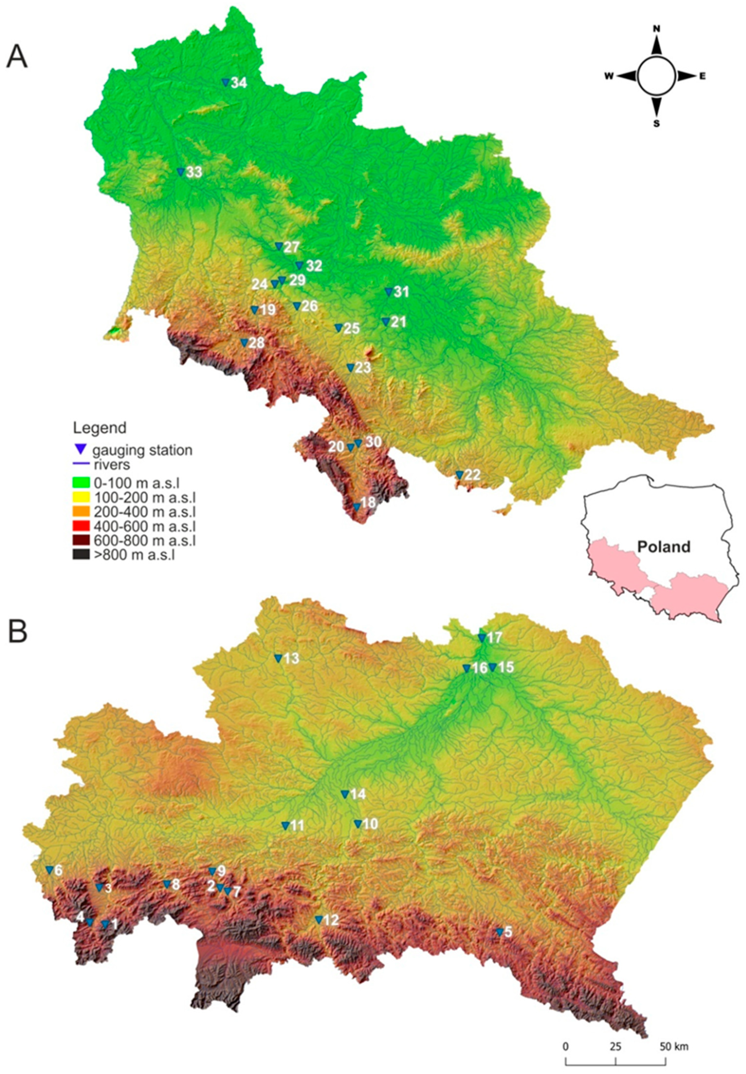
The study area is located in the south of Poland and includes 34 gauging stations: 17 located in the Upper Vistula River and 17 in the Middle Odra River water regions (Figure 4). The selected water regions represent areas of varying hydrographic characteristics as well as different geographic locations (mountains, upland and lowland). Analyzed catchments are also varying with respect to the catchment size, from close to 23 km² up to more than 50 thousand km² (see

Table 1. Values of hydrograph descriptors W₅₀, W₇₅ and s developed with the use of the Archer method.

No.	River	Gauging Station	Catchment Area (km2)	W50 (h)	W75 (h)	s (-)
Upper Vistula River water region
1	Żabniczanka	Żabnica	22.8	17.5	8.9	0.40
2	Lubieńka	Lubień	46.9	30.5	15.3	0.46
3	Żylica	Łodygowice	47.8	32.2	16.1	0.39
4	Bystra	Kamesznica	48.2	44.8	22.2	0.47
5	Wisłok	Puławy	131	24.3	10.4	0.47
6	Wisła	Skoczów	296	24.6	12.8	0.39
7	Raba	Kasinka Mała	353	20.5	10.2	0.43
8	Skawa	Sucha Beskidzka	468	26.5	13.2	0.49
9	Raba	Stróża	644	23.8	11.2	0.50
10	Biała	Koszyce Wielkie	957	18.6	9.3	0.47
11	Raba	Proszówki	1 470	44.6	21.6	0.51
12	Poprad	Stary Sącz	2 071	54.8	27.9	0.51
13	Nida	Brzegi	3 359	69.2	32.3	0.30
14	Dunajec	Żabno	6 735	57.2	27.9	0.58
15	San	Radomyśl	16 824	109.4	55.2	0.43
16	Wisła	Sandomierz	31 847	74.6	37.9	0.42
17	Wisła	Zawichost	50 732	143.8	48.4	0.29
Middle Odra River water region
18	Nysa Kłodzka	Międzylesie	49.7	9.1	3.9	0.45
19	Kaczawa	Świerzawa	133	17.9	8.6	0.38
20	Bystrzyca Dusznicka	Szalejów Dolny	175	10.1	3.7	0.37
21	Czarna Woda	Gniechowice	251	75.3	39.9	0.39
22	Biała Głuchołaska	Głuchołazy	283	15.9	6.4	0.29
23	Piława	Mościsko	292	68.1	34.5	0.33
24	Kaczawa	Rzymówka	314	28.0	15.5	0.31
25	Strzegomka	Łażany	362	57.8	38.0	0.28
26	Nysa Szalona	Jawor	304	25.9	13.5	0.43
27	Czarna Woda	Bukowna	431	167.1	100.2	0.20
28	Bóbr	Wojanów	535	38.2	15.7	0.19
29	Kaczawa	Dunino	774	32.8	14.2	0.32
30	Nysa Kłodzka	Kłodzko	1 084	15.1	6.85	0.47
31	Bystrzyca	Jarnołtów	1 721	77.5	36.3	0.24
32	Kaczawa	Piątnica	1 807	82.7	37.9	0.22
33	Bóbr	Żagań	4 255	114.8	45.2	0.25
34	Odra	Cigacice	39 900	250.4	109.8	0.37

).

The database used in the study consists of daily measurements recorded between 1964 and 2010 on the 34 selected water gauge stations.

3. Results

For each of the 34 analyzed water gauge stations, a series of annual maximum hydrographs was used to develop nonparametric DFHs according to the Archer method. The obtained values of the hydrograph descriptors W₅₀, W₇₅ and s are summarized in Table 1.

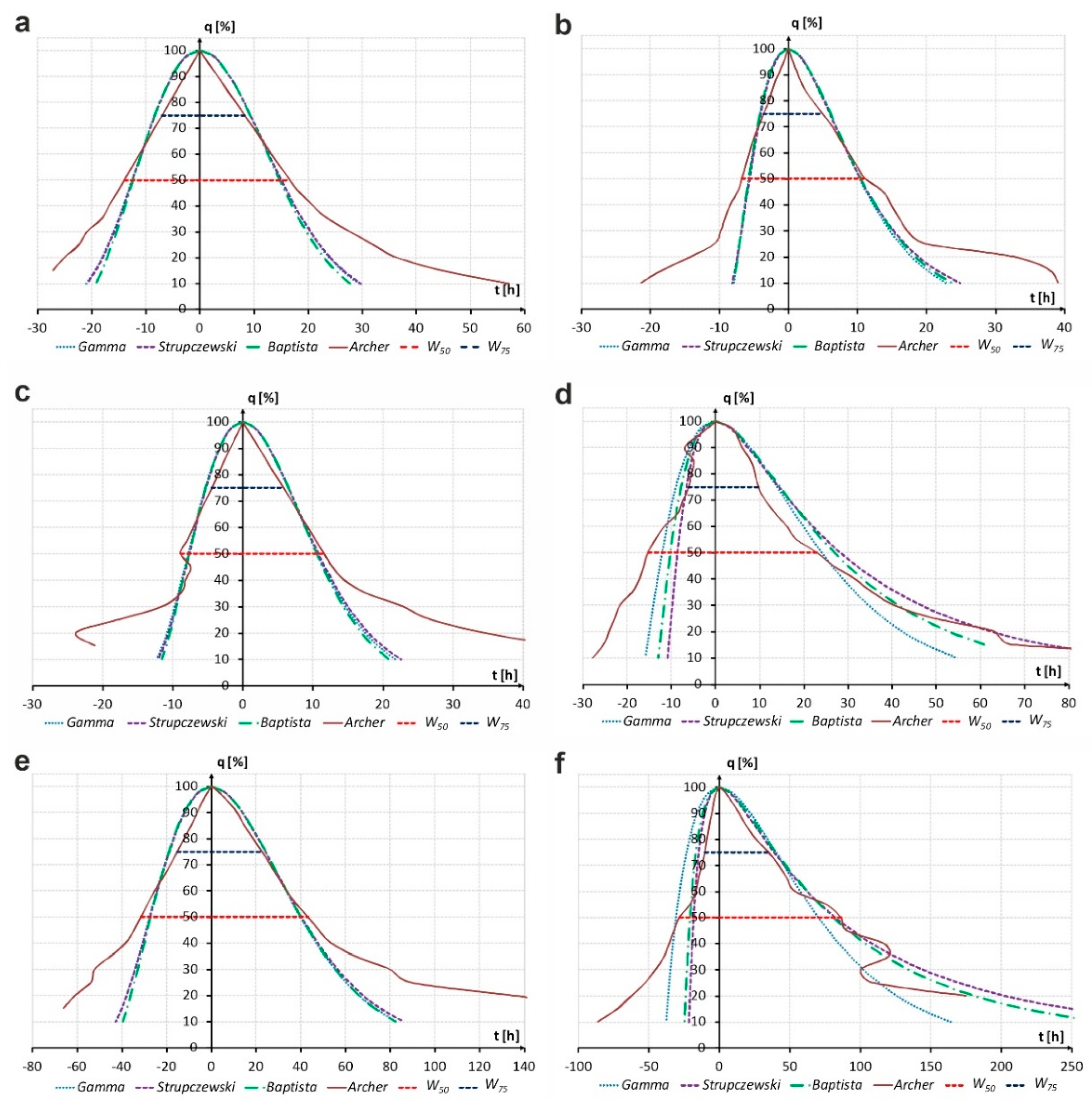
While minimizing the objective Function (13), the obtained values of the hydrograph descriptors were used to estimate the parameters of three parametric DFHs: Gamma (8), Strupczewski (11) and Baptista (12). The resulting distributions are presented in Figure 5, along with the reference nonparametric DFH model developed with the use of the Archer method. Due to the adopted criterions for the fitting procedure, better correspondence between parametric DFH and nonparametric DFH was obtained in the upper parts of the hydrographs above W₅₀. Values of the hydrograph descriptors (W₅₀, W₇₅ and s) estimated from fitted distributions are summarized in

Table 2. The values of parametric DFH characteristics W₅₀, W₇₅ and s estimated with the use of the analyzed methods: Gamma, Strupczewski and Baptista.

Water Gauge No.	Gamma			Strupczewski			Baptista
	W75	W50	s	W75	W50	s	W75	W50	s
1	10.2	16.0	0.39	10.1	16.0	0.39	10.2	16.0	0.38
2	17.7	27.5	0.45	17.7	27.5	0.45	17.6	27.0	0.45
3	18.5	29.1	0.37	18.4	29.2	0.37	18.4	28.9	0.36
4	25.8	40.1	0.47	25.8	40.1	0.46	25.9	39.8	0.47
5	13.2	20.5	0.44	13.3	20.6	0.46	13.3	20.4	0.47
6	14.5	22.7	0.38	14.2	22.6	0.37	14.4	22.5	0.38
7	11.8	18.4	0.42	11.8	18.4	0.41	11.8	18.2	0.42
8	15.3	23.7	0.47	15.3	23.8	0.49	15.3	23.8	0.49
9	13.4	20.8	0.46	13.5	20.9	0.50	13.5	20.7	0.51
10	10.7	16.7	0.45	10.8	16.7	0.47	10.7	16.5	0.46
11	25.5	39.5	0.48	25.5	39.6	0.51	25.6	39.3	0.51
12	31.9	49.5	0.48	32.0	49.6	0.51	32.0	49.2	0.52
13	38.2	61.5	0.27	36.8	62.6	0.26	36.5	62.4	0.24
14	41.0	63.7	0.48	32.4	51.4	0.60	32.4	51.0	0.60
15	63.3	98.7	0.42	63.2	99.0	0.42	63.7	98.3	0.41
16	43.3	67.5	0.41	43.2	67.8	0.41	43.4	67.2	0.41
17	70.1	116.8	0.20	64.8	119.5	0.20	65.6	117.4	0.21
18	4.9	7.8	0.44	4.9	7.8	0.44	4.9	7.6	0.43
19	10.2	16.1	0.36	10.0	16.1	0.35	10.3	16.3	0.35
20	5.4	8.5	0.36	4.9	8.1	0.30	5.4	8.5	0.36
21	44.4	69.5	0.38	44.1	69.9	0.37	44.2	69.0	0.38
22	9.0	14.2	0.37	8.6	14.2	0.30	9.2	14.4	0.38
23	39.0	62.1	0.30	38.2	62.9	0.30	38.8	63.2	0.30
24	16.7	26.7	0.28	16.2	26.9	0.30	15.9	26.5	0.27
25	38.1	60.4	0.32	34.7	57.9	0.28	37.3	60.8	0.30
26	15.1	23.6	0.42	15.1	23.7	0.42	15.2	23.4	0.42
27	107.3	171.2	0.29	97.0	170.6	0.22	96.2	172.2	0.21
28	22.9	36.2	0.33	20.9	36.8	0.23	22.3	37.1	0.27
29	18.1	28.6	0.34	17.1	28.7	0.28	17.5	29.2	0.27
30	8.3	13.0	0.44	8.4	13.0	0.46	8.4	12.9	0.47
31	46.2	73.4	0.31	39.5	72.2	0.20	41.9	71.7	0.24
32	49.3	78.3	0.31	41.4	77.6	0.18	43.7	78.3	0.21
33	63.5	101.0	0.30	53.5	100.5	0.18	56.8	101.8	0.21
34	134.1	212.8	0.31	134.3	217.7	0.33	134.2	215.7	0.32

.

In order to recommend the best parametric DFH model that reproduces the properties of the nonparametric DFH with the most accuracy, several quality measures recommended in the Technical Research Report Volume III Hydrograph Analysis [27] were applied to assess the agreement between the parametric and nonparametric hydrographs: relative error (RE) and mean relative error (MRE) of the hydrograph width. Other measures applied for parametric versus the reference nonparametric DFH model assessment were statistical measures: correlation coefficient (r), root mean square error (RMSE) and mean absolute error (MAE). To evaluate the correspondence of flood wave shape and volume, the values of volumes of hydrographs and the hydrograph’s center of gravity for the time coordinate obtained with the proposed and reference methods were compared.

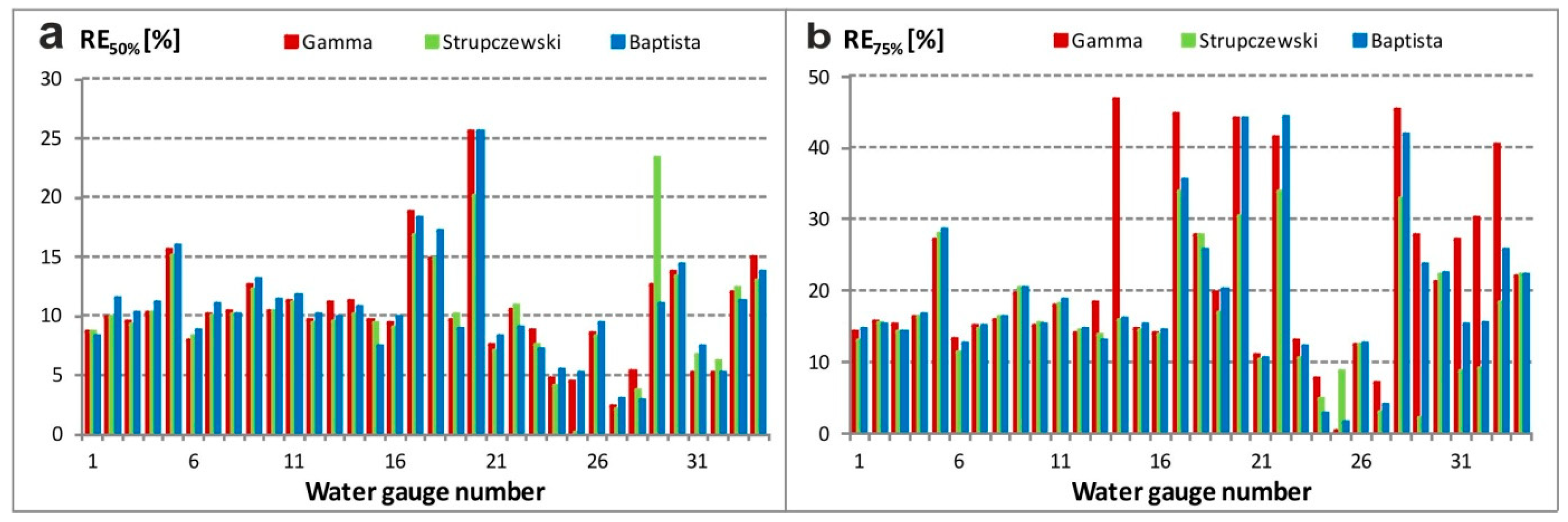
Relative error of hydrograph width was calculated according to the following formula:

$$R{E}_p=\frac{\left|W_p-\widehat{W_p}\right|}{W_p}$$

(14)

where RE_p-relative error of hydrograph width W_p, p = 50%, p = 75%; W_p-hydrograph width at p = 50%, p = 75%, estimated from the nonparametric design hydrograph (h); $\widehat{W_p}$-hydrograph width at p = 50%, p = 75%, estimated from the parametric hydrograph according to applied formulas in the respective methods (Gamma, Strupczewski, Baptista) (h).

Figure 6 presents a comparison of RE_50% and RE_75% calculated for hydrograph width at the level of W₅₀ and W₇₅, respectively, for each water gauge station. In the estimation of time of duration of flow values above 50% of peak flow, the RE values were mostly at the level of 10%. Estimation of time of duration of flow values above 75% of peak flow in most of the cases provided correspondence between this attribute of DFH from parametric and nonparametric methods not exceeding 20%; however, for the Gamma model, 6 of 34 water gauge stations RE_75% exceeded 40%.

Based on the values of RE calculated at different levels of percent of the peak flow, mean relative error [49] was estimated to assess the compliance of the parametric and nonparametric hydrographs according to the following definition:

$$MR{E}_p= \frac{1}{N_p}{\displaystyle \sum }_{i=1}^{N_p}R{E}_i$$

(15)

where $MR{E}_p$-mean relative error for the p-percent of the peak flow (i.e., p = 75% and p = 50%); N_p-number of assumed levels of percent of the peak flow (i.e., N_p = 6 for p = 75% and N_p = 11 for p = 50% for percent levels i: p₁ = 98, p₂ = 95, p₃ = 90, p₄ = 85, p₅ = 80, p₆ = 75,…, p₁₁ = 50, RE_i-relative error for each percent level.

For the set of analyzed water gauges, MRE was calculated for the hydrograph truncated at the level of p = 50% and at the level p = 75% (Figure 7). The obtained results indicate the worst performance of the Gamma distribution compared to Strupczewski and Baptista methods. MRE₅₀ values not exceeding a level of 30 were found in 12 cases for the Strupczewski distribution, and in 10 for the Baptista and Gamma models. MRE₇₅ values not exceeding a level of 60 were found in 18 cases for Strupczewski, in 16 for the Baptista method and only in 13 for Gamma distribution. However, still, the quality measures recommended by O’Connor [27] did not assure explicit recommendation for the Vistula or the Oder water region applications. Similar ambiguity in MRE results’ interpretation was reported by Chai and Draxler [50].

Correlation coefficient (r), root mean square error (RMSE) and mean absolute error (MAE) were calculated according to the following definitions:

$$r=\frac{{{\displaystyle \sum }}_{i=1}^n\left(x_i-\overline{x}\right)\left(y_i-\overline{y}\right)}{\sqrt{{{\displaystyle \sum }}_{i=1}^n{\left(x_i-\overline{x}\right)}^2}\sqrt{{{\displaystyle \sum }}_{i=1}^n{\left(y_i-\overline{y}\right)}^2}}$$

(16)

$$RMSE=\sqrt{\frac{1}{n}{{\displaystyle \sum }}_{i=1}^n{\left(x_i-y_i\right)}^2}$$

(17)

$$MAE=\frac{{{\displaystyle \sum }}_{i=1}^n\left|y_i-x_i\right|}{n}$$

(18)

where x_i-value of descriptor: W₅₀ or W₇₅ or s estimated from the analyzed parametric DFH models (Gamma, Strupczewski, Baptista); y_i-value of descriptor: W₅₀ or W₇₅ or s from nonparametric reference DFH; $\overline{x}$-mean value of descriptor: W₅₀ or W₇₅ or s estimated from the analyzed parametric DFH models (Gamma, Strupczewski, Baptista); $\overline{y}$-mean value of descriptor: W₅₀ or W₇₅ or s from nonparametric reference DFH; n—sample size.

The r, RMSE and MAE statistics also acknowledged the better fit of the Baptista and Strupczewski distributions than the commonly used Gamma distribution in terms of agreement between the analyzed hydrograph descriptors (W_50, W₇₅ and s) and their reference values. This advantage was particularly evident for the skewness coefficient s in the middle Odra River water region (see

Table 3. The values of statistical measures: correlation coefficient (r), root mean square error (RMSE) and mean absolute error (MAE) for DFH characteristics W₅₀, W₇₅ and s estimated with the use of the analyzed methods, Gamma, Strupczewski and Baptista, for the upper Vistula River water region, middle Odra River water region and both water regions.

	Gamma			Strupczewski			Baptista
Type of Statistic	W75	W50	s	W75	W50	s	W75	W50	s
Upper Vistula River water region
r	1.00	0.97	0.98	1.00	0.99	0.99	1.00	0.98	0.98
RMSE	8.8	7.0	0.1	7.5	5.3	0.0	7.6	6.7	0.0
MAE	6.6	4.0	0.1	5.4	4.0	0.0	5.7	4.4	0.0
Middle Odra River water region
r	1.00	0.99	0.81	1.00	0.99	0.88	0.99	0.99	0.98
RMSE	12.1	8.1	0.1	9.2	6.8	0.0	9.6	7.6	0.0
MAE	7.1	5.4	0.1	5.2	4.2	0.0	5.7	4.9	0.0
The whole area
r	1.00	0.99	0.82	1.00	0.99	0.95	0.99	0.98	0.98
RMSE	10.6	7.5	0.1	8.4	6.1	0.0	8.7	7.2	0.0
MAE	6.8	4.7	0.1	5.3	4.1	0.0	5.7	4.7	0.0

).

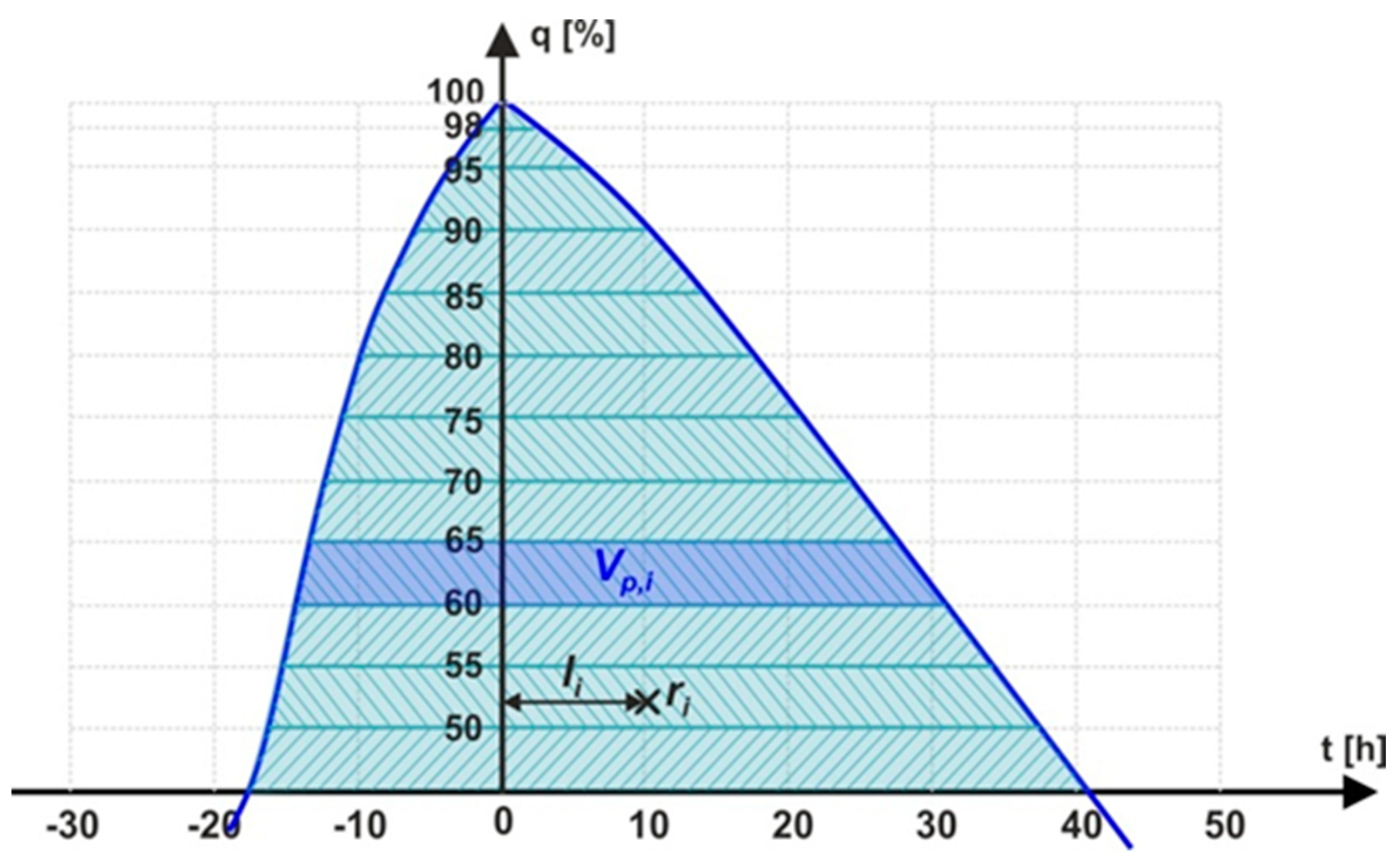
The volume of the hydrograph truncated at the level of p-percent of the peak flow was calculated according to the following formula (see Figure 8):

$$V_p={{\displaystyle \sum }}_{i=1}^{N_p}{V}_{p,i }$$

(19)

where V_p-the volume of the hydrograph above the p-percent of the peak flow, p = 50%, p = 75%; N_p-number of assumed levels of percent of the peak flow (N_50% = 11 for p = 50% and N_75% = 6 for p = 75%); V_p,i-partial volume of the hydrograph between successive levels of percent of the peak flow (Figure 8).

The center of gravity for the time coordinate was calculated for the hydrograph truncated at the level of p-percent of the peak flow according to the following formula:

$$r_p=\frac{{{\displaystyle \sum }}_i^{N_p}{V}_{p,i }{l}_i}{{{\displaystyle \sum }}_i^{N_p}{V}_{p,i }}$$

(20)

where r_p-time coordinate of the center of gravity of the hydrograph truncated at the level of p-percent of the peak flow (h); N_p-number of assumed levels of percent of the peak flow number of percent flows exceeding p-percent flow (N_50% = 11 for p = 50% and N_75% = 6 for p = 75% and 11 for p = 50%); V_p,i-partial volume of the hydrograph between successive levels of p-percent of the peak flow (h); l_i-time coordinate for the gravity center r_i of the partial volume (h) (see Figure 8); r_i-the gravity center of the partial volume.

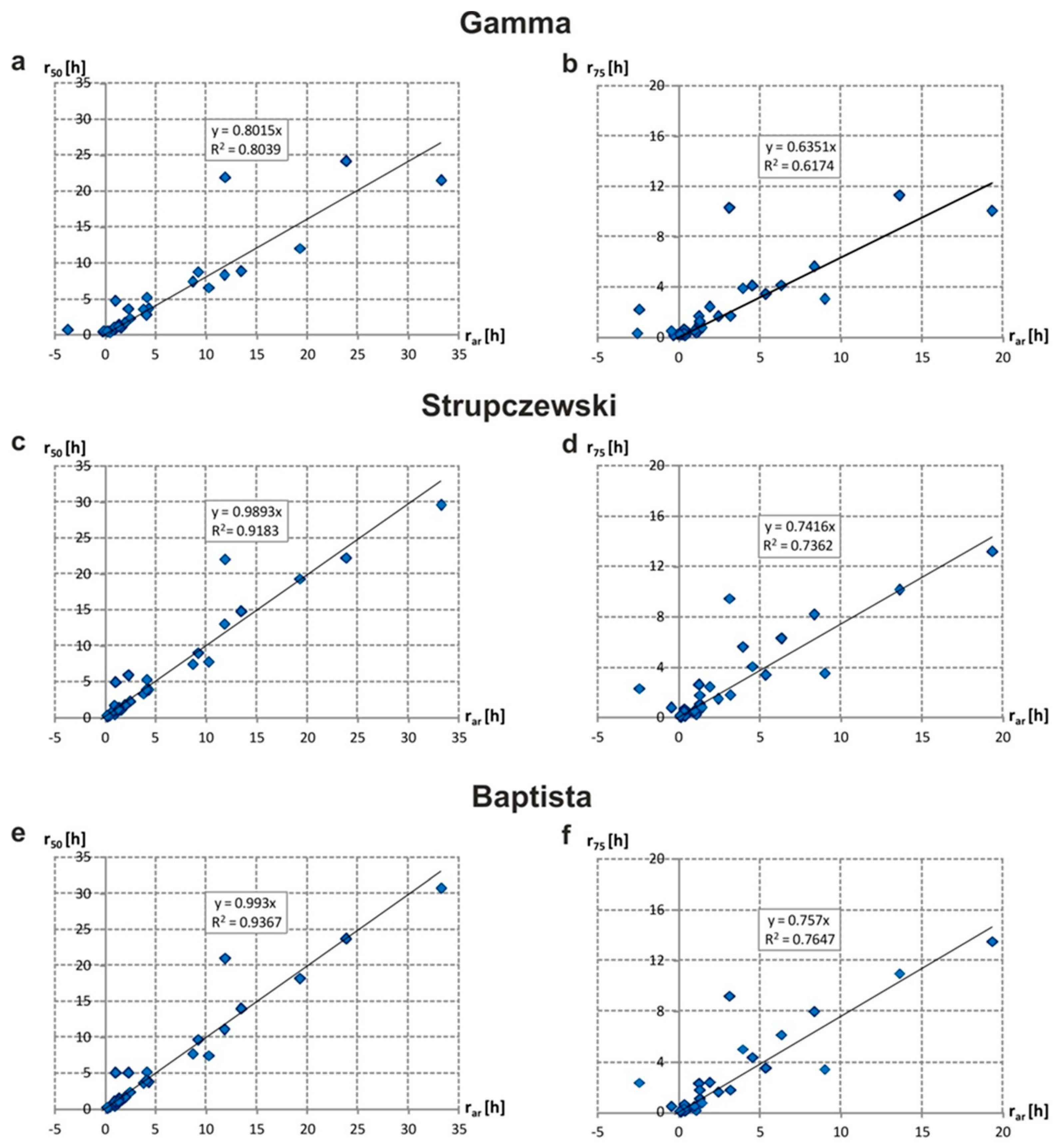
Figure 9 shows correlation plots between the values of the gravity centers estimated from the parametric hydrograph versus nonparametric hydrograph developed with the Archer method (r_ar) for W₅₀ (r_50%) and W₇₅ (r_75%). The obtained results indicate that Strupczewski and Baptista distribution methods provided a very good fit, outperforming Gamma distribution at both truncation levels, p = 50% and p = 75%. The coefficient of determination R² was 0.937 for W₅₀ and 0.765 for W₇₅ in the Baptista model, while for the Gamma distribution, R² was 0.804 for W₅₀ and 0.617 for W₅₀.

The comparison of volumes obtained from parametric hydrographs with nonparametric hydrographs shows the high compliance (R² exceeding 0.99 for level of truncations p = 50% and 0.96 for p = 75%) in all three distribution methods (Figure 10).

The obtained values of the applied quality assessment measures advocate for the selection of the Strupczewski or Baptista method for parametric DFH development in the Oder and Vistula water regions according to the proposed hybrid approach.

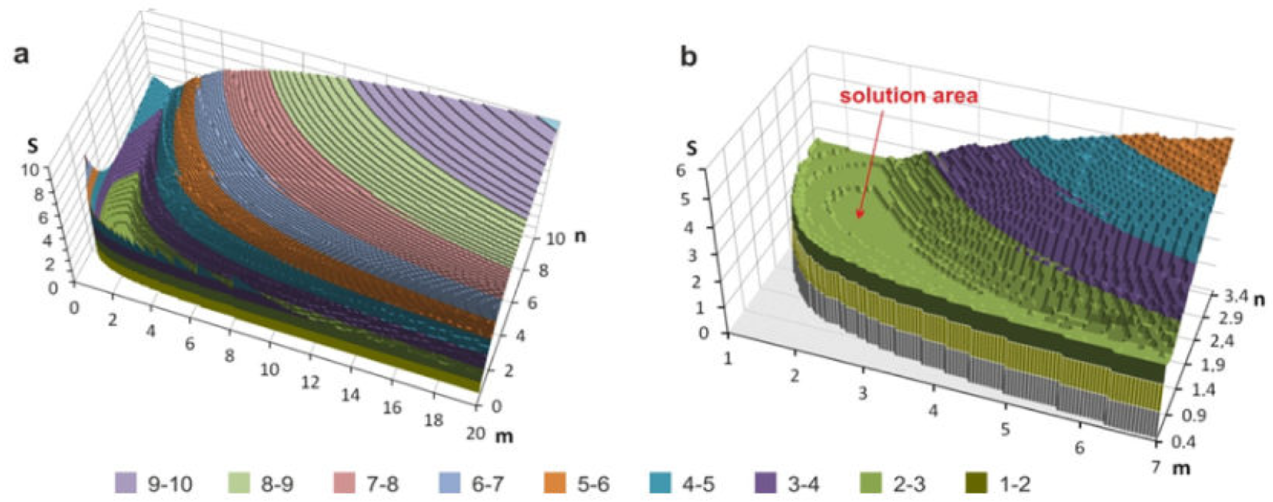
Since the Strupczewski formula employs two shape parameters, m and n [51], it was anticipated that this distribution method could provide the best results. Tests carried out for the Pearson type IV distribution with two shape parameters have shown that several pairs of parameters m and n minimize the objective function [52]. A similar test was carried out for the distribution function proposed by Strupczewski with the applied objective Function (13). The area of solutions meeting the adopted criteria proves that there is an equifinality problem; that is, many pairs of the distribution parameters values m and n return substantially the same result (Figure 11). Therefore, the Strupczewski distribution method was ultimately not recommended to be used for parametric hydrograph estimation according to the proposed methodology and applied objective function.

4. Conclusions and Discussion

Greater flood damage is associated with a larger budget required for flood protection. To prepare for major disasters, governments should allocate enough organizational, financial and technical resources according to the damages that occurred and the risks assessed. Investing in disaster risk reduction is fundamental for achieving the Sustainable Development Goals since natural hazards can impede sustainable development by causing economic and human losses [53]. Proper understanding of flood risks is not easy for policy makers or for ordinary residents [54]. It is crucial to identify the areas that are particularly threatened by flooding. Flood hazard maps that visualize the areas that are inundated by floodwater of various return periods constitute a critical instrument in the decision-making process. In Poland, flood hazard maps were developed for the majority of catchments, mainly the ones controlled with water gauge stations to provide local authorities information on flood hazard zones. For their construction, hydraulic two-dimensional models were used to forecast the water flow surface during the flood wave. This requires information on flood wave volume, shape and maximum flow. For the gauged river sections, flood hydrographs were obtained from observations through nonparametric statistical methods. The problem is progressing in the case of ungauged cross-sections. The common procedure is to apply rainfall–runoff models. Their shortcomings are the lack of recommended rainfall hyetographs, high sensitivity of synthetic UH to the distribution of rainfall gauge stations, errors in rain data and delineation of precipitation spatial distribution. These setbacks cost time and resources and induce the development of DFH with the use of statistical parametric methods.

The objective of this work was to introduce a hybrid approach for DFH development that employs nonparametric and parametric methods. The idea behind the concept was the estimation of the parametric DFH with the set of limited catchment characteristics developed from observations in a systematized method of nonparametric DFH construction according to the Archer method. In the presented approach, catchment characteristics are summarized with three hydrograph descriptors (duration of exceedance of flow values corresponding to 50% and 75% of peak flow, as well as the hydrograph skewness descriptor s) attributing to the upper part of the median hydrograph. This compilation of both methods involves the identification of the parametric method that provides the best fit to the reference nonparametric DFH model. The analyzed candidates for parametric distributions models were the Gamma distribution with one shape parameter, m; the Strupczewski distribution with two shape parameters, m and n; and the Baptista method with two shape parameters, n and a constant parameter m = 2.

The assessment of the quality of correspondence between the considered parametric models to the reference nonparametric hydrographs was based on relative error (RE) and mean relative error (MRE), supported with the assessment of the hydrograph center of gravity and hydrograph volume truncated at selected probability levels (50% and 75%). Additionally, the quality of model fit was analyzed using the statistical measures r, RMSE and MAE. According to the results obtained, the Gamma distribution gave the worst performance in the analyzed study area. This conclusion was confirmed with the results of the assessment of the centers of gravity and hydrograph volumes. For the Strupczewski distribution model, many potential hydrograph parameters m and n pairs that met the assumed optimization criterion were found, resulting in difficulties in the determination of the parametric form of the hydrograph. Therefore, within the framework of the developed approach, the recommendation of the authors is to apply the Baptista model as the parametric DFH model for the Vistuala and the Odra water region.

The estimation of the parametric model parameters based on a limited number of descriptors W₇₅, W₅₀ and s allows us to construct the hydrograph of a flood peak of given return period at gauged and ungauged sites. At gauged sites, hydrograph width descriptors are estimated from the analysis of observed flood hydrographs. At ungauged sites, a regression-based estimate relating sought DFH properties with physical catchment descriptors [45] can be applied [26]. This is a major advantage of the proposed hybrid approach, since a parametric hydrograph can be developed for any river cross-section. The proposed approach aims to constitute an universal approach that could be valid for various applications that environmental protection is tackling, starting from flood hazard map development.

To deepen the understanding of flood formation and the perdition of flood zones, future method development is directed towards the implementation of new technologies of Earth observation, with emphasis on remote sensing (RS). Satellite-based Earth observation techniques can be used for preparing near real-time flood maps and assessing damage to residential properties, infrastructure and crops. Flood maps provide essential inputs for assessing the progression of the inundation area and the severity of the flood. Optical remote sensing and SAR data are more sensitive to water bodies and are helpful for determining flood frequency and severity and achieving accurate measurements of streams, lakes and wetlands [55]. Employing RS supported with machine learning (ML) algorithms provides an innovative method for the detection of real flood-affected areas [56]. This information can be applied as a reference for the validation of different DFH models introduced to hydrodynamical models to achieve a new quality of flood hazard mapping and managing flood risks.

The other examples that require efficient methods for flood wave estimation include designing hydraulic structures and reservoirs to mitigate the effects of floods and droughts [57,58], dam safety assessment and predicting the hydrologic effects of different water and land use management scenarios. The knowledge of flood wave properties and transformation in a riverbed is also crucial for designing objects in urbanized catchments, where rainwater is introduced to the sewer systems and where the level of surface runoff plays a key role in flood risk estimation [59,60,61]. Moreover, climate change exacerbates the impact of extreme phenomena such as flash floods, for which the evaluation of flood wave characteristics has become critical [62,63,64,65].

References

- Shreevastav, B.B.; Tiwari, K.R.; Mandal, R.A.; Nepal, A. Assessing Flood Vulnerability on Livelihood of the Local Community: A Case from Southern Bagmati Corridor of Nepal. Prog. Disaster Sci. 2021, 12, 100199. [Google Scholar] [CrossRef]
- Vrijling, J.K.; van Hengel, W.; Houben, R.J. Acceptable Risk as a Basis for Design. Reliab. Eng. Syst. Saf. 1998, 59, 141–150. [Google Scholar] [CrossRef]
- Apel, H.; Thieken, A.H.; Merz, B.; Blöschl, G. A Probabilistic Modelling System for Assessing Flood Risks. Nat. Hazards 2006, 38, 79–100. [Google Scholar] [CrossRef]
- Criss, R.E.; Winston, W.E. Properties of a Diffusive Hydrograph and the Interpretation of Its Single Parameter. Math. Geosci. 2008, 40, 313–325. [Google Scholar] [CrossRef]
- Serinaldi, F.; Grimaldi, S. Synthetic Design Hydrographs Based on Distribution Functions with Finite Support. J. Hydrol. Eng. 2011, 16, 434–446. [Google Scholar] [CrossRef]
- Hattermann, F.F.; Kundzewicz, Z.W.; Huang, S.; Vetter, T.; Gerstengarbe, F.-W.; Werner, P. Climatological Drivers of Changes in Flood Hazard in Germany. Acta Geophys. 2013, 61, 463–477. [Google Scholar] [CrossRef]
- Alfieri, L.; Feyen, L.; Salamon, P.; Thielen, J.; Bianchi, A.; Dottori, F.; Burek, P. Modelling the Socio-Economic Impact of River Floods in Europe. Nat. Hazards Earth Syst. Sci. 2016, 16, 1401–1411. [Google Scholar] [CrossRef] [Green Version]
- Goswami, M. Generating Design Flood Hydrographs by Parameterizing the Characteristic Flood Hydrograph at a Site Using Only Flow Data. Hydrol. Sci. J. 2020, 1–19. [Google Scholar] [CrossRef]
- Jain, S.K. Engineering Hydrology: An Introduction to Processes, Analysis, and Modeling; McGraw-Hill Education: New York, NY, USA, 2019; ISBN 978-1-259-64197-8. [Google Scholar]
- Snyder, F.F. Synthetic Unit-Graphs. Trans. AGU 1938, 19, 447. [Google Scholar] [CrossRef]
- Chow, V.T.; Maidment, D.R.; Mays, L.W. Applied Hydrology, international ed.; McGraw-Hill series in water resources and environmental engineering; McGraw-Hill: New York, NY, USA, 1988; ISBN 978-0-07-100174-8. [Google Scholar]
- USDA Hydrographs, Part 630, Hydrology, Hydraulics and Hydrology-Technical References NRCS National Engineering Handbook; U.S. Department of Agriculture: Washington, DC, USA, 2007.
- Garrett, R.C.; Woolverton, A.H. The Unit Hydrograph-Its Construction and Uses; Texas State Board of Water Engineers: Austin, TX, USA, 1951. [Google Scholar]
- Ozga-Zielińska, M.; Gądek, W.; Książyński, K.; Nachlik, E. Mathematical Model of Rainfall-Runoff Transformation-WISTOO. In Mathematical Models of Large Watershed Hydrology; Singh, V.P., Frevert, D.K., Eds.; Water Resources Publications: Highlands Ranch, CO, USA, 2002; pp. 811–860. ISBN 978-1-887201-34-6. [Google Scholar]
- Wałęga, A. Application of HEC-HMS Programme for the Reconstruction of a Flood Event in an Uncontrolled Basin/Zastosowanie Programu HEC-HMS Do Odtworzenia Wezbrania Powodziowego w Zlewni Niekontrolowanej. J. Water Land Dev. 2013, 18, 13–20. [Google Scholar] [CrossRef]
- Pietrusiewicz, I.; Cupak, A.; Wałęga, A.; Michalec, B. The Use of NRCS Synthetic Unit Hydrograph and Wackermann Conceptual Model in the Simulation of a Flood Wave in an Uncontrolled Catchment/Zastosowanie Syntetycznego Hydrogramu Jednostkowego NRCS Oraz Konceptualnego Modelu Wackermana Do Symulacji Fali Wezbraniowej w Zlewni Niekontrolowanej. J. Water Land Dev. 2014, 23, 53–59. [Google Scholar] [CrossRef] [Green Version]
- Gądek, W.; Bodziony, M. The Hydrological Model and Formula for Determining the Hypothetical Flood Wave Volume in Non-Gauged Basin. Meteorol. Hydrol. Water Manag. 2015, 3, 3–10. [Google Scholar] [CrossRef] [Green Version]
- Methods of Hydrological Computations for Water Projects: A Contribution to the International Hydrological Programme: Report; Eichert, B. (Ed.) Studies and reports in hydrology; Unesco: Paris, France, 1982; ISBN 978-92-3-102005-6. [Google Scholar]
- Archer, D.; Foster, M.; Faulkner, D.; Mawdsley, J. The Synthesis of Design Flood Hydrographs; All Jeremy Benn Associates, Gillow House, Broughton Hall, Skipton: New York, NY, USA, 2000. [Google Scholar]
- Sauquet, E.; Ramos, M.-H.; Chapel, L.; Bernardara, P. Streamflow Scaling Properties: Investigating Characteristic Scales from Different Statistical Approaches. Hydrol. Processes 2008, 22, 3462–3475. [Google Scholar] [CrossRef]
- Gądek, W.; Baziak, B.; Tokarczyk, T. Nonparametric Design Hydrograph in the Gauged Cross Sections of the Vistula and Odra Basin. Meteorol. Hydrol. Water Manag. 2017, 5, 53–61. [Google Scholar] [CrossRef] [Green Version]
- Gądek, W.; Baziak, B.; Tokarczyk, T. Strupczewski Method for Parametric Design Hydrographs in Ungauged Cross-Sections. Arch. Hydro-Eng. Environ. Mech. 2017, 64, 49–67. [Google Scholar] [CrossRef] [Green Version]
- Merleau, J.; Perreault, L.; Angers, J.-F.; Favre, A.-C. Bayesian Modeling of Hydrographs. Water Resour. Res. 2007, 43. [Google Scholar] [CrossRef] [Green Version]
- Yue, S.; Ouarda, T.B.M.J.; Bobée, B.; Legendre, P.; Bruneau, P. Approach for Describing Statistical Properties of Flood Hydrograph. J. Hydrol. Eng. 2002, 7, 147–153. [Google Scholar] [CrossRef]
- Gądek, W.; Środula, A. The Evaluation of the Design Flood Hydrographs Determined with the Hydroproject Method in the Gauged Catchments. Infrastrukt. Ekol. Teren. Wiej./Infrastruct. Ecol. Rural. Areas 2014, IV/3, 1355–1366. [Google Scholar] [CrossRef]
- Gądek, W.; Tokarczyk, T. Determining Hypothetical Floods in the Odra Basin by Means of the Cracow Method and the Volume Formula. Infrastrukt. Ekol. Teren. Wiej. 2015, 1507–1519. [Google Scholar] [CrossRef]
- O’Connor, K.; Goswami, M.; Faulkner, D. Flood Studies Update Technical Research Report-Volume III-Hydrograph Analysis; NUI Galway and JBA Consulting, Office of Public Work: Dublin, Ireland, 2014.
- Qamar, M.U. Parametric and Non-Parametric Approaches for Runoff and Rainfall Regionalization. Ph.D. Thesis, Polytechnic University of Turin, Turin, Italy, 2015. [Google Scholar] [CrossRef]
- Brunner, M.I.; Viviroli, D.; Sikorska, A.E.; Vannier, O.; Favre, A.; Seibert, J. Flood Type Specific Construction of Synthetic Design Hydrographs. Water Resour. Res. 2017, 53, 1390–1406. [Google Scholar] [CrossRef] [Green Version]
- Debele, S.E.; Strupczewski, W.G.; Bogdanowicz, E. A Comparison of Three Approaches to Non-Stationary Flood Frequency Analysis. Acta Geophys. 2017, 65, 863–883. [Google Scholar] [CrossRef]
- Aranda, J.; García-Bartual, R. Synthetic Hydrographs Generation Downstream of a River Junction Using a Copula Approach for Hydrological Risk Assessment in Large Dams. Water 2018, 10, 1570. [Google Scholar] [CrossRef] [Green Version]
- McEnroe, B.M. Preliminary Sizing of Detention Reservoirs to Reduce Peak Discharges. J. Hydraul. Eng. 1992, 118, 1540–1549. [Google Scholar] [CrossRef]
- Baptista, M.; Michel, C. Influence des caracteristiques hydrauliques des bies sur la propagation des pointes de crue. La Houille Blanche 1990, 2, 141–148. [Google Scholar] [CrossRef] [Green Version]
- Baptista, M. Contribution à L’étude de la Propagation de Crues en Hydrologie; Ecole Nationale des Ponts et Chaussées, CEMAGREF Antony Cedex. 1990. Available online: https://pastel.archives-ouvertes.fr/pastel-00568722/document (accessed on 1 June 2022).
- Strupczewski, W.G. Equation of Flood Crest. Wiadomości Służby Hydrologicznej i Meteorologicznej 1964, 2, 35–58. [Google Scholar]
- Strupczewski, W.G.; Bogdanowicz, E.; Kochanek, K. Discussion of “Synthetic Design Hydrographs Based on Distribution Functions with Finite Support” by Francesco Serinaldi and Salvatore Grimaldi. J. Hydrol. Eng. 2013, 18, 121–126. [Google Scholar] [CrossRef]
- Reitz, W.; Kreps, H. Näherungsverfahren zur Berechnung des Erforderlichen Struraumes für Zwecke des Hochwasserschutzes; Deutsche Wasserwirtschaft: Hennef, Germany, 1945; Volume 1. [Google Scholar]
- Scarborough, J.B. Numerical Mathematical Analysis; Johns Hopkins Press: Baltimore, MD, USA, 1958. [Google Scholar]
- Reed, D.W.; Marshall, D.C. Defining a Design Hydrograph. In Flood Estimation Handbook; Institute of Hydrology, Centre for Ecology and Hydrology: Wallingford, UK, 1999; ISBN 978-1-906698-01-0. [Google Scholar]
- Nash, J.E. The Form of the Instantaneous Unit Hydrograph. In Proceedings of the International Association of Hydrological Sciences General Assembly, Toronto, ON, Canada; 1957; Volume 3, pp. 114–121. Available online: https://nora.nerc.ac.uk/id/eprint/508550/ (accessed on 1 June 2022).
- Reddyvaraprasad, C.; Patnaik, S.; Biswal, B. Recession Flow Prediction in Gauged and Ungauged Basins by Just Considering Past Discharge Information. Hydrol. Sci. J. 2020, 65, 21–32. [Google Scholar] [CrossRef]
- Cieplowski, A. Statistical Methods of Determining Typical Winter and Summer Hydrographs for Ungauged Watersheds; Louisiana State University: Baton Rouge, LA, USA, 1987; pp. 117–124. [Google Scholar]
- Cieplowski, A. Relationships between Selected Elements of the Flood Hydrographs in Rivers. J. Water Land Dev. 2001, 5, 89–105. [Google Scholar]
- Gądek, W.; Baziak, B.; Tokarczyk, T.; Bodziony, M. Flow Descriptors for Parametric Hydrographs Accounting for Afforestation of the Catchment. Meteorol. Hydrol. Water Manag. 2019, 36–45. [Google Scholar] [CrossRef]
- Bayliss, A.C. Catchment Descriptors Volume in Flood Estimation Handbook/Institute of Hydrology; Centre for Ecology and Hydrology: Wallingford, UK, 1999; ISBN 978-1-906698-01-0. [Google Scholar]
- Mills, P.; Nicholson, O.; Reed, D.W. Flood Studies Update Technical Research Report-Volume IV-Physical Catchment Descriptors; NUI Galway and JBA Consulting, Office of Public Work, 2014. Available online: https://data.gov.ie/dataset/flood-studies-update-fsu-physical-catchment-descriptors-ungauged (accessed on 1 June 2022).
- Deb, K. Optimization for Engineering Design: Algorithms and Examples; PHI Learning Private Limited: New Delhi, India, 2016; ISBN 978-81-203-4678-9. [Google Scholar]
- Parkinson, A.R.; Balling, R.; Hedengren, J.D. Optimization Methods for Engineering Design; Brigham Young University: Provo, UT, USA, 2013; Volume 5. [Google Scholar]
- Elshorbagy, A.; Simonovic, S.P.; Panu, U.S. Performance Evaluation of Artificial Neural Networks for Runoff Prediction. J. Hydrol. Eng. 2000, 5, 424–427. [Google Scholar] [CrossRef]
- Chai, T.; Draxler, R.R. Root Mean Square Error (RMSE) or Mean Absolute Error (MAE)?—Arguments against Avoiding RMSE in the Literature. Geosci. Model Dev. 2014, 7, 1247–1250. [Google Scholar] [CrossRef] [Green Version]
- Gądek, W.; Tokarczyk, T.; Środula, A. Estimation of Parametric Flood Hydrograph Determined by Means of Strupczewski Method in the Vistula and Odra Catchments. J. Water Land Dev. 2016, 31, 43–51. [Google Scholar] [CrossRef] [Green Version]
- Baziak, B.; Gądek, W. The Pearson Type IV Distribution Function Employed to Describe the Parametric Flow Hydrograph. Acta Geophys. 2019, 67, 1419–1433. [Google Scholar] [CrossRef] [Green Version]
- Ishiwatari, M.; Sasaki, D. Investing in Flood Protection in Asia: An Empirical Study Focusing on the Relationship between Investment and Damage. Prog. Disaster Sci. 2021, 12, 100197. [Google Scholar] [CrossRef]
- Hagen, J.S.; Cutler, A.; Trambauer, P.; Weerts, A.; Suarez, P.; Solomatine, D. Development and Evaluation of Flood Forecasting Models for Forecast-Based Financing Using a Novel Model Suitability Matrix. Prog. Disaster Sci. 2020, 6, 100076. [Google Scholar] [CrossRef]
- Uddin, K.; Matin, M.A. Potential Flood Hazard Zonation and Flood Shelter Suitability Mapping for Disaster Risk Mitigation in Bangladesh Using Geospatial Technology. Prog. Disaster Sci. 2021, 11, 100185. [Google Scholar] [CrossRef]
- Farhadi, H.; Esmaeily, A.; Najafzadeh, M. Flood Monitoring by Integration of Remote Sensing Technique and Multi-Criteria Decision Making Method. Comput. Geosci. 2022, 160, 105045. [Google Scholar] [CrossRef]
- Mioduszewski, W. Small Water Reservoirs–their function and construction I. J. Water Land Dev. 2012, 17, 45–52. [Google Scholar] [CrossRef] [Green Version]
- Mioduszewski, W. Small (Natural) Water Retention in Rural Areas/Mała (Naturalna) Retencja Wodna Na Obszarach Wiejskich. J. Water Land Dev. 2014, 20, 19–29. [Google Scholar] [CrossRef] [Green Version]
- WMO; GWP. Urban Flood Risk Management a Tool for Integrated Flood Management; Flood Management Tools Series; World Meteorological Organization: Geneva, Switzerland, 2008. [Google Scholar]
- Ernst, J.; Dewals, B.J.; Detrembleur, S.; Archambeau, P.; Erpicum, S.; Pirotton, M. Micro-Scale Flood Risk Analysis Based on Detailed 2D Hydraulic Modelling and High Resolution Geographic Data. Nat. Hazards 2010, 55, 181–209. [Google Scholar] [CrossRef]
- Zevenbergen, C.; Cashman, A.; Evelpidou, N.; Pasche, E.; Garvin, S.; Ashley, R. Urban Flood Management; CRC Press: Boca Raton, FL, USA, 2010; ISBN 978-0-429-10971-3. [Google Scholar]
- Berghuijs, W.R.; Aalbers, E.E.; Larsen, J.R.; Trancoso, R.; Woods, R.A. Recent Changes in Extreme Floods across Multiple Continents. Environ. Res. Lett. 2017, 12, 114035. [Google Scholar] [CrossRef]
- Hall, J.; Blöschl, G. Spatial Patterns and Characteristics of Flood Seasonality in Europe. Hydrol. Earth Syst. Sci. 2018, 22, 3883–3901. [Google Scholar] [CrossRef] [Green Version]
- Kundzewicz, Z.W.; Krysanova, V.; Dankers, R.; Hirabayashi, Y.; Kanae, S.; Hattermann, F.F.; Huang, S.; Milly, P.C.D.; Stoffel, M.; Driessen, P.P.J.; et al. Differences in Flood Hazard Projections in Europe–Their Causes and Consequences for Decision Making. Hydrol. Sci. J. 2017, 62, 1–14. [Google Scholar] [CrossRef] [Green Version]
- Blöschl, G.; Hall, J.; Viglione, A.; Perdigão, R.A.P.; Parajka, J.; Merz, B.; Lun, D.; Arheimer, B.; Aronica, G.T.; Bilibashi, A.; et al. Changing Climate Both Increases and Decreases European River Floods. Nature 2019, 573, 108–111. [Google Scholar] [CrossRef] [PubMed]
Figure 1.
Nonparametric design hydrograph determined with the Archer method (example). W50-hydrograph width at 50% of the peak flow; W75-hydrograph width at 75% of the peak flow; s-skewness coefficient.
Figure 2.
Exemplary parametric design flood hydrograph. W50-hydrograph width at 50% of the peak flow; W75-hydrograph width at 75% of the peak flow; s-skewness coefficient; n-shape parameter.
Figure 3.
Schema of the exhaustive search method.
Figure 4.
Location of gauging stations: (A) middle Oder River basin, (B) upper Vistula River basin (see Table 1).
Figure 5.
Plots of nonparametric DFH developed according to the Archer method and parametric DFHs (Gamma, Strupczewski and Baptista methods) for selected gauging stations/rivers: (a) Lubień/Lubieńka, (b) Świerzawa/Kaczawa, (c) Kasinka/Raba, (d) Wojanów/Bóbr, (e) Sandomierz/Wisła and (f) Bóbr/Żagań.
Figure 6.
Relative errors of hydrograph width Wp: (a) p = 50%, (b) p = 75%.
Figure 7.
Mean relative errors of hydrograph width Wp: (a) p = 50%, (b) p = 75%.
Figure 8.
Development of partial volume of hydrograph (trapezoid area) and the center of gravity for time coordinate.
Figure 9.
The values of flood wave gravity centers estimated from parametric hydrograph methods (Gamma, Strupczewski, Baptista) rp versus values estimated with nonparametric DFH by the Archer method rar truncated at p = 50% (left panel) and at p = 75% (right panel).
Figure 10.
The values of flood wave volume estimated from parametric hydrograph methods (Gamma, Strupczewski, Baptista) Vp versus values estimated with nonparametric DFH by Archer method truncated at p = 50% (left panel) and at p = 75% (right panel).
Figure 11.
Distribution of objective function Ss in function of shape parameters m and n of the Strupczewski formula: (a) within the adopted range of parameters m and n, (b) with magnification of the area meeting the objective function.