Groundwater Potential Assessment Using GIS and Remote Sensing Techniques: Case Study of West Arsi Zone, Ethiopia

Abstract

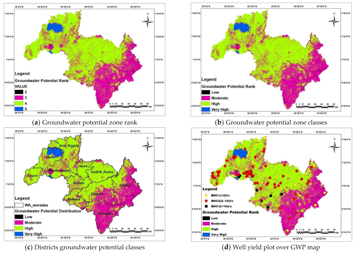
Groundwater is a crucial source of water supply due to its continuous availability, reasonable natural quality, and being easily diverted directly to the poor community more cheaply and quickly. The West Arsi Zone residents remain surface water dependent due to traditional exploration of groundwater, which is a tedious approach in terms of resources and time. This study uses remote sensing data and geographic information system techniques to evaluate the groundwater potential of the study area. This technique is a fast, accurate, and feasible technique. Groundwater potential and recharge zone influencing parameters were derived from Operational Land Imager 8, digital elevation models, soil data, lithological data, and rainfall data. Borehole data were used for results validation. With spatial analysis tools, the parameters affecting groundwater potential (LULC, soil, lithology, rainfall, drainage density, lineament density, slope, and elevation) were mapped and organized. The weight of the parameters according to percent of influence on groundwater potential and recharge was determined by Analytical Hierarchy Process according to their relative influence. For weights allocated to each parameter, the consistency ratio obtained was 0.033, which is less than 0.1, showing the weight allocated to each parameter is acceptable. In the weighted overlay analysis, from a percent influence point of view, slope, land use/cover, and lithology are equally important and account for 24% each, while the soil group has the lowest percent of influence, which accounts only 2% according to this study. The generated groundwater potential map has four ranks, 2, 3, 4, and 5, in which its classes are Low, Moderate, High, and Very High, respectively, based on its groundwater potential availability rank and class. The area coverage is 9825.84 ha (0.79%), 440,726.49 ha (35.46%), 761,438.61 ha (61.27%), and 30,748.68 ha (2.47%) of the study area, respectively. Accordingly, the western part of district is expected to have very high groundwater potential. High groundwater potential is concentrated in the central and western parts whereas moderate groundwater potential distribution is dominant in the eastern part of the area. The validation result of 87.61% confirms the very good agreement among the groundwater record data and groundwater potential classes delineated.

1. Introduction

Water is the most significant natural resource supporting human health, economic development, and ecological diversity. Groundwater is part of the water cycle, and which is stored in the saturated zones underneath the land surface and moves slowly through geologic formations called aquifers. Water could remain in an aquifer for hundreds or thousands of years. The existence and flow of groundwater is controlled by factors such as geological formations, soil type, lineament density, slope, drainage density, rainfall form, morphology, land-use/land-cover characteristics, and the interrelation between them [1,2]. Most groundwater originates from precipitation that percolate through the rock strata. Groundwater replenished, or recharged, by rain and snow melt that seep down in to the cracks and crevices beneath the land’s surface. In different areas of the world, people face solemn water scarcities because groundwater discharge for use is faster than its natural replenishment (recharge). Due to the reason that groundwater is incessantly accessed and its reasonable natural quality, it becomes a vital source of water supply, both in urban and rural areas of any country. Indeed, due to groundwater being easily diverted directly to poor communities far more cheaply and quickly than surface water, it helps in poverty mitigation and reduction.

Lately, preparing a groundwater potential district map is crucial to delineate the location of a new abstraction well to fit the increasing demand of water. Groundwater resource thematic developing helps in the optimum use and appropriate safeguarding of groundwater resources [3,4,5]. The usual method of preparing a groundwater potential thematic depends on land surveying. Currently, GIS and RS techniques made groundwater resource potential detection easier, accurate, and faster [6]. Demarking of groundwater existence locations using RS data and GIS depends on indirect investigation of the directly visible factors mentioned above. A blend of these methods had been considered to be an effective instrument in locating and mapping groundwater potential [7,8]. The Geographic Information System is a very helpful and influential instrument in demarcation of groundwater potential and scarcity zones, analyzing and quantifying multivariate features of groundwater incidence [9]. It has the power of developing information in different thematic layers and integrating them with adequate accuracy within a short period of time. Satellite imageries are progressively used in groundwater investigation due to their usefulness in categorizing various ground topographies, which may help as either direct or indirect pointers of presence of groundwater [10,11,12]. Geospatial techniques help in generating and analyzing thematic layers such as geology, topography, soil, and land use for generating groundwater potential regions map [5,13,14].

Analytic Hierarchy Process (AHP) is a concept of measurement by pairwise comparisons, which depend on judgements of professionals to originate precedence scales. The judgements are made by method of rank of absolute judgements which denotes how the elements control each other with respect to an attribute given [15]. The AHP approach is a very flexible for the reason that it produces an easy way to discover the relationship among criteria and alternatives. AHP can be made in several ways, one of which is to use proficient choice software, by which its operation and calculation stages are done automatically. In the current study, Saaty’s Analytic Hierarchy Process (AHP), which is a broadly used Multi-Criteria Decision Analysis (MCDA), was used to evaluate groundwater potential districts of regions. Decision making comprises various criteria and sub-criteria used to rank the alternatives of a decision. The criteria may be impalpable and have no measurements to help as a guide to rank the alternatives. Creating priorities for the criteria themselves in order to weigh the primacies of the options and add over all the criteria to gain the desired overall ranks of the alternatives is a thought-provoking task. In groundwater potential and recharge zone determination and groundwater potential zonation, the percent weight of factors will be calculated and determined by the AHP Excel calculator in which experts’ experiences are deemed highly important and implemented. GIS techniques were used for the weighted overlay analysis and integrated with multi-criteria analysis.

High relief and steep slopes impart higher runoff, while topographical depressions and flat areas increase infiltration. Areas with a high drainage density increase surface runoff more than areas with a low drainage density. A high lineament density produces good groundwater potential and a low lineament density produces low groundwater potential. Areas covered with forest, other vegetation, and agriculture provide cracks and loosen the soil, so infiltration will be more and runoff will be less, whereas in urban areas and bare land the rate of infiltration may decrease. Loam, silty-loam, silt, sandy-loam, sand, and loamy-sand soil textures have high permeability whereas in clay, sandy-clay, silty-clay, clay-loam, sandy-clay-loam, and silty-clay-loam the permeability is poor; in coarse granule loam the permeability is high and the flow is rapid. Areas having more rainfall have a good groundwater prospect and the areas with low rainfall have poor groundwater prospects. Geological formations that are deeply fractured, with cracks, fissures, folds, and discontinuities, are porous, which indicates high groundwater recharge prospects.

The purpose of groundwater potential modeling in this study is to identify groundwater-accessible locations throughout the study region in an easy and simple way. This will increase the accuracy and efficiency, save time, and the economy during groundwater resources management, planning, and developing by governmental and non-governmental organizations. The study was aimed to conduct (i) the demarcation of groundwater potential districts and isolation of appropriate sites for groundwater development using weighted overlay analysis techniques by means of AHP and ArcGIS; (ii) prepare thematic layers (LULC, soil, geology/lithology, rainfall, drainage density, lineament density, elevation, and slope) and reclassifying them for multicriteria overlay analysis; (iii) perform weighted overlay analysis in ArcGIS to decide on a suitable site for groundwater potential districts in the West Arsi Zone; and (iv) prepare well inventory data maps and in Excel to confirm the groundwater potential districts layers generated from the weight overlay analysis.

2. Material and Methods

2.1. Study Area Description

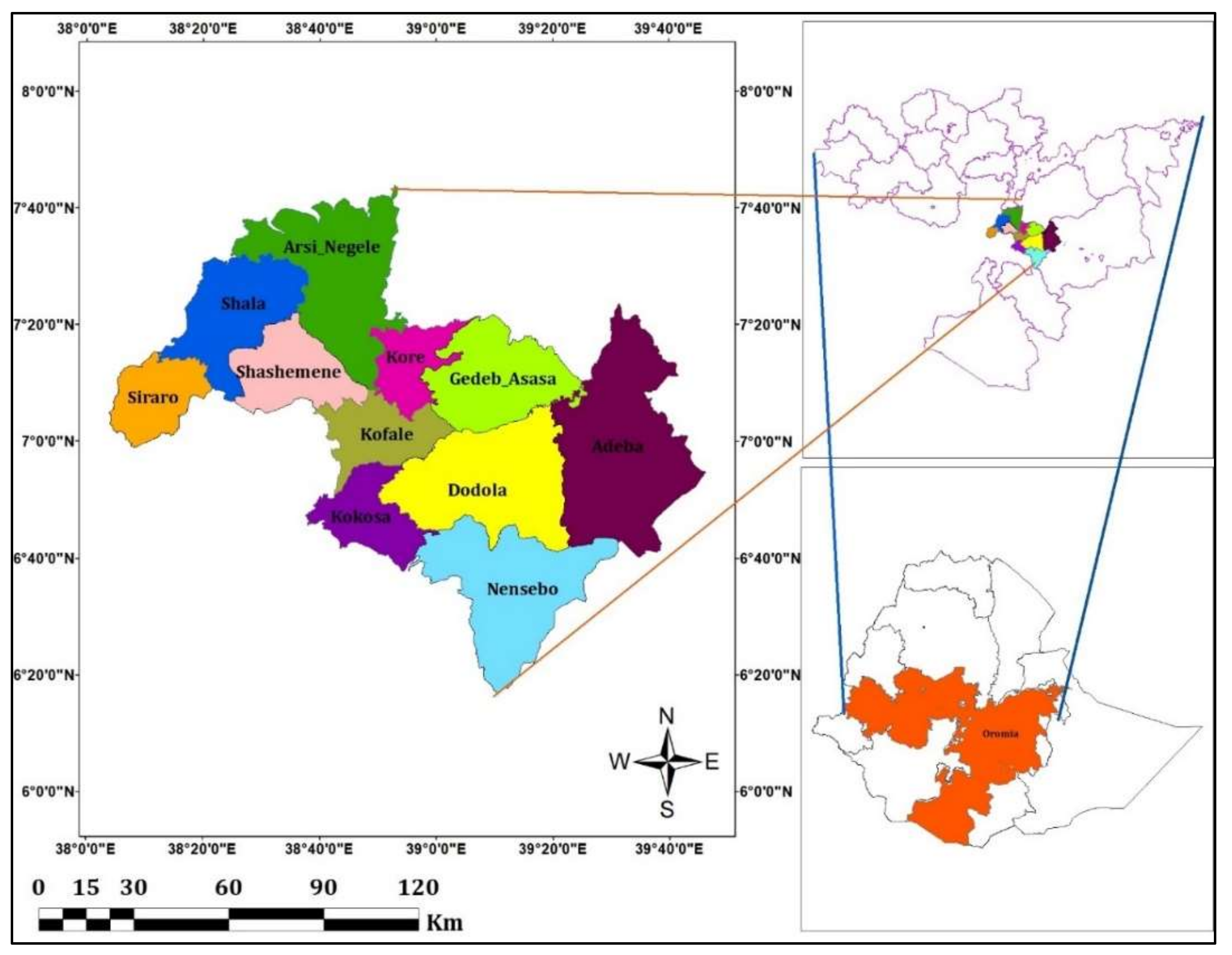
This study was conducted in West-Arsi zone; one of 20 zones of the Oromia regional government located in the central part of Ethiopia. It is situated between the 06°00′ and 08°00′ N latitudes and 38°00′ and 39°50′ E longitudes in the central part of Ethiopia (Figure 1). It covers an approximate total area of about 1,246,851.15 hectares or 12,468.51 square kilometers.

It is sub-divided into 11 districts (woredas), namely, Adaba, Arsi-Negele, Dodola, Gadab Asasa, Kokosa, Kofale, Kore, Shala, Siraro, Shashamane, and Nensebo.

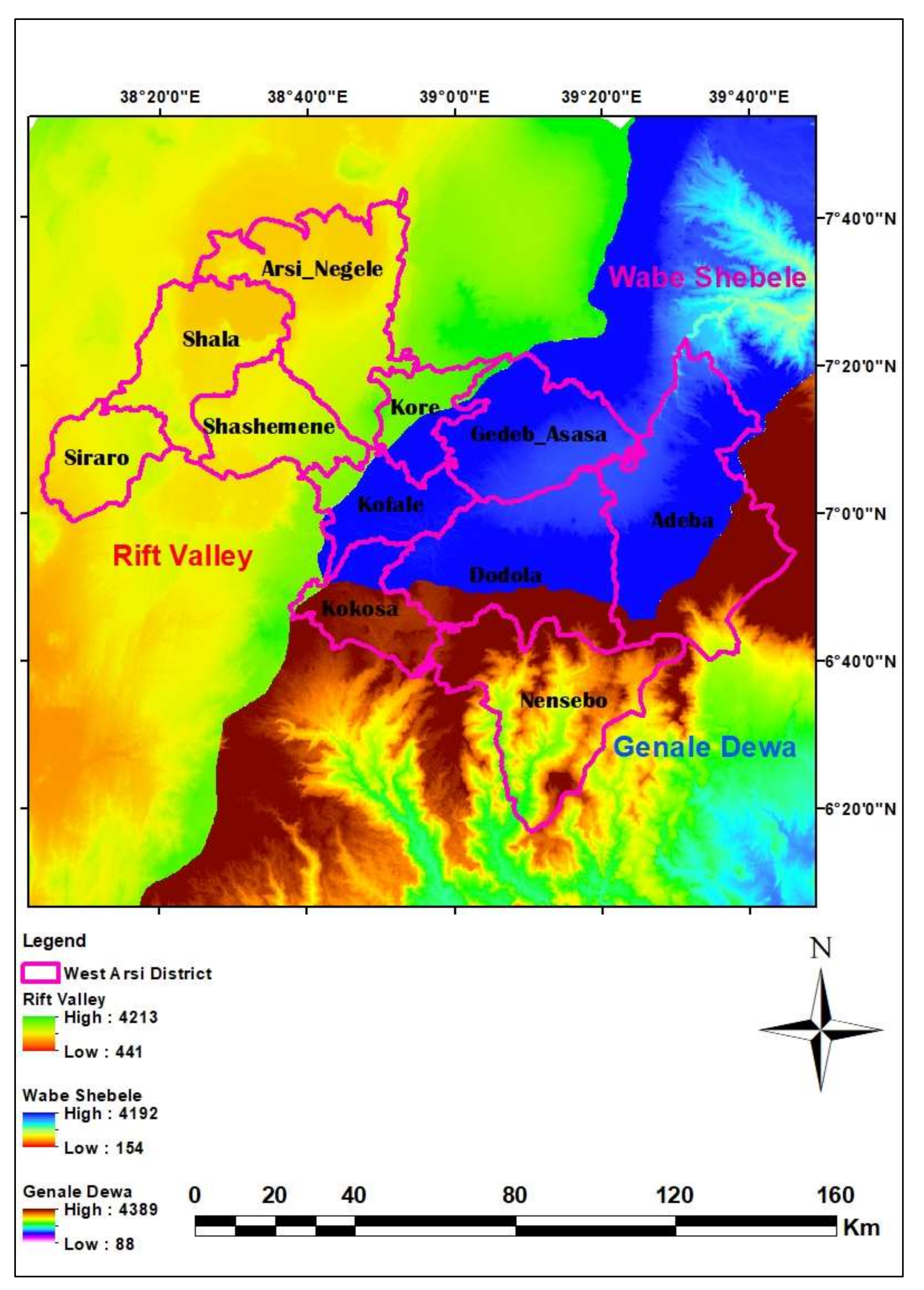
The current (2019) population of West Arsi Zone is expected to be 2,761,464, as set by the world population prospect. The area has monthly average temperatures that vary between 20 and 24 °C and annual average temperatures between 13 and 28 °C. An average altitude of an area ranges between 1464 and 4171 m. a.s.l. The yearly average annual rainfall varies between 700.5 mm and 1976.7 mm. The average sunshine hour of an area varies between 3.8 and 8.8 h/day. Annual average relative humidity and wind speed of the study area are about 71.4% and 1.4 m/s, respectively. The area is drained by three river basins; the Rift Valley Lake basin, Wabe Shebele, and Genale Dewa (Figure 2).

Hydrologically the area has a number of perennial and intermittent rivers as well as seasonal and non-seasonal springs. Lakes such as Shala, Abijata, and Langano are found in this study area. The greater part of the area is farming land with some bare land that is covered by sparsely populated natural plants (bushes; shrubs; thick, short, and long gasses; etc.) and eucalyptus plants; wheat, barley, potato, maize, teff, pea, and bean are the main product of the farming activities. The soil group of the study area is classified in to soil texture of clay, loam, sandy-loam, loamy-sand, sandy-clay, silty-clay-loam, and silt. The rock formation porosities are secondary porosities that have been developed due to weathering and tectonic fracture, which are suitable for groundwater storage and movement. The water supply source of the West Arsi Zone is rivers, springs, and hand dugs.

2.2. Methodology

2.2.1. Data Collection and Use

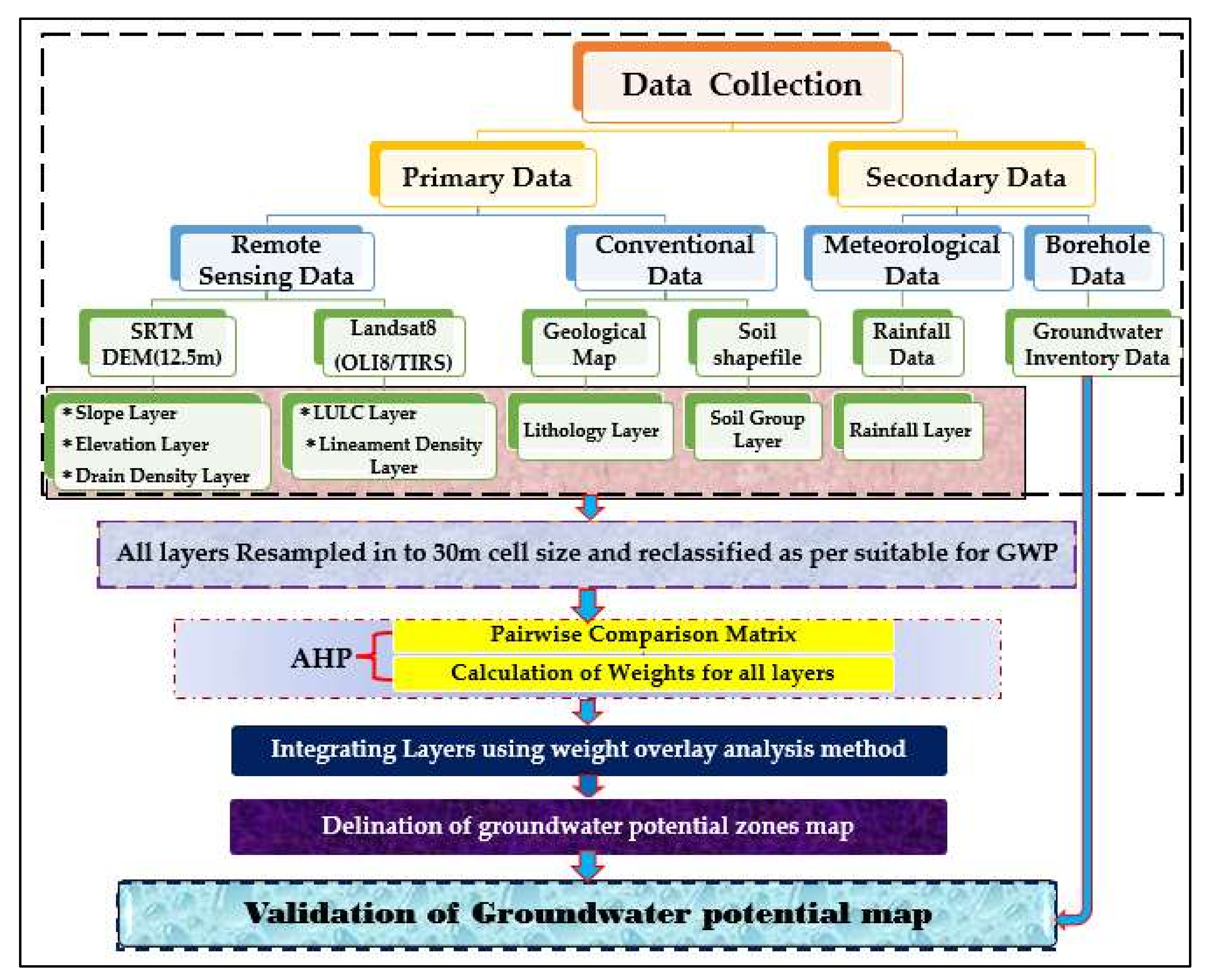
Data used for this study were collected from one-of-a-kind sectors, businesses, and extraordinary internet site sources. For this study, eight major surface and sub-surface groundwater potential-influencing criteria were separated and set for groundwater potential assessment. These criteria were selected due to being commonly used in previous literature [16,17,18,19,20,21,22,23,24] and advised by a number of experts to be used. Procedure followed to arrive at about the main objective of this study is as shown in (Figure 3).

Accordingly, based on accessible records and a literature review, eight groundwater-controlling factors were identified as proxy data, namely, slope, elevation, drainage density, lineament density, LULC, soil, rainfall, and lithology/geology. Groundwater stock records for validation purpose were additionally used. A DEM file of 30 m spatial resolution was downloaded from Image, courtesy of the USGS Earth Explorer webiste (https://earthexplorer.usgs.gov/ (accessed on 2 January 2020)) in the structure of Shuttle Radar Topographic Mission (SRTM) 1Arcsecond Global.

Operational Land Imager (OLI8)/Thermal Infrared Sensor (TIRS) with path and row of 168/055 scenes, received on 1 February 2019, and with a spatial resolution of 30 m for the seen to infrared and 15 m for the panchromatic, were downloaded from Image, courtesy of the USGS Earth Explorer (https://earthexplorer.usgs.gov/ (accessed on 22 November 2019)) website. From this source of data, slope, elevation, drain density, LULC, and lineament density layers were generated. Rainfall records were gathered from National Meteorological Agency of Ethiopia. The geology map used, at the scale of 1:1,000,000, was collected from the Geological Survey of Ethiopia and NB-37-2, 3, 6, and 7, which are the Dodola, Hosana, Asela and Dila hydrogeological maps, with notes downloaded from website https://gis.gse.gov.et/hg-maps/ (accessed on 15 April 2020). Groundwater inventory data (borehole, spring, and well data) of West Arsi Zone were from West Arsi Water, Mineral and Energy Bureau (WAWMEB). Ethiopia Soil records were gathered in the form of a shape file from the Food and Agricultural Organization [16] and Ministry of Water, Irrigation and Energy (MoWIE). The shape file to learn about the region was bought from West Arsi Zone Administrative Bureau and Oromia Administrative Bureau, used for extraction of the groundwater potential-influencing thematic layers.

2.2.2. Developing Groundwater Potential-Influencing Thematic Layers and Reclassifying

Land Use Land Cover Thematic Layer: Landsat8 OLI/TIRS has a path 168 and row 055 with cloud cover of land 0.01, Roll Angle of −0.001, Sun Azimuth of 130.39029597, Sun Elevation of 52.16321853, and spatial resolution/Cell Size of 30 m. Image composite using the process tool box from bands 1, 2, 3, 4, 5, 6, and 7 was done and the West Arsi Zone-representing image was extracted using the shapefile of study area with the help of the extraction tool of the spatial analysis tools. The LULC classification was done with help of the training sample manager tool, which was used to select the representative classes of the LULC, and the base map was used. This classification was a supervised classification because sample training was used.

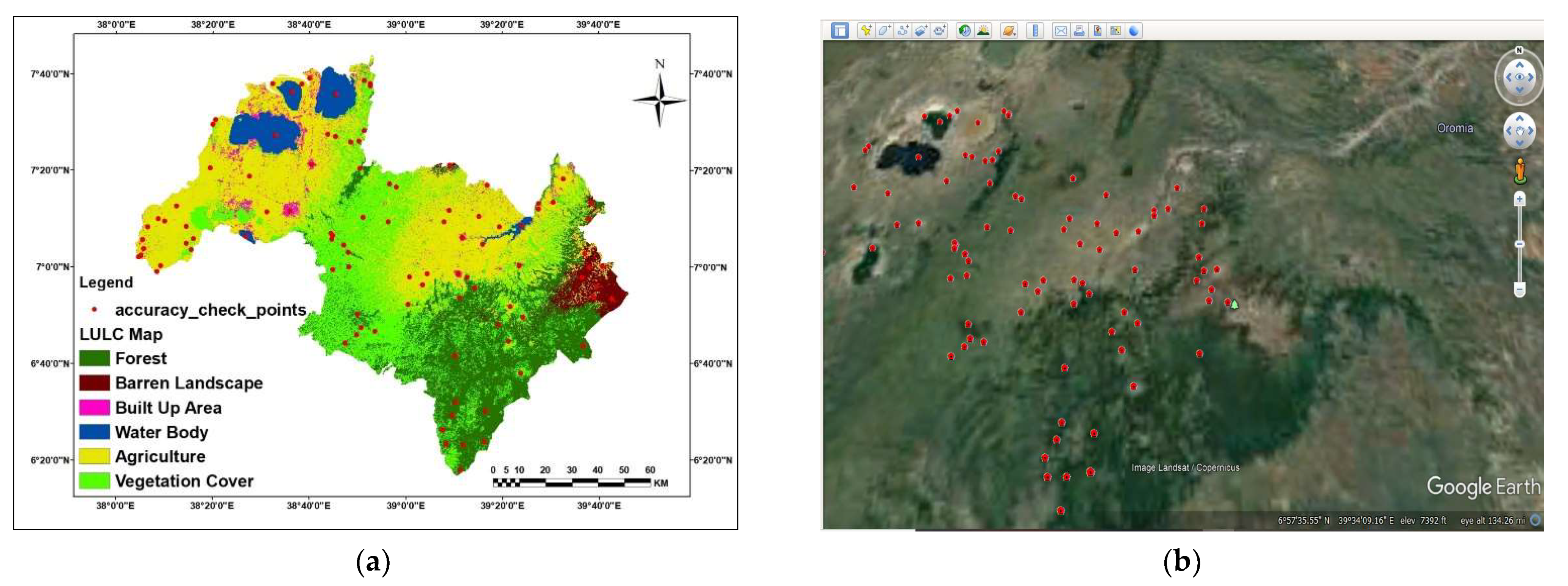
The LULC classification accuracy was checked by a hundred random points (

Table 1. Random points taken for LULC accuracy-checking purposes.

Water Body	Built-Up Area	Barren Landscape	Forest	Vegetation Cover	Agriculture
10	10	6	19	24	31

) edited on LULC-generated maps (Figure 4a) and opened on Google Earth Professional (Figure 4b). prediction accuracy, truth accuracy and overall accuracy were computed (

Table 2. LULC accuracy-checking pivot table generated in Excel.

Sum of Value	Column Labels
Row Labels	207	312	381	543	544	545	Grand Total
207	17					2	19
312	1	4				1	6
381			8		1	1	10
543				10			10
544		3			28		31
545	1				3	20	24
Grand Total	19	7	8	10	32	24	100

).

The kappa coefficient was used as a degree of agreement between the model predictions and reality [25] or to see if the values contained in a slip matrix represent a result considerably better than random [26]. The supported rating criteria for the kappa coefficient statistics, with the kappa coefficient ranging between 0.61 and 0.80 in strength agreement, are substantial, and the 0.81−1.00 strength agreement is almost perfect [27] (

Table 3. Kappa coefficient rating and strength of agreement.

Sr. No	Kappa Coefficient	Strength of Agreement
1	<0.00	Poor
2	0.00–0.20	Slight
3	0.21–0.40	Fair
4	0.41–0.60	Moderate
5	0.61–0.80	Substantial
6	0.81–1.00	Almost perfect

).

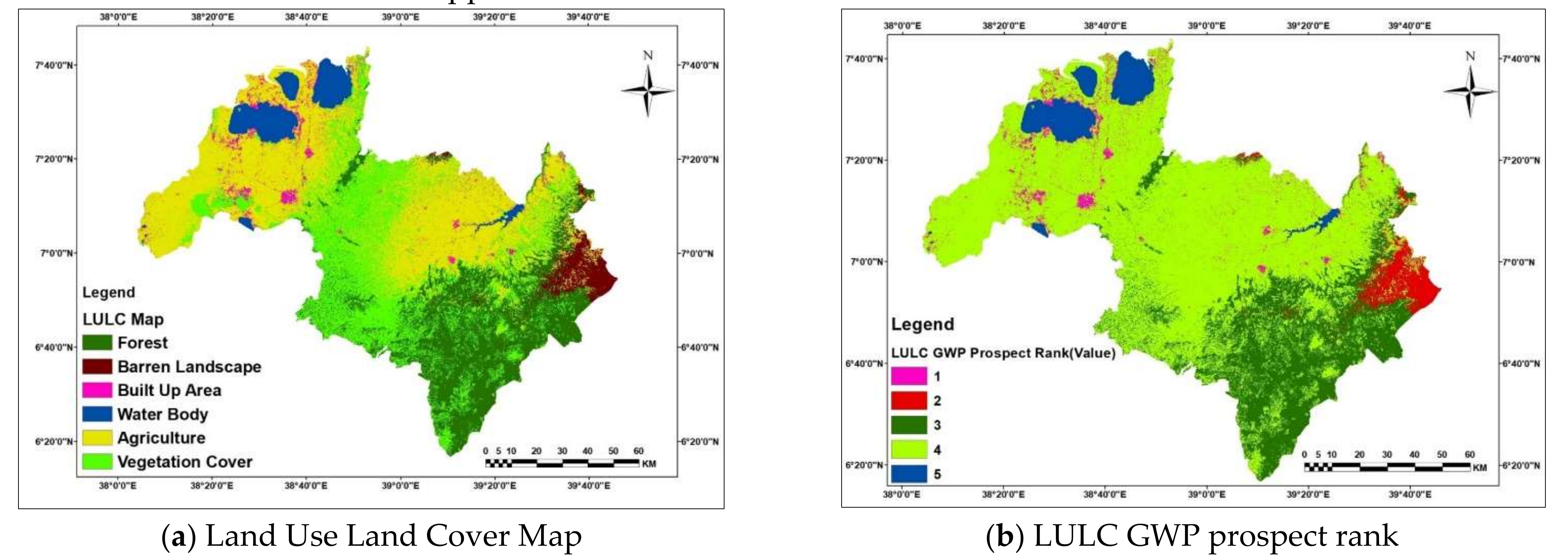
Where 207 is Forest, 312 is Barren Landscape, 381 is Built Up, 543 is Water Body, 544 is Agriculture, and 545 is Vegetation Cover. Finally, the Land-Use/Land-Cover (LULC) layer of a district was ready and reclassified in line with the suitability of the parameters for groundwater potential availability (Figure 5a,b).

$$\mathrm{OAA}=\left(\frac{\mathrm{Total} \mathrm{Properly} \mathrm{classified} \mathrm{pixels}}{\mathrm{Total} \mathrm{number} \mathrm{of} \mathrm{reference} \mathrm{pixels}}\right)100\%$$

(1)

where $\mathrm{OAA}$ is over all Accuracy

$$\mathrm{PA}=\left[\frac{\mathrm{Correctly} \mathrm{classified} \mathrm{pixels} \mathrm{in} \mathrm{each} \mathrm{category} }{\mathrm{Corresponding} \mathrm{column} \mathrm{total}}\right]100\%$$

(2)

where PA is prediction Accuracy

$$\mathrm{TA}=\left[\frac{\mathrm{correctly} \mathrm{classified} \mathrm{pixels} \mathrm{in} \mathrm{every} \mathrm{class} }{\mathrm{Corresponding} \mathrm{row} \mathrm{total}}\right]100\%$$

(3)

where TA is Truth Accuracy

$$\mathrm{Kappa} \mathrm{coefficient}\left(\mathrm{K}\right)=\left[\frac{\left(\mathrm{TCS}\ast \mathrm{TS}\right)-\sum \left(\mathrm{Ct}\ast \mathrm{Rt}\right)}{{\mathrm{TS}}^2-\sum \left(\mathrm{Ct}\ast \mathrm{Rt}\right)}\right]100\%$$

(4)

where Ct is column total, Rt is row total, TCS is total correct sample (87), and TS is total sample (100).

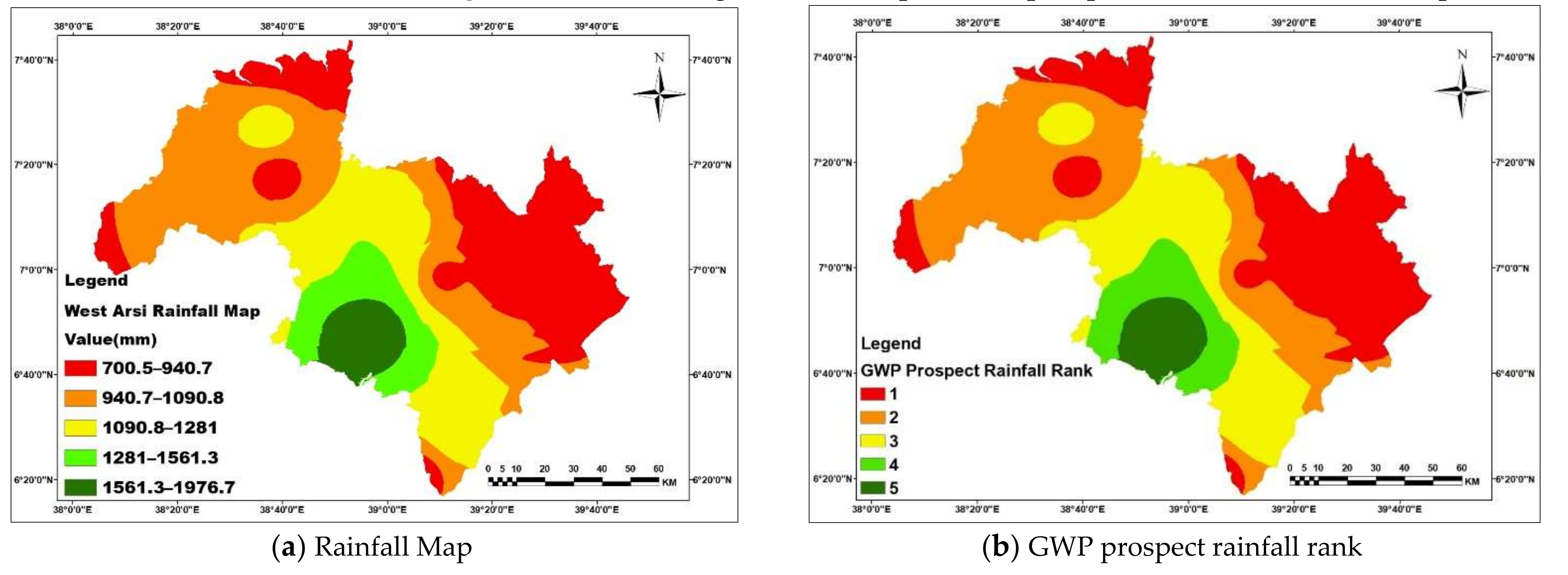
Rainfall Thematic Layer: Annual rain information of twenty-six years (1993−2019) from thirty-four stations in and from neighbors of the study space were obtained from National Earth Science Agency of the Federal Democratic Republic of Ethiopia. Annual point rain measures were regenerated to surface rain information employing a geo process tool of ArcGIS that interpolates a surface from points and rain map generated (Figure 6a). This rain map categories were reclassified into 5 category values in line with its rank as per the quality of the groundwater potential and the recharge victimization sort tool in the spatial analyst tools (Figure 6b).

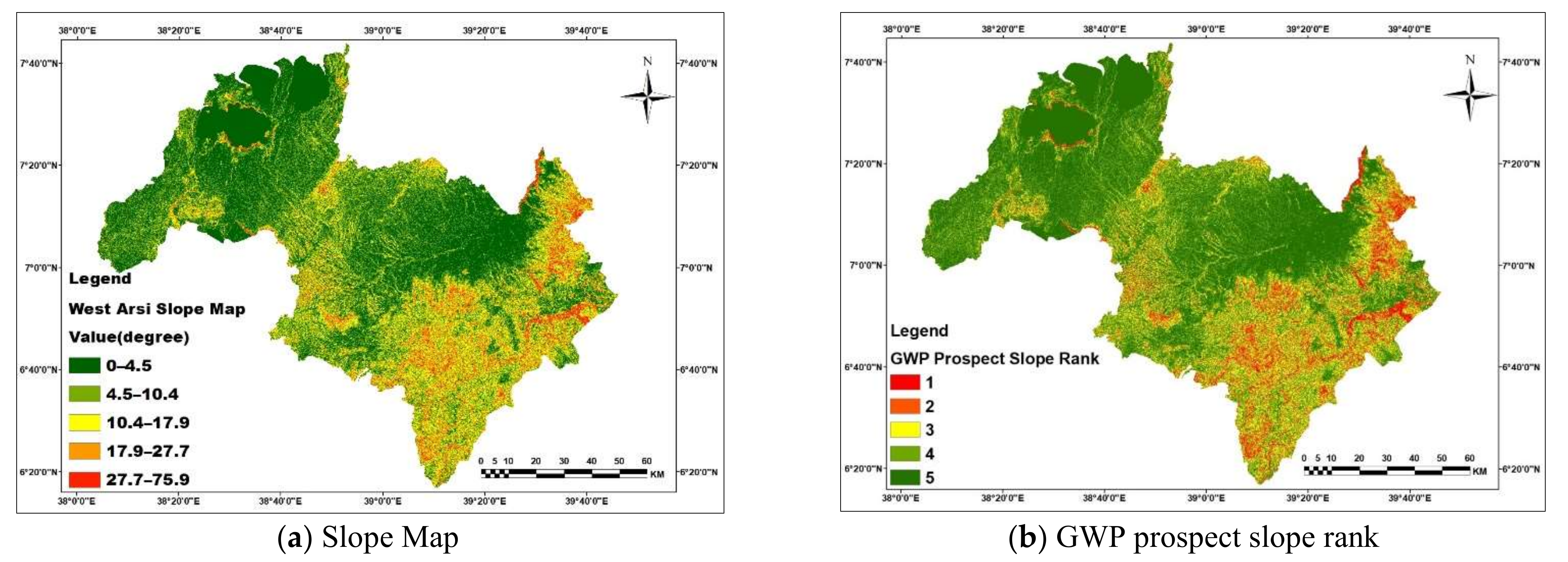
Slope Thematic Layer: Closely spaced contours represent vessel slopes and distributed contours exhibit a light slope. The slope values area unit was calculated either in percentage or degrees in each vector and formation forms. The study space DEM was extracted applying the extraction tool of the spatial analyst tools from DEM file downloaded and mosaicked to a single DEM. The slope layer of the study space was generated applying 3D analyst tools of ArcGIS from the DEM (Figure 7a). The slope tool calculates elevation change at a degree applying elevations of the encircling [28]. The slope map classification was created applying natural breaks and therefore the slope degree of the West Arsi Zone ranges from 0° to 75.9°. These slope map categories were reclassified into 5 category values, in keeping with its rank as per the suitability for groundwater potential creation by means of the class tool in the spatial analyst tools (Figure 7b).

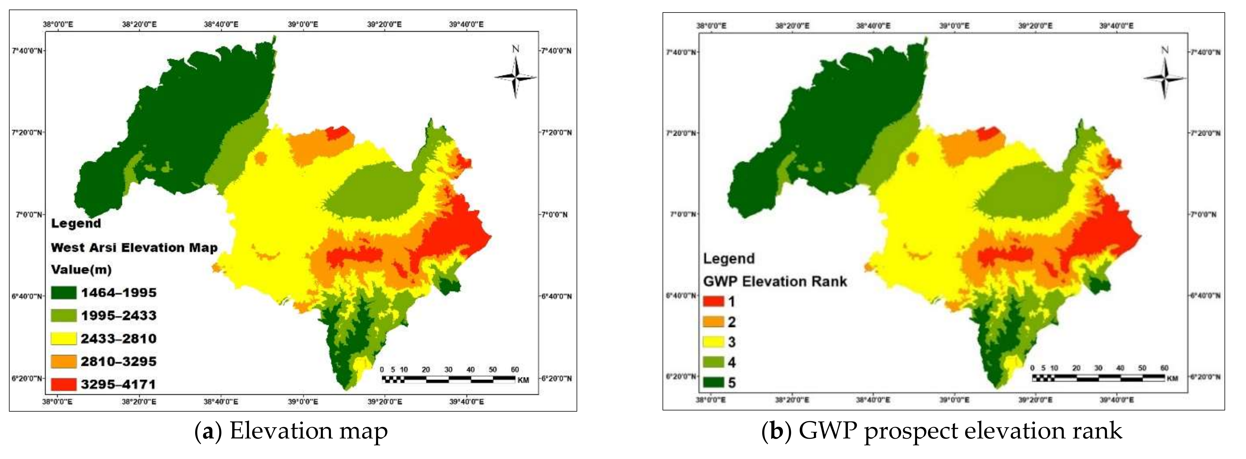
Elevation Thematic Layer: The elevation layer of the study space was generated from a DEM. Thus, the elevation information is required to be included in groundwater potential studies. The elevation layer of the West Arsi district was assessed given the 5 categories per its contribution to groundwater potential and recharge of the study space (Figure 8a). These elevation layer categories were reclassified into 5 category values per its rank as per the appropriateness for groundwater potential and recharge, applying the classify tool of the spatial analysis tools (Figure 8b).

Drainage Density Thematic Layer: The drain density (km/km²) expresses the nearness of space of waterway conduits, so providing a quantitative measuring of the typical span of waterway conduits of the entire basin [29]. To come up with a drain density map of a region, a filling sink was performed initially to get rid of the highest elevation and lowest elevation that lure the water applying the DEM manipulation tool of the terrain-preprocessing tool. A flow direction map was generated from the fill sink applying the flow direction tool of the land preprocessing tools. A flow accumulation map was generated from the flow direction applying the flow accumulation tools of the land preprocessing in Arc Hydro tools. The stream definition map was made from the flow accumulation data applying the raster calculator tool of the map algebra tool in the spatial analysis tools. A sink may be a cluster of 1 or a lot of cells that have lower elevations than all the encompassing cells whereas a peak may be a cluster of 1 or a lot of cells that have higher elevations than all the encompassing cells [30]. The drain density layer of the region has been created from a dissolved stream network applying density tool in ArcGIS spatial analyst tools (Figure 9a). The drain density layer of the study space was made applying the line density tool of the spatial analysis tools in ArcGIS software. The line density tool calculates drain density by dividing the span of the drain line by the encompassing watershed space, cells upstream of the cell, for every cell within the input flow direction grid. These drain density map categories were reclassified into 5 category values per its rank as per the suitability for groundwater potential and recharge, applying the separate tool of the spatial analysis tools (Figure 9b). Slope, elevation, and drain density maps of the space were extracted, processed, and generated from a Shuttle Radar Topographic Mission DEM of 12.5 m by 12.5 m spatial resolution, downloaded from USGS Earth explorer.

Lineament Density Thematic Layer: Lineaments are unit straight linear parts visible at the surface as a major “line of landscape” [31]. These are units primarily being a mirrored image of the discontinuities on the Earth’s surface caused by geologic or geomorphic processes [32]. Band 8 (0.50–0.68 μm), which is a panchromatic of the OLI8/TIRS image, was downloaded from USGS Earth explorer (https://earthexplorer.usgs.gov/ (accessed on 22 November 2019)) website and had a spatial resolution of 15 m extracted applying the West Arsi Zone shape file and exported in word format of the stretched sort. Lineament of a picture was extracted mechanically from images exported in .tiff format applying PCI Geomatica Banff applying the line tool in the algorithmic librarian tool saved as file sort Arc read. Line split, line split at vertices, and lineament density maps were generated applying the editor tool, feature tool of data management tool, and density tool of the spatial analysis tool operation. Principal Component Image (PCI) carry most data and is appropriate for lineament extraction functions. Band 8 of Landsat 8 was chosen and used because of its ability to identify linear and curvilineal features and having higher spatial resolution of 15 m and it is panchromatic mirrored band. Finally, the lineament and reclassified lineament density layer was produced from the band 8 OLI8/TIRS image (Figure 10a). These lineament density map categories were reclassified in to 5 category values in line with its rank as per suitable for groundwater potential and recharge zone delineation, applying the reclassify tool of the spatial analysis tools (Figure 10b).

Soil Group Thematic Layer: Soil group map (Figure 11a) of West Arsi Zone was generated from the dissolved shapefile of the study area clipped from the Ethiopia soil group shapefile using the clip tool of the analysis tools and converted into a raster using the polygon-to-raster tool of the conversion tools. This soil group map was regrouped into different six soil group texture and permeability. These soil map classes were reclassified in to five class values according to its rank as per the suitability for groundwater potential formation using the reclassify tool of the spatial analyst tools and a new soil group map was generated (Figure 11b).

Lithological Map Preparation: The lithology layer of the region was generated by geo-referencing, digitizing, extracting of a region formation from the geological layer of the Oromia 1:1,000,000 scale [33] obtained from the Geological Survey of Ethiopian (GSE). The geology layer of Oromia was georeferenced applying geo-referencing tool of ArcGIS and corrected, and projected to the WGS1984 UTM Zone 37, applying projection and transformation tools of the data management tools. The West Arsi Zone geological formation image was clipped applying the study space shapefile with the assistance of clip tool of the analysis tools of ArcGIS. Study space lithology layer was generated from dissolved geology shape file reborn to raster applying conversion using the polygon-to-raster tool of the conversion tools (Figure 12a). The lithology layer categories were reclassified into 5 category values per its rank as per the suitableness for groundwater potential formation applying the reclassify tool of the spatial analysis tools, and a new lithology layer (Figure 12b) was generated.

Each influence layer was ready and reclassified in to 5 categories in an exceeding manner, which will support the general goal of groundwater potential and recharge zone mapping. These maps layers were projected onto an equivalent reference system, resampled into an equivalent formation layer of 30 m cell size, and reclassifying all the thematic layers’ individual parameters as appropriate for groundwater potential zonation so as to be acceptable for the weight overlay analysis. All the desired thematic maps were developed from the collected datasets applying MS-Excel, ArcGIS 10.3.1 version, PCI geomatica Banff, and the ERDAS IMAGINE 2015 package. The spatial resolution of reclassified precipitation, slope, elevation, drain density, lineament density, LULCr, soil, and lithology map was 30 m × 30 m and with a 10,000 m² to hectare conversion factor. Accordingly, the area coverage of these categories will be calculated using the formula

$$\mathrm{Area}\left(\mathrm{ha}\right)=\frac{\mathrm{Pixel} \mathrm{Count}\times 30 \mathrm{m}\times 30 \mathrm{m}}{10,000 {\mathrm{m}}^2}$$

(5)

Area in percent will be calculated using the formula

$$\mathrm{Area}\left(\%\right)=\frac{\mathrm{Row} \mathrm{Area} }{\mathrm{Total} \mathrm{Area} }\times 100$$

(6)

In groundwater potential influencing parameters (rainfall, slope, elevation/altitude, drain density, and lineament density layers classification), there is no onerous and quick rule for groundwater potential and recharge or runoff generation. Hence, merely the natural break on the ArcGIS ArcMap classified, which show the kind that existed by default, was applied.

2.2.3. Analytical Hierarchy Process to Assign Weight

Among the numerous techniques, the Analytical Hierarchy Process (AHP) enables plenty to systematically discover the maximum influencing parameters [12,22,34,35,36]. The Analytical Hierarchy Process (AHP), proposed by [37], is the regularly used approach for groundwater potential mapping. The eight criteria/elements (rainfall, lithology, lineament density, land use/land cover, soil group, slope, elevation, and drain density) predicted to affect groundwater distribution of the West Arsi sector were separated and set for weight overlay. A pairwise comparison matrix, P(m × m), of which m is the number of parameters to be in comparison, was changed to being built primarily based totally on the quantity of the entered elements for delineation of the groundwater potential and recharge zones [38]. Ordering and assigning a scale for parameters (elements) affecting the groundwater potential calls for a review of the variety of literature, personal judgments, and professional opinion.

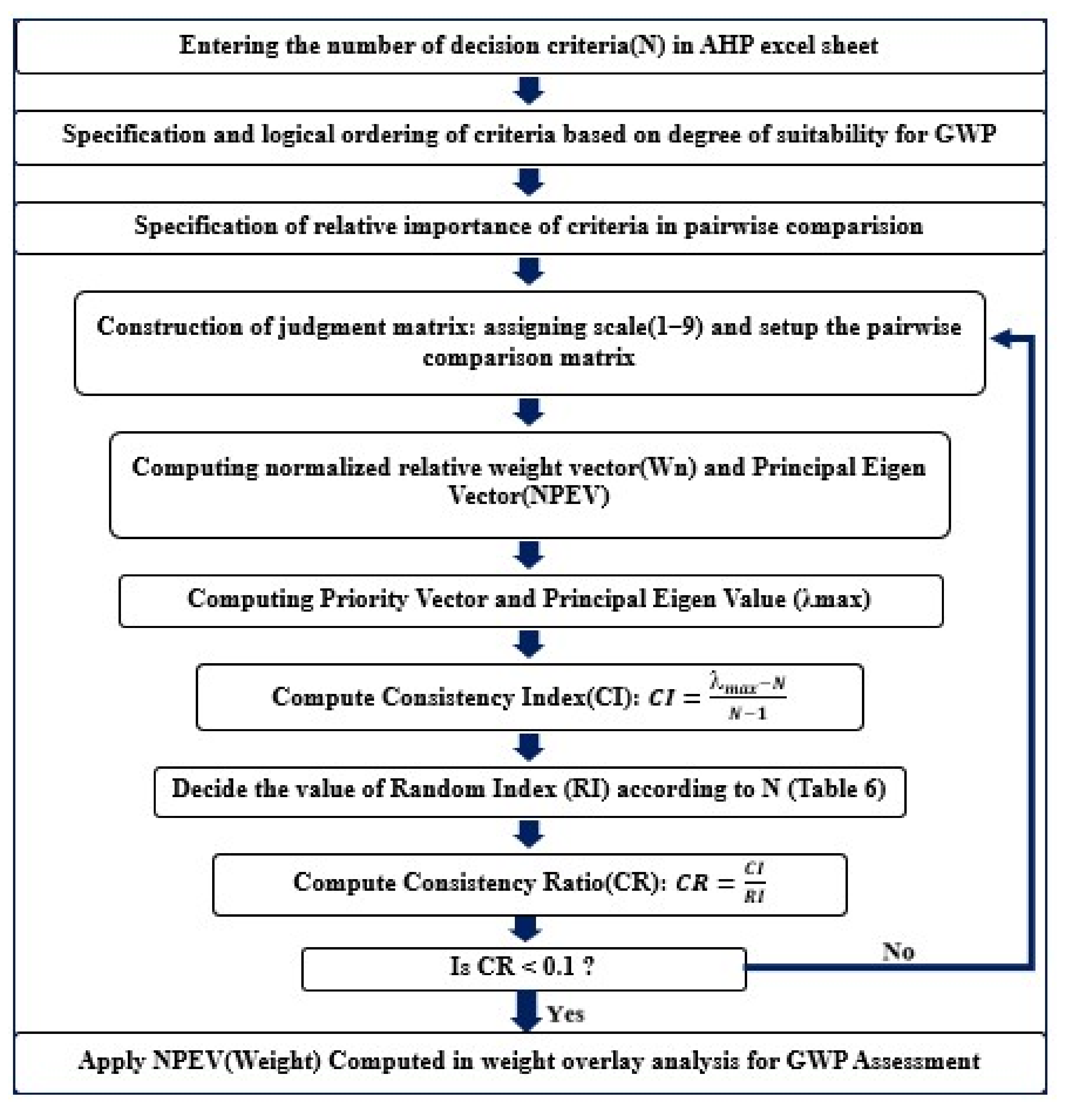
The main purpose of AHP in this study was to determine the appropriate Normalized Principal Eigen Vector (NPEV) or Percent Weight in ArcGIS environment in the weight overlay analysis. Generally, the procedure followed to determine and validate the normalized principal eigenvector is shown in (Figure 13).

Before placing the criterion into pairwise comparison and assigning the scale for groundwater potential assessment, first all of the elements need to be in a logical order in the AHP Excel sheet, primarily based on the degree of suitability for groundwater potential and recharge zone contribution (

Table 4. Analytical Hierarchy Process pairwise comparison matrix of the thematic layers and scale assigned.

		Criteria			More Important?	Scale
i	j	A		B	A or B	(1–9)
1	2	Slope		LULC	A	1
1	3			Lithology	A	1
1	4			Elevation	A	3
1	5			Drainage Density	A	3
1	6			Lineament Density	A	5
1	7			Rainfall	A	7
1	8			Soil	A	9
2	3	LULC		Lithology	A	1
2	4			Elevation	A	3
2	5			Drainage Density	A	3
2	6			Lineament Density	A	5
2	7			Rainfall	A	7
2	8			Soil	A	9
3	4	Lithology		Elevation	A	3
3	5			Drainage Density	A	3
3	6			Lineament Density	A	5
3	7			Rainfall	A	7
3	8			Soil	A	9
4	5	Elevation		Drainage Density	A	1
4	6			Lineament Density	A	3
4	7			Rainfall	A	3
4	8			Soil	A	5
5	6	Drainage Density		Lineament Density	A	1
5	7			Rainfall	A	3
5	8			Soil	A	5
6	7	Lineament Density		Rainfall	A	1
6	8			Soil	A	3
7	8	Rainfall		Soil	A	1

). In this study, primarily based on the features of the area under study and suitability of the criteria elements for groundwater potential and recharge zone contribution, all of the parameters are ordered. Slope and elevation decide the destiny of the water that reaches the floor of the earth. From slope conduct of the west Arsi Zone, about 72.41% of the vicinity is appropriate for groundwater potential and recharge of surface water whilst in comparison to the rest of the criteria under consideration. This suggests that about 72.41% of a place is almost flat to mildly sloped, which permits extra rainfall or surface water to percolate and infiltrate.

Therefore, consistent with this study, slope is located at the start order. Area protected through water body, vegetation, and agricultural location are maximally appropriate for surface water percolation. Especially agricultural and vegetation protected areas trap the water, reduces runoff, and will increase infiltration. The overall sum of area protected through a water body, agriculture, and vegetation makes a contribution to about 71.67% of a place and puts LULC at the second order subsequent to slope in phrases of suitability of the criteria for groundwater potential and recharge zone. Geology/lithology performs an essential function in the occurrence and distribution of groundwater in any terrain [39] due to the fact water might recharge aquifers directly. A 66.2% lithology of a place is appropriate for groundwater potential, which places it in the third order in terms of suitability of the criteria for groundwater potential. Elevation was 49.02% appropriate for groundwater potential and thus placed in the fourth order accompanied by drainage density, which contributes 46.32% to high and very high groundwater potential. In phrases of lineament density, only 27.94% of a place is appropriate for surface water percolation, recharge, and groundwater potential formation. Therefore, groundwater potential is low regarding lineament density areas and consequently lineament density is located in the 6th order.

Rainfall performs an essential function for hydrologic cycle and controls groundwater potential [40]. Rainfall performs an important function in the occurrence of groundwater. It is clear that greater rainfall might also additionally reason greater recharge ability, even though that ability is challenged through different constraining elements, including slope, geology, land use/cover, drainage density, lineament density, and others. Therefore, excessive recharge vicinity does now no longer always mean excessive groundwater potential areas [41]. Knowing the nature and characteristics of rainfall might also additionally allow one to conceptualize and predict its outcomes on runoff, infiltration, and groundwater potential and recharge [42]. The opportunity of groundwater recharge might be excessive on the location in which the rainfall is excessive and is low in which rainfall is low [41,43,44,45]. Regions that obtain greater rainfall have greater possibility of infiltration than districts with low precipitation [40]. From a rainfall factor view, only 13.85% of a place gets high and very high rainfall; consequently, in terms of rainfall, only 13.85% of a place will have high and very high groundwater potential. This displays that rainfall contribution for groundwater potential formation and recharge sector could be very low and positioned in the 7th place, as compared to slope, LULC, lithology, elevation, drainage density, and lineament density.

Soil kind and texture additionally determine the infiltration ability and permeability. In phrases of the soil group, only 7.3% is anticipated to have high and very high groundwater potential and recharge, and is thus positioned in the last place in this study. This displays that about 92.7% of the soil group of a place is impermeable and will increase surface runoff and reduce infiltration. Factor effects on every different one, based on Saaty’s one to nine factor scale, were used, where 1 represents both parameters being similarly essential and nine suggests one parameter is extraordinarily essential over the alternative in phrases of goal influence [40]. The summary of this hierarchy and pairwise comparison and the assigned scale using the AHP Excel sheet is given in

Table 5. Analytic hierarchy process pairwise comparison matrix and the assigned scale.

Matrix	SL	LULC	Lith	El	DD	LD	RF	SG
SL	1	1	1	3	3	5	7	9
LULC	1	1	1	3	3	5	7	9
Lith	1	1	1	3	3	5	7	9
El	1/3	1/3	1/3	1	1	3	3	5
DD	1/3	1/3	1/3	1	1	1	3	5
LD	1/5	1/5	1/5	1/3	1	1	1	3
RF	1/7	1/7	1/7	1/3	1/3	1	1	1
SG	1/9	1/9	1/9	1/5	1/5	1/3	1	1
Column Total of PCM	4.120635	4.120635	4.120635	11.86667	12.53333	21.33333	30	42

, generated from the AHP Excel sheet and pairwise comparison matrix.

Where RF represents rainfall, SG represents soil group, LD represents lineament density, Lith represents lithology, LULC represents land use/land cover, Sl represents slope, El represents elevation, and DD represents drainage density.

Normalized Relative Weight (Wn), Eigenvector, and Normalized Principal Eigenvector (NPEV) are determined as step below.

AHP employs experts’ opinion; the role of Eigenvectors and Eigenvalues is to lessen noise withinside the records and additionally assist in decreasing over-fitting [46]. The Eigenvector is the ordering of parameter impact on groundwater potential and recharge with the aid of using assigning the weights [47]. The Eigenvector was computed to display the comparative weights of every parameter in the direction of groundwater potential and recharge [48] (

Table 6. Normalized relative weight and Normalized Principal Eigen Vector (NPEV).

Matrix	Normalized Relative Weight Vector (Wn)								Eigenvector	NPEV (%)
	SL	LULC	Lith	El	DD	LD	RF	SG
SL	0.242681	0.242681	0.242681	0.252809	0.239362	0.214286	0.233333	0.214286	0.24	24
LULC	0.242681	0.242681	0.242681	0.252809	0.239362	0.214286	0.233333	0.214286	0.24	24
Lith	0.242681	0.242681	0.242681	0.252809	0.239362	0.214286	0.233333	0.214286	0.24	24
El	0.080894	0.080894	0.080894	0.08427	0.079787	0.128571	0.1	0.119048	0.09	9
DD	0.080894	0.080894	0.080894	0.08427	0.079787	0.128571	0.1	0.119048	0.09	9
LD	0.048536	0.048536	0.048536	0.02809	0.079787	0.042857	0.033333	0.071429	0.05	5
RF	0.034669	0.034669	0.034669	0.02809	0.026596	0.042857	0.033333	0.02381	0.03	3
SG	0.026965	0.026965	0.026965	0.016854	0.015957	0.014286	0.033333	0.02381	0.02	2
Total	1	1	1	1	1	1	1	1	1	100

).

Steps followed to calculate Wn, Eigenvector, and NPEV:

• Row 1–9 of Table 5 was generated from the AHP Excel sheet.
• Scale values (Column 2–9 of Table 5) of the pairwise comparison matrix was summarized (Row 10 of Table 5).
• Normalized Relative Weight Vector (Wn) of Table 6 from Row 3–10 of Column 2–9 was computed from division of each column criterion value of Table 5 (Column 2–9 of Row 2–9) by column total (Row 10) of Table 5.
• Each Eigenvector value (Column 10 of Row 2–9) of Table 6 is the average of each row.
• Normalized Principal Eigen Vector (NPEV) of Table 6 from Row 3–10 of Column 11 is a multiply of the Eigenvector values by 100%.
• The column sum of the normalized relative weight vector (Wn) and Eigenvector is equal to 1 and Normalized Principal Eigen Vector (NPEV) is equal to 100% (Row 11 of Table 6).

The consistency ratio (CR) is used for assessment of matrix consistency. AHP includes a powerful approach used for checkup the consistency of the evaluations made through the decision maker whilst constructing every of the pairwise comparison matrix concerned within the process. Inconsistencies in pairwise comparisons grow with the growing number of comparisons [49]. For the estimation of the consistency ratio (CR), the following stages is involved:

• Priority vector (column 4 of

  Table 7. Principal Eigenvalue (λ_max) and priority vector.

  Thematic Criterion	Column Total of PCM	Eigenvector	Priority Vector
  SL	4.120635	0.24	0.969440451
  LULC	4.120635	0.24	0.969440451
  Lith	4.120635	0.24	0.969440451
  El	11.86667	0.09	1.118962872
  DD	12.53333	0.09	1.181825955
  LD	23.33333	0.05	1.169888994
  RF	30.00000	0.03	0.970094234
  SG	42.00000	0.02	0.971951575
  Principal Eigenvalue (λmax)			8.321044984

  ) for criterion is calculated by multiplying the column total of pairwise comparison matrix by Eigenvector.
• Principal Eigenvalue (λ_max) is summation of priority vector (Row 10 of Table 7).
• Consistency Index (CI) is the ratio of the distinction among the Principal Eigenvalue (λ_max) and the number of criteria (m) to number of criteria under investigation (m) less one.
• Random index (RI) was determined from

  Table 8. Random Index (RI) belongs to the number of assessment criteria (m).

  m	1	2	3	4	5	6	7	8	9	10
  RI	0	0	0.58	0.9	1.12	1.24	1.32	1.41	1.45	1.49

  of Satty (1990), which depends on number of criteria (m) considered.
• Consistency ratio (CR) is the ratio of the consistency index (CI) to the random index (RI).

The sum of the priority vector, known as the Principal Eigenvalue (λ_max), is a degree of matrix deviation from consistency [48].

According to [49], a pairwise contrast matrix exists only if the Principal Eigenvalue (λ_max) is extra than or equal to the number of the parameters investigated/criteria (m). In any other case a brand-new matrix is required. If there may be any inconsistency within the experts’ opinions, a difference among m and λ_max is indicated. Therefore, λ_max—n may be classed as a measure of inconsistency. A perfectly regular decision maker has to continually obtain CI = 0; however, small values of inconsistency can be tolerated if the consistency ratio (CR) < 0.1 [37]. The consistency index (CI) for groundwater potential and recharge zone parameters investigated in this study was calculated by the equation below.

$$\mathrm{CI}=\frac{{\mathsf{\lambda }}_{\max }-\mathrm{m}}{\mathrm{m}-1 }$$

(7)

where m is the number of assessment criteria (thematic layers in the case of this study) and λ is the Principal Eigenvalue of judgment matrix as set through Satty (1995). RI relies on the range of the criteria being compared, as shown in Table 8 [49].

From this table for m = 8, RI = 1.41. Analytical Hierarchy Process takes the consistency ratio (CR) figure among zero and 0.1 or 10%; a value greater than 10% invites for modification of comparisons.

$$\mathrm{CR}=\frac{\mathrm{CI}}{\mathrm{RI}}$$

(8)

Consistency Ratio (CR) calculation is to confirm the consistency of the judgements. Saaty (1995) advised a different consistency ratio value for different consistent pairwise evaluation matrix sizes. The recommended consistency ratio value for a three × three matrix is much less than 0.05, a four × four matrix is 0.09, and for large matrices it is recommended 0.1 [38].

2.2.4. Weighted Overlay Analysis

During the weighted overlay analysis, the ranks were given for all parameters of all thematic layers set for the study and the weight is assigned in line with their relative effect of the different parameters on groundwater potential applying the Analytic Hierarchical Process (AHP) technique [48]. After assigning weights to all thematic layers, ranks/scale values from 1 to 5 were given for the sub-variable of every thematic layer, in line with their significance for groundwater potential occurrence. According to this study, 1 represents less vital and 5 represents more vital for groundwater potential and recharge. The most worth is given to the feature expected with maximum groundwater potentiality and the minimal given to the lowest groundwater potentiality feature (

Table 9. Groundwater potential prospect rainfall map classes.

Rainfall Classes (mm)	Value (Rank)	GWP Prospect Rank	Count	Area (ha)	Percent Area
700.5–940.7	1	Very low	4,092,491	368,324.2	29.54
940.7–1090.8	2	Low	4,551,345	409,621.1	32.85
1090.8–1281	3	Moderate	3,241,868	291,768.1	23.4
1281–1561.3	4	High	1,220,442	109,839.8	8.81
1561.3–1976.7	5	Very High	747,753	67,297.77	5.4

,

Table 10. Groundwater potential prospect reclassified slope map information.

Slope Classes (Degree)	GWP Prospect Rank	Value (Rank)	Count	Area (ha)	Area (%)
27.7–75.9	Very Low	1	40,4616	36,415.44	2.93
17.9–27.7	Low	2	1,166,148	104,953.32	8.43
10.4–17.9	Moderate	3	2,243,511	201,915.99	16.23
4.5–10.4	High	4	4,274,118	384,670.62	30.91
0–4.5	Very High	5	5,737,163	516,344.67	41.50

,

Table 11. Groundwater potential prospect reclassified elevation map information.

Elevation Classes (m)	GWP Prospect Rank	Value (Rank)	Count	Area (ha)	Area (%)
3295–4171	Very Low	1	928587	83,572.83	6.70
2810–3295	Low	2	1681472	151,332.48	12.14
2433–2810	Moderate	3	4452576	400,731.84	32.14
1995–2433	High	4	2589305	233,037.45	18.69
1464–1995	Very High	5	4202042	378,183.78	30.33

,

Table 12. Groundwater potential prospect reclassified drainage density map information.

DD Class (km/km2)	GWP Prospect Rank	Value (Rank)	Count	Area (ha)	Area (%)
1.3–1.8	Very Low	1	1,286,764	115,808.76	9.29
1.0–1.3	Low	2	2,926,141	263,352.69	21.12
0.7–1	Moderate	3	3,223,861	290,147.49	23.27
0.4–0.7	High	4	3,645,417	328,087.53	26.31
0–0.4	Very High	5	2,771,782	249,460.38	20.01

,

Table 13. Groundwater potential prospect reclassified lineament density map information.

L.d Classes (km/km2)	GWR Prospect Rank	Value (Rank)	Count	Area (ha)	Area (%)
0–0.4	Very Low	1	3663565	329,720.85	26.45
0.4–0.8	Low	2	3706704	333,603.36	26.76
0.8–1.2	Moderate	3	2611845	235,066.05	18.85
1.2–1.6	High	4	2617700	235,593	18.89
1.6–2.7	Very High	5	1254151	112,873.59	9.05

,

Table 14. Groundwater potential prospect reclassified LULC map information.

Class Name	GWP Prospect Rank	Value (Rank)	Count	Area (ha)	Area (%)
Built Up Area	Very Low	1	403,696	36,332.64	2.92
Barren Landscape	Low	2	456,928	41,123.52	3.30
Forest	Moderate	3	3,062,368	275,613.12	22.11
Agriculture & Vegetation	High	4	9,206,823	828,614.07	66.48
Water Body	Very High	5	718,378	64,654.02	5.19

,

Table 15. Groundwater potential prospect reclassified soil group map information.

Soil Group	GWR Prospect Rank	Value	Count	Area (ha)	Area (%)
Eutric Cambisols/Pellic Vertisols/Orthic Solonchaks/Chromic Vertisols/Chromic Cambisols/Mollic Gleysols	Very Low	1	5,905,315	531,478.4	42.63
Dystric Histosols	Low	2	16,214	1459.26	0.12
Vitric Andosols/Mollic Andosols/Chromic Luvisols/Eutric Nitisols/Eutric Regosols/Orthic Luvisols	Moderate	3	6,921,369	622,923.2	49.96
Leptosols/Calcic Xerosols	High	4	197,857	17,807.13	1.43
Calcic Fluvisols/Calcaric Fluvisols/Eutric Fluvisols	Very High	5	813,210	73,188.9	5.87

and

Table 16. Groundwater potential prospect reclassified lithology map information.

Lithology Name	GWR Rank Prospect	Value	Count	Area (ha)	Area (%)
Qwo	Very Low	1	42,032	3782.88	0.30
gt/Pra/PRr/Qwpu	Low	2	418,592	37,673.28	3.02
Pna/PRw/Qdi/Qdp/Qwa	Moderate	3	4,221,989	379,979.01	30.48
Nc/Ncb/Nn/Qb/Qwbp	High	4	7,358,588	662,272.92	53.12
QI	Very High	5	1,811,535	163,038.15	13.08

).

2.2.5. Groundwater Potential Map Development

The groundwater potential layer was developed via way of means of overlapping the determinant groundwater contributing thematic layers. A weighted overlay analysis device was used to develop the groundwater potential map and to compute the groundwater potential index values. The reclassified layers of rainfall, lithology, slope, elevation, lineament density, drain density, soil group, land use/land cover, and their corresponding percentage, have an impact on groundwater potential, and have been included to produce a map of the spatial distribution of the groundwater potential districts inside the West Arsi space with the help of the weighted overlay tool in ArcGIS software. Weighted Overlay analysis device reclassifies values within the enter raster layers right into a common assessment scale of 1, 2, 3, 4, and 5—very low, low, moderate, high, and very high, respectively—via way of means of multiplying the cell values (rank) of every factor class via way of means of the factor weight and sums the resulting cell values collectively to produce a map of groundwater potential zones, as given by the following equation (Raviraj 2017; ESRI 2015).

$$\mathrm{GWPI}=\mathrm{RFwRFr}+\mathrm{LDwLDr}+\mathrm{LULCwLULCr}+\mathrm{SwSr}+\mathrm{EwEr}+\mathrm{SGwSGr}+\mathrm{LiwLir}+\mathrm{DDwDDr}$$

(9)

where GWPI represents groundwater potential, RF represents rainfall, LD represents lineament density, LULC represents land use/land cover, S represents slope, E represents elevation, SG represents soil group, Lith represents lithology, DD represents the drain density index and the subscript w and r represent weight and rank, respectively [50]. The GWPI values were used to categorize whether or not a place may be very high, high, moderate, low, or very low with respect to groundwater potential [1,51].

2.2.6. Validation of Groundwater Potential Occurrence Zone Map

For validating the anticipated groundwater potential zone map, an attempt was made to acquire current data from different sources for validation. Overall, 113 current groundwater inventory borehole data points were accrued from West Arsi water, mineral and energy office. Additional sources from Dodola-Goba, Hosaina, Dila, and Asela hydrogeology annexes and notes were also used. For the cause of evaluation or assessment of the qualitative consequences of the groundwater potential zones, well yield was decided on as a higher candidate than different current data. Although there is no standard category scheme, well yields may be grouped into a few category schemes, considering the particular site conditions.

According to the hydrogeology notes of the above cited maps and others, the aquifer yields that exist on this hydrogeology are in a different way categorized. Some classify as zero–three L/s: low, three—6 L/s: moderate, 6–20 L/s: high and greater than 20 L/s as very high groundwater potential zones. Others classify as 0.5–1 L/s low, 1–five L/s moderate to low and five−25 L/s high groundwater potential areas. For this study with a few changes the water point inventory categorized as less than 2 L/s was classified as low (33 boreholes), 2 to 10 L/s moderate (69 boreholes), and more than 10 high yield (11 boreholes). Borehole inventory facts were mapped on groundwater potential map; percentage of agreement was calculated and validation of the groundwater thematic map with groundwater inventory facts was done (Figure 14d). Groundwater potential prediction accuracy was summarized as poor for 0.5 to 0.6; average for 0.6 to 0.7; good for 0.7 to 0.8; very good for 0.8 to 0.9; and excellent for 0.9 to 1 [3,52].

3. Result and Discussions

3.1. Rainfall and Reclassified Rainfall Layer

Groundwater potential phenomena are the end result of the long time-period effect. The annual rainfall of the study area ranges from 700.5–1976.7 mm (Figure 6a).

The opportunity of groundwater potential and recharge could be excessive in the region where the rainfall is excessive and is low where rainfall is low [41,43,44,45]. The rainfall distribution in the course of the vicinity varies and consequently groundwater potential may also be varying. Only 14.21% of a place is anticipated to have excessive to very excessive groundwater potential with respect to rainfall sample prospect (Table 9).

3.2. Slope and Reclassified Slope Layer

Slope is a crucial terrain parameter that has an effect on groundwater potential and recharge. Slope governs the amount of infiltration and runoff [53]. About 72.41% of a place is predicted to have excessive to very excessive groundwater ability with respect to slope.

In the nearly level slope (gentle slope) vicinity, the surface runoff is sluggish, which trap precipitation and allow rainwater to percolate/infiltrate via the soil and is considered a good groundwater potential zone, while a steep slope vicinity enables excessive runoff, permitting much less lag time for rainfall and therefore relatively much less infiltration and poor groundwater potential. However, slope classes have been identified based on their degree of significance to groundwater potential and recharge in GIS [34,54] and reclassified according to groundwater potential prospect (Table 10).

3.3. Elevation and Reclassified Elevation Layer

Elevation or altitude could have an indirect and inverse impact at the groundwater potential of a given area. Therefore, excessive altitudes favor extra recharge and make certain the provision of groundwater in lowland regions in a watershed. Mountainous regions are regularly favorable for recharge in deep-seated confined aquifers located at lowland regions [55,56]. Water has a tendency to store at lower topography than on the higher topography [42]. Therefore, the higher the elevation, the smaller the groundwater potential and vice versa.

The area covered by very low elevation (1464–1995 m) is expected to have a very high groundwater potential and recharge zone and the one covered by very high elevation (3295 m–4171 m) is expected to have a very low groundwater potential and recharge zone with respect to elevation, as shown in Table 11. About 49.02% of an area is expected to have high to very high ground water potential with respect to elevation.

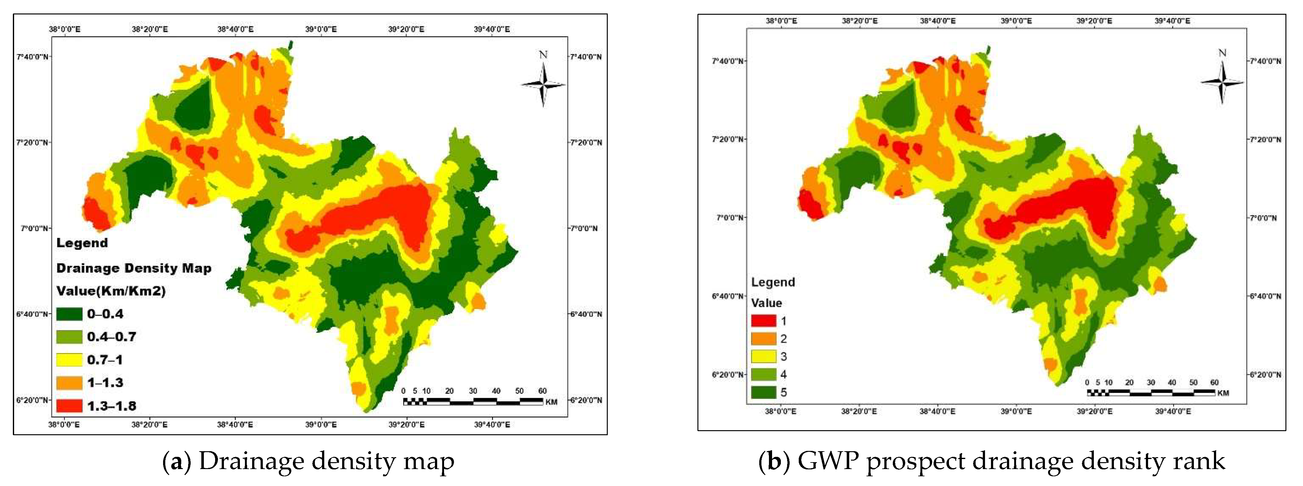
3.4. Drainage and Reclassified Drainage Density Layer

A drainage network is to a degree a panorama dissection with the aid of using streams and may be expressed as drainage density, indicating the entire length of streams associated with an area (km/km²) [57]. Drainage density has an inverse relation with the permeability of aquifers and performs an important position within the runoff distribution and degree of infiltration. Drainage density is one of the parameters affecting the groundwater potential, recharge, and play an essential position in groundwater potential zoning. Groundwater potential is poor in regions with a very excessive drainage density because it misplaces the majority in the form of runoff while regions with low drainage density permit extra infiltration to recharge the groundwater and, therefore, have extra for groundwater potential occurrence. According to [58], additionally cited, the low drainage density area has better infiltration and it yields higher groundwater potential zones, as compared to an excessive drainage density area. A dense drain is the consequence of feeble or impervious subsurface formations, light plant life, and mountainous relief. The drainage density of the looked at region starts from 0 to 1.8 km/km² (Figure 9a). About 46.32% of the place is predicted to have excessive to very excessive groundwater potential with respect to drainage density as shown in Table 12.

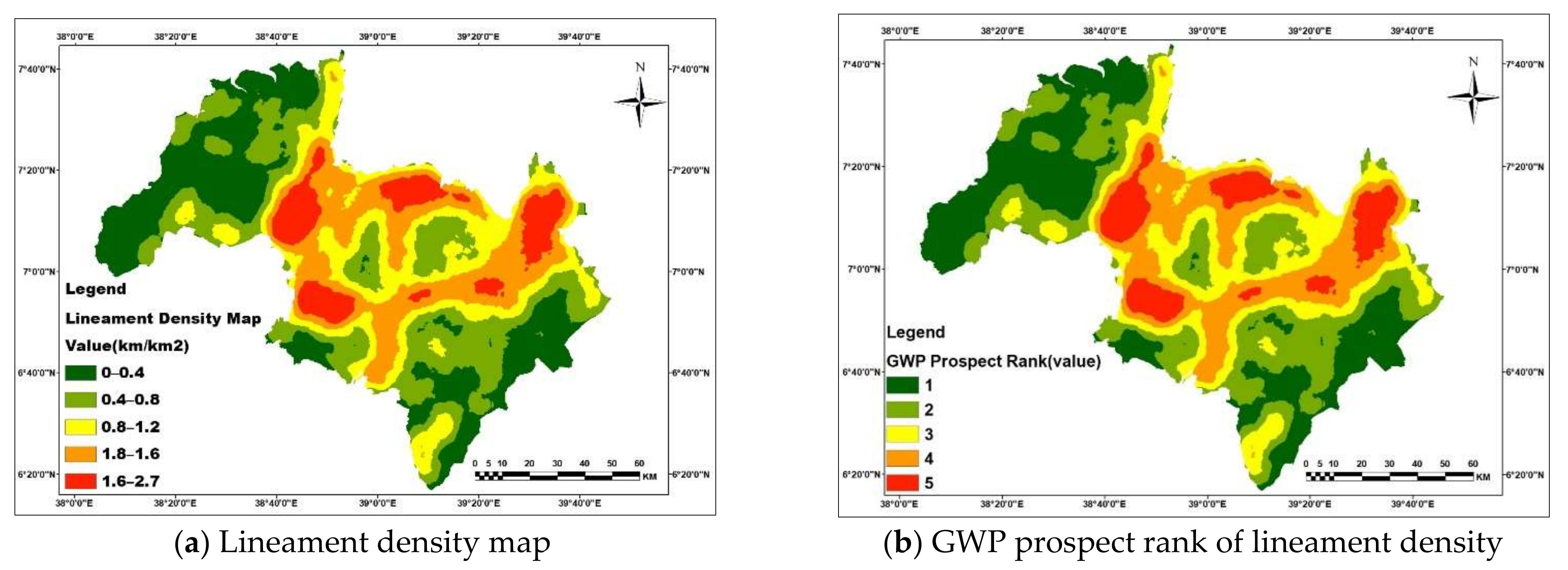
3.5. Lineament and Reclassified Lineament Density Layer

Geological formations that deliver rise to lineaments encompass faults, shear zones, fractures, dykes, and veins—in addition to bedding planes and stratigraphic contacts. The lineament density map shows the quantitative length of linear formations expressed in (km/km²). An excessive lineament length density suggests excessive secondary porosity, therefore representing a sector with excessive groundwater potential [59]. Lineament density is a crucial geological formation that have an effect on groundwater potential and recharge. Areas having a better lineament density facilitate infiltration and recharge of groundwater and, therefore, is proper for groundwater potential development. In turn, the ones having a low lineament density have low groundwater potential. Accordingly, only 27.94% of the place is predicted to have excessive to very excessive groundwater potential with respect to lineament density (Table 13).

3.6. LULC and Reclassified LULC Layer

The land-use and/or land-cover map is the principal issue for controlling the groundwater potential and recharge method. Its situations have an effect on the hydrologic cycle and hydrologic manner by changing the evapotranspiration, transpiration, infiltration, interception, and surface runoff, and thereby the groundwater potential distribution conduct in lots of ways. Due to population increase and different anthropogenic impacts in lots of watersheds, there is change in land use and/or land cover from one shape to the other [60,61,62,63]. Some land uses service the groundwater potential while others bring negative result to groundwater potential and recharge. Accuracy evaluation or validation is an essential step within the processing of remote sensing data, which determines the information value of the resulting data to a user [64]. The study had an average category accuracy of 87% and kappa coefficient (K) of 0.84. The kappa coefficient is rated as almost perfect and subsequently the classified image discovered to be a match for further research [27].

Built-up and rocky surfaces have much less opportunity of groundwater potential prevalence through growing runoff during rainfall while the surfaces protected through vegetation such as agricultural plants and forests have a better chance of groundwater opportunity due to higher infiltration through trapping and protecting the rainwater in roots of plants and cracks [65,66,67,68]. About 71.67% of a place is predicted to have excessive to very excessive groundwater potential with respect to land use/land cover (Table 14).

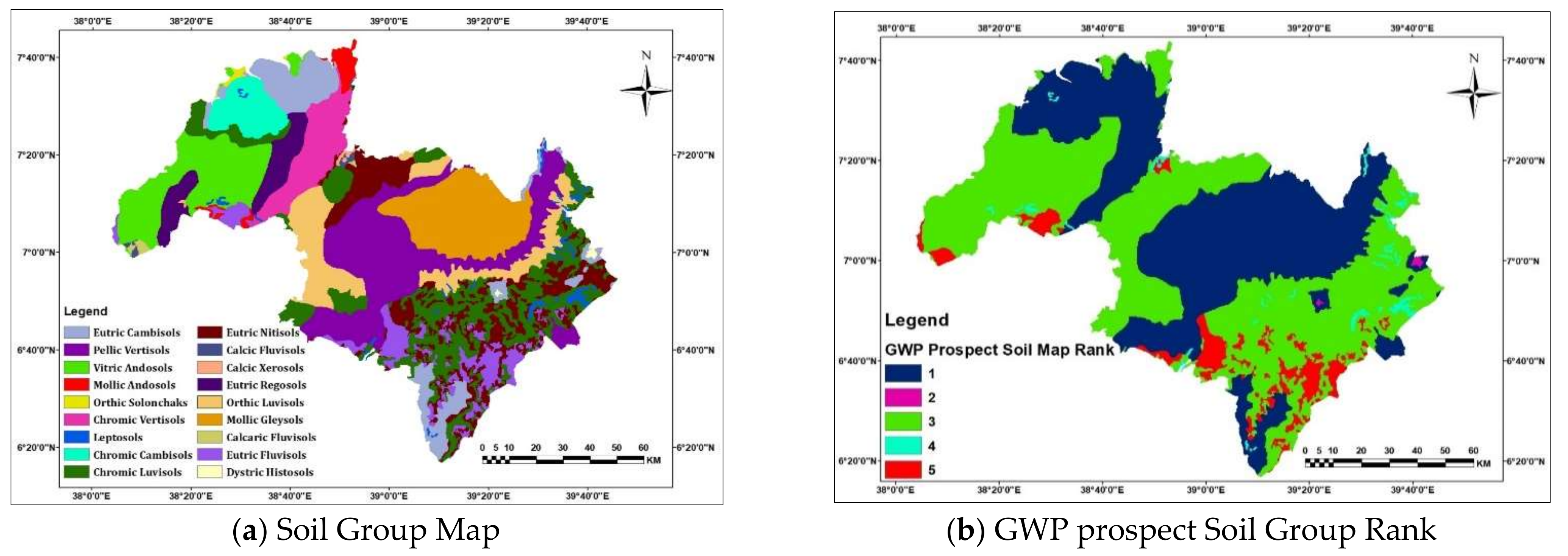
3.7. Soil and Reclassified Soil Group Layer

The water-conserving capability of a place relies upon the soil sorts and their permeability [69]. Soil mainly influences the rainfall infiltration and percolation strategies that, in the long run, impact the groundwater recharge after which the groundwater potential of a given area [70,71]. Soil properties influence the connection among runoff and infiltration rates, which, in turn, controls the degree of permeability that determines the groundwater potential [72]. The permeability of the soil sorts relies upon their texture.

Therefore, to identify the soil group permeability of the study area, a different soil group was categorized into six soil texture families with its permeability rate and classes. In the reclassification of the soil map, soil group according to its texture and permeability classes was grouped in to five classes according to is contribution for groundwater potential and recharge (Table 15). About 7.3% of the area is expected to have high to very high groundwater potential with respect to soil group.

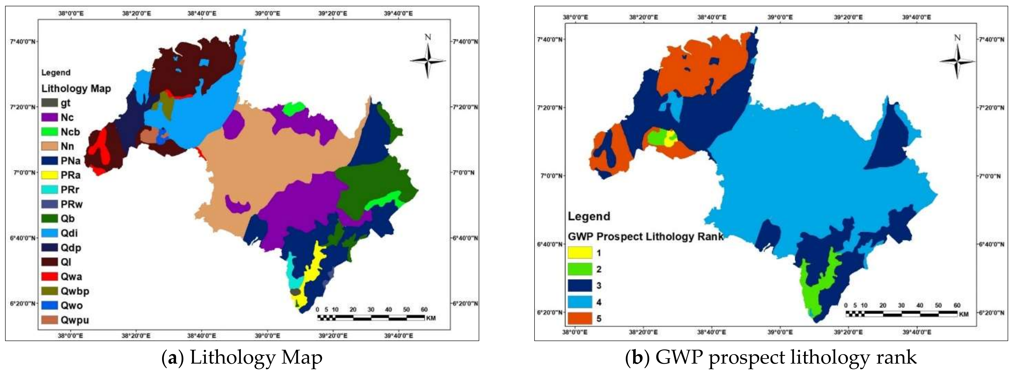
3.8. Lithology and Reclassified Lithology Layer

Geology or lithology is one of the groundwater potential and recharge controlling parameters taken into consideration in groundwater research, which plays a vital role in the distribution and prevalence of groundwater. Lithology is the bodily makeup of rocks and sediments and consists of mineral configuration, grain quartz, and grain packing [39]. Geology affects both the porosity and permeability of the aquifer material [1,73]. The Lithology of West Arsi area is grouped into distinctive kinds of formations/geological units [33,74,75,76,77,78,79]. However, every one of these lithological units do not have the same significance in determining and controlling groundwater potential and recharge. According to [74,75], the West Arsi lithological unit is categorized into 5 classes, depending on groundwater potential and recharge ability (Table 16). About 66.2% of the area is predicted to have excessive to very excessive groundwater potential with respect to the lithological units.

3.9. Weight Overlay Analysis

A main task within the proposed GIS-based multicriteria selection evaluation is the choice of criteria for groundwater potential area mapping wherein the criteria choice calls for suitable information of the site, the correct weighting of criteria through hydrogeologist experts, and correct cooperation among the decided-on factors. Pairwise comparison and Normalized Principal Eigen Vector (NPEV) found out that slope, LULC, and lithology are the most influential parameters, accounting for 24%. The percent weight of elevation, drainage density, lineament density, rainfall, and soil group is 9, 9, 5, 3, and 2, respectively (Table 6).

In computing the consistency ratio, the Principal Eigenvalue of 8.321 became done for an eight*eight matrix. Hence, the Principal Eigenvalue (λ_max) needs to constantly be greater than or identical to the number of the criteria (m) as in the above end result of λ_max, paving the way for the calculation of the consistency index (CI). Hence, pairwise comparison is reliable due to the fact the Principal Eigen value (λ_max), 8.321044984 calculated in Table 7, is greater than the number of criteria investigated (m), which was 8. Consistency index (CI) is 0.046.

The Random Index (RI) for the eight criteria is 1.41. The Consistency Ratio (CR) computed is 0.033, which is much less than 0.1 for large matrices more than 4 × 4 [38] and, therefore, the CR gained is suitable and the weight or percentage influence assigned for every thematic layer is acceptable.

3.10. Groundwater Potential Occurrence District Map

The groundwater potential sector was delineated with the aid of preparing maps, reclassifying, weighting, and ranking eight groundwater potential-influencing parameters (rainfall, lithology, slope, elevation, lineament density, drainage density, soil group, and LULC) in an ArcGIS environment applying weighted overlay analysis guided with AHP MCDM pairwise comparison techniques. The groundwater potential district layer was generated from superimposed thematic layers applying the weighted overlay approach with the help of spatial analysis tools in ArcGIS. In the weight overlay analysis and groundwater potential layer development, as found in

Table 17. Thematic maps rank and weight in terms of groundwater potential prospect.

Thematic Maps	Classes	Gw Prospect	Weight (%)	Rank
Rainfall	700.5–955.4	Very Low	3	1
	955.4–1210.8	Low		2
	1210.8–1466.2	Moderate		3
	1466.2–1721.6	High		4
	1721.6–1976.7	Very High		5
Soil Group	Eutric Cambisols/Pellic Vertisols/Orthic Solonchaks/Chromic Vertisols/Chromic Cambisols/Mollic Gleysols	Very Low	2	1
	Dystric Histosols	Low		2
	Vitric Andosols/Mollic Andosols/Chromic Luvisols/Eutric Nitisols/Eutric Regosols/Orthic Luvisols	Moderate		3
	Leptosols/Calcic Xerosols	High		4
	Calcic Fluvisols/Calcaric Fluvisols/Eutric Fluvisols	Very High		5
Lineament Density	0–0.4	Very Low	5	1
	0.4–0.8	Low		2
	0.8–1.2	Moderate		3
	1.2–1.6	High		4
	1.6–2.7	Very High		5
Lithology	Qwo	Very Low	24	1
	gt/PRa/PRr/Qwpu	Low		2
	PNa/PRw/Qdi/Qdp/Qwa	Moderate		3
	Nc/Ncb/Nn/Qb/Qwbp	High		4
	QI	Very High		5
LULC	Built Up Area	Very Low	24	1
	Barren Landscape	Low		2
	Forest	Moderate		3
	Agriculture & Vegetation	High		4
	Water Body	Very High		5
Slope	27.7–75.9	Very Low	24	1
	17.9–27.7	Low		2
	10.4–17.9	Moderate		3
	4.5–10.4	High		4
	0–4.5	Very High		5
Elevation/Altitude	3295–4171	Very Low	9	1
	2810–3295	Low		2
	2433–2810	Moderate		3
	1995–2433	High		4
	1464–1995	Very High		5
Drainage Density	1.3–1.8	Very Low	9	1
	1.0–1.3	Low		2
	0.7–1.0	Moderate		3
	0.4–0.7	High		4
	0–0.4	Very High		5

soil is assigned the lowest percentage of influence (weight), while slope, LULC, and lithology were assigned the higher weight/percentage influence. The spatial dispersal of groundwater potential and recharge throughout the study sector is the sum of the products of factors percentage influence (weight) and the corresponding reclassified parameters rank.

From

Table 18. West Arsi Zone groundwater potential distribution and its area coverage.

Value	GWP Prospect Rank	Count	Area (ha)	Area (%)
2	Low	109,176	9825.84	0.79
3	Moderate	4,896,961	440,726.49	35.46
4	High	8,460,429	761,438.61	61.27
5	Very High	341,652	30,748.68	2.47

above, about 61.27% of the area is anticipated to have high groundwater potential and 2.47% of the area is anticipated to have very high groundwater potential.

The reclassified thematic layers have a rank of 1 to 5, where 1 is very low, 2 low, 3 moderate, 4 high, and 5 very high groundwater prospects (Figure 5, Figure 6, Figure 7, Figure 8, Figure 9, Figure 10, Figure 11 and Figure 12). However, the weight overlay analysis produced ranks 2, 3, 4, and 5 only, which display the West Arsi region groundwater potential distribution being categorized into four classes: very high, high, moderate, and low (Figure 14a,b) groundwater potential and recharge zones. Figure 14c indicates regions of high groundwater potential are concentrated in the central and western a part of the study region, which covers an area of 61.27% (761,438.61 ha). Areas having very high groundwater potential is located at Shala, Arsi Negele, and the boundary of Shashemene and Siraro, which accounts about 2.47% (30,748.68 ha). The remaining part of the study region, 35.46% (440,726.49 ha), is classified as moderate groundwater potential in which the distribution is throughout the complete district; however, it is dominant on the eastern a part of the study location, and 0.79% (9825.84 ha) of the land is classified as low groundwater potential region, positioned in the Nensebo, Adeba, Shala, Siraro, Gedeb Asasa, and Shashemene Western and Southern sector of the study area in small amounts (Figure 14c).

In validating the groundwater potential distribution region layer, while the inventory data were plotted over the groundwater potential map (Figure 14d), from the 33 total number of wells categorized to low yield, 23 (69.70%) wells failed under the low groundwater potential region; from 69 total number of wells categorized to moderate yield, 67 (97.10%) wells failed under moderate groundwater potential; and from 11 total number of wells categorized to high yield, 9 (81.82%) wells failed under high groundwater potential region (

Table 19. Agreement (%) between the groundwater recharge zone map and borehole yield.

Groundwater Potential Zone Classes	Yield (L/s)	Total Number of Wells in Groundwater Potential Zone	Number of Wells Fall in Groundwater Potential Zone	Percent Agreement
Low	<2	33	23	69.70
Moderate	2–10	69	67	97.10
High and Very high	>10	11	9	81.82
Sum		113	99	87.61

). In cross validation evaluation from 113 borehole yields, 99 (87.61%) conform to the corresponding groundwater potential region classifications from the qualitative evaluation.

The validation results, 87.61% or 0.876, confirm that there may be a very good agreement among the groundwater inventory data and groundwater potential zones delineated applying GIS and RS techniques. Therefore, the results of the groundwater potential maps obtained with the support of the AHP technique and weight overlay analysis were taken into consideration as a very good prediction. This indicates that the findings developed from the study are proper compared with the well yield of the point inventory acquired from the field.

4. Conclusions

Increased availability of remotely sensed information has helped in analyzing the natural surroundings without direct measuring in field. Remote Sensing (RS) and Geographic Information System (GIS) are possible in terms of cost, time, and resources, which make it fast, correct, and economical strategies to be utilized in groundwater potential and recharge sector evaluation than the traditional ground survey and resistivity methods. It incorporates comparing groundwater potential zones of the study area by applying the different groundwater spatial parameters.

The occurrence and distribution of groundwater potential specifically relies upon on the groundwater potential-affecting parameters. The most vital parameters affecting groundwater potential and the recharge sector decided on for this study were rainfall, lithology/geology, lineament density, LULC, soil group and texture, slope, elevation/altitude/geomorphology, and drainage density. Therefore, assessment of the groundwater potential sector of a place was carried out via way of means of analysis of those parameters. Those parameter factors were reclassified and ranked according to its significance in influencing groundwater potential.

Weighted value or percent influence determination was done with the reclassified thematic prepared and the organized maps. Weighted value or percentage influence dedication were completed with reclassified thematic organized and prepared maps. Weight overlay analysis considers all parameters that have an impact on groundwater potential; it offers the correct weight for parameters; it offers ranking of the characteristics of the parameters and exercising through the cell. Therefore, it better estimated the groundwater potential distribution throughout the region. Groundwater potential and recharge district affecting parameters taken into consideration in this study do not have a similar influence on groundwater potential distribution and the recharge zone. The percent influence (weight) of those parameters was decided applying Analytic Hierarchy Process (AHP) Multi-Criteria Decision Making (MCDM) pairwise comparison matrix techniques.

Weight overlay analysis produced 24% for slope, lithology, and LULC; 9% for elevation; 9% for drainage density; 5% for lineament density; 3% for rainfall; and 2% for soil group. Accordingly, slope, LULC, and lithology were found the most significant parameters. Whereas, lineament density, rainfall, and soil group were the least groundwater potential-influencing parameters.

Groundwater distribution throughout the West Arsi Zone is not uniform according to this study and therefore classified into very high (2.47%, which is 30,748.68 ha), high (61.27%, which is 761,438.61 ha), moderate (35.46%, which is 440,726.49 ha), and low (0.79%, which is 9825.84 ha) groundwater potential distribution.

The suitable groundwater potential and recharge areas are found with lithological formation of QI (lacustrine sediments deposits, silt clays, diatomite, and minor ignimbrites), Qwbp (Pleistocene basalt), Qb (alkaline basalt and trachyte), Nn (ignimbrite, un-welded tuffs, ash flows, rhyolites, domes, and trachyte), Ncb (alkaline basalts and trachyte), and Nc (basalt and peralkaline rhyolite with minor alkaline basalt). LULC areas covered with a water body, agricultural practices, and area covered with vegetation are suitable for groundwater potential formation. Areas acquired excessive annual common rainfall were given excessive groundwater potential. A location with a low slope, elevation, and drainage density are good for groundwater potential and recharge. In turn, locations with excessive lineament density were discovered to be the most essential regarding groundwater potential and recharge. Soil groups of leptosols, calcic xerosols, calcic fluvisols, calcaric fluvisols, and eutric fluvisols, and those with a sandy loam and loamy sand texture, permit infiltration and percolation, which will increase groundwater potential and recharge.

The groundwater potential distribution assessed and the map generated were validated using borehole inventory data. Accordingly, the percent agreement between the groundwater potential recharge zone map generated and inventory borehole yield found in the rank analysis was 87.61%, which is in very good agreement.

References

- Chowdhury, J.; Jhan, M.K.; Chowdary, V.M.; Mal, B.C. Integrated Remote Sensing and GIS Based Approach for Assessing Groundwater Potential in West Mendinipur district, West Bengal, India. Int. J. Remote Sens. 2010, 30, 231–250. [Google Scholar] [CrossRef]
- Jhan, M.; Chowdary, V.; Chowdhury, A. Groundwater Assessment in Salboni Block, West Bengal, India Using Remote Sensing, Geographic Information System and Multi-criteria Decision Analysis Techniques. Hydrogeol. J. 2012, 18, 1713–1728. [Google Scholar] [CrossRef]
- Naghibi, S.A.; Moradi, D.M. Evaluation of four supervised learning methods for groundwater spring potential mapping in Khalkhal region, Iran, using GiS- based features. Hydrogeol. J. 2017, 25, 169–189. [Google Scholar] [CrossRef]
- Naghibi, S.A.; Moghaddam, D.D.; Kalantar, B.; Pradhan, B.; Kisi, O. A comparative assessment of GIS-based data mining models and a novel ensemble model in groundwater well potential mapping. J. Hydrol. 2017, 548, 471–483. [Google Scholar] [CrossRef]
- Maniar, H.H.; Bhatt, N.J.; Prakash, I.; Mahmood, K. Application of Analytical Hierarchy Process (AHP) and GIS in the Evaluation of Groundwater Recharge Potential of Rajkot District, Gujarat, India. Int. J. Tech. Innov. Mod. Eng. Sci. 2017, 5, 1078–1087. [Google Scholar]
- Zeinolabedini, M.; Esmaeili, A. Groundwater Potential Assessment Using Geographic Information Systems and AHP Method (Case Study: Baft City, Kerman, Iran). Int. Arch. Photogramm. Remote Sens. Spat. Inf. Sci. 2015, 1, W5. [Google Scholar] [CrossRef] [Green Version]
- Krishnamurthy, J.; Mani, A.; Jayaraman, V.; Manivel, M. Groundwater resources development in hard rock terrain: An approach using remote sensing and GIS techniques. Int. J. Appl. Earth Obs. Geoinf. 2000, 3, 204–215. [Google Scholar] [CrossRef]
- Saraf, A.K.; Choudhury, P.R. Integrated remote sensing and GIS for groundwater exploration and identification of artificial recharge sites. Int. J. Remote Sens. 1998, 19, 1825–1841. [Google Scholar] [CrossRef]
- Carver, S. Integrating multi-criteria evaluation with geographic information systems. Int. J. Geogr. Inf. Syst. 1991, 5, 321–339. [Google Scholar] [CrossRef] [Green Version]
- Bahunguna, I.M.; Nayak, S.; Tamilarsan, V.; Moses, J. Groundwater prospective zones in basaltic terrain using remote sensing. J. Indian Soc. Remote Sens. 2003, 31, 101–105. [Google Scholar] [CrossRef]
- Das, S.; Behera, S.C.; Kar, A.; Narendra, P.; Guha, S. Hydro geomorphological mapping in groundwater exploration using remotely sensed data: Case study in Keonjhar district, Orissa. J. Indian Soc. Remote Sens. 1997, 25, 245–259. [Google Scholar] [CrossRef]
- Das, S.; Pardeshi, S.D. Integration of different influencing factors in GIS to delineate groundwater potential areas using IF and FR techniques: A study of Pravara basin, Maharashtra, India. Appl. Water Sci. 2018, 8, 197. [Google Scholar] [CrossRef] [Green Version]
- Dar, I.A.; Sankar, K.; Dar, M.A. Remote sensing technology and geographic information system modeling: An integrated approach towards the mapping of potential groundwater recharge zones in hard rock terrain, Mamundiyar basin. J. Hydrol. 2010, 394, 285–295. [Google Scholar] [CrossRef]
- Singh, P.; Thakur, J.K.; Kumar, S. Delineating groundwater potential zones in a hard-rock terrain using geospatial tool. Hydrol. Sci. J. 2013, 58, 213–223. [Google Scholar] [CrossRef] [Green Version]
- Saaty, T. Decision making with the analytic hierarchy ptocess. Int. J. Serv. Sci. 2008, 1, 83–89. [Google Scholar]
- Doke, A.B.; Zolekar, R.B.; Patel, H.; Das, S. Geospatial mapping of groundwater potential zones using multi-criteria decision-making AHP approach in a hardrock basaltic terrain in India. Ecol. Indic. 2021, 127, 107685. [Google Scholar] [CrossRef]
- Sresto, M.A.; Siddika, S.; Haque, M.N.; Saroar, M. Application of fuzzy analytic hierarchy process and geospatial technology to identify groundwater potential zones in north-west region of Bangladesh. Environ. Chall. 2021, 5, 100214. [Google Scholar] [CrossRef]
- Karimi-Rizvandi, S.A.; Goodarzi, H.V.; Afkoueieh, J.H.; Chung, I.-M.; Kisi, O.; Kim, S.; Linh, N.T.T. Groundwater-Potential Mapping Using a Self-Learning Bayesian Network Model: A Comparison among Metaheuristic Algorithms. Water 2021, 13, 658. [Google Scholar] [CrossRef]
- Maity, B.; Mallick, S.K.; Das, P.; Rudra1, S. Comparative analysis of groundwater potentiality zone using fuzzy AHP, frequency ratio and Bayesian weights of evidence methods. Appl. Water Sci. 2022, 12, 63. [Google Scholar] [CrossRef]
- Tamiru, H.; Wagari, M. Comparison of ANN model and GIS tools for delineation of groundwater potential zones, Fincha Catchment, Abay Basin, Ethiopia. Geocarto Int. 2021, 1–19. [Google Scholar] [CrossRef]
- Nguyen, P.T.; Ha, D.H.; Jaafari, A.; Nguyen, H.D.; van Phong, T.; Al-Ansari, N.; Prakash, I.; van Le, H.; Pham, B.T. Groundwater Potential Mapping Combining Artificial Neural Network and Real AdaBoost Ensemble Technique: The DakNong Province Case study, Vietnam. Int. J. Environ. Res. Public Health 2020, 17, 2473. [Google Scholar] [CrossRef] [Green Version]
- Razavi-Termeh, S.V.; Sadeghi-Niaraki, A.; Choi, S.-M. Groundwater Potential Mapping Using an Integrated Ensemble of Three Bivariate Statistical Models with Random Forest and Logistic Model Tree Models. Water 2019, 11, 1596. [Google Scholar] [CrossRef] [Green Version]
- Mallick, J.; Khan, R.A.; Ahmed, M.; Alqadhi, S.D.; Alsubih, M.; Falqi, I.; Hasan, M.A. Modeling Groundwater Potential Zone in a Semi-Arid Region of Aseer Using Fuzzy-AHP and Geoinformation Techniques. Water 2019, 11, 2656. [Google Scholar] [CrossRef] [Green Version]
- Farzin, M.; Avand, M.; Ahmadzadeh, H.; Zelenakova, M.; Tiefenbacher, J.P. Assessment of Ensemble Models for Groundwater Potential Modeling and Prediction in a Karst Watershed. Water 2021, 13, 2540. [Google Scholar] [CrossRef]
- Congalton, R. A review of assessing the Accuracy of classifications of remotely sensed data. Remote Sens. Environ. 1991, 37, 35–46. [Google Scholar] [CrossRef]
- Jensen, J. Introductory Digital Image Processing: A Remote Sensing Perspective, 2nd ed.; Prentice Hall, Inc.: Upper Suddle River, NJ, USA, 1996. [Google Scholar]
- Rwanga, S.S.; Ndambuki, J.M. Accuracy Assessment of land use land cover classification using remote sensing and GIS. Int. J. Geosci. 2017, 8, 611–622. [Google Scholar] [CrossRef] [Green Version]
- ESRI. ArcGIS Desktop: Release 10.3.1; Environmental Systems Research in USA: Redlands, CA, USA, 2015. [Google Scholar]
- Singh, P.; Gupta, A.; Singh, M. Hydrological Inferences from watershed analysis for water resource management using remote sensing and GIS techniques, Egypt. J. Remote Sens. Space Sci. 2014, 17, 111–121. [Google Scholar]
- Rusli, N.; Majid, M.R. Digital Elevation Model (DEM) Extraction from Google Earth: A Study in Sungai Muar Watershed; Applied Geoinformatics for Society and Environment: Garching bei München, Germany, 2012; pp. 32–36. ISBN 978-3-943321-06-7. [Google Scholar]
- Hobbs, W. Lineaments of the Atlantic border region. Geol. Soc. Am. Bull. 1904, 15, 483–506. [Google Scholar] [CrossRef]
- Clark, C.D.; Wilson, C. Spatial Analysis of Lineaments. Comput. Geosci. 1994, 20, 1237–1258. [Google Scholar] [CrossRef]
- GSE. Geological Map of Oromia; Ethiopian Mapping Authority: Addis Ababa, Ethiopia, 1999. [Google Scholar]
- Yeh, H.F.; Cheng, Y.S.; Lin, H.I.; Lee, C.H. Mapping groundwater recharge potential zone using a GIS approach in Hualian River, Taiwan. Sust. Environ. Res. 2016, 26, 33–43. [Google Scholar] [CrossRef] [Green Version]
- Hussein, A.A.; Govindu, V.; Nigusse, A.G.M. Evaluation of Groundwater potential using geospatial techniques. Appl. Water Sci. 2017, 7, 244–246. [Google Scholar] [CrossRef] [Green Version]
- Singh, L.K.; Jha, M.K.; Chowdary, V.M. Multi-criteria analysis and GIS modeling for identifying prospective water harvesting and artificial recharge sites for sustainable water supply. J. Clean. Prod. 2017, 142, 1436–1456. [Google Scholar] [CrossRef]
- Saaty, T.L. The Analytical Hierarchy Process; WS Publication: Manila, PH, USA, 1990; ISBN1 0962031720. ISBN2 9780962031724. [Google Scholar]
- Saaty, T.L. Decision Making for Leaders; RWS Publications: Pittsburgh, PA, USA, 1995. [Google Scholar]
- Freeze, R.A.; Cherry, J.A. Groundwater; Prentice-Hall, Inc.: Hoboken, NJ, USA, 1979. [Google Scholar]
- Abdel Rahman, R. A Modified Analytical Hierarchy Process Method to Select Sites for Groundwater Recharge in Jordan. Ph.D. Dissertation, University of Leicester, Leicester, UK, 2015. [Google Scholar]
- Kotchoni, D.O.V.; Vouillamoz, J.; Lawson, F.M.A. Relationship between rainfall and groundwater recharge in seasonal humid Benin: A comparative analysis of long-term hydrographs in sedimentary and crystalline aquifers. Hydrogeol. J. 2019, 27, 447–457. [Google Scholar] [CrossRef] [Green Version]
- Ramu, M.; Vinay, M. Identification of groundwater potential zones using GIS and remote sensing techniques: A case study of Mysore taluk Karnataka. Int. J. Geomat. Geosci. 2015, 5, 393–403. [Google Scholar]
- Zomlot, Z.; Verbeiren, B.; Huysmans, M.; Batelaan, O. Spatial distribution of groundwater recharge and base flow: Assessment of controlling factors. J. Hydrol. Reg. Stud. 2015, 4, 349–368. [Google Scholar]
- Shakya, B.M.; Nakamura, T.; Shrestha, S.D.; Nishida, K. Identifying the deep groundwater recharge Processes in an intermountain basin using the hydrogeochemical and water isotope characteristics. Nord. Hydrol. 2019, 50, 1216–1229. [Google Scholar] [CrossRef] [Green Version]
- Wang, J.; Huo, A.; Zhang, X. Prediction of the response of groundwater recharge to climate changes in Heihe river basin, China. Environ. Earth Sci. 2020, 79, 1–16. [Google Scholar] [CrossRef]
- Dabrala, S.; Bhatt, B.; Joshi, J.P.; Sharma, N. Groundwater Suitability recharge zones modelling: A GIS application. ISPRS 2014, 8, 347–352. [Google Scholar] [CrossRef] [Green Version]
- Saaty, T. Decision making with the AHP: Why is the principal eigenvector necessary. Eur. J. Oper. Res 2003, 145, 85–91. [Google Scholar] [CrossRef]
- Brunelli, M. Introduction to the Analytic Hierarchy Process; Springer: New York, NY, USA, 2015; p. 83. ISBN 978-3-319-12501-5. [Google Scholar] [CrossRef] [Green Version]
- Saaty, T. The Analytic Hierarchy Process (AHP) for Decision Making. In Kobe, Japan. 1980, pp. 1–69. Available online: http://www.cashflow88.com/decisiones/saaty1.pdf (accessed on 5 May 2022).
- Senanayake, I.P.; Dissanayake, D.M.; Mayadunna, B.B.; Weerasekera, W.L. An Approach to delineate groundwater recharge potential sites in Ambalantota, Sri Lanka using GIS techniques. Geosci. Front. 2016, 7, 115–124. [Google Scholar] [CrossRef] [Green Version]
- Sahoo, S.; Jha, M.K.; Kumar, N.; Chowdary, V.M. Evaluation of GIS based Multicriteria decision analysis and probabilistic modeling for exploring groundwater prospects. Environ. Earth Sci. 2015, 74, 2223–2246. [Google Scholar]
- Yesilnacar, E.; Topal, T. Landslide susceptibility mapping: A comparison of logistic regression and natural networks methods in a medium scale study, Hendek region (Turkey). Eng. Geol. 2005, 79, 251–266. [Google Scholar] [CrossRef]
- Lerner, D.N.; Issar, A.S.; Simmers, I. Groundwater Recharge: A Guide to Understanding and Estimating Natural Recharge; IAH International Contributions to Hydrogeology, 8; Taylor and Francis: Rotterdam, The Netherlands, 1990. [Google Scholar]
- Andualem, T.G.; Demeke, G.G. Groundwater potential assessment using GIS and Remote sensing: Study of guna Tana landscape, Upper Blue Nile basin, Ethiopia. J. Hydrol. Reg. Stud. 2019, 24, 3. [Google Scholar] [CrossRef]
- Dufy, C.J.; Al-Hassan, S. Groundwater circulation in a closed desert basin: Topographic scaling and climatic forcing. Water Resour. Res. 1988, 24, 1675–1688. [Google Scholar] [CrossRef]
- Todd, D.K.; Mays, L.W. Groundwater Hydrology, 3rd ed.; John Wiley & Sons, Inc.: New York, NY, USA, 2005. [Google Scholar]
- Schillaci, C.; Braun, A.; Kropacek, J. Terrain Analysis and Landform Recognition. In Geomorphological Techniques; British Society for Geomorphology: London, UK, 2015; Chapter 2. [Google Scholar]
- Murasingh, S. Analysis of Groundwater Potential Zones Using Electrical Resistivity: Remote Sensing and GIS Techniques in a Typical Mine Area of Odisha; National Institute of Technology: Rourkela, India, 2014. [Google Scholar]
- Al-Abadi, A.M.; Al-Shamma, A. Groundwater potential mapping of the major aquifer in Northeastern Missan Governorate, South of Iraq by using AHP and GIS. J. Environ. Earth Sci. 2014, 10, 125–149. [Google Scholar]
- Kenji, J.; Atsushi, T.; Othoman, A.; Susumu, S.; Ronny, B. Effects of land use change on groundwater recharge model parameters. Hydrol. Sci. J. Des. Sci. Hydrol. 2009, 54, 300–315. [Google Scholar] [CrossRef]
- Pan, Y.; Gong, H.; Zhou, D.; Li, X.; Nakagoshi, N. Impact of land use change on groundwater recharge in Guishui river basin, China. Chin. Geogr. Sci. 2011, 21, 734–743. [Google Scholar] [CrossRef]
- Owuor, S.O.; Butterbach-Bahl, K.; Guzha, A.C.; Rufino, M.C.; Pelster, D.E.; Díaz-Pinés, E.; Breuer, L. Groundwater recharge rates and surface runoff response to land use and land cover changes in semi-arid environments. Ecol. Processes 2016, 5, 16. [Google Scholar] [CrossRef] [Green Version]
- Riley, D.; Mieno, T.; Schoengold, K.; Brozović, N. The impact of landcover on groundwater recharge in the high plains: An application to the conservation reserve program. Sci. Total Environ. 2019, 696, 133871. [Google Scholar] [CrossRef]
- Abubaker, H.M.; Elhag, A.M.H.; Salih, A.M. Accuracy assessment of land use land cover classification: Case study of Shomadi area-Renk county, upper Nile State, South Sudan. Int. J. Sci. Res. Publ. 2013, 3, 2250–3153. Available online: http://citeseerx.ist.psu.edu/viewdoc/summary?doi=10.1.1.414.8771 (accessed on 5 May 2022).
- Shaban, A.; Khawlie, M.; Abdallah, C. Use of remote sensing and GIS to determine recharge potential zone: The case of Occidental, Lebanon. Hydrogeol. J. 2006, 14, 433–443. [Google Scholar] [CrossRef]
- Singh Sk Singh, C.K.; Mukherjee, S. Impact of land use and land cover change on groundwater quality in the lower Shiwalik hills: A remote sensing and GIS based approach. Cent. Eur. J. Geosci. 2010, 2, 124–131. [Google Scholar] [CrossRef]
- Fenta, A.A.; Kife, A.; Gebreyohannes, T.; Hailu, G. Spatial analysis of groundwater potential using remote sensing and GIS based multi-criteria evaluation in Raya Valley, northern Ethiopia. Hydrogeol. J. 2015, 23, 195–206. [Google Scholar] [CrossRef]
- Li, S.; Yang, H.; Lacayo, M.; Liu, J.; Lei, G. Impacts of land use and land cover changes on water yield: A case study in Jing-jin-ji., China. Sustainability 2018, 10, 960. [Google Scholar] [CrossRef] [Green Version]
- Kumar, P.; Herath, S.; Avtar, R.; Takeuchi, K. Mapping of groundwater potential zones in Killinochi area, Sri Lanka, using GIS and remote sensing techniques. Sustain. Water Resour. Manag. 2016, 2, 419–430. [Google Scholar] [CrossRef] [Green Version]
- Anuraga, T.S.; Ruiz, L.; Mohan Kumar, M.S.; Sekhar, M.; Leijnse, A. Estimating groundwater recharge using land use and soil data: A case study in south india. Agric. Water Manege. 2006, 84, 65–76. [Google Scholar] [CrossRef]
- Rukundo, E.; Dogan, A. Dominant influencing factors of groundwater recharge spatial patterns in Ergene river catchment, Turkey. Water 2019, 11, 653. [Google Scholar] [CrossRef] [Green Version]
- Tesfaye, T. Ground Water Potential Evaluation Based on Integrated GIS and Remote Sensing Techniques, in Bilate River Catchment: South Rift Valley of Ethiopia. Am. Acad. Sci. Res. J. Eng. Technol. Sci. 2014, 10, 85–120. [Google Scholar]
- Yazi, A.; Pirasteh, S.; Arvin, A.; Pradhan, B.; Nikouravan, B.; Mansor, S. Dsasters and Risk reduction in Groundwater: Zagros Mountain southwest Iran using geoinformatics techniques. Interdiscip. Neurosurg. 2010, 3, 51–57. [Google Scholar]
- GSE. Integrated Hydrological and Hadrochemical Mapping of Yiag Map Sheet. 2003. Available online: https://gis.gse.gov.et/hg-maps/ (accessed on 15 April 2020).
- Halcrow, G. Rift Valley Lakes Basin Integrated Resources Development Master Plan Study Project; Draft Phase 2 Report Part II Prefeasibility Studies; Unpublished Report; Halcrow Group Limited: London, UK; GIRD Consultants: Mumbai, India, 2008. [Google Scholar]
- Kefale, T.; Jiri, S. Hydrogeological and Hydro Chemical Maps of Hosaina Explanatory Notes (NB 37-2); Antonin Orgon: Prague, Czech Republic, 2013. [Google Scholar]
- Astatike, K.; Sima, J. Hydrogeological and Hydro Chemical Maps of Asela Explanatory Notes (NB37-3); Antonin Orgon: Prague, Czech Republic, 2012. [Google Scholar]
- Astatike, K.; Sima, J. Hydrogeological and Hydro Chemical Maps of Dodola Explanatory Notes (NB 37-7); Antonin Orgon: Prague, Czech Republic, 2011. [Google Scholar]
- Thomas, A.; Tegist, R.; Sima, J. Hydrogeological and Hydro Chemical Maps of Dila Explanatory Notes (NB 37-6); Antonin Orgon: Prague, Czech Republic, 2014. [Google Scholar]
Figure 1.
Location map of West Arsi Zone.
Figure 2.
Three river basins drain the West Arsi Zone and West Arsi districts.
Figure 3.
Research methodology flowchart.
Figure 4.
(a) Random points plot on the LULC map. (b) Random points plotted on Google Earth Pro in kml format.
Figure 5.
LULC and groundwater potential prospect rank of the LULC map.
Figure 6.
Rainfall and groundwater potential prospect rank of the rainfall map.
Figure 7.
Slope and groundwater potential prospect rank of the slope map.
Figure 8.
Elevation and groundwater potential prospect rank of the elevation map.
Figure 9.
Drainage density and groundwater potential prospect rank of the drainage density map.
Figure 10.
Lineament density and groundwater potential prospect rank of the lineament density map.
Figure 11.
Soil group and groundwater potential prospect rank of the soil group map.
Figure 12.
Lithology and groundwater potential prospect rank of the lithology map.
Figure 13.
AHP Procedure to determine and validate the percent weight (NPEV).
Figure 14.
Groundwater potential map and well yield plot over it for validation.