
Multi-Variables-Driven Model Based on Random Forest and Gaussian Process Regression for Monthly Streamflow Forecasting


1
Faculty of Automation, Huaiyin Institute of Technology, Huaian 223003, China
2
Key Laboratory of Thermo-Fluid Science and Engineering, Ministry of Education, School of Energy & Power Engineering, Xian Jiaotong University, Xi’an 710049, China
3
School of civil and hydraulic engineering, Huazhong University of Science and Technology, Wuhan 430074, China
4
Water Resources Research Center, China Yangtze Power Co., Ltd., Yichang 443002, China
*
Author to whom correspondence should be addressed.
Water 2022, 14(11), 1828; https://doi.org/10.3390/w14111828
Submission received: 13 April 2022
/
Revised: 1 June 2022
/
Accepted: 3 June 2022
/
Published: 6 June 2022
(This article belongs to the Section Hydrology)
Abstract
:Due to the inherent non-stationary and nonlinear characteristics of original streamflow and the complicated relationship between multi-scale predictors and streamflow, accurate and reliable monthly streamflow forecasting is quite difficult. In this paper, a multi-scale-variables-driven streamflow forecasting (MVDSF) framework was proposed to improve the runoff forecasting accuracy and provide more information for decision-making. This framework was realized by integrating random forest (RF) and Gaussian process regression (GPR) with multi-scale variables (hydrometeorological and climate predictors) as inputs and is referred to as RF-GPR-MV. To validate the effectiveness and superiority of the RF-GPR-MV model, it was implemented for multi-step-ahead monthly streamflow forecasts with horizons of 1 to 12 months for two key hydrological stations in the Jinsha River basin, Southwest China. Other MVDSF models based on the Pearson correlation coefficient (PCC) and GPR with/without multi-scale variables or the PCC and a backpropagation neural network (BP) or general regression neural network (GRNN), with only previous streamflow and precipitation, namely, PCC-GPR-MV, PCC-GPR-QP, PCC-BP-QP, and PCC-GRNN-QP, respectively, were selected as benchmarks. Experimental results indicated that the proposed model was superior to the other benchmark models in terms of the Nash–Sutcliffe efficiency (NSE) for almost all forecasting scenarios, especially for forecasting with longer lead times. Additionally, the results also confirmed that the addition of large-scale climate and circulation factors was beneficial for promoting the streamflow forecasting ability, with an average contribution rate of about 15%. The RF in the MVDSF framework improved the forecasting performance, with an average contribution rate of about 25%. This improvement was more pronounced when the lead time exceeded 3 months. Moreover, the proposed model could also provide prediction intervals (PIs) to characterize forecast uncertainty, as supplementary information to further help decision makers in relevant departments to avoid risks in water resources management.
1. Introduction
Accurate and reliable streamflow forecasting is an important basis for rational allocation and sustainable utilization of water resources [1,2]. It can not only provide key decision-making information for avoiding natural disasters such as floods and droughts but also be conducive to the safe and economic operation of reservoirs and the coordination of water utilization among different departments in order to realize the most comprehensive benefits [3]. As is well known, the evolution of a water cycle system is affected by the synthetical effects of weather, the underlying surface, the ocean, and climate. Such a complex water cycle system will produce streamflow with many natural characteristics such as high-dimensional nonlinearity, non-stationarity, wet and dry alternation, and uneven spatial and temporal distribution. These inherent features make it difficult to predict streamflow accurately, especially in a changing environment.
Most historical studies focused on studying new streamflow forecasting models to adapt to the changing world. The forecasting models can be roughly divided into two main classes: physical models (PMs) and data-driven models (DDMs) [4]. Models in the first group use a series of mathematical and physical equations to represent evaporation, interception, infiltration, and other key processes of a water cycle system. Hence, PMs always have high demands in many areas, requiring, e.g., a deep understanding of the physical mechanisms of hydrological processes, large amounts of input climate data, large numbers of parameters to be estimated, large computational resources, and so on. Therefore, they are rarely used in practice.
Unlike PMs, DDMs have simpler model structures and need less modeling data. Early DDMs mainly focused on regression models such as linear regression models, autoregressive models, autoregressive moving average (ARMA) models, autoregressive integrated moving average models, moving average models, and so on [5]. Due to the nonlinearities and uncertainties of streamflow, existing regression methods often do not provide the desired forecasting accuracy. Nowadays, with the development of machine learning (ML) techniques, DDMs have attracted much more attention as an alternative forecasting tool for monthly streamflow. To date, a number of DDMs based on ML techniques have been utilized successfully for streamflow forecasting. For example, ANNs (artificial neural networks) are widely used to describe hydrological behavior and have a good nonlinear fitting performance in comparison to traditional regression models [6]. Support vector machine (SVM) and least squares support vector machine (LSSVM) models are also employed in streamflow forecasting, and show good performances [7,8]. Evolutionary adaptive neuro-fuzzy inference systems (ANFIS) [9,10], extreme learning machine (ELM) [4,11,12] and random forest (RF) [13,14] models have also shown potential for streamflow forecasting. Recently, deep learning techniques such as convolutional neural networks (CNNs) [15], long short-term memory networks (LSTMs) [16,17] and their associated variants, gated recurrent units (GRU) [18], stacked LSTMs (S-LSTMs), and bidirectional LSTMs (Bi-LSTMs) [19] have been popular in hydrology forecasting. However, pure ML models still provide poor forecasting accuracy for complex nonlinear and non-stationary runoff series when the model is developed with only previous rainfall information as input [20].
To further promote the performance of a DDM based on machine learning, two methods are often utilized. The first approach is to consider more climate factors as inputs rather than just rainfall information [21,22,23,24]. In this case, the more factors that are considered, the more complex the prediction model will be. Thus, an efficient input variable selection (IVS) method must be used. Unfortunately, there are no general methods available at present. Widely used IVS techniques can be divided into wrapper (also called model-based) and filter (also called model-free) methods [25,26]. The wrapper method depends on the idea of training and testing several forecasting models with different input sets and determining the optimal input set with the best model performance. Unlike the wrapper approach, filter approaches directly determine the optimal input vector according to some index relating the candidate input vector and the forecasted variable (such as distance between classes, statistical correlation, or information theory). Representative and widely used filter approaches include Pearson correlation coefficient (PCC) [27,28] and partial mutual information (PMI) [26] methods. Usually, wrapper approaches achieve better performances, but they have higher computational resource requirements than filter methods. In this paper, a wrapper method is applied to determine the optimal predictors, to take advantage of the easy hybridization of machine learning techniques. In this paper, two types of IVS are adopted. One is a filter method named PCC, which is well-known for its simple operation. The other is random forest (RF), a typical ML method with the advantage over other commonly used ANNs and SVMs of needing no optimization [29]. In most previous applications of RF in hydrological prediction, it has been used as a prediction model rather than an IVS method. Pham et al. [30] evaluated the potential of RF to achieve streamflow forecasts. Shen et al. [31] used RF for correcting daily discharge predictions. Ahana et al. [32] examined the abilities of LSTM, ELM, and RF to predict monthly streamflow. This paper focuses on the utilization of the ability of RF for feature selection.
Another way to improve the performance of DDM forecasting models is by using hybrid models, which integrate signal decomposition algorithms and/or optimization algorithms. For example, Yaseen et al. [33] applied three different bio-inspired optimization algorithms (GA, PSO, and DE) to optimize the membership function of ANFIS. Chen et al. [4] used BSA to optimize the parameters of the standard ELM model, to improve flood forecasting accuracy. Maheswaran and Khosa [34] proposed a wavelet–Volterra coupled (WVC) model for one-month-ahead streamflow forecasting. Kalteh [35] investigated the relative accuracy of artificial neural network (ANN) and SVR models coupled with wavelet transforms in monthly river flow forecasting and compared them to regular ANN and SVR models, respectively. Sun et al. [27] considered the merits of adaptive variational mode decomposition (AVMD), a backtracking search algorithm (BSA), and regularized extreme learning machine (RELM) to develop a novel hybrid wind speed forecasting model. All this research suggested that hybrid models outperform single models. Unfortunately, coupling signal decomposition algorithms may introduce large decomposition errors when performing decomposition without using future information [6].
Additionally, most research using DDMs has focused on providing deterministic results with a single point value. However, deterministic forecasting cannot quantify the internal uncertainty level of forecasting, so it provides limited information for decision makers in relevant departments [36]. To better support modern water resources management, it is also valuable to predict an interval covering possible future streamflow, since forecasting errors are inevitable. Interval forecasting approaches can be divided into two groups: parametric and nonparametric methods. Parametric methods assume that the predictive distribution follows a given parametric distribution. The normal distribution is a widely used distribution. Nonparametric methods relax the assumption regarding the shape of the predictive distribution. Widely used nonparametric interval forecasting methods include kernel density estimation, quartile regression (QR), and bootstrap-based techniques [27,37]. Nowadays, a very well-known ML method named Gaussian process regression (GPR), which is a nonparametric kernel-based probabilistic approach, has gained considerable attention in various fields such as biodiesel properties [38] and solar irradiance [39] forecasting. The main merit of GPR over other ML methods is that it inherits the strong learning ability of ML and the strong reasoning capacity of the Bayesian method for solving uncertainty problems. Therefore, it can provide both deterministic forecasting results and the uncertainty interval for a given significance level.
In general, the existing research based on DDMs has room for improvement in the following aspects:
- (1)
- Model inputs lack climate information. Natural hydrological and other geophysical processes are interactive, and therefore model inputs only taking rainfall and/or streamflow into consideration do not fully characterize the impact of climate change on runoff.
- (2)
- The widely used PCC input selection method reflects linear relationships between streamflow and its potential forecasting factors, which is not entirely consistent with the actual relationships between them.
- (3)
- Numerous studies focus on 1-month-ahead streamflow forecasting and provide deterministic forecasting results, which cannot provide sufficient decision-making information for reliable and safe water resource management.
To address the above questions, in this study, a multi-scale-variables-driven streamflow forecasting (MVDSF) framework is proposed. In the MVDSF framework, many climate factors and circulation factors are first adopted as supplementary predictors to represent climate change. Then, the dimensions of the input data are reduced to save computing resources and modeling time and to reduce the risk of overfitting. After that, using the selected variables as inputs, a data-driven model is constructed, and its parameters are optimized using a grid search algorithm. Finally, the well-tuned data-driven model is applied to predict streamflow.
Here, this framework is realized by combining RF and GPR with multi-scale variables (hydrometeorology, climate predictors) as inputs. The framework is referred to as RF-GPR-MV. The motivation behind the choice of RF is that it is a powerful tool for feature selection for high-dimensional variables but has been less frequently investigated with respect to monthly streamflow forecasting. The reason behind the choice of GPR is that: (1) it has been less frequently investigated in the field of multi-step-ahead monthly streamflow forecasting, (2) it has a fast learning speed compared to other ML models (ANN, SVM, and ELM), and (3) it has both nonlinear fitting ability and uncertainty quantification ability.
The RF-GPR-MV model can provide both deterministic and probabilistic streamflow prediction results. The RF is applied to reduce the input dimensions, and the GPR is applied as the base forecasting module. Comparative experiments have been conducted to verify the proposed RF-GPR-MV model at different hydrological stations. Specifically, the commonly used PCC is separately integrated with the single GPR and two frequently used classical neural networks (BP and GRNN) to validate the effectiveness of the proposed RF-GPR-MV when using high-dimensional inputs. Additionally, to illustrate the effect of climatic factors and circulation indices on forecasting accuracy, input that only uses the previous streamflow and antecedent precipitation is also adopted. Thus, several comparison models are constructed, abbreviated as PCC-GPR-MV, PCC-GPR-QP, PCC-BP-QP, and PCC-GRNN-QP. These models are applied to forecast the 1-month-ahead to 12-month-ahead streamflow at the two main hydrological stations in the Jinsha River basin. The results reveal that the RF-GPR-MV outperforms the other comparison models, emphasizing the contributions of climate and circulation indicators for monthly streamflow forecasting with long lead times.
The main contributions of this paper are as follows:
- (1)
- A high-dimensional nonlinear candidate input factor set with more than 400 items is constructed for the first time.
- (2)
- A hybrid RF-GPR-MV model in a MVDSF framework is designed for multi-step-ahead monthly streamflow forecasting.
- (3)
- The impact of different factors that contribute to the improvement of the hybrid model are evaluated quantitatively.
2. Materials and Methods
2.1. Streamflow Prediction Based on ML
Monthly streamflow prediction can be considered as a nonlinear regression problem. For this nonlinear regression problem, the main goal is to find a hydrologic cycle system transfer model for the relationship between streamflow Q and many covariates X based on n observed pairs , and then make predictions for the streamflow. The covariates include local meteorological (precipitation, potential evapotranspiration, temperature, and humidity) and global climate information.
The streamflow forecasting can be mathematically expressed as:
where is the predicted streamflow at time t + d, L represents the lead time, stands for the historical flow with time steps, represents the antecedent precipitation up to time steps, and represents the other relevant local meteorological and/or global climate and circulation factors up to time steps that make higher contributions to the streamflow at time t + d.
The other relevant factors include local meteorological indices such as potential evapotranspiration, temperature, humidity, and/or the flow from major control stations in the upper reaches, together with climate indices such as ENSO. In addition, di, i = 1, 2, and 3 is the time lag for these relevant factors and is a hydrologic cycle system transfer function to describe the complicated nonlinear interaction between the flow and its relevant factors at the basin scale.
Two categories of models can be employed to estimate the function . One category includes PMs such as the famous Xin’anjiang hydrological model, and the other category includes DDMs based on ML techniques.
In many cases, DDMs based on ML can be used to replace PMs for multi-step advance monthly runoff prediction, for reasons such as insufficient understanding of the physical mechanisms of the water cycle, the low accuracy of long-term meteorological prediction results, and the lack of modeling data in some areas. In addition, DDMs are easy to implement and can be combined with other emerging technologies to improve their prediction performance.
In this paper, a new DDM named RF-GPR-MV is proposed by integrating RF and GPR for multi-step-ahead monthly streamflow forecasting. To further improve the physical fundamentals of the forecasting model, as well as local hydrometeorological factors, some global climate factors are also considered, in order to represent climate change in the proposed model. In this novel hybrid model, RF is applied to find the optimal input vector from the huge number of candidate input variables, and GPR, a well-known ML technique, is adopted as a basic forecasting module to characterize the hydrologic cycle system transfer function . The theories of RF and GPR are presented in the following subsections.
2.2. Random Forest
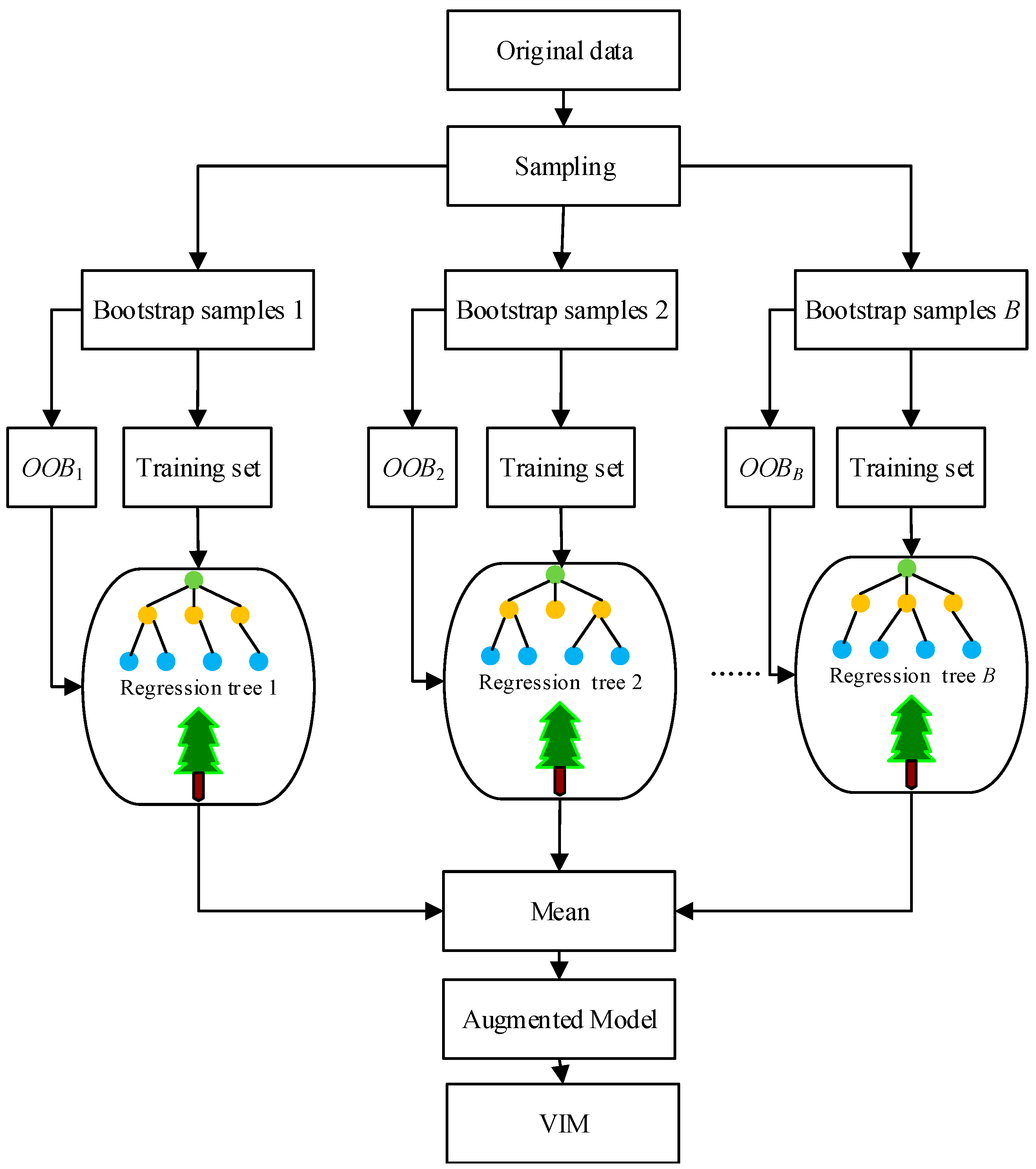
Random forest (RF) is an ensemble machine learning method for improving the performance of classification and regression trees, as well as for reducing overfitting risk. It has become popular since it was brought out and has been widely utilized in many fields such as rainfall forecasting [40], solar radiation forecasting [41], urban water consumption [42], and land cover classification [43]. It is a powerful machine learning tool for identifying features and/or fitting nonlinear relationships for high-dimensional data, especially in the case of small samples. In addition, it also can give an importance score for each input feature variable by permuting each feature.
Since all the data used in this study are time series, the rest of this section is limited to regression issues. For a given input vector X with m features, with a corresponding output vector Y, a training set Sn with n observations can be constructed:
The bootstrap sampling technique is firstly employed to obtain training samples from the original data. A bootstrap sample is generated by randomly selecting n observations with replacements from the original training data. Each observation has the same probability 1/n of being chosen and may appear more than once. The bootstrap samples are used to establish B regression trees, and the rest of the out-of-bag (OOB) data are applied to verify the performance of the built regression trees. All these trees compose a random forest, as shown in Figure 1. The final prediction results of the RF are obtained by aggregating all the regression trees. The prediction precision of each regression tree can be represented by the mean squared error (MSE) between the predicted values and the observed values of the OOB data.
The i-th regression tree Tb (b = 1, 2, …, B) is employed to predict the output of .
There are many factors affecting the generation of streamflow, and these factors interact with each other. The correlations between variables must be considered in the process of determining the RF importance measure. The procedure of RF for estimating the correlated variable importance measure can be briefly described as follows:
Step 1. Estimate the mean vector and covariance matrix from the original data .
Step 2. Grow unpruned regression trees Tb (b = 1, 2, …, B) to fit the bootstrap samples.
Step 3. Use the regression trees Ti to forecast the corresponding OOB data, where the estimation is .
Step 4. Divide the into two parts: vector and matrix .
Step 5. Generate a new matrix and vector on the basis of vector and matrix . Their mean vectors and covariance matrices are different from the original and , and the new ones should be used in the transformation process. For the multivariate normal distribution, , ,, and can be calculated as shown below.
The and of X can be written as:
The conditional mean vector and covariance matrix can be acquired via:
After that, the Nataf transform can be used to generate the normal correlation samples and .
Step 6. Construct new matrices and based on matrix , vector , and matrix .
Step 7. Use the regression tree to predict the response of and the response of , respectively. The errors of the correlated variables can be obtained, and the average values are the impact of variable Xi.
2.3. Gaussian Process Regression
GPR, a very well-known machine learning (ML) method, is a nonparametric Bayesian approach [44]. It was developed by combining Bayesian and statistical theory. This method not only inherits the flexible inductive reasoning ability of Bayesian methods but also has the parallel processing, self-organizing, adaptive, and self-learning abilities of ML. Hence, it has obvious advantages in solving high-dimensional complex nonlinear regression problems with few samples. These characteristics mean that GPR is widely applied in theoretical research and many practical engineering problems [38].
Given a training set with n observations, where y is the variable to be predicted (such as monthly streamflow), X is the input vector for y with m-dimensional factors. In the GRP model, the input vector X and the target output y should obey the following equation:
where represents the latent nonlinear function and its prior probability distribution, is a Gaussian distribution, the random residuals are assumed to have iid Gaussian distributions with mean 0 and variance , and is the n-dimensional unit matrix.
The stochastic process state set of the input variable X follows an n-dimensional joint Gaussian distribution. According to the definition of a Gaussian process, the state set g of the stochastic process is a Gaussian process, and its probability function, denoted GP, can be uniquely determined by its mean function and covariance function matrix .
According to the properties of GP, the target output y of the training input sample Sn and the output of testing sample follow the multivariate Gaussian distribution as follows:
where is the covariance matrix of the testing input set and the training input variables X, and is the covariance for itself.
Under the given conditions of the training input data X and output y, the posterior distribution of the predicted value can be inferred according to the Bayesian posterior probability mathematical formula of the new input :
where is the expected value of and is the posterior variance for , to measure the uncertainty of the predicted results.
Based on the above statement, a GP can be determined by its mean function and the covariance function (CoF) matrix. The standard GP can be transformed into a Gaussian distribution with a mean function of 0. Hence, the key task of solving the GPR model is to determine its covariance function. The GPR requires that its covariance function is a positive definite matrix in the case of a finite input sample size. The above requirements satisfy the Mercer theorem, so the covariance function of the GPR is also called a kernel function and is used to measure the fitting degree between the measured value and the predicted value. There are a variety of choices for the CoF, among which the isotropic squared exponential covariance function (covSEiso) is the most widely used, because the covSEiso has the characteristic of being infinitely differentiable and can then ensure that the GPR is very smooth. Its mathematical expression is:
where is the signal variance linked to the general function variance and l is the scale of the variance. In addition, gives the local correlation and l characterizes the correlation between the input and output. A smaller value of l means that the predicted results of the model change rapidly in the input space, indicating weak correlation.
Generally, is called the hyperparameter set for the CoF of the GPR. The most commonly used method for solving hyperparameters is the maximum likelihood function (MLF). MLF is used to estimate the unknown hyperparameters from the training data by inference. In this process of inference, the conditional probability of the training sample is calculated first, and then its likelihood function can be obtained. The mathematical expression for is:
Next, the derivative of at is calculated as:
Finally, the optimal can be obtained by minimizing the above partial derivative equation using conjugate gradient, Newton’s method, and other optimization algorithms. Once the optimal is obtained, the expected value and the posterior variance of can be calculated using Equation (9).
According to the sigma rule for Gaussian distributions, the confidence interval of the predicted value for a given confidence level 1-α can be obtained as follows:
3. Framework and Procedure of the Proposed Model
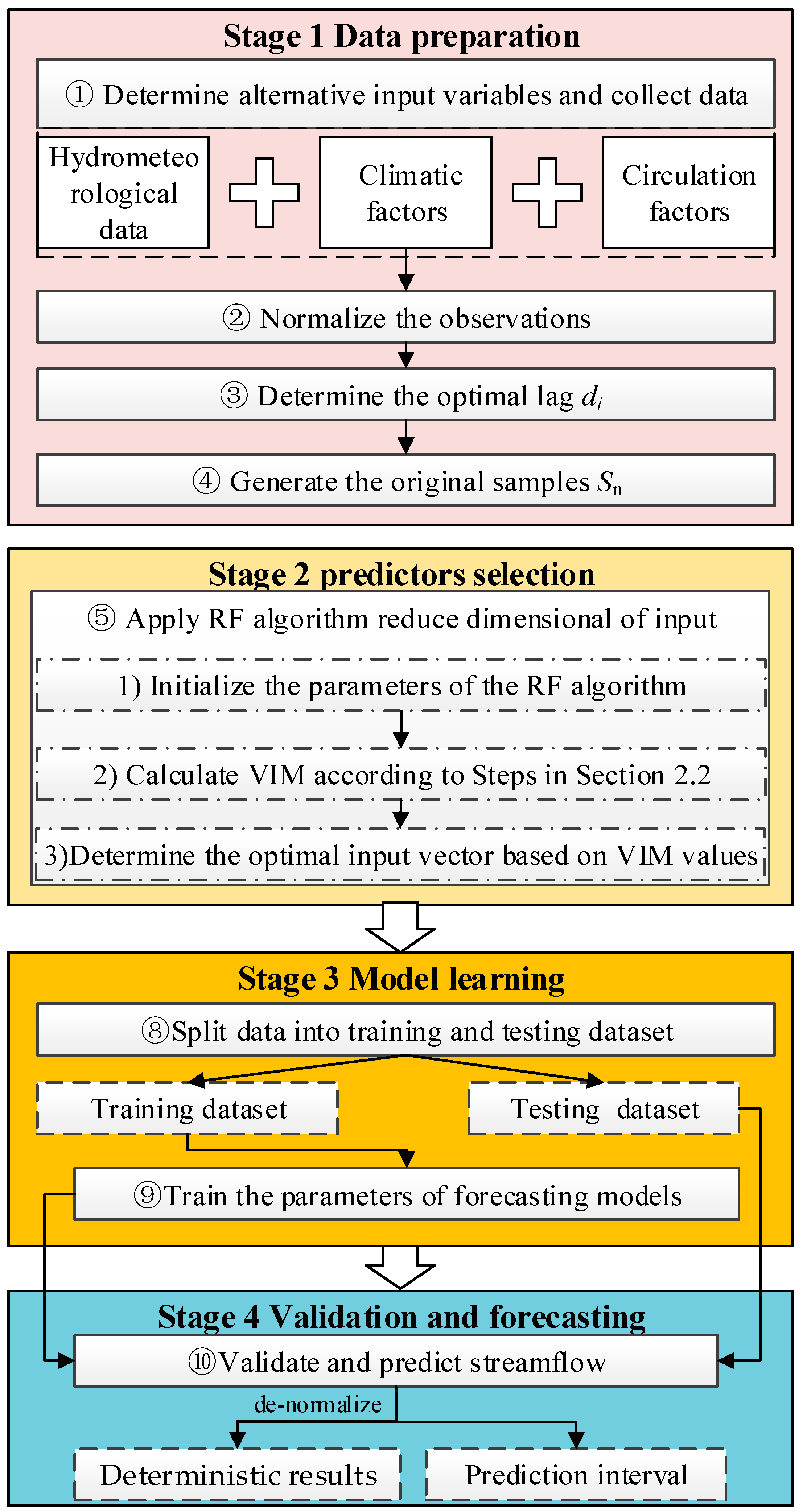
Traditional DDMs for monthly streamflow forecasting lack physical mechanisms and usually provide deterministic results with a single streamflow value. They have limited capacity to forecast streamflow with nonlinear, highly irregular, non-stationary characteristics. Thus, they provide limited and less reliable information for activities related to water resource management. Therefore, in this study, an MVDSF framework is developed. It is realized by integrating RF and GPR with multi-scale variables (hydrometeorology, climate predictors) as inputs and is referred to as RF-GPR-MV. This framework contains four main stages: (1) data preparation, (2) selection of predictors, (3) model learning, and (4) validation and forecasting. In the first stage, contemporaneous data regarding hydrometeorology and climate variables associated with streamflow are collected. In the second stage, RF is applied to filter the dominant variables by discarding redundant and irrelated information, thereby reducing the dimension of the input vector. This can save time and decrease the risk of overfitting. In the third stage, GPR based on Bayesian theory is adopted to simulate the nonlinear relationships between the optimal input vector and the streamflow for a specific location. In the last stage, the optimized GPR is applied to predict the testing dataset. A diagram of the MVDSF framework is shown in Figure 2, and the RF-GPR-MV procedure is summarized as follows:
Step 1: Make a preliminary determination of the alternative input variables and collect their historical observations.
According to the formation mechanism for streamflow, the alternative input factors can be selected and constructed from many related variables such as hydrological and meteorological variables, climate factors, and circulation indices that drive the operation of the water cycle system.
Step 2: Normalize the observations.
The potential input variables have local and teleconnected relationships with runoff, and they have different physical dimensions. Therefore, all these observations must be normalized in this step to eliminate the influence of physical dimensions.
Step 3: Determine the optimal lag di (i = 1, 2,…, m).
The response time of runoff to different variables is different. A PACF (partial autocorrelation function) is used to determine the optimal lag for each variable by forming predictors.
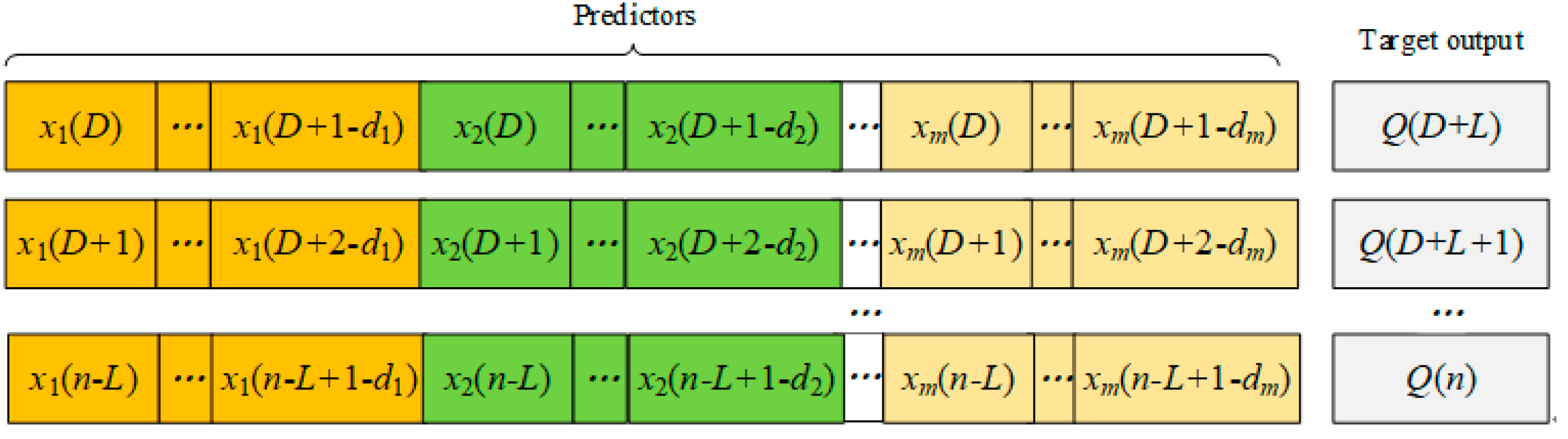
Step 4: Generate the original samples Sn.
The Sn = {(X1, y1),(X2, y2), …, (Xn, yn)}, X ∈ Rm, y ∈ R contains input predictors and the target output for different lead times, as shown in Figure 3.
Step 5: Apply the RF algorithm to reduce the dimensions of the input.
Step 5-1: Initialize the parameters of the RF algorithm.
In this step, two key parameters of the RF will be initialized: the number of regression trees B and the maximum number of variables used to grow a regression tree mtry. Generally, mtry is recommended to be m/3, where m is the dimension of the alternative input vector.
Step 5-2: Calculate the VIM according to the steps in Section 2.2.
Step 5-3: Determine the optimal input vector based on the VIM values.
List the VIM in descending order. Then, the variables with higher VIM values are selected.
Step 6: Split the data obtained in Step 5 into training and testing datasets.
The normalized data obtained in Step 5 are split into two sets: the training and testing datasets. In this study, the training and testing datasets account for 75% and 25%, respectively, of the monthly data.
Step 7: Train the parameters of the GPR forecasting model.
The training dataset is used to construct the GPR and learn its hyperparameters.
Step 8: Validate and predict the streamflow.
The testing dataset is applied to cross-validating and forecasting the streamflow using the optimized model produced by Step 7. The output runoff values of the forecasting model should be denormalized to the range of the target output dataset. Then the RF-GPR-MV model outputs the deterministic results and the corresponding prediction interval.
Note that the differences between the five models (RF-GPR-MV, PCC-GPR-MV, PCC-GPR-QP, PCC-BP-QP, and PCC-GRNN-QP) involved in this study are in Step 1, Step 5 and/or Step 7. For example, in PCC-BP-QP, the previous runoff and precipitation are collected in Step 1, the PCC is applied to select the input variables in Step 5, and the parameters of BP are trained in Step 7.
4. Case Study
4.1. Study Area
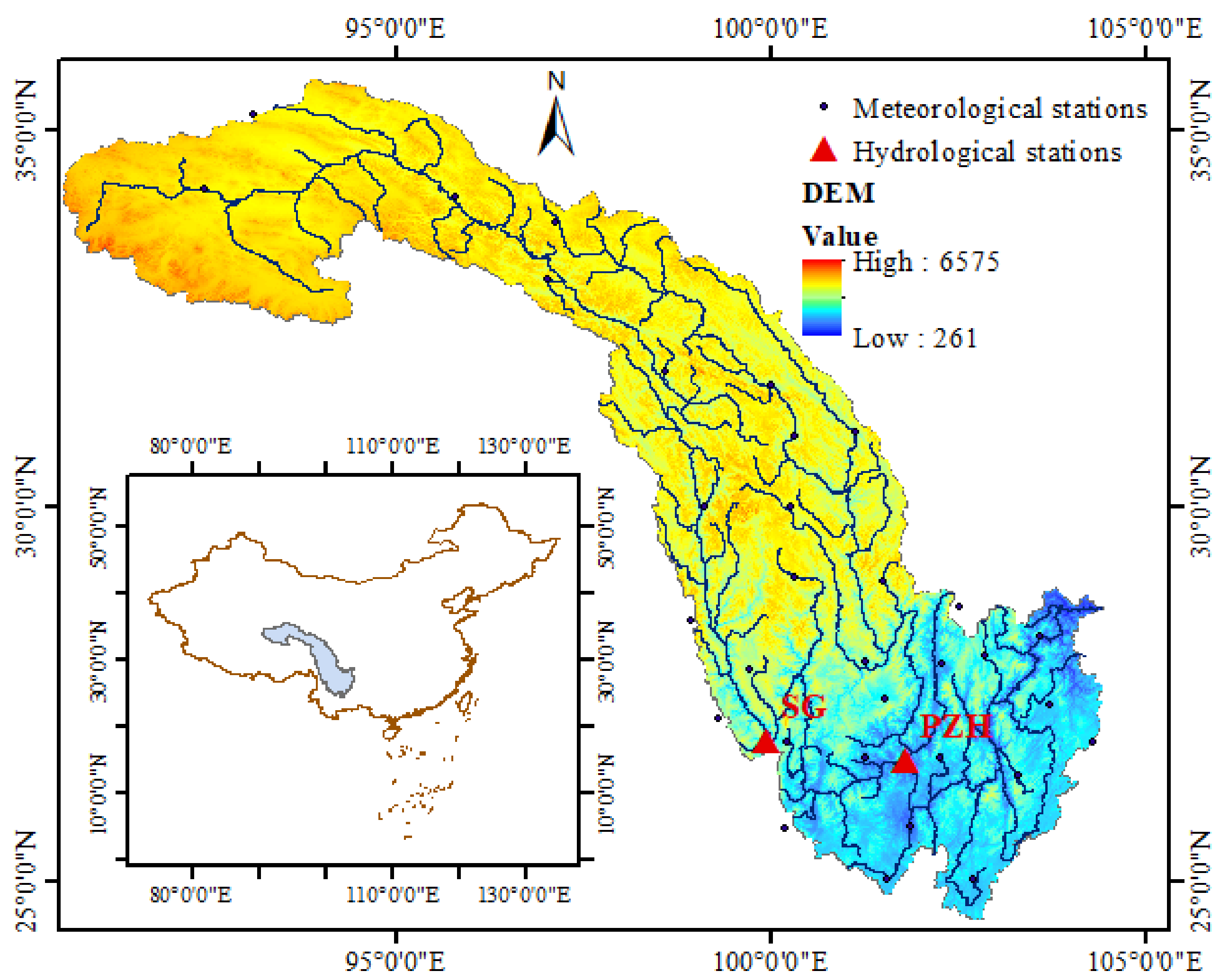
The Jinsha River basin, located in Southwest China (as shown in Figure 4), was chosen to demonstrate the ability of the proposed forecasting model to capture the climate–hydrological relationship of the water cycle system. The Jinsha River basin covers an area of approximately 473,000 km2 and is located approximately between 90°23′ and 104°37′ E and between 24°28′ and 35°46′ N. Most of the landscape in this region is mountainous. The Jinsha River basin basically belongs to the plateau climate zone. From north to south, it can be divided into the sub-arid climate zone of the plateau sub-cold zone, the humid climate zone of the plateau sub-cold zone, and the humid climate zone of the plateau temperate zone. The main stream of the Jinsha River has many merits, including abundant and stable runoff, a large river drop, abundant hydropower resources, and good development conditions. The region is rich in water resources and is one of the world’s water resources enrichment areas. Due to these merits, it has been the largest hydropower energy base in China, and it plays an important role in the Chinese project “West–East Electricity Transmission Project”. The main rainfall season is from May to September, with a flooding season from June to September. Owing to ubiquitous human activities and global warming, it is very difficult to find a basin that is not affected by natural and/or human factors such as abnormal climatic change, irrigation, water resources engineering projects, and land cover/use change [10]. Therefore, in this paper, we propose a novel data-driven model to better characterize the notoriously nonlinear and non-stationary streamflow, in order to better serve the region’s water resources management.
4.2. Data Description and Potential Predictors
Typically, streamflow is affected by many factors, mostly associated with geographic and climatic conditions. Most previous studies focus on local meteorological factors dominated by geographic conditions [9]. Many of these have demonstrated that precipitation has a great influence on both short- and long-term streamflow. Hence, in this paper, the current and antecedent total monthly precipitation was chosen as one of the candidate impact factors (IFs). Previous precipitation can indicate the initial wetness conditions of the study area. Antecedent streamflow is also considered, as it usually represents the comprehensive states of the soil moisture and groundwater stores. Meanwhile, the initial catchment conditions also affect the generation of streamflow. For example, the states of the soil moisture and groundwater storage are relevant to the infiltration process of the hydrologic cycle, thus affecting the streamflow. Therefore, the average temperature, air pressure, and relative humidity were also selected as candidate predictors for streamflow forecasting.
In addition to the above regional meteorological variables representing the initial catchment conditions, some large-scale factors such as global climate variables [23,45] and atmospheric circulation are also considered, to represent the climate variability. Based on a great deal of previous research in the Jinsha River basin and in China on the local influence of large-scale atmospheric circulation, the Pacific decadal oscillation (PDO) [46], the North Atlantic oscillation (NAO) [47], the Atlantic multidecadal oscillation (AMO) [48], the sea surface temperatures (SSTs) over various Niño regions [49], the Pacific/North American pattern (PNA) [50], the Arctic oscillation (AO) [48], the quasi-biennial oscillation (QBO) [51], and the East Atlantic/West Russia (EA/WR) pattern [48] were identified as candidate predictors. Meanwhile, 17 circulation factors from 74 characteristic atmospheric oscillation factors provided by the Chinese National Climate Center (https://cmdp.ncc-cma.net/cn/prediction.htm, accessed on 1 January 2022) were also adopted. A summary of the candidate predictors is given in Table 1.
The datasets used in this study were as follows:
(1) Observed streamflow
The monthly streamflow of two hydrological stations, named Shigu (SG) and Panzhihua (PZH), in the Jinsha River basin, from 1961 to 2010, were collected from the Bureau of Hydrology, Changjiang Water Resources Commission.
(2) Local meteorological variables including precipitation, air pressure, temperature, and relative humidity
These data, at a daily scale for 32 meteorological stations from 1961 to 2010, were downloaded from the Chinese National Meteorological Information Center (http://www.nmic.cn/, accessed on 12 April 2022). The daily meteorological data were then transformed into a monthly scale. Observations collected at one location cannot describe the meteorological conditions of the entire basin. Hence, the weight of each meteorological station was calculated using the Thiessen polygon method (TPM), and then the areal observed values for the corresponding meteorological variables in the studied area were obtained.
(3) Global climate or circulation factors
Variables 5 to 21 in Table 1 at a monthly scale were obtained from the Chinese National Climate Center (NCC). Other global climate factors (22 to 33 in Table 1) were retrieved from the Earth System Research Laboratory of the National Oceanic and Atmospheric Administration (https://www.esrl.noaa.gov/psd/data/climateindices/list/, accessed on 12 April 2022). Observations of SASMI and EASMI from June to August were retrieved from the College of Global Change and Earth System Science at Beijing Normal University (http://ljp.gcess.cn/, accessed on 1 January 2022).
Observations of meteorological, climate, and circulation factors, were collected for the same period of streamflow.
4.3. Model Input Predictor Selection
After determining the potential predictors and collecting their homochronous data, the potential input vectors can be established. The input selection technique was applied to determine suitable input vectors from the large number of candidate IFs, to reduce the amount of redundant and irrelevant information. Finally, the most relevant input vectors with the lowest dimensions were found.
We take the SG station as an example to show the rule for the establishment of potential input vectors. The monthly streamflow of the SG station in January of the following year was taken as the prediction variable. Alternative input vectors were established that included three parts:
- (1)
- Observations of streamflow with a lag of 1 to 12 months;
- (2)
- Local meteorological variables, global circulation factors, and climate factors (listed in Table 1 Nos. 1–33) with lags of up to 12 months;
- (3)
- Observations of the SASMI and EASMI from June to August in the last year.
In summary, there were 34 × 12 + 3 × 2 = 414 potential input factors, as shown in Table 2. The same potential input vector was used for the other 11 months in the following year. Then, the potential input vectors for each month in the following year for the other two hydrological stations were constructed in a similar manner.
The fewer the variables in the input vector, the simpler the constructed forecasting model is for training. Therefore, the major concern is to reduce the input dimensions, thereby simplifying the forecasting model. In this study, the RF algorithm was adopted to find the input vector with the lowest dimension. The parameters of the RF were set as B = 500 and mtry = 138, according to [29].
The candidate input vectors for the various models are shown in Table 2.
4.4. Performance Evaluation
There are many measures for evaluating model performance in the published literature. The Nash–Sutcliffe coefficient of efficiency (NSE) is the most widely used. A disadvantage of the NSE is the use of squared differences, which causes larger values in a time series to be strongly overestimated and lower values to be neglected.
The present study also adopted other widely used indices: the Pearson’s correlation coefficient (R), root mean square error (RMSE), mean absolute error (MAE), mean average percentage error (MAPE), mean bias error (MBE), and modified index of agreement (MIA). Among these, the RMSE is sensitive to extremely large or small values of a time series and reflects the degree of variation [52], the MAE reflects the actual forecasting error from a more balanced perspective, the MAPE is a measure of the accuracy for the forecasted streamflow series with no units, the MBE is a measure of the overall bias error or systematic error, and the MIA is a standardized measure of the degree of model prediction error [53]. Usually, the RMSE is higher than the MAE, and the degree to which the RMSE exceeds the MAE is an indicator of the extent to which large outliers (differences between observed values and the corresponding forecasts) exist in the testing set [34].
These indices are defined as follows:
where and are the i-th observed and predicted values of streamflow, respectively, and are the average values of the observed and forecasted streamflow, respectively, and N is the total number of samples.
5. Results and Discussion
5.1. Results with Only Previous Q and P as Inputs
Forecasting results with different lead times using previous streamflow and precipitation for the two stations are shown in Figure 5 and Figure 6, where the red dashed line is the threshold of 0.7 for the NSE. For example, with regard to the forecast model for SG station, the validation period NSE values for 1- to 3-month-ahead forecasting were equal to 0.87, 0.75, and 0.71 for the PCC-GPR-QP model, compared to values of 0.81, 0.56, and 0.55 for the PCC-BP-QP model and 0.76, 0.32, and 0.38 for the PCC-GRNN-QP model. Further analysis shows that the MAPE values for the 1- to 3-month-ahead forecasting associated with PCC-GPR-QP were 5%, 6%, and 5%; less than the values for the PCC-BP-QP and PCC-GRNN-QP models.
Similarly, for PZH station, PCC-GPR-QP gave NSE values for 1- to 3-month-ahead forecasting of 0.96, 0.93, and 0.52, compared to values of 0.88, 0.31, and 0 for PCC-BP-QP and 0.84, 0.65, and 0.25 for PCC-GRNN-QP. In addition, the MAPE values for 1- to 3-month-ahead forecasting associated with the PCC-GPR-QP model were 2%, 2%, and 4%; less than for the other models under investigation.
The NSE values presented in these figures provide a clear picture of the poor accuracy of the forecasting results. Specifically, for PCC-GPR-QP, the lead time 1 and lead time 2 forecasting results for these two stations have relatively high accuracy, as their NSE values exceed the threshold of 0.7. For PCC-BP-QP, the lead time 1 forecasting results for the two stations have acceptable accuracies, with NSE values beyond the threshold of 0.7. For PCC-GRNN-QP, the lead time 1 forecasting results for stations SG and PZH have relatively good accuracies, with NSE values beyond the threshold of 0.7. Therefore, the sequence of forecasting ability for a short lead time is: GPR > BP > GRNN. Clearly, the degree of deterioration becomes dramatic as the forecast period increases, especially for GRNN and BP with long lead times.
Overall, for the same inputs and lead times, the GPR always outperforms the BP and GRNN models and has a stronger anti-disturbance ability than the other two models, and therefore it is suitable as a basic forecasting module. However, the forecasting results for PCC-GPR-QP with a lead time beyond 4 still have room for improvement.
5.2. Results with Local Hydrometeorological and Global Factors as Inputs
The validation results for the proposed model, RF-GPR-MV, and PCC-GPR-MV are listed in Table 3, Table 4, Table 5 and Table 6, where the NSE values beyond the threshold of 0.7 are marked in bold. Meanwhile, Figure 7 and Figure 8 show the forecasting results with different lead times visually, using both hydrometeorological and global climate factors as inputs for the two stations. The results show that multi-variable nonlinear RF-GPR-MV models are, in general, superior to the PCC-GPR-MV model, the PCC-GPR-QP model, the PCC-BP-QP model, and the PCC-GRNN-QP model.
Regarding SG station, the validation period NSE values for lead times 1, 2, 3, and 10 forecasting results for the RF-GPR-MV model were 0.88, 0.78, 0.72, and 0.78, respectively, which are over the threshold of 0.7, indicating good accuracies. Those of the other lead time forecasting results, except for lead time 8 (0.29), were all beyond the threshold of 0.5, representing acceptable accuracies. The validation period NSE values for lead times 1, 2, and 3 forecasting results for PCC-GPR-MV were 0.87, 0.75, and 0.71, respectively, surpassing the threshold of 0.7, but those for the other lead times were all under the threshold of 0.5. Clearly, for the same lead time, the NSE values for RF-GPR-MV were higher than those for PCC-GPR-MV. Additionally, for the same lead time, the validation period R and the MAPE values for RF-GPR-MV have considerable accuracies or superior accuracies to those of PCC-GPR-MV.
With regard to PZH station, the validation period NSE values for the lead time 1, 2, 3, 7, 11, and 12 forecasting results for RF-GPR-MV were 0.96, 0.94, 0.76, 0.74, and 0.71, respectively, exceeding the threshold of 0.7, indicating high accuracies. Those for the other lead time forecasting results were all beyond or close to the threshold of 0.5, representing acceptable accuracies. The validation period NSE values for the lead time 1 and 2 forecasting results for PCC-GPR-MV were 0.95 and 0.94, surpassing the threshold of 0.7, but those for the others were all under the threshold of 0.5, except for that of lead time 3 (0.52), which was close to the threshold of 0.5. Additionally, in the analysis of the validation period R and MAPE values, those associated with RF-GPR-MV were considerable or superior to those of PCC-GPR-MV.
Compared with the performance of PCC-GPR-QP, that of PCC-GPR-MV showed no obvious improvement, while RF-GPR-MV showed significant enhancement. This indicates that the PCC may not be suitable for complex nonlinear relationship extraction, especially for teleconnection. Specifically, the comparison of PCC-GPR-MV and RF-GPR-MV indicates that RF-GPR-MV has lower MAPE, RMSE, and MBE, as well as higher R, NSE, and MIA values than PCC-GPR-MV for almost all lead times. In summary, RF-GPR-MV integrates the dimensionality reduction advantage of RF and the strong learning and reasoning ability of GPR to fully extract the effective information for learning and then further improve the prediction accuracy.
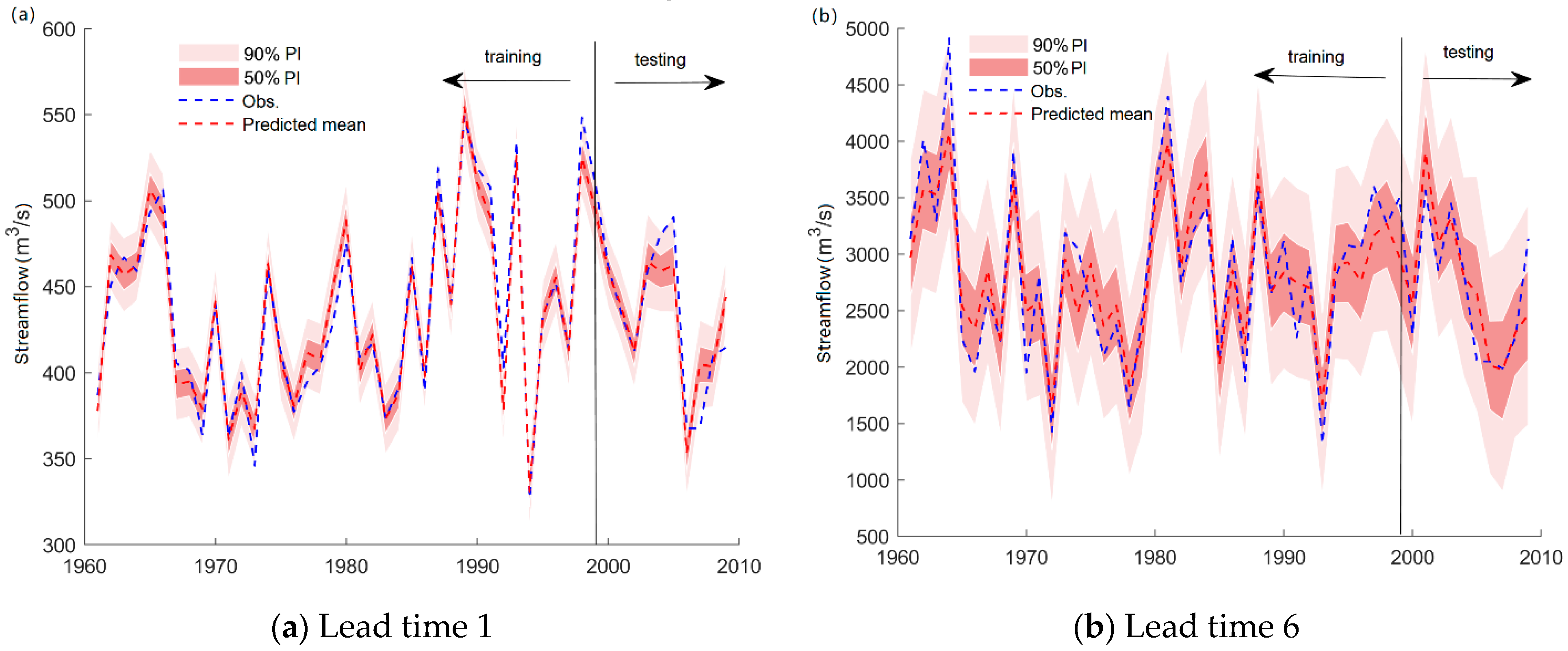
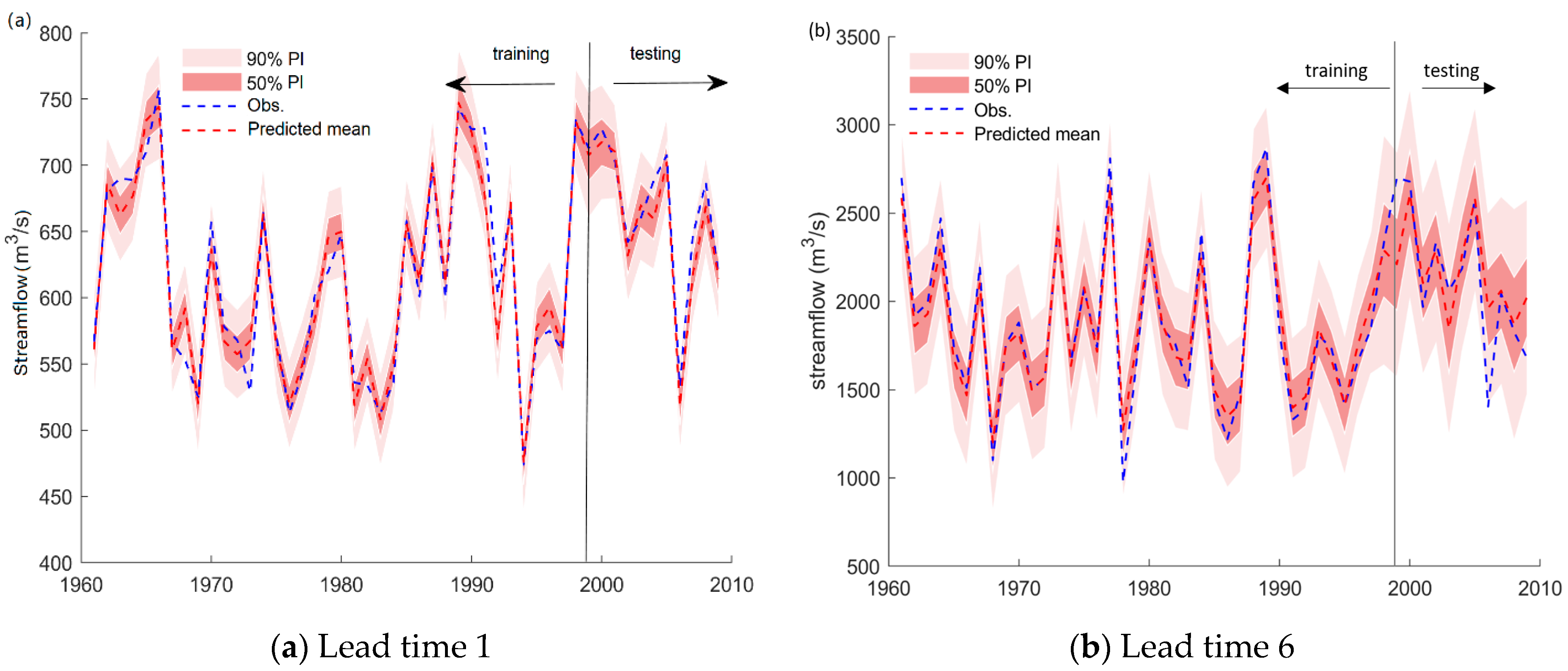
Figure 9 and Figure 10 present the hydrograph produced by the RF-GPR-MV model in the training and testing periods. The reason for choosing the results for lead times 1 and 6 is that the observed streamflow was relatively stable when the lead time was 1, and the observed runoff fluctuated greatly when the lead time was 6, as this was close to the flood season. It shows that the prediction intervals (PIs) at the 50% confidence level generated by RF-GPR-MV can always capture the variations in streamflow during the testing phase. For both stations, the prediction interval for 6-month-ahead forecasting was significantly wider than that for 1-month-ahead forecasting, indicating a relatively high uncertainty. Although the uncertainties of forecasting with long lead times are large, they still fall within the given prediction intervals (PIs) at the 50% confidence level, except in some extremely high flow conditions.
Overall, the proposed RF-GPR-MV model using both local hydrometeorological and global climate and circulation factors not only has higher accuracy than the commonly used monthly streamflow forecasting models but can also provide both deterministic results and uncertainty bounds.
5.3. Evaluation of the Contributions of Different Factors
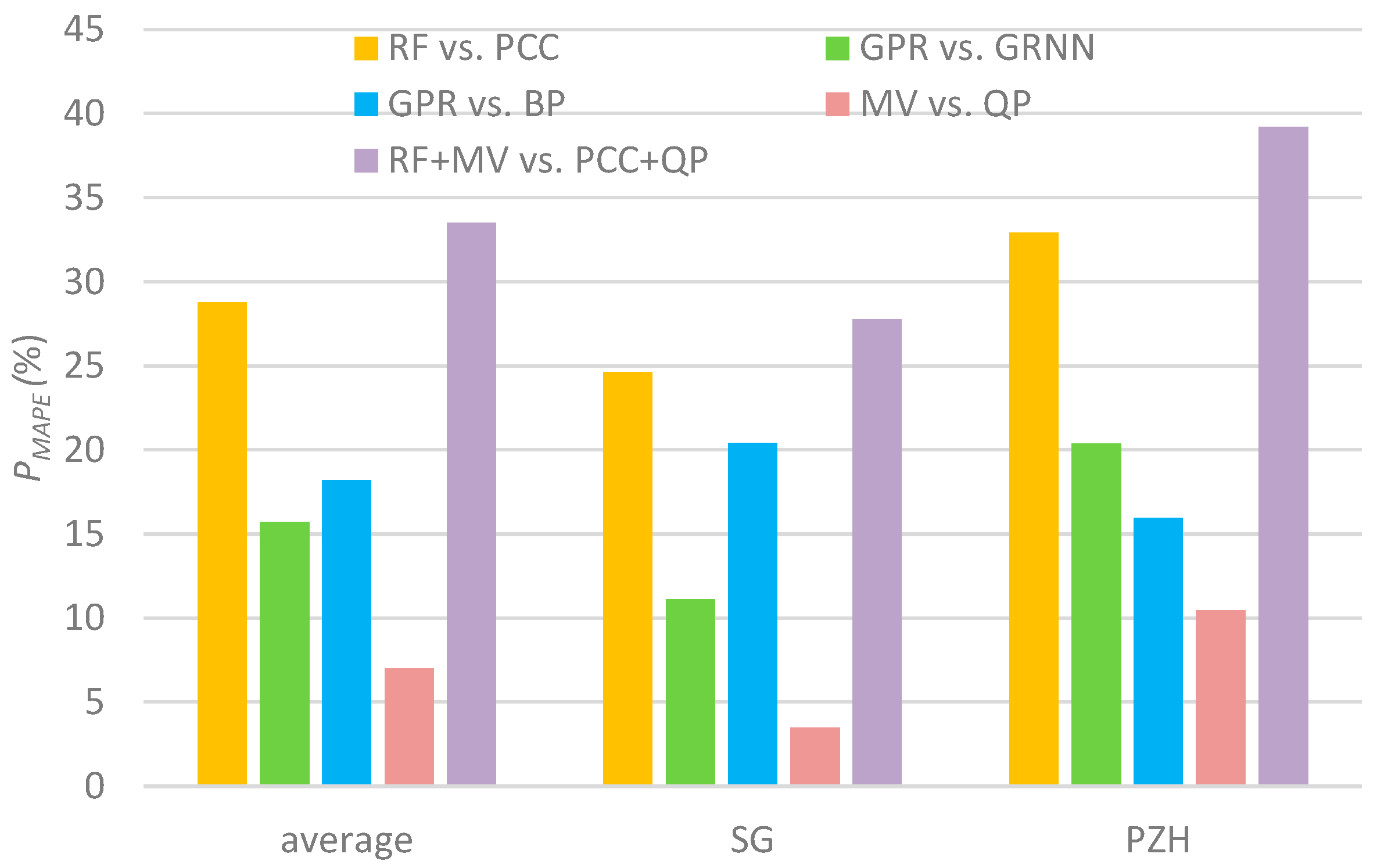
To quantitatively evaluate the improvement achieved by the proposed RF-GPR-MV model over the RF-GPR-QP, PCC-GPR-MV, PCC-GPR-QP, PCC-BP-QP, and PCC-GRNN-QP models, the improved percentages of the MAPE index were adopted to evaluate the impacts of the different techniques on the improvement of the hybrid model. PMAPE is defined by: , where MAPE1 and MAPE2 are the MAPE values of model 1 and model 2. Figure 11 quantitatively displays the contributions made by the RF method, the GPR model, and/or the multiple variables (MV) as inputs to the total improvement of the RF-GPR-MV model. Clearly, all these had positive effects on the total improvement of the proposed model, though RF (average PMAPE = 27%) contributed more than GPR (average PMAPE = 16%), which emphasizes the critical role of the input selection approach in monthly streamflow forecasting. Additionally, compared with using only previous streamflow and rainfall, using multiple variables (MV) as inputs improved the model performance by about 5%.
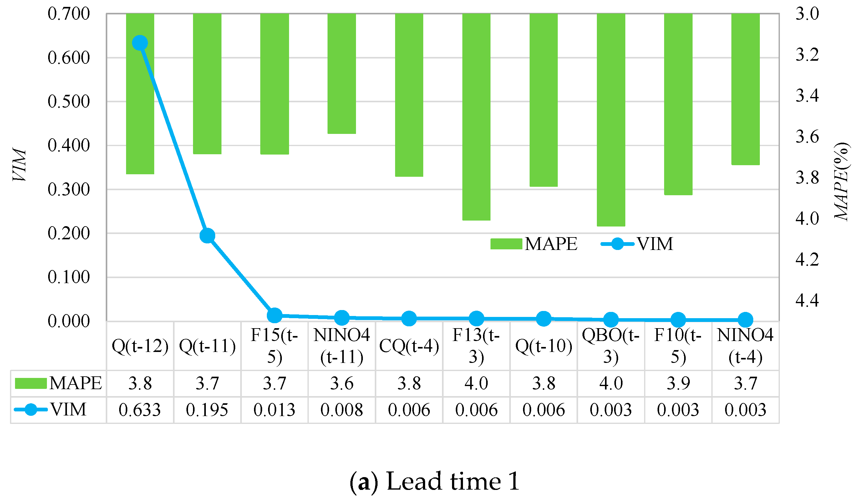
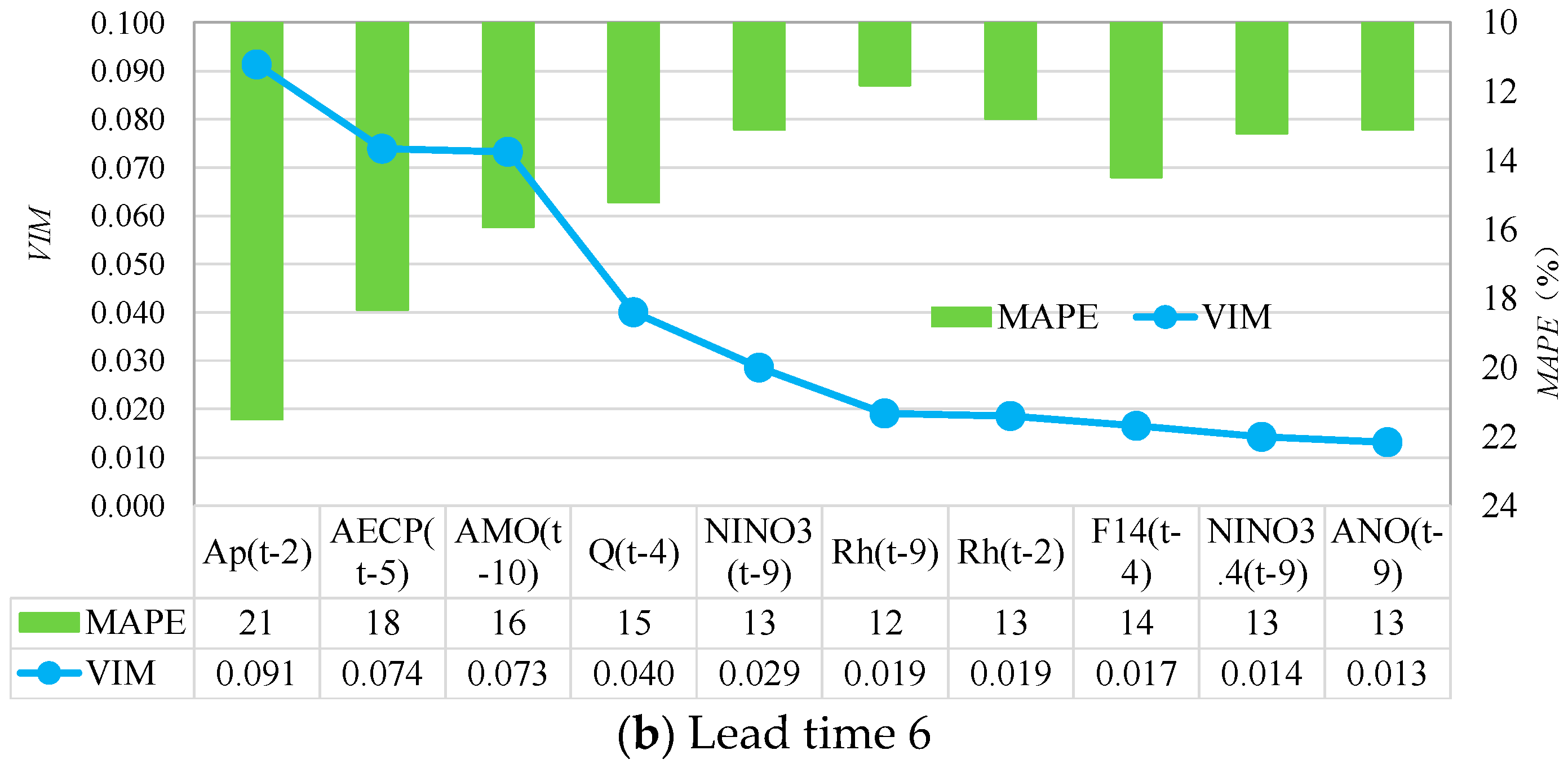
Further, to quantify the contribution of large-scale factors to the model performance for different lead times, RF-GPR-MV was used, and the VIM values in descending order with the top 10 input factors provided by RF and the MAPE values for their corresponding forecasting models were compared with each other. For example, Figure 12 and Figure 13 present the monthly streamflow forecasting results for RF-GPR-MV with lead time 1 (January of the following year) and lead time 6 (June of the following year) using different inputs at SG station and PZH station, respectively.
It can be seen from Figure 12a that the forecasting results for RF-GPR-MV with lead time 1 achieved the smallest forecasting error when taking Q(t-12), Q(t-11), F15(t-5), and Niño4(t-11) as inputs. In this case, the contribution of Q(t-11) was 2.6%; when adding F15(t-5) and Niño4(t-11) as inputs, the forecasting performance was improved by 2.69% over Q(t-12) only. This shows that the contribution of the streamflow itself was greater than the contribution of large-scale climate factors for forecasting with short lead times (dry season). The results for RF-GPR-MV with lead time 6 (Figure 12b) obtained the best performance when using all the top ten factors, including the local hydrometeorological indices P(t-2), Q(t-4), and P(t-8), the global climate factors AO(t-9), NAO(t-11), PDO(t-1), and NAO(t-2), and the circulation factors F10(t-2), F11(t-2), and SOI(t-10). Among these, the highest contribution to the monthly streamflow forecasting came from F10(t-2) (16%), followed by PDO(t-1) (15%), indicating the importance of large-scale factors in the flood season.
Figure 13a shows that the forecasting results for RF-GPR-MV with lead time 1 at PZH station achieved the lowest MAPE value when using the local hydrometeorological factors Q(t-12), Q(t-11), Q(t-9), Ap(t-9), and Q(t-10). Figure 12b shows that the forecasting results with lead time 6 showed the best performance when taking Ap(t-12), AECP(t-5), AMO(t-10), Q(t-4), Niño3(t-9), and Rh(t-9) as inputs. In this case, the best input vector contained many types of variables varying from local hydrometeorological factors (Ap, Q, Rh) to large-scale climate factors (AECP, AMO, Niño3). Additionally, the forecasting performance using Q(t-4) was better by about 5% than when not using Q(t-4), while the forecasting performance with Niño3(t-9) was better by about 14% than without Niño3(t-9). This result confirms that large-scale climate factors have a great influence on local streamflow with long lead times (flood season).
These figures (Figure 11, Figure 12 and Figure 13) emphasize that the addition of global climate and circulation factors can improve the forecasting performance for streamflow, especially for forecasting with long lead times. They also indicate that when the number of prediction factors continues to increase, the model’s prediction error will also increase. This phenomenon reveals that increasing the number of input factors is not always beneficial to the forecasting results. The best results are obtained with just the appropriate number of input factors.
5.4. Discussion
In this study, for SG station, the model efficiencies (in terms of the NSE) for 1-month-ahead forecasting for the PCC-GRNN-QP, PCC-BP-QP, PCC-GPR-QP, PCC-GPR-MV, and RF-GPR-MV models were found to be 0.76, 0.81, 0.87, 0.87, and 0.88, respectively. For PZH station, the NSE and MAPE values for RF-GPR-MV for 1-month-ahead forecasting were 0.96 and 2%, respectively.
In a previous study, Peng et al. [54] employed pure BP, PSO-ANN, and MVO-ANN models for the Jinsha basin at PZH station and achieved a model efficiency (in terms of MAPE) of 10%, which is much higher than that of the RF-GPR-MV model developed in this study. In the study by Yin et al. [55], a SWAT model using meteorological data and the ISI-MIP climate dataset was employed for the Jinsha basin for monthly streamflow forecasting, achieving a model efficiency (in terms of the NSE) of 0.82, which is lower than that of the RF-GPR-MV developed in this study. Moreover, in the study by Luo et al. [56], autocorrelation function (ACF), partial autocorrelation function (PACF), grey correlation analysis (GCA), support vector regression (SVR), and generalized regression neural network (GRNN) models were integrated to forecast monthly streamflow in the Jinsha basin. In this study, the NSE values for GCA-SVR, GCA-GRNN, PCC/ACF-SVR, and PACF-SVR were 0.86, 0.82, 0.83, and 0.82, respectively. The NSE value for the best model (GCA-SVR) was 0.86, which is still lower than that of the RF-GPR-MV model developed in this study.
In most of the studies employing ML models [2,13,28,54], only previous streamflow and/or precipitation were taken as inputs. The results in this study revealed the positive effect of climate factors on streamflow forecasting accuracy. This conclusion is consistent with those of other studies [22,23,24,45,56]. In previous studies based on ML models, inputs were determined by a trial-and-error method or the PACF method. Input selection is a vital task in the process of data-driven model development. The PACF method is a method of mining linear relationships. However, the correlations between streamflow and its potential forecasting factors are not always linear. The RF in this study used to determine the appropriate input combination reduced the workload and could deal with nonlinear relationships. Additionally, the RF-GPR-MV model developed in this study could provide both deterministic results and prediction intervals, which is beneficial for real water resources management.
6. Conclusions
In recent years, due to the impact of climate change, the non-stationary and nonlinear properties of monthly streamflow have been enhanced, which makes it difficult to improve forecasting accuracy. To improve the accuracy of monthly streamflow forecasting and provide better information for water resources management, a novel MVDSF framework was proposed and realized using RF-GPR-MV. It was used to develop a 1- to 12-month-ahead streamflow forecast model for two sites within the Jinsha River basin. Besides the commonly used local hydrometeorological factors (e.g., previous streamflow and antecedent precipitation), multiple large-scale climate and circulation factors were considered, in order to represent climate change. Therefore, about 400 candidate input factors were constructed. An RF was applied to determine the optimal input from the high-dimensional candidate inputs. Additionally, a GPR was employed to learn the nonlinear relationships between streamflow and its multi-scale predictors and to describe the forecast uncertainty.
The conclusions of the present study are as follows:
- (1)
- The PCC-GPR-QP model yielded better performance compared with the PCC-BP-QP and PCC-GRNN-QP models, which reveals the capability of GPR for dealing with highly nonlinear streamflow. The average forecasting accuracy was improved by 10~20% when using GPR as a forecast module.
- (2)
- The addition of large-scale climate factors significantly improved the long-lead-time forecasting, that is, in the flood season, with an average contribution rate of about 15%.
- (3)
- The RF applied to input selection was beneficial for improving the accuracy of forecasting. Compared with the model using the PCC method, the average forecasting accuracy was improved by 25~30%.
- (4)
- The proposed RF-GPR-MV model was proven to have better modeling accuracy (RMSE, MAE, MBE, and MAPE) and goodness of fit (R, NSE, and MIA) than the other benchmark models (PCC-GPR-MV, PCC-GPR-QP, PCC-BP-QP, and PCC-GRNN-QP). Additionally, the RF-GPR-MV model could provide the prediction interval as supplementary information for practical decision-making.
The accurate and abundant forecast information provided by RF-GPR-MV could help water resources management departments to make scientific decisions to avoid risks. Therefore, this model could be valuable for popularizing this application. Meanwhile, it should be noted that the results of RF-GPR-MV are not ideal under some extremely high flow conditions, and this requires further attention in future studies. Furthermore, the main purpose of this paper was to show that by adding more climate factors and using a reasonable input selection method and a suitable ML model with appropriate parameters, the performance of the monthly streamflow forecasting model could be improved. In future research, other data processing techniques (wavelet transforms, empirical mode decomposition, variational mode decomposition, and so on) and evolutionary algorithms used for optimization of the hyperparameters of the GPR could be considered.
Author Contributions
Conceptualization, N.S., S.Z. and J.Z.; methodology, N.S.; validation, T.P. and S.Z.; writing—original draft preparation, N.S.; writing—review and editing, S.Z., N.Z., H.Z. and T.P.; funding acquisition, J.Z., N.S., N.Z., H.Z. and T.P. All authors have read and agreed to the published version of the manuscript.
Funding
This research was funded by Natural Science Foundation of the Jiangsu Higher Education Institution of China (Nos. 20KJD480003, 19KJB480007, and 19KJB470012), the Natural Science Foundation of Jiangsu Province (No. BK20201069), the National Natural Science Foundation of China (Nos. 91547208 and 51909010), and the Jiangsu Innovative and Entrepreneurial Talents Project (JSSCBS(2020)31035).
Institutional Review Board Statement
Not applicable.
Informed Consent Statement
Not applicable.
Data Availability Statement
The data supporting the findings of this paper are available from the corresponding author upon reasonable request.
Acknowledgments
Not applicable.
Conflicts of Interest
The authors declare no conflict of interest.
References
- Niu, W.-J.; Feng, Z.-K.; Liu, S.; Chen, Y.-B.; Xu, Y.-S.; Zhang, J. Multiple Hydropower Reservoirs Operation by Hyperbolic Grey Wolf Optimizer Based on Elitism Selection and Adaptive Mutation. Water Resour. Manag. 2021, 35, 573–591. [Google Scholar] [CrossRef]
- Lv, N.; Liang, X.; Chen, C.; Zhou, Y.; Li, J.; Wei, H.; Wang, H. A long Short-Term memory cyclic model with mutual information for hydrology forecasting: A Case study in the xixian basin. Adv. Water Resour. 2020, 141, 103622. [Google Scholar] [CrossRef]
- Niu, W.-J.; Feng, Z.-K.; Li, Y.-R.; Liu, S. Cooperation Search Algorithm for Power Generation Production Operation Optimization of Cascade Hydropower Reservoirs. Water Resour. Manag. 2021, 35, 2465–2485. [Google Scholar] [CrossRef]
- Chen, L.; Sun, N.; Zhou, C.; Zhou, J.; Zhou, Y.; Zhang, J.; Zhou, Q. Flood Forecasting Based on an Improved Extreme Learning Machine Model Combined with the Backtracking Search Optimization Algorithm. Water 2018, 10, 1362. [Google Scholar] [CrossRef] [Green Version]
- He, X.; Luo, J.; Zuo, G.; Xie, J. Daily Runoff Forecasting Using a Hybrid Model Based on Variational Mode Decomposition and Deep Neural Networks. Water Resour. Manag. 2019, 33, 1571–1590. [Google Scholar] [CrossRef]
- Tan, Q.-F.; Lei, X.-H.; Wang, X.; Wang, H.; Wen, X.; Ji, Y.; Kang, A.-Q. An adaptive middle and long-term runoff forecast model using EEMD-ANN hybrid approach. J. Hydrol. 2018, 567, 767–780. [Google Scholar] [CrossRef]
- Zhao, X.; Chen, X.; Xu, Y.; Xi, D.; Zhang, Y.; Zheng, X. An EMD-Based Chaotic Least Squares Support Vector Machine Hybrid Model for Annual Runoff Forecasting. Water 2017, 9, 153. [Google Scholar] [CrossRef]
- Shamshirband, S.; Hashemi, S.; Salimi, H.; Samadianfard, S.; Asadi, E.; Shadkani, S.; Kargar, K.; Mosavi, A.; Nabipour, N.; Chau, K.-W. Predicting Standardized Streamflow index for hydrological drought using machine learning models. Eng. Appl. Comput. Fluid Mech. 2020, 14, 339–350. [Google Scholar] [CrossRef]
- Yaseen, Z.M.; Ebtehaj, I.; Bonakdari, H.; Deo, R.C.; Danandeh Mehr, A.; Mohtar, W.H.M.W.; Diop, L.; El-shafie, A.; Singh, V.P. Novel approach for streamflow forecasting using a hybrid ANFIS-FFA model. J. Hydrol. 2017, 554, 263–276. [Google Scholar] [CrossRef]
- Zhou, Y.; Guo, S.; Chang, F.-J. Explore an evolutionary recurrent ANFIS for modelling multi-step-ahead flood forecasts. J. Hydrol. 2019, 570, 343–355. [Google Scholar] [CrossRef]
- Cheng, X.; Feng, Z.K.; Niu, W.J. Forecasting Monthly Runoff Time Series by Single-Layer Feedforward Artificial Neural Network and Grey Wolf Optimizer. IEEE Access 2020, 8, 157346–157355. [Google Scholar] [CrossRef]
- Sun, N.; Zhang, S.; Peng, T.; Zhou, J.; Sun, X. A Composite Uncertainty Forecasting Model for Unstable Time Series: Application of Wind Speed and Streamflow Forecasting. IEEE Access 2020, 8, 209251–209266. [Google Scholar] [CrossRef]
- Granata, F.; Saroli, M.; de Marinis, G.; Gargano, R. Machine Learning Models for Spring Discharge Forecasting. Geofluids 2018, 2018, 8328167. [Google Scholar] [CrossRef] [Green Version]
- Hussain, D.; Khan, A.A. Machine learning techniques for monthly river flow forecasting of Hunza River, Pakistan. Earth Sci. Inform. 2020, 13, 939–949. [Google Scholar] [CrossRef]
- Shu, X.; Ding, W.; Peng, Y.; Wang, Z.; Wu, J.; Li, M. Monthly Streamflow Forecasting Using Convolutional Neural Network. Water Resour. Manag. 2021, 35, 5089–5104. [Google Scholar] [CrossRef]
- Zhu, S.; Luo, X.; Yuan, X.; Xu, Z. An improved long short-term memory network for streamflow forecasting in the upper Yangtze River. Stoch. Environ. Res. Risk Assess. 2020, 34, 1313–1329. [Google Scholar] [CrossRef]
- Kilinc, H.C. Daily Streamflow Forecasting Based on the Hybrid Particle Swarm Optimization and Long Short-Term Memory Model in the Orontes Basin. Water 2022, 14, 490. [Google Scholar] [CrossRef]
- Muhammad, A.U.; Li, X.; Feng, J. Using LSTM GRU and Hybrid Models for Streamflow Forecasting, Machine Learning and Intelligent Communications; Zhai, X.B., Chen, B., Zhu, K., Eds.; Springer International Publishing: Cham, Switzerland, 2019; pp. 510–524. [Google Scholar]
- Wegayehu, E.B.; Muluneh, F.B. Short-Term Daily Univariate Streamflow Forecasting Using Deep Learning Models. Adv. Meteorol. 2022, 2022, 1860460. [Google Scholar] [CrossRef]
- Mosavi, A.; Ozturk, P.; Chau, K.-W. Flood Prediction Using Machine Learning Models: Literature Review. Water 2018, 10, 1536. [Google Scholar] [CrossRef] [Green Version]
- Karamouz, M.; Zahraie, B. Seasonal Streamflow Forecasting Using Snow Budget and El Niño-Southern Oscillation Climate Signals: Application to the Salt River Basin in Arizona. J. Hydrol. Eng. 2004, 9, 523–533. [Google Scholar] [CrossRef]
- Hidalgo-Muñoz, J.M.; Gámiz-Fortis, S.R.; Castro-Díez, Y.; Argüeso, D.; Esteban-Parra, M.J. Long-range seasonal streamflow forecasting over the Iberian Peninsula using large-scale atmospheric and oceanic information. Water Resour. Res. 2015, 51, 3543–3567. [Google Scholar] [CrossRef] [Green Version]
- Risko, S.L.; Martinez, C.J. Forecasts of seasonal streamflow in West-Central Florida using multiple climate predictors. J. Hydrol. 2014, 519, 1130–1140. [Google Scholar] [CrossRef]
- Rasouli, K.; Hsieh, W.W.; Cannon, A.J. Daily streamflow forecasting by machine learning methods with weather and climate inputs. J. Hydrol. 2012, 414–415, 284–293. [Google Scholar] [CrossRef]
- Galelli, S.; Castelletti, A. Tree-based iterative input variable selection for hydrological modeling. Water Resour. Res. 2013, 49, 4295–4310. [Google Scholar] [CrossRef]
- Ren, K.; Fang, W.; Qu, J.; Zhang, X.; Shi, X. Comparison of eight filter-based feature selection methods for monthly streamflow forecasting—Three case studies on CAMELS data sets. J. Hydrol. 2020, 586, 124897. [Google Scholar] [CrossRef]
- Sun, N.; Zhou, J.; Chen, L.; Jia, B.; Tayyab, M.; Peng, T. An adaptive dynamic short-term wind speed forecasting model using secondary decomposition and an improved regularized extreme learning machine. Energy 2018, 165, 939–957. [Google Scholar] [CrossRef]
- Luo, X.; Yuan, X.; Zhu, S.; Xu, Z.; Meng, L.; Peng, J. A hybrid support vector regression framework for streamflow forecast. J. Hydrol. 2019, 568, 184–193. [Google Scholar] [CrossRef]
- Lahouar, A.; Ben Hadj Slama, J. Hour-ahead wind power forecast based on random forests. Renew. Energy 2017, 109, 529–541. [Google Scholar] [CrossRef]
- Pham, L.T.; Luo, L.; Finley, A. Evaluation of random forests for short-term daily streamflow forecasting in rainfall- and snowmelt-driven watersheds. Hydrol. Earth Syst. Sci. 2021, 25, 2997–3015. [Google Scholar] [CrossRef]
- Shen, Y.; Ruijsch, J.; Lu, M.; Sutanudjaja, E.H.; Karssenberg, D. Random forests-based error-correction of streamflow from a large-scale hydrological model: Using model state variables to estimate error terms. Comput. Geosci. 2022, 159, 105019. [Google Scholar] [CrossRef]
- Adnan, R.M.; Zounemat-Kermani, M.; Kuriqi, A.; Kisi, O. Machine Learning Method in Prediction Streamflow Considering Periodicity Component. In Intelligent Data Analytics for Decision-Support Systems in Hazard Mitigation: Theory and Practice of Hazard Mitigation; Deo, R.C., Samui, P., Kisi, O., Yaseen, Z.M., Eds.; Springer Singapore: Singapore, 2021; pp. 383–403. [Google Scholar]
- Yaseen, Z.M.; Mohtar, W.H.M.W.; Ameen, A.M.S.; Ebtehaj, I.; Razali, S.F.M.; Bonakdari, H.; Salih, S.Q.; Al-Ansari, N.; Shahid, S. Implementation of Univariate Paradigm for Streamflow Simulation Using Hybrid Data-Driven Model: Case Study in Tropical Region. IEEE Access 2019, 7, 74471–74481. [Google Scholar] [CrossRef]
- Maheswaran, R.; Khosa, R. Wavelet–Volterra coupled model for monthly stream flow forecasting. J. Hydrol. 2012, 450–451, 320–335. [Google Scholar] [CrossRef]
- Kalteh, A.M. Monthly river flow forecasting using artificial neural network and support vector regression models coupled with wavelet transform. Comput. Geosci. 2013, 54, 1–8. [Google Scholar] [CrossRef]
- Ye, L.; Zhou, J.; Gupta, H.V.; Zhang, H.; Zeng, X.; Chen, L. Efficient estimation of flood forecast prediction intervals via single- and multi-objective versions of the LUBE method. Hydrol. Processes 2016, 30, 2703–2716. [Google Scholar] [CrossRef]
- Troin, M.; Arsenault, R.; Wood, A.W.; Brissette, F.; Martel, J.-L. Generating Ensemble Streamflow Forecasts: A Review of Methods and Approaches Over the Past 40 Years. Water Resour. Res. 2021, 57, e2020WR028392. [Google Scholar] [CrossRef]
- Pustokhina, I.; Seraj, A.; Hafsan, H.; Mostafavi, S.M.; Alizadeh, S.M. Developing a Robust Model Based on the Gaussian Process Regression Approach to Predict Biodiesel Properties. Int. J. Chem. Eng. 2021, 2021, 5650499. [Google Scholar] [CrossRef]
- Huang, C.; Zhao, Z.; Wang, L.; Zhang, Z.; Luo, X. Point and interval forecasting of solar irradiance with an active Gaussian process. IET Renew. Power Gener. 2020, 14, 1020–1030. [Google Scholar] [CrossRef]
- Loken, E.D.; Clark, A.J.; McGovern, A.; Flora, M.; Knopfmeier, K. Postprocessing Next-Day Ensemble Probabilistic Precipitation Forecasts Using Random Forests. Weather. Forecast. 2019, 34, 2017–2044. [Google Scholar] [CrossRef]
- Munshi, A.; Moharil, R.M. Solar radiation forecasting using random forest. AIP Conf. Proc. 2022, 2424, 050003. [Google Scholar]
- Balu, B.; Mohan Kumar, M.S.; Parthasarathy, R. Short-Term Forecasting of Urban Water Consumption for South-West Bangalore, India, using a Coupled Hilbert-Huang Transform and Random Forest-Based Model. In Proceedings of the AGU Fall Meeting 2019, San Francisco, CA, USA, 9–13 December 2019; p. H43P-2302. [Google Scholar]
- Zafari, A.; Zurita-Milla, R.; Izquierdo-Verdiguier, E. A Multiscale Random Forest Kernel for Land Cover Classification. IEEE J. Sel. Top. Appl. Earth Obs. Remote Sens. 2020, 13, 2842–2852. [Google Scholar] [CrossRef]
- Schulz, E.; Speekenbrink, M.; Krause, A. A tutorial on Gaussian process regression: Modelling, exploring, and exploiting functions. J. Math. Psychol. 2018, 85, 1–16. [Google Scholar] [CrossRef]
- Zhu, S.; Luo, X.; Xu, Z.; Ye, L. Seasonal streamflow forecasts using mixture-kernel GPR and advanced methods of input variable selection. Hydrol. Res. 2019, 50, 200–214. [Google Scholar] [CrossRef]
- Wei, W.; Yan, Z.; Li, Z. Influence of Pacific Decadal Oscillation on global precipitation extremes. Environ. Res. Lett. 2021, 16, 044031. [Google Scholar] [CrossRef]
- Xiao, M.; Zhang, Q.; Singh, V.P. Spatiotemporal variations of extreme precipitation regimes during 1961–2010 and possible teleconnections with climate indices across China. Int. J. Climatol. 2017, 37, 468–479. [Google Scholar] [CrossRef]
- Shi, J.; Cui, L.; Ma, Y.; Du, H.; Wen, K. Trends in temperature extremes and their association with circulation patterns in China during 1961–2015. Atmos. Res. 2018, 212, 259–272. [Google Scholar] [CrossRef]
- Zhao, W.; Chen, W.; Chen, S.; Yao, S.-L.; Nath, D. Combined impact of tropical central-eastern Pacific and North Atlantic sea surface temperature on precipitation variation in monsoon transitional zone over China during August–September. Int. J. Climatol. 2020, 40, 1316–1327. [Google Scholar] [CrossRef]
- Chen, Z.; Gan, B.; Wu, L.; Jia, F. Pacific-North American teleconnection and North Pacific Oscillation: Historical simulation and future projection in CMIP5 models. Clim. Dyn. 2018, 50, 4379–4403. [Google Scholar] [CrossRef] [Green Version]
- Xiao, D.; Zuo, Z.; Zhang, R.; Zhang, X.; He, Q. Year-to-year variability of surface air temperature over China in winter. Int. J. Climatol. 2018, 38, 1692–1705. [Google Scholar] [CrossRef]
- Zhou, J.; Peng, T.; Zhang, C.; Sun, N. Data Pre-Analysis and Ensemble of Various Artificial Neural Networks for Monthly Streamflow Forecasting. Water 2018, 10, 628. [Google Scholar] [CrossRef] [Green Version]
- Krause, P.; Boyle, D.P.; Bäse, F. Comparison of different efficiency criteria for hydrological model assessment. Adv. Geosci. 2005, 5, 89–97. [Google Scholar] [CrossRef] [Green Version]
- Peng, T.; Zhou, J.; Zhang, C.; Fu, W. Streamflow Forecasting Using Empirical Wavelet Transform and Artificial Neural Networks. Water 2017, 9, 406. [Google Scholar] [CrossRef] [Green Version]
- Yin, J.; Yuan, Z.; Yan, D.; Yang, Z.; Wang, Y. Addressing Climate Change Impacts on Streamflow in the Jinsha River Basin Based on CMIP5 Climate Models. Water 2018, 10, 910. [Google Scholar] [CrossRef] [Green Version]
- Chu, H.; Wei, J.; Li, J.; Qiao, Z.; Cao, J. Improved Medium- and Long-Term Runoff Forecasting Using a Multimodel Approach in the Yellow River Headwaters Region Based on Large-Scale and Local-Scale Climate Information. Water 2017, 9, 608. [Google Scholar] [CrossRef] [Green Version]
Figure 1.
Random forest.

Figure 2.
The MVDSF framework diagram with RF-GPR-MV realization.

Figure 3.
Input predictors and target output for different lead times.

Figure 4.
Location of the Jinsha River basin, flow, and meteorological stations.

Figure 5.
Results for different lead times at SG station. (a) PCC-GPR-QP; (b) PCC-BP-QP; (c) PCC-GRNN-QP.
Figure 5.
Results for different lead times at SG station. (a) PCC-GPR-QP; (b) PCC-BP-QP; (c) PCC-GRNN-QP.

Figure 6.
Results for different lead times at PZH station. (a) PCC-GPR-QP; (b) PCC-BP-QP; (c) PCC-GRNN-QP.
Figure 6.
Results for different lead times at PZH station. (a) PCC-GPR-QP; (b) PCC-BP-QP; (c) PCC-GRNN-QP.

Figure 7.
Results for different lead times at SG station. (a) RF-GPR-MV; (b) PCC-GPR-MV.

Figure 8.
Results for different lead times at PZH station. (a) RF-GPR-MV; (b) PCC-GPR-MV.

Figure 9.
Hydrograph produced by RF-GPR-MV for SG station. (a) Lead time 1; (b) Lead time 6.

Figure 10.
Hydrograph produced by RF-GPR-MV for PZH station. (a) Lead time 1; (b) Lead time 6.

Figure 11.
Average PMAPE of comparison models and the RF-GPR-MV model.

Figure 12.
Results for RF-GPR-MV using different inputs at SG station. (a) Lead time 1; (b) Lead time 6.
Figure 12.
Results for RF-GPR-MV using different inputs at SG station. (a) Lead time 1; (b) Lead time 6.


Figure 13.
Results for RF-GPR-MV using different inputs at PZH station. (a) Lead time 1; (b) Lead time 6.
Figure 13.
Results for RF-GPR-MV using different inputs at PZH station. (a) Lead time 1; (b) Lead time 6.


Table 1.
List of potential predictors.
| No. | Variable | No. | Variable |
|---|---|---|---|
| 1 | Precipitation (P) | 19 | The northern boundary of the Atlantic subtropical high (55–25 °W) (F19) |
| 2 | Air pressure (Ap) | 20 | Northern boundary of the South China Sea subtropical high (100–120°E) (F20) |
| 3 | Temperature (T) | 21 | Central position of PV in the Northern Hemisphere (F21) |
| 4 | Relative humidity (Rh) | 22 | Pacific decadal oscillation (PDO) |
| 5 | East Pacific subtropical ridge (175–115 °W) (EPSR) | 23 | North Atlantic oscillation (NAO) |
| 6 | Pacific subtropical ridge (110 °E–115 °W) (PSR) | 24 | Atlantic multidecadal oscillation (AMO) |
| 7 | Sunspots (F7) | 25 | Extreme eastern tropical Pacific SST [90–80° W, 0–10° S] (Niño 1 + 2) |
| 8 | Southern oscillation index (SOI) | 26 | Eastern tropical Pacific SST [150–90° W, 5° N–5° S] (Niño 3) |
| 9 | PVAI in Asia (60–150° E) (F9) | 27 | Central tropical Pacific SST [160° E–150° W, 5° N–5° S] (Niño 4) |
| 10 | PVAI in North America (120–30° W) (F10) | 28 | East central tropical Pacific SST [170–120° W, 5° N-5° S] (Niño 3.4) |
| 11 | PVAI in Atlantic Europe (30° W–60° E) (F11) | 29 | Multivariate ENSO index (MEI) |
| 12 | PVAI in the Northern Hemisphere (0°–360°) (F12) | 30 | Pacific/North American pattern (PNA) |
| 13 | PVII in North America (120–30° W) (F13) | 31 | Arctic oscillation (AO) |
| 14 | PVII in Atlantic Europe (30° W–60° E) (F14) | 32 | Quasi-biennial oscillation (QBO) |
| 15 | PVII in the Northern Hemisphere (0°–360°) (F15) | 33 | East Atlantic/West Russia pattern (EA/WR) |
| 16 | Atlantic European circulation pattern (AECP) | 34 | East Asian summer monsoon index (EASMI) |
| 17 | East Asian trough strength (CQ) | 35 | South Asian monsoon index (SAMI) |
| 18 | Tibet Plateau (30–40° N,75–105° E) (TP) |
PVII is the polar vortex intensity index; PVAI is the polar vortex area index; and PV represents the polar vortex. Each factor in the following is denoted by a bold abbreviation.
Table 2.
Candidate input vectors for different models.
| No. | Method | Model |
|---|---|---|
| 1 | PCC-BP-QP | |
| 2 | PCC-GRNN-QP | |
| 3 | PCC-GPR-QP | |
| 4 | PCC-GPR-MV | |
| 5 | RF-GPR-MV |
Table 3.
RF-GPR-MV model results of multi-step forecasting for SG station. NSE values beyond the threshold of 0.7 are marked in bold.
Table 3.
RF-GPR-MV model results of multi-step forecasting for SG station. NSE values beyond the threshold of 0.7 are marked in bold.
| Lead Time | NSE | R | RMSE (m3/s) | MAE (m3/s) | MAPE (%) | MBE | MIA |
|---|---|---|---|---|---|---|---|
| 1 | 0.88 | 0.95 | 20 | 15 | 3 | 0.01 | 0.83 |
| 2 | 0.78 | 0.94 | 23 | 20 | 5 | −0.02 | 0.70 |
| 3 | 0.72 | 0.87 | 26 | 21 | 5 | −0.01 | 0.68 |
| 4 | 0.54 | 0.74 | 47 | 39 | 7 | −0.01 | 0.60 |
| 5 | 0.59 | 0.77 | 108 | 83 | 10 | −0.01 | 0.66 |
| 6 | 0.55 | 0.86 | 234 | 179 | 12 | −0.07 | 0.61 |
| 7 | 0.67 | 0.83 | 338 | 244 | 9 | −0.01 | 0.75 |
| 8 | 0.29 | 0.58 | 797 | 471 | 16 | −0.09 | 0.49 |
| 9 | 0.52 | 0.74 | 452 | 365 | 14 | −0.05 | 0.56 |
| 10 | 0.78 | 0.89 | 107 | 99 | 6 | −0.01 | 0.70 |
| 11 | 0.59 | 0.86 | 63 | 55 | 6 | 0.00 | 0.53 |
| 12 | 0.54 | 0.9 | 37 | 30 | 5 | −0.05 | 0.69 |
Table 4.
PCC-GPR-MV model results of multi-step forecasting for SG station. NSE values beyond the threshold of 0.7 are marked in bold.
Table 4.
PCC-GPR-MV model results of multi-step forecasting for SG station. NSE values beyond the threshold of 0.7 are marked in bold.
| Lead Time | NSE | R | RMSE (m3/s) | MAE (m3/s) | MAPE (%) | MBE | MIA |
|---|---|---|---|---|---|---|---|
| 1 | 0.87 | 0.94 | 18 | 15 | 3 | 0.00 | 0.82 |
| 2 | 0.75 | 0.89 | 24 | 19 | 4 | 0.00 | 0.73 |
| 3 | 0.71 | 0.86 | 26 | 18 | 4 | 0.00 | 0.72 |
| 4 | 0.09 | 0.47 | 65 | 51 | 9 | −0.03 | 0.51 |
| 5 | 0.39 | 0.64 | 144 | 118 | 13 | 0.00 | 0.57 |
| 6 | 0.47 | 0.75 | 256 | 214 | 13 | −0.01 | 0.51 |
| 7 | −0.63 | −0.03 | 774 | 589 | 22 | −0.06 | 0.35 |
| 8 | −0.20 | 0.20 | 1075 | 769 | 23 | 0.07 | 0.31 |
| 9 | −0.18 | 0.49 | 729 | 604 | 19 | 0.10 | 0.40 |
| 10 | −0.66 | 0.29 | 295 | 250 | 14 | 0.00 | 0.39 |
| 11 | −0.01 | 0.34 | 117 | 97 | 11 | 0.01 | 0.36 |
| 12 | −0.23 | 0.32 | 71 | 62 | 11 | −0.01 | 0.34 |
Table 5.
RF-GPR-MV model results of multi-step forecasting for PZH station. NSE values beyond the threshold of 0.7 are marked in bold.
Table 5.
RF-GPR-MV model results of multi-step forecasting for PZH station. NSE values beyond the threshold of 0.7 are marked in bold.
| Lead Time | NSE | R | RMSE (m3/s) | MAE (m3/s) | MAPE (%) | MBE | MIA |
|---|---|---|---|---|---|---|---|
| 1 | 0.96 | 0.98 | 13 | 10 | 2 | 0.01 | 0.91 |
| 2 | 0.94 | 0.97 | 14 | 12 | 2 | 0.00 | 0.88 |
| 3 | 0.76 | 0.87 | 22 | 17 | 3 | 0.00 | 0.70 |
| 4 | 0.56 | 0.8 | 48 | 36 | 5 | 0.02 | 0.65 |
| 5 | 0.45 | 0.86 | 151 | 114 | 10 | 0.09 | 0.68 |
| 6 | 0.57 | 0.78 | 251 | 170 | 9 | −0.03 | 0.67 |
| 7 | 0.8 | 0.9 | 329 | 263 | 7 | −0.03 | 0.77 |
| 8 | 0.57 | 0.79 | 825 | 531 | 12 | −0.02 | 0.66 |
| 9 | 0.59 | 0.84 | 697 | 493 | 14 | −0.11 | 0.68 |
| 10 | 0.51 | 0.81 | 204 | 158 | 6 | 0.04 | 0.61 |
| 11 | 0.74 | 0.89 | 85 | 69 | 5 | −0.02 | 0.70 |
| 12 | 0.71 | 0.88 | 48 | 30 | 4 | −0.03 | 0.76 |
Table 6.
PCC-GPR-MV model results of multi-step forecasting for PZH station. NSE values beyond the threshold of 0.7 are marked in bold.
Table 6.
PCC-GPR-MV model results of multi-step forecasting for PZH station. NSE values beyond the threshold of 0.7 are marked in bold.
| Lead Time | NSE | R | RMSE (m3/s) | MAE (m3/s) | MAPE (%) | MBE | MIA |
|---|---|---|---|---|---|---|---|
| 1 | 0.95 | 0.98 | 14 | 12 | 2 | 0.00 | 0.88 |
| 2 | 0.94 | 0.98 | 12 | 10 | 2 | 0.01 | 0.88 |
| 3 | 0.52 | 0.76 | 32 | 21 | 4 | 0.00 | 0.69 |
| 4 | 0.02 | 0.37 | 68 | 56 | 8 | −0.01 | 0.44 |
| 5 | 0.14 | 0.49 | 202 | 166 | 15 | 0.03 | 0.39 |
| 6 | 0.15 | 0.49 | 348 | 302 | 15 | 0.03 | 0.36 |
| 7 | −0.43 | 0.09 | 971 | 658 | 15 | 0.05 | 0.45 |
| 8 | −0.42 | 0.24 | 1612 | 1197 | 23 | 0.12 | 0.40 |
| 9 | 0.13 | 0.65 | 1016 | 869 | 19 | 0.07 | 0.40 |
| 10 | −0.89 | 0.42 | 387 | 313 | 12 | 0.07 | 0.40 |
| 11 | 0.02 | 0.59 | 169 | 132 | 9 | 0.06 | 0.49 |
| 12 | 0.05 | 0.52 | 89 | 68 | 8 | 0.04 | 0.52 |
Publisher’s Note: MDPI stays neutral with regard to jurisdictional claims in published maps and institutional affiliations. |
© 2022 by the authors. Licensee MDPI, Basel, Switzerland. This article is an open access article distributed under the terms and conditions of the Creative Commons Attribution (CC BY) license (https://creativecommons.org/licenses/by/4.0/).
Share and Cite
MDPI and ACS Style
Sun, N.; Zhang, S.; Peng, T.; Zhang, N.; Zhou, J.; Zhang, H. Multi-Variables-Driven Model Based on Random Forest and Gaussian Process Regression for Monthly Streamflow Forecasting. Water 2022, 14, 1828. https://doi.org/10.3390/w14111828
AMA Style
Sun N, Zhang S, Peng T, Zhang N, Zhou J, Zhang H. Multi-Variables-Driven Model Based on Random Forest and Gaussian Process Regression for Monthly Streamflow Forecasting. Water. 2022; 14(11):1828. https://doi.org/10.3390/w14111828
Chicago/Turabian StyleSun, Na, Shuai Zhang, Tian Peng, Nan Zhang, Jianzhong Zhou, and Hairong Zhang. 2022. "Multi-Variables-Driven Model Based on Random Forest and Gaussian Process Regression for Monthly Streamflow Forecasting" Water 14, no. 11: 1828. https://doi.org/10.3390/w14111828
Note that from the first issue of 2016, this journal uses article numbers instead of page numbers. See further details here.