
The Modified Method of Reanalysis Wind Data in Estuarine Areas
by
 ,
,
Zhengjin Tao
1,2, 
Yongping Chen
1,2,
Ao Chu
3,*,
Shunqi Pan
4,
Min Gan
1,2,4,
Yuhang Chen
1,2,
Zhumei Che
5 and
Ye Zhu
5 1
State Key Laboratory of Hydrology-Water Resources and Hydraulic Engineering, Hohai University, Nanjing 210098, China
2
College of Harbor Coastal and Offshore Engineering, Hohai University, Nanjing 210098, China
3
Institute of Water Science and Technology, Hohai University, Nanjing 210098, China
4
Hydro-Environmental Research Centre, School of Engineering, Cardiff University, Cardiff CF24 3AA, UK
5
Zhejiang Marine Monitoring and Forecasting Center, Hangzhou 310007, China
*
Author to whom correspondence should be addressed.
Water 2022, 14(11), 1826; https://doi.org/10.3390/w14111826
Submission received: 1 April 2022
/
Revised: 10 May 2022
/
Accepted: 28 May 2022
/
Published: 6 June 2022
(This article belongs to the Special Issue Large Rivers in a Changing Environment)
Abstract
:High-quality wind field data are key to improving the accuracy of storm surge simulations in coastal and estuarine water. These data are also of great significance in studying the dynamic processes in coastal areas and safeguarding human engineering structures. A directional correction method for ECMWF reanalysis wind data was proposed in this paper based on the correlation with the measured wind speed and direction. The results show that the accuracies of wind speed and direction were improved after being modified by the correction method proposed in this paper. The modified wind data were applied to drive the storm surge model of the Yangtze Estuary for typhoon events, which resulted in a significant improvement to the accuracy of hindcasted water levels. The error of the hindcasted highest water levels was reduced by 16–19 cm.
1. Introduction
Estuarine and coastal areas with dense populations and numerous human projects are highly vulnerable to coastal disasters, e.g., typhoon-inducing storm surges. The abnormal rises and falls of water levels caused by strong wind and low pressure during the typhoon period are called storm surges. Usually, along with strong winds, waves, and coastal erosion, they can cause great damage to coastal ports, embankments, and cities. Therefore, the storm surge is one of the primary themes of studies on coastal floods.
Numerical modelling has been widely applied to investigate storm surges, disaster assessments, and coastal management. Many studies have focused on the numerical model and typhoon storm surge simulation [1,2,3,4]. For instance, Hu et al. adopted an integrated model system to hindcast storm surges and analyzed the wind and wave effect on storm surges under the conditions of two different typhoons in the Yangtze Estuary and Hangzhou Bay [1]. Wang et al. used the Finite Volume Coastal Ocean Model (FVCOM) to investigate the impacts of wind field correction on the storm surge simulation [2]. He et al. used measured data and the FVCOM model to evaluate the impacts of interaction between tide, wave, and wind on a storm surge in the Yangshan Deep-Water Harbor during Typhoon Chan-hom [4]. It can be found from previous studies that the accuracy of model input, especially wind, is crucial for the performance of modelling storm surges. Moreover, the wind is also an important dynamic factor that is closely related to the physical process in the estuary area. In recent years, saltwater intrusion in estuaries due to strong winds, salt and fresh water mixing, and sediment transport have received extensive attention [5,6,7,8,9]. It also has been found that the wind has an important influence on the hydrodynamics in estuaries. Therefore, valid and accurate wind data are significant for modelling estuarine physical processes, such as storm surges, saltwater intrusion, and sediment transport.
The wind data are usually measured at stations with short time series and uneven spatial distribution, so long-term wind data in a spatial range cannot be obtained easily. Numerical weather prediction system models, such as the WRF model, can provide wind field input to hydrodynamic models. However, the coupled method increases the complexity of the model. Therefore, reanalysis wind data are now widely applied to hydrodynamic modelling. The normally used reanalysis wind data include NCEP data from the National Environmental Prediction Center of the United States, ERA series data from the European Centre for medium-range weather forecasts (ECMWF), the Cross Calibrated Multi-Platform (CCMP) ocean surface reanalysis wind data, MRRA data from the National Aeronautics and Space Administration (NASA), and JRA data from the Japanese Meteorological Agency (JMA). These data have been used to solve problems related to ocean and coastal hindcasting modelling applications. For example, Lu et al. simulated the waves in the Bohai Sea using ECMWF wind data and found that the wind speed was underestimated in the Bohai Sea area [10]. Li et al. found that the extreme waves generated by the ECMWF winds were better than those generated by the NCEP winds [11]. Zhang et al. evaluated the quality of ERA, CFS, and NCEP data in the Taiwan Province Strait. They found that the three had a poor description ability and low reliability in the low wind speed interval [12]. A number of studies using ECMWF wind data found that the magnitudes of ECMWF wind were generally underestimated [10,13]. Although many researchers have estimated the performance of different reanalysis wind data in the ocean, there is little research on the applicability of wind in the estuary.
Nowadays, different methods have been developed to improve the wind field data. Traditional methods are improving weather model grid resolution and observation data assimilation. However, these methods need considerable computational time and a high resolution of measured data. Simple wind correction is an effective method to improve the wind field quality. Yang et al. used the dynamic projection method and thermodynamic revision method to modify the Mesoscale Meteorology Model (MM5) wind field in the Bohai Sea. After correction, the accuracy of the wind field was enhanced, and their hydrodynamic model can be used to simulate strong storm surges [14]. Bajo et al. took the wind from QuickSCAT to modify the reanalysis wind data from ECMWF. As a result, the accuracy of the simulated storm surges evidently increased [15]. Wang et al. investigated the response of storm surges in the DongZhai Harbor to a local wind field correction depending on the underlying surfaces [2]. They found that a lower resolution meteorological model failed to be represented, with harbors and lakes regarded as land due to the effect of two different underlying surfaces: land and sea. As a result, the underestimation of wind speed is expected. On the other hand, storm surges induce high water levels, converting the land into water surfaces, resulting in less wind energy dissipation. Mazaheri et al. proposed a correction method in which the modification factor is obtained by the linear regression of wind components of ECMWF and QuickSCAT [16]. This method does not include the effect of different underlying surfaces. In conclusion, the applicability of reanalysis wind data is still unclear in the estuary, and obtaining more accurate wind data in the nearshore area has become an urgent need.
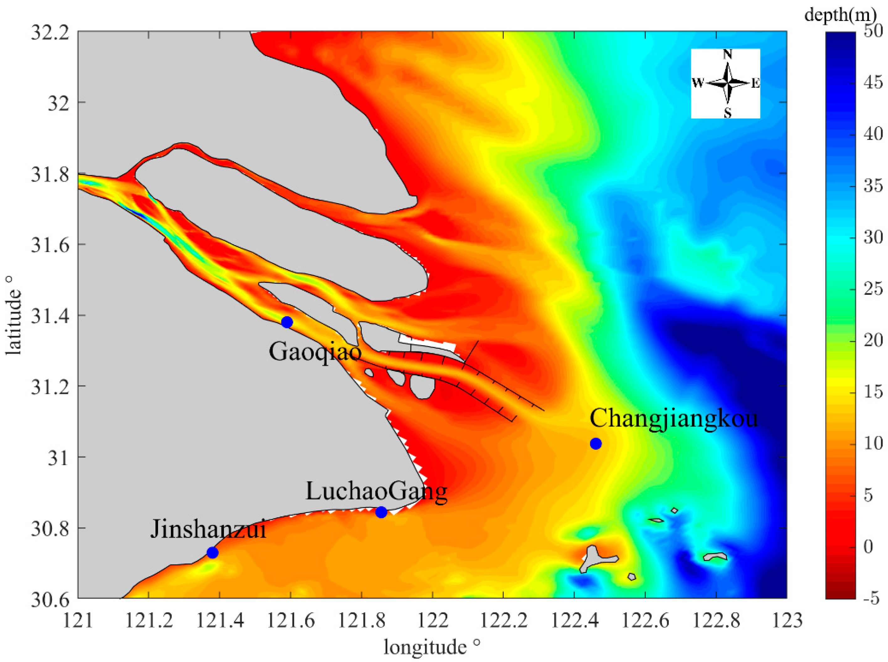
The Yangtze Estuary is the largest estuary in China (shown in Figure 1). Chongming Island separates the estuary into the North Branch and the South Branch. The North Channel and the South Channel are divided by Changxing Island and Hengsha Island. The Jiuduansha Shoal separates the South Channel into the North Passage and the South Passage. The ECMWF wind field data for the Yangtze Estuary were taken as the research object in this paper. Correlation analysis of the wind data between observed data and ECWMF reanalysis data was carried out in the Yangtze Estuary. A linear regression correction method for different underlying surfaces was proposed. The results were applied to the two-dimensional hydrodynamic model of the Yangtze River estuary to simulate the water level setup. The effects of the wind field on the model simulation results, before and after correction, were investigated.
2. Materials and Methods
2.1. ECMWF Reanalysis Wind Data and Correction Method
ERA-interim wind data were employed as the reanalysis wind data, with a spatial resolution of 0.125° (latitude) × 0.125° (longitude). As shown in Figure 2, the domain of reanalysis wind data covers the entire Yangtze Estuary and Hangzhou Bay. The wind speed and pressure at the height of ten meters above mean sea level are used at the time interval of 6 h, that is, at 0:00, 6:00, 12:00, and 18:00 GMT, every day. The duration of the reanalysis data is from 2014 to 2015. The observed wind data in 2014 at four stations were used to assess the quality of the reanalysis wind data. The measured wind data are supported by Shanghai Flood Risk Information Center. The locations of the 4 wind stations in the Yangtze Estuary have different characteristics: Gaoqiao station is located inside the estuary, which is constrained by the channel bank. Jinshanzui and Luchaogang stations are located on the north bank of the Hangzhou Bay, and the land is on their northerly and westerly sides. Changjiangkou station is located outside the estuary with a homogeneous underlying surface.
The correction method proposed by Mazaheri et al. allowed us to simply apply linear regression to obtain the modification factor of the wind components, including u and v. Based on the modification factors at every single station, the modification factors at each wind field grid point were obtained using interpolation. However, Wang’s research has pointed out that the underlying surface has a significant influence on the performance of wind correction. The wind correction method for the reanalysis data was proposed considering the different underlying surfaces in this research. First, we established a linear regression relationship between the direction of measured and reanalysis wind, which was used to modify the reanalysis wind direction. Then, the measured wind speed was divided into eight groups according to different wind directions in order to take different underlying surfaces into consideration: N–NE (0–45°), NE–E (45–90°), E–SE (90–135°), SE–S (135–180°), S–SW (180–225°), SW–W (225–270°), W–NW (270–315°), and NW–N (315–360°). The linear regression relationship between the observations of wind speed and reanalysis wind speed data in each group was obtained. Wind speed linear regression equations were also used to modify the reanalysis wind speed.
After the above processes, the difference between the measured and reanalysis wind data could be obtained. Due the effect that a single station’s distance can have, we used inverse distance weight interpolation with an influence radius [17] to modify the wind field.
In Equation (1), represents the weight of the physical information, such as wind speed and direction. represents the distance between the reanalysis wind data sample and the ith weather station. R denotes the influence radius. It means that the error only has an impact on the area under the influence radius. The impact at the wind station is the maximum and decays along the radius. In Equation (2), represents the modified wind data, represents the original reanalysis wind data, and denotes the error between the modified and original data in a single station.
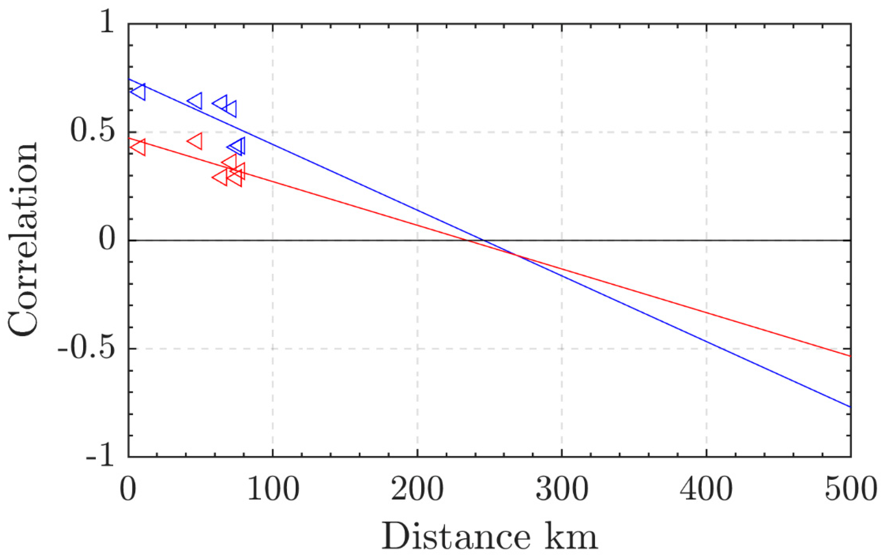
The correlation coefficients (CCs) of ERA-interim reanalysis data error between stations were analyzed to determine the influence radius, R. According to Yao’s research, the CC of wind data error shows a negative correlation with distance. The distance is the influence radius when the CC is 0. As shown in Figure 2, due to the distances between the 4 stations being less than 100 km, the CCs are all positive. The linear fitting is used to fit the distances and CCs. R-squared of wind velocity and direction is 0.5393 and 0.5224, respectively. Based on the distribution of CCs and distances, the influence radius, R, is 210 km in this research.
After a single station’s wind data are corrected, the wind field data are modified by Equations (1) and (2). The deviation between original and corrected reanalysis data is distributed in the weight of Wi to each grid point in the wind field within the influence radius.
In order to evaluate the corrected wind data quantitatively, error indices, including mean error (ME), root mean square error (RMSE) and skill scores (SSs) [18], are calculated as follows:
Herein, S represents the reanalysis value, O represents the measured value, n represents the number of samples used for calculation, and superscript represents the average of data. The following groups are classified based on SS > 0.65, indicating an excellent agreement with measured data; SS is between 0.5 and 0.65, which suggests a very good agreement with the observed data; the SS value of 0.2–0.5 suggests a good validation; if the value is less than 0.2, the model performance is poor.
2.2. Numerical Hydrodynamic Model
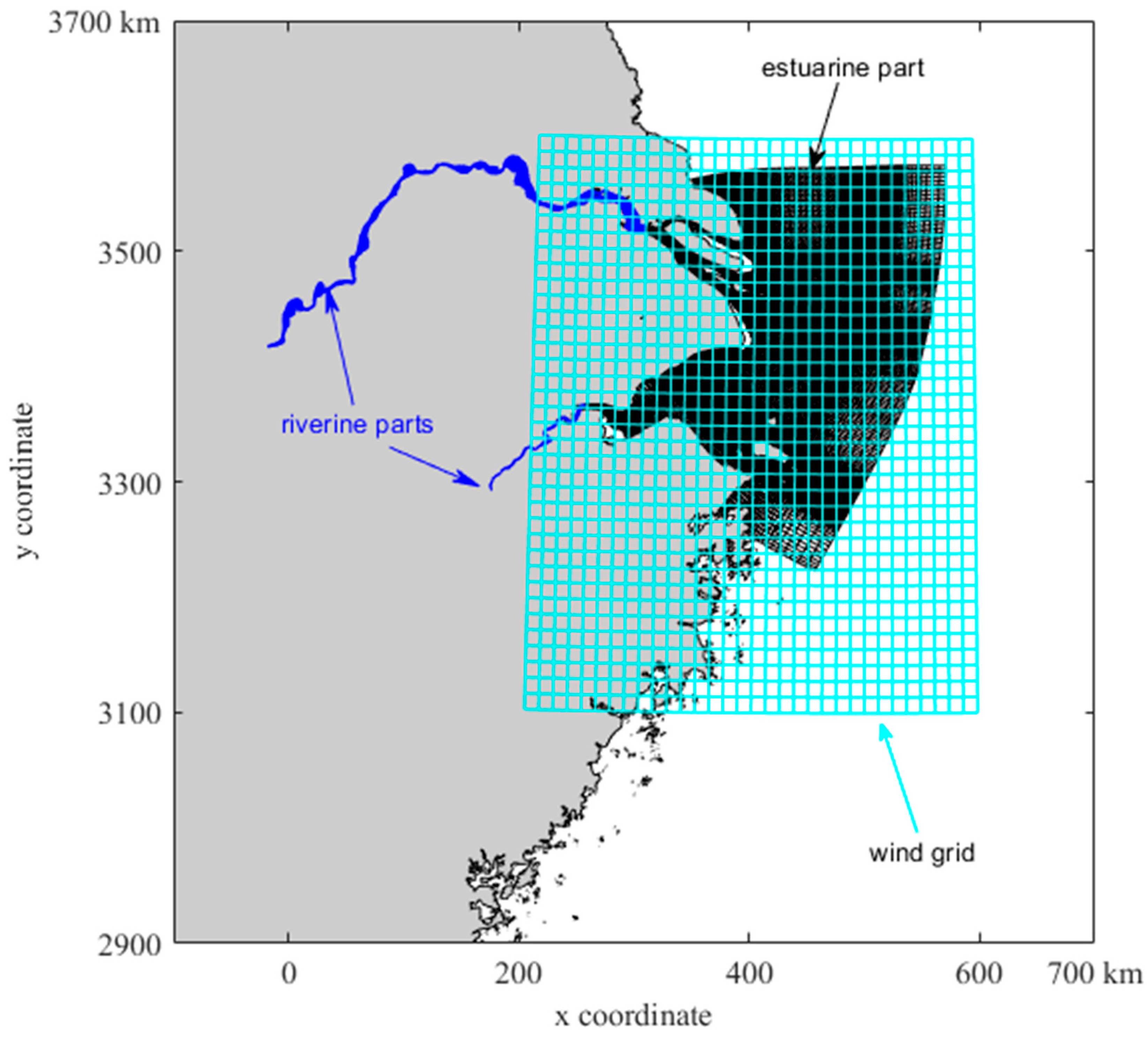
The calibrated and validated process-based model for the Yangtze Estuary based on Delft3D was used in this study to simulate the water level [6,19,20]. The flow model domain extends over about 800 km in the longitudinal direction and about 400 km in the lateral direction. It covers the entire Yangtze Estuary, Hangzhou Bay, and their adjacent seas (shown in Figure 3). The model is separated into three parts for computational efficiency: The Yangtze River, from Datong to Xuliujing, has 1056 grid nodes along the river and 30 points in the transverse direction, with a resolution varying from 100 m to 1.5 km. The Qiantang River, from Lucipu to Haining, has 137 grid nodes along the river and 6 points in the transverse direction, with a resolution varying from 200 m to 1.2 km. The estuary and adjacent coast cover a 300 km × 300 km area. This grid contains 200 × 200 grid nodes with a higher resolution near the river boundary and lower resolution near the sea boundary. The resolution of the estuary grid varies from 200 m to 6 km.
The daily mean discharge at Datong station and the monthly mean discharge at Lucipu station were provided as upstream boundary conditions. Tidal evaluation at open boundaries is represented by the mean sea level and 13 tidal constituents (M2, S2, N2, K2, K1, O1, P1, Q1, M.F., MM, M4, MS4, and MN4). The wind data used in the model were derived from ERA-interim data, and the wind was only applied to the sea domain. The bed friction coefficient is a key parameter that determines the bed shear stress and the distribution of the velocity field. The Manning coefficient was chosen to represent the bottom roughness in the model. A value of 0.019 s/m1/3 was applied in the riverine part, and 0.011 s/m1/3 was used in the estuarine part. The computational time step was selected as 1 min.
3. Results
3.1. Modified Single Station’s Wind Data
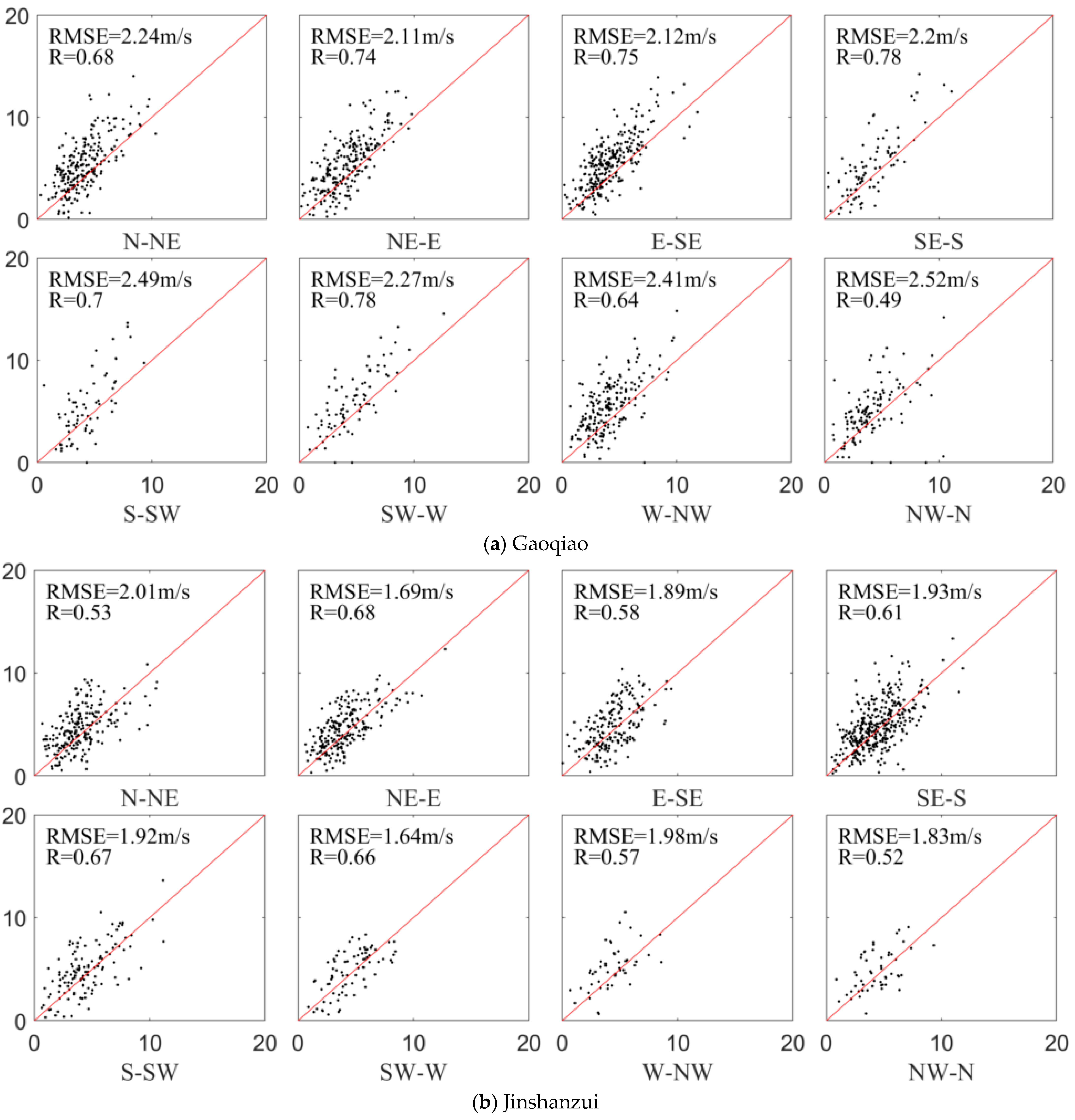
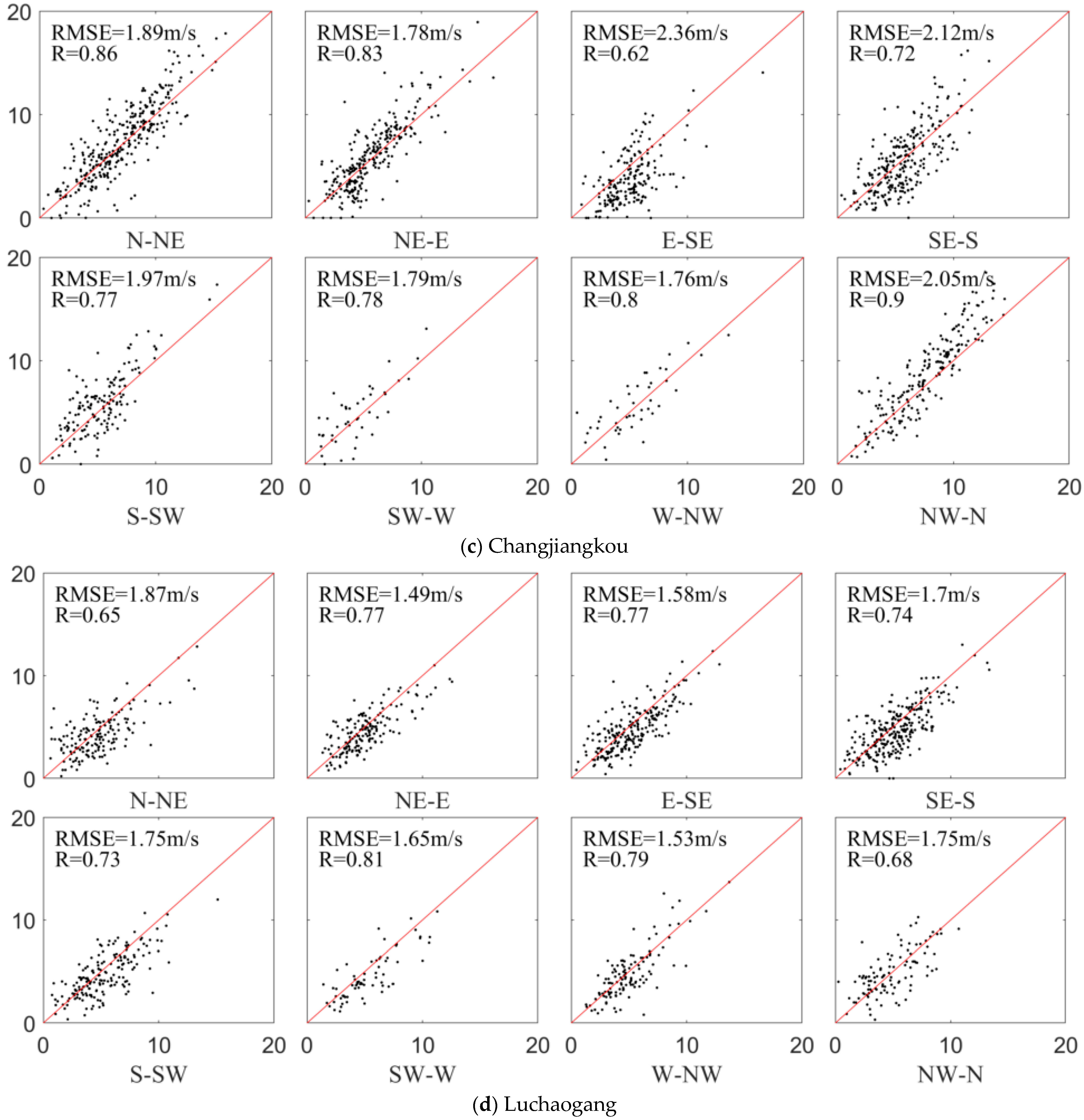
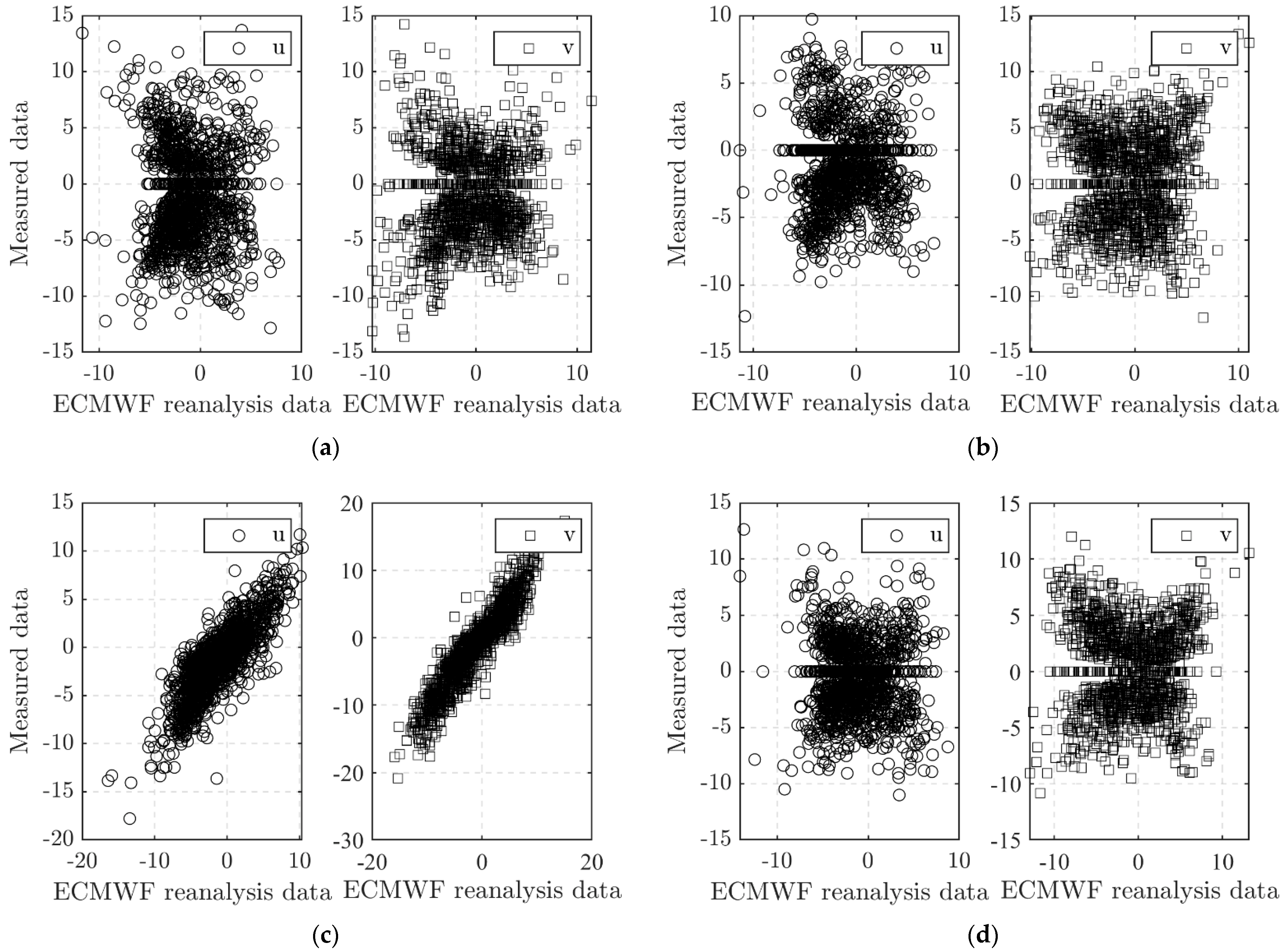
Figure 4 shows the comparison between measured and reanalysis wind speeds for the year 2014 in different directions at the four wind stations. The root mean square error at each station is within the range of 1.02–3.30 m/s, and the correlation coefficient, r, is within the range of 0.41–0.89. Therefore, high correlations between two types of wind data can be observed, confirming the feasibility of the linear regression method for wind modification.
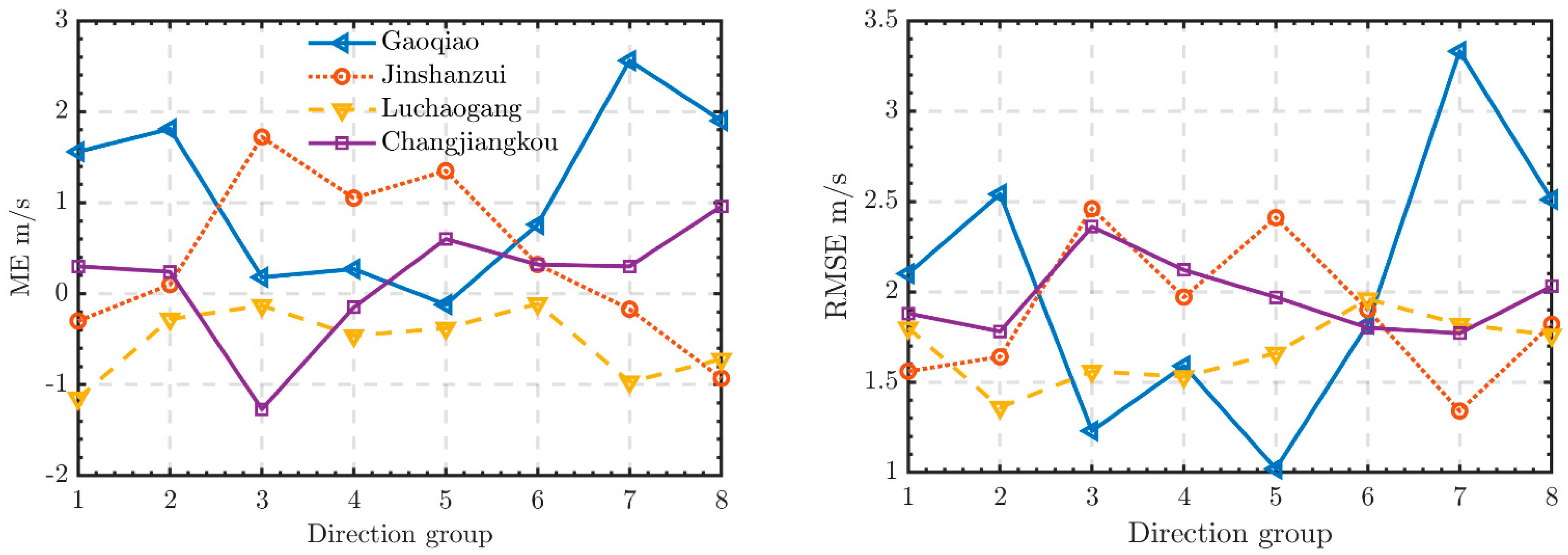
Previous research has shown that reanalysis data underestimate the intensity of tropical cyclones. However, the results of this research show a different finding. The wind speed obtained from the ERA-interim data does not show the underestimation of the actual wind speed for all the stations. Figure 5 shows the error of the reanalysis wind data compared to the observation at stations in the Yangtze Estuary in 2014. Only at Gaoqiao station was the reanalysis wind speed lower than the measured wind speed. The MEs of Gaoqiao station are between 0.12 and 0.27 m/s, and the RMSEs are between 1.02 and 3.33 m/s. The reason for this could be the location of the Gaoqiao station, which is located inside the Yangtze Estuary. The reanalysis wind magnifies the influence of the land underlying surface during data assimilation. The main channel of the estuary is in the NW–SE direction, resulting in the underestimation of reanalysis data in the direction from E to W.
Luchaogang station is located on the eastern side of Shanghai. The MEs are negative in all directions, indicating that the reanalysis data overestimate the measured data. The maximum ME is 1.15 m/s in the N–NE direction group. The reanalysis data cannot capture the characteristic of different underlying surface types near the shoreline due to its resolution. In the SW–N direction toward Luchaogang station, the underlying surface is a landform with a water surface in the other directions. As a consequence, the wind speed has a larger deviation in the W–NE direction group.
Jinshanzui station is located inside Hangzhou Bay. Its topographic effect is more significant than that of Luchaogang station. The wind speed is overestimated in the SW–NE direction and underestimated in the other directions.
Changjiangkou station is located outside the estuary, with little impact from the land’s underlying surface. The MEs in all directions were within the range of 0.15–0.96 m/s except for that in the E–SE direction. The small islands are on the south-eastern side of Changjiangkou, which could lead to the overestimation of the wind speed in the E–SE direction.
3.2. Validation of the Numerical Model
The model has previously been validated in the Yangtze Estuary and is shown to be capable of simulating water level, circulation, and salinity in the Yangtze Estuary. Here, more details on the performance of the model during the period of the winter season in 2017 are present when measured data are available.
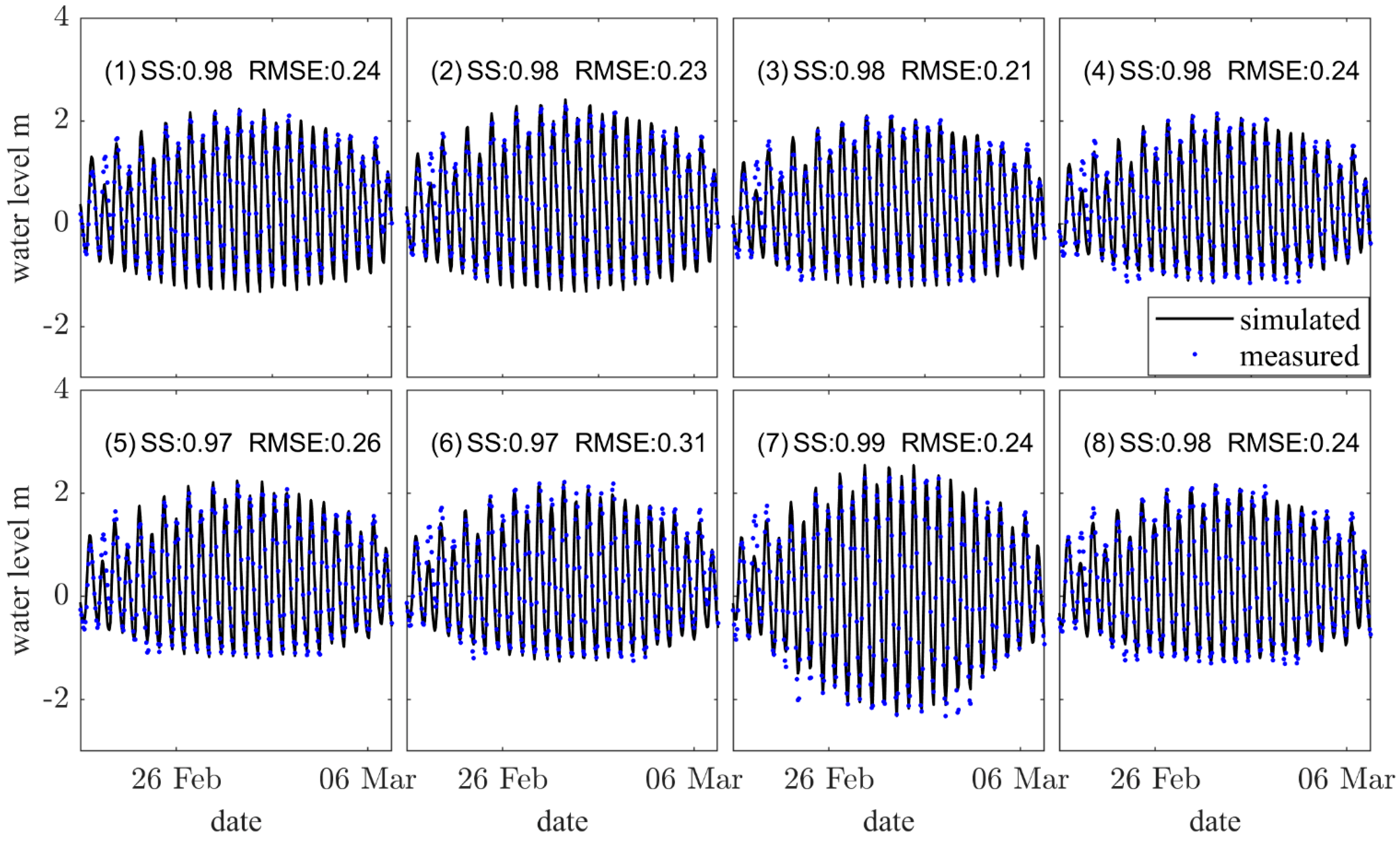
There are eight tide stations and eight current stations installed inside the estuary, which measure the water level and vertical profiles of current and salinity. The validation results are shown in Figure 6, Figure 7 and Figure 8. Overall, the model reproduced the water levels well in the Yangtze Estuary. All the SSs of water level at the stations are more than 0.96 during the simulation period.
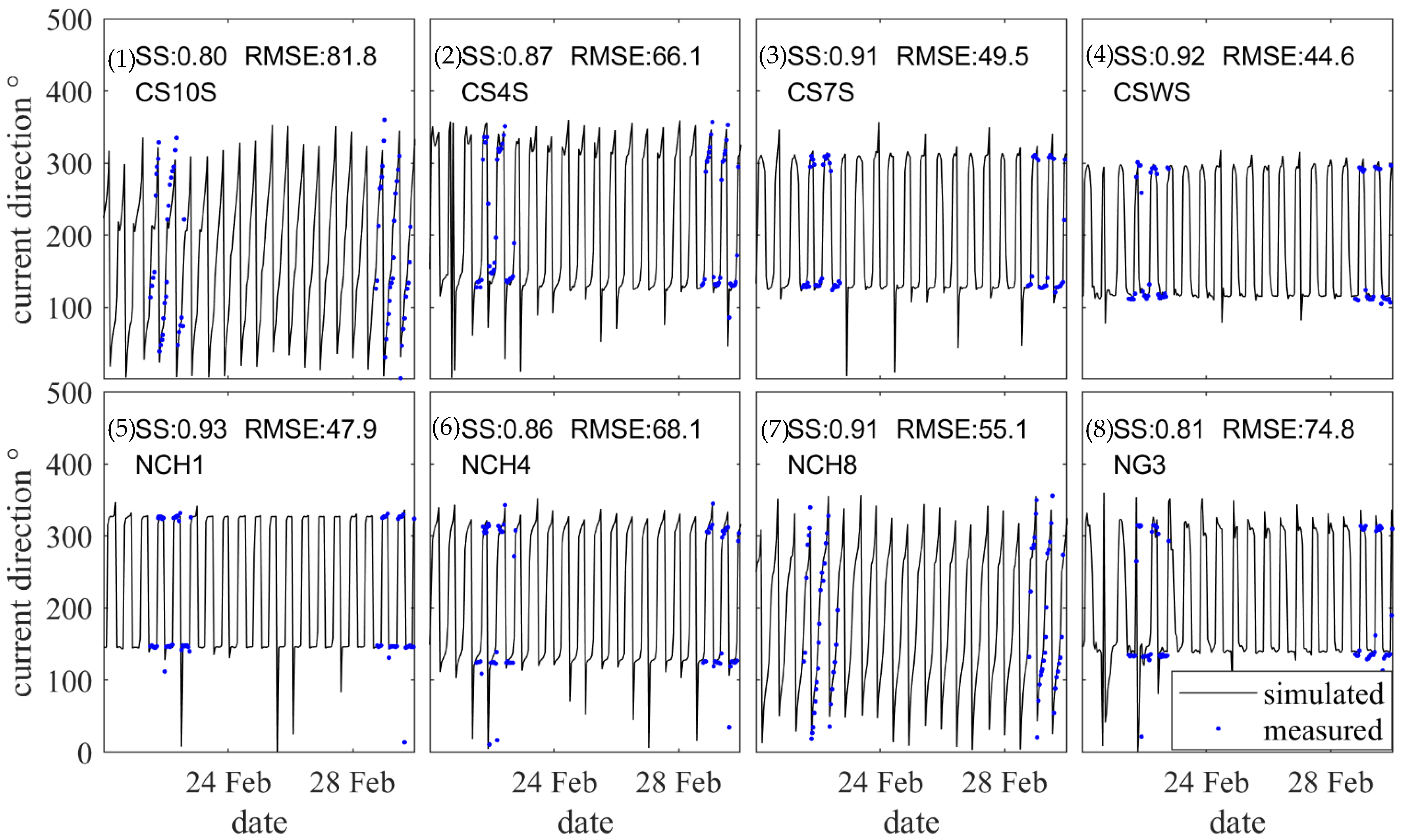
Figure 7 and Figure 8 show a comparison of the depth-averaged current velocity and direction between the observation and model results. Although the SS is lower than that for the water level, the agreement between the model and measurements is satisfactory and reasonable.
Overall, the model provides reasonable and acceptable water level and current simulations in the Yangtze Estuary. It can be applied in the further simulation of water level setup.
4. Discussion
4.1. Modified ERA-Interim Reanalysis Wind Data
As shown in Figure 4, there is a robust linear relationship between the reanalysis wind data and the measured wind data. The wind direction was modified by directly establishing the linear regression equation, and the wind speed was modified in the different wind direction groups. Table 1 shows the wind direction correction relationships for each station, where dire represents the direction of reanalysis data and dirr denotes the modified wind direction.
The wind speed correction equations are similar to the wind direction correction method in the following form: velr = a × vele + b, where velr is the modified wind speed, vele is the reanalysis wind speed, and a and b are coefficients. Table 2 shows the coefficients of wind speed correction equations for wind directions at each station. Modification factors of Mazaheri’s wind correction method for each station were also tested. However, excluding Changjiangkou station, the stations failed to obtain a reasonable modification factor (see Figure 9). Changjiangkou station is surrounded by the same underlying surface. There is an evident relationship between these observations and the reanalysis data. The other stations are influenced by different underlying surfaces. Mazaheri’s wind correction method is not suitable for the complex conditions in estuarine areas.
The measured wind data in 2015 were used to verify the effectiveness of the correction method. The deviations between the reanalysis data and the measured values were calculated before and after the correction. First, the reanalysis wind direction was modified by the linear relationship with the coefficient shown in Table 1. Then, classified by the modified wind direction, the linear regression method with the coefficient shown in Table 2 was applied in each direction group. The results are shown in Table 3. After the correction, the MEs and RMSEs of the wind direction at Gaoqiao and Jinshanzui stations decreased. However, an increase in MEs and RMSEs at Luchaogang station could be observed. The reason for this may be the difference in the wind direction at Luchaogang station between 2014 and 2015.
For wind speed, the MEs of the three stations decreased from 1.22 m/s, 0.62 m/s, 0.39 m/s to −0.05 m/s, 0.04 m/s and 0.02 m/s, respectively, and the RMSEs decreased from 1.68 m/s, 1.45 m/s, 1.27 m/s to 1.34 m/s, 1.25 m/s and 1.13 m/s, respectively, which indicates that the linear wind speed correction method with different wind direction has a good correction effect.
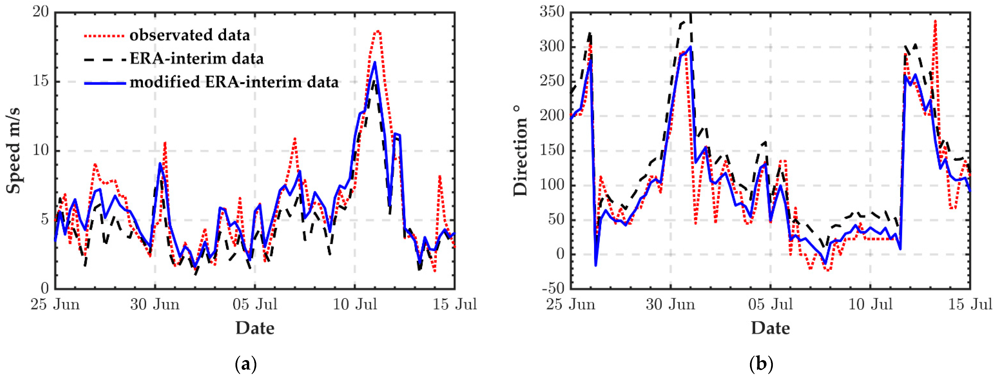
The modified wind speeds and directions at Gaoqiao station in July 2015 were compared with the observed data, as shown in Figure 10. The agreement of wind speed and direction between the modified ERA-interim data and observational data was significantly improved.
4.2. Application of Modified ERA-Interim Reanalysis Wind Data in the Estuary
To test the performance of modified ERA-interim reanalysis wind data in the water level hindcast, the ERA-interim wind and the modified ERA-interim wind were applied to drive the Yangtze Estuary flow model in order to simulate the water level during Typhoon Phenix.
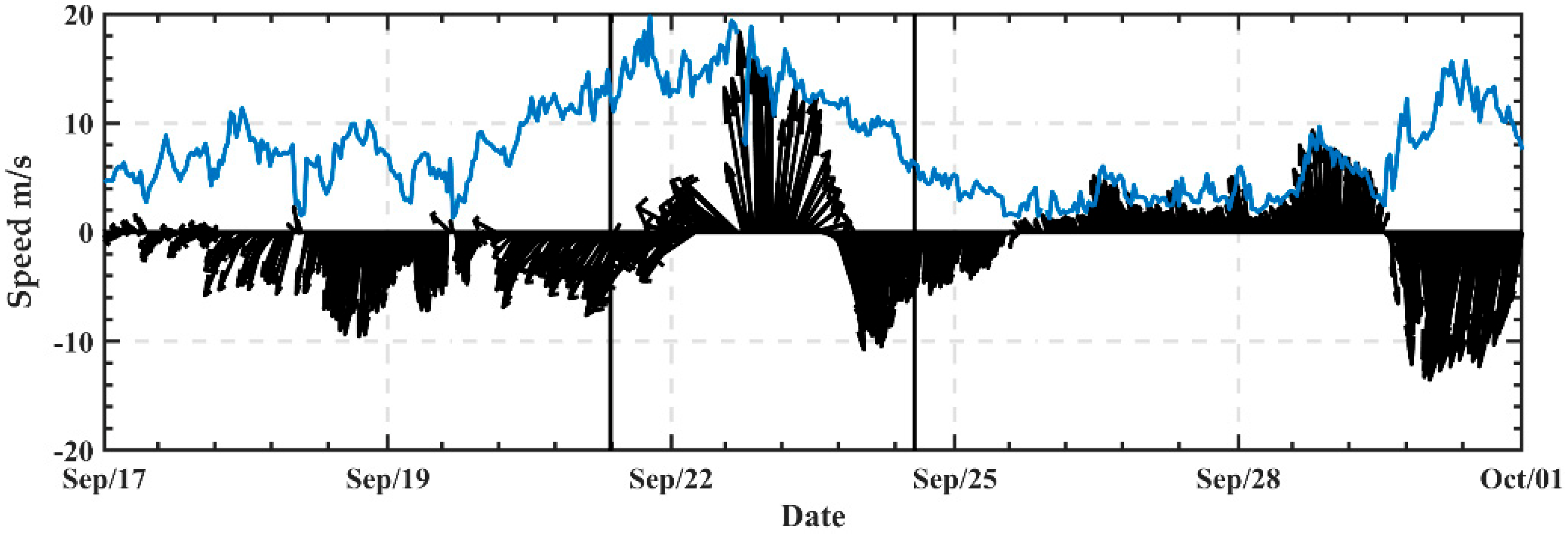
Typhoon Phoenix landed near the Yangtze River estuary on 22 September 2014. The maximum wind speed near the center was about 20 m/s, and the minimum air pressure at the center was 995 Pa. Figure 11 shows the wind speed at Changjiangkou station during the Typhoon Phoenix period. The original reanalysis data and the corrected wind field data were adopted in the numerical model to investigate the wind quality after the correction.
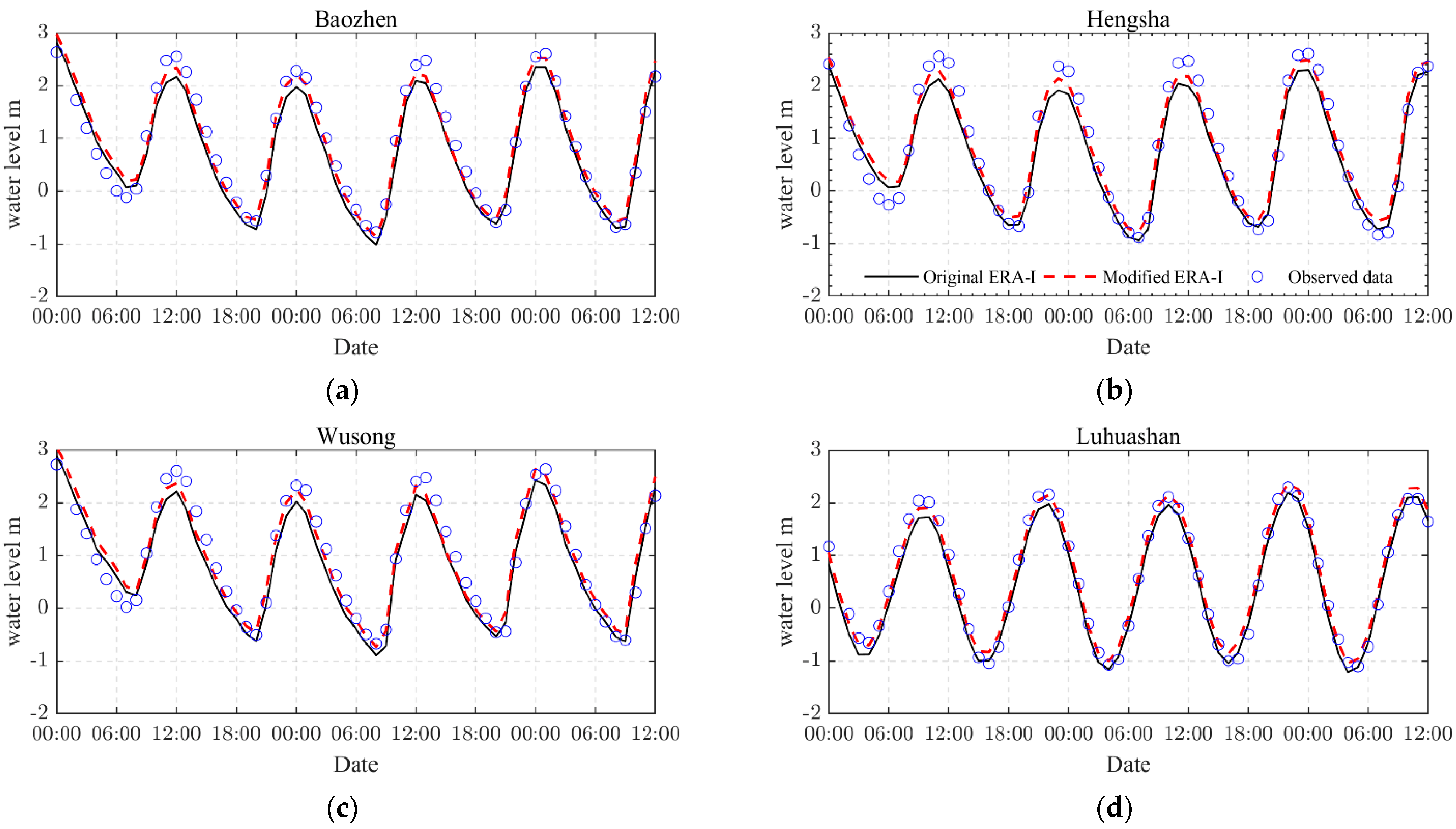
Figure 12 shows the observed water levels against those simulated under different wind conditions at the four stations in the Yangtze Estuary. The statistics of the errors in the measured and simulated water levels before and after the application of the modified winds are shown in Table 4. Although the errors in the ME and RMSE at Luhuashan station increased, the errors in the other stations displayed a visible decrease. The skill scores at all stations increased, indicating that the modified wind improved the water level simulation performance. High water level (HWL) is the characteristic water level of concern in coastal protection. The simulated high water levels were about 28 cm, 38 cm, 30 cm, and 18 cm lower than those observed at Baozhen, Hengsha, Wusong, and Luhuashan stations, respectively. By applying the corrected reanalysis wind data, the simulated highest water level was consistent with the observations. The deviations in high water level at the four stations were about 12 cm, 21 cm, 13 cm and 1 cm. It is noted that this application only focuses on the wind-induced water setup. Previous research proposed that the radius of maximum winds and the wave-induced water setup have a significant effect on the simulation of storm surges [21,22]. The purpose of this research is to propose a wind correction method suitable for estuarine areas. Applying the correction method proposed in this paper to reanalysis wind data can improve the accuracy of simulated water levels in the Yangtze Estuary during typhoons.
5. Conclusions
In this paper, the correlation between ERA-interim wind data and measured wind data in the Yangtze Estuary was analyzed. A modification method considering different underlying surface influences was proposed, with linear regression for a single station and inverse distance weight interpolation for a spatial wind field. The modified wind field was used to drive a two-dimensional hydrodynamic model for the Yangtze River estuary in order to simulate the water levels under typhoon conditions.
The results show that the proposed linear correction method of wind speed at stations with different underlying surfaces can significantly improve the agreement between reanalysis wind data and measured wind data. After the wind field was corrected, by using the inverse distance weight interpolation method, the accuracy of simulated high water levels under typhoon conditions could be significantly improved. This study provides useful guidance on the modification of reanalysis wind data for the simulation of storm surges in the Yangtze Estuary. With more measured data becoming available, the correction method can be further improved.
Author Contributions
Conceptualization, Y.C. (Yongping Chen); methodology, A.C.; software, M.G.; data curation, Z.T. and M.G.; writing—original draft preparation, Z.T.; writing—review and editing, S.P.; visualization, Y.C. (Yuhang Chen); supervision, A.C.; funding acquisition, Z.T., Z.C. and Y.Z. All authors have read and agreed to the published version of the manuscript.
Funding
This research was funded by the Fundamental Research Funds for the Central Universities of China (B200204017), the Postgraduate Research & Practice Innovation Program of Jiangsu Province (KJCX21_0526) and the Fundamental Research Program for Public Welfare of Zhejiang Province (LGF22D060010).
Institutional Review Board Statement
Not applicable.
Informed Consent Statement
Not applicable.
Data Availability Statement
The data presented in this study are available on request from the corresponding author. The data are not publicly available because the raw/processed data required to reproduce these findings cannot be shared at this time as the data also form part of an ongoing study.
Conflicts of Interest
The authors declare no conflict of interest.
References
- Hu, K.; Ding, P.; Ge, J. Modelling of Storm Surge in the Coastal Waters of Yangtze Estuary and Hangzhou Bay, China. J. Coast. Res. 2007, 8, 527–533. [Google Scholar]
- Wang, Y.; Gao, T.; Han, Z.; Liu, Q. Impacts of Wind-Field Correction on the Numerical Simulation of Storm-Surge Inundation during Typhoon “Rammasun”. Estuar. Coast. Shelf Sci. 2017, 196, 198–206. [Google Scholar] [CrossRef]
- Kwon, Y.-Y.; Choi, J.-W.; Kwon, J.-I. Simulation of Storm Surge Due to the Changes of Typhoon Moving Speed in the South Coast of Korean Peninsula. J. Coast. Res. 2020, 95, 1467–1472. [Google Scholar] [CrossRef]
- He, Z.; Tang, Y.; Xia, Y.; Chen, B.; Xu, J.; Yu, Z.; Li, L. Interaction Impacts of Tides, Waves and Winds on Storm Surge in a Channel-Island System: Observational and Numerical Study in Yangshan Harbor. Ocean Dyn. 2020, 70, 307–325. [Google Scholar] [CrossRef]
- Li, L.; Zhu, J.; Chant, R.J.; Wang, C.; Pareja-Roman, L.F. Effect of Dikes on Saltwater Intrusion Under Various Wind Conditions in the Changjiang Estuary. J. Geophys. Res. Oceans 2020, 125, e2019JC015685. [Google Scholar] [CrossRef]
- Tao, Z.; Chu, A.; Chen, Y.; Lu, S.; Wang, B. Wind Effect on the Saltwater Intrusion in the Yangtze Estuary. J. Coast. Res. 2020, 105, 42–46. [Google Scholar] [CrossRef]
- Lai, W.; Pan, J.; Devlin, A.T. Impact of Tides and Winds on Estuarine Circulation in the Pearl River Estuary. Cont. Shelf Res. 2018, 168, 68–82. [Google Scholar] [CrossRef]
- Song, D.; Wang, X.H. Suspended Sediment Transport in the Deepwater Navigation Channel, Yangtze River Estuary, China, in the Dry Season 2009: 2. Numerical Simulations. J. Geophys. Res. Oceans 2013, 118, 5568–5590. [Google Scholar] [CrossRef]
- Chen, L.; Gong, W.; Scully, M.E.; Zhang, H.; Cheng, W.; Li, W. Axial Wind Effects on Stratification and Longitudinal Sediment Transport in a Convergent Estuary During Wet Season. J. Geophys. Res. Oceans 2020, 125, e2019JC015254. [Google Scholar] [CrossRef]
- Lv, X.; Yuan, D.; Ma, X.; Tao, J. Wave Characteristics Analysis in Bohai Sea Based on ECMWF Wind Field. Ocean Eng. 2014, 91, 159–171. [Google Scholar] [CrossRef]
- Li, J.; Chen, Y.; Pan, S.; Pan, Y.; Fang, J.; Sowa, D.M.A. Estimation of Mean and Extreme Waves in the East China Seas. Appl. Ocean Res. 2016, 56, 35–47. [Google Scholar] [CrossRef]
- Zhang, Y.-Q. Evaluation of three reanalysis surface wind products in Taiwan Strait. J. Fish. Res. 2020, 42, 556–571. (In Chinese) [Google Scholar]
- Cavaleri, L.; Sclavo, M. The Calibration of Wind and Wave Model Data in the Mediterranean Sea. Coast. Eng. 2006, 53, 613–627. [Google Scholar] [CrossRef]
- Yang, X.; He, J.; Lv, J.; Wang, Y.; He, Q. Impacts of the Sea—Level Wind Field Correction on the Numerical Simulation of Storm Surges. Meteorol. Mon. 2011, 37, 270–275. (In Chinese) [Google Scholar]
- Bajo, M.; Zampato, L.; Umgiesser, G.; Cucco, A.; Canestrelli, P. A Finite Element Operational Model for Storm Surge Prediction in Venice. Estuar. Coast. Shelf Sci. 2007, 75, 236–249. [Google Scholar] [CrossRef]
- Mazaheri, S.; Kamranzad, B.; Hajivalie, F. Modification of 32 years ECMWF wind field using QuikSCAT data for wave hindcasting in Iranian Seas. J. Coast. Res. 2005, 65 Pt 1, 344–349. [Google Scholar] [CrossRef]
- Yao, R.; Tu, X.; Ding, Y.; Wang, W.; Wu, F.; Zhu, A. Verification and Correction on ASCAT Wind Velocities Within the Offshore East Chian Sea. Acta Meteorol. Sin. 2015, 26, 735–742. (In Chinese) [Google Scholar]
- Willmott, C.J. On the Validation of Models. Phys. Geogr. 1981, 2, 184–194. [Google Scholar] [CrossRef]
- Chu, A.; Wang, Z.B.; de Vriend, H.J. Process-Based Modeling for the Yangtze Estuary. In Proceedings of the Coastal Dynamics 2009, Tokyo, Japan, 7–11 September 2009; World Scientific: Tokyo, Japan, 2009; pp. 1–13. [Google Scholar]
- Chu, A.; Wang, Z.B.; de Vriend, H. Analysis on Residual Coarse Sediment Transport in Estuaries. Estuar. Coast. Shelf Sci. 2015, 163, 194–205. [Google Scholar] [CrossRef]
- Kim, S.Y.; Yasuda, T.; Mase, H. Wave setup in the storm surge along open coasts during Typhoon Anita. Coast. Eng. 2010, 57, 631–642. [Google Scholar] [CrossRef]
- Li, Y.; Fang, W.H.; Lin, W.; Ye, Y.T. Parameterisation of synthetic tropical cyclones at various scales for probable maximum storm surge risk modeling. Mar. Sci. 2014, 38, 71–80. [Google Scholar]
Figure 1.
The bathymetry of Yangtze estuary and locations of wind stations.

Figure 2.
The distribution of CC of ERA-interim reanalysis data errors to station distances in 2014. (blue and red represent wind direction and velocity, respectively.).
Figure 2.
The distribution of CC of ERA-interim reanalysis data errors to station distances in 2014. (blue and red represent wind direction and velocity, respectively.).

Figure 3.
Grids of the reanalysis wind data and hydrodynamic model.

Figure 4.
Correlation of measured and ERA-interim wind speed with different directions at different stations. (a) Gaoqiao, (b) Jinshan, (c) Changjiangkou, and (d) Luchaogang (the horizontal axis is for the ERA-interim wind speed, the vertical axis is for the measured wind speed, and the unit is m/s).


Figure 5.
MEs and RMSEs in different directions at different stations. 1–8 represent N–NE, NE–E, E–SE, SE–S, S–SW, SW–W, W–NW, and NW–N, respectively.
Figure 5.
MEs and RMSEs in different directions at different stations. 1–8 represent N–NE, NE–E, E–SE, SE–S, S–SW, SW–W, W–NW, and NW–N, respectively.

Figure 6.
Model validation results for water level. (1–8), measured (blue dots) and simulated (black line) results at Baimao, Chongtou, Yanglin, Shidongkou, Wusong, Liuyao, Lianxinggang, and Hengsha, respectively.
Figure 6.
Model validation results for water level. (1–8), measured (blue dots) and simulated (black line) results at Baimao, Chongtou, Yanglin, Shidongkou, Wusong, Liuyao, Lianxinggang, and Hengsha, respectively.

Figure 7.
Model validation results for current velocity. (1–8), measured (blue dots) and simulated (black line) results at CS10S, CS4S, CS7S, CSWS, NCH1, NCH4, NCH8, and NG3, respectively.
Figure 7.
Model validation results for current velocity. (1–8), measured (blue dots) and simulated (black line) results at CS10S, CS4S, CS7S, CSWS, NCH1, NCH4, NCH8, and NG3, respectively.

Figure 8.
Model validation results for current direction. (1–8), measured (blue dots) and simulated (black line) results at CS10S, CS4S, CS7S, CSWS, NCH1, NCH4, NCH8, and NG3, respectively.
Figure 8.
Model validation results for current direction. (1–8), measured (blue dots) and simulated (black line) results at CS10S, CS4S, CS7S, CSWS, NCH1, NCH4, NCH8, and NG3, respectively.

Figure 9.
Sample scatter diagrams for wind vector components. (a) Gaoqiao, (b) Jinshanzui, (c) Changjiangkou, (d) Luchaogang.
Figure 9.
Sample scatter diagrams for wind vector components. (a) Gaoqiao, (b) Jinshanzui, (c) Changjiangkou, (d) Luchaogang.

Figure 10.
Comparisons between the ERA-interim, modified ERA-interim, and observational data of wind speed (a) and wind direction (b) in July 2015.
Figure 10.
Comparisons between the ERA-interim, modified ERA-interim, and observational data of wind speed (a) and wind direction (b) in July 2015.

Figure 11.
Measured wind data at Changjiangkou station in September 2014, where the period of Typhoon Phoenix is indicated by two vertical lines.
Figure 11.
Measured wind data at Changjiangkou station in September 2014, where the period of Typhoon Phoenix is indicated by two vertical lines.

Figure 12.
Water level comparison before and after correction at each station during Typhoon Phoenix in September. (a) Baozhen, (b) Hengsha, (c) Wusong, (d) Luhuashan.
Figure 12.
Water level comparison before and after correction at each station during Typhoon Phoenix in September. (a) Baozhen, (b) Hengsha, (c) Wusong, (d) Luhuashan.


Table 1.
Correction equations of wind direction at each station.
| Stations | Modified Relation |
|---|---|
| Gaoqiao | |
| Jinshanzui | |
| Luchaogang | |
| Changjiangkou |
Table 2.
Coefficients of corrections equations of wind speed at stations.
| Stations | Gaoqiao | Jinshanzui | Luchaogang | Changjiangkou | ||||
|---|---|---|---|---|---|---|---|---|
| Coefficients | a | b | a | b | a | b | a | b |
| N–NE | 0.96 | 1.70 | 0.65 | 1.39 | 0.80 | 0.08 | 1.04 | 0.05 |
| NE–E | 0.67 | 3.15 | 0.66 | 1.64 | 0.87 | 0.38 | 1.03 | 0.07 |
| E–SE | 0.85 | 0.79 | 0.89 | 2.19 | 0.75 | 1.03 | 0.76 | −0.03 |
| SE–S | 0.78 | 1.08 | 0.78 | 1.98 | 0.62 | 1.33 | 0.95 | 0.15 |
| S–SW | 0.71 | 0.93 | 0.90 | 1.69 | 0.68 | 1.11 | 0.97 | 0.74 |
| SW–W | 0.93 | 1.05 | 0.62 | 1.48 | 0.62 | 1.35 | 0.93 | 0.62 |
| W–NW | 1.18 | 1.63 | 1.23 | −1.15 | 0.67 | 0.89 | 0.82 | 1.28 |
| NW–N | 0.99 | 1.94 | 0.37 | 1.97 | 0.70 | 0.92 | 1.15 | −0.13 |
Table 3.
Comparison of wind direction and speed errors of each station before and after correction.
| Error Indices | ME | RMSE | |||
|---|---|---|---|---|---|
| Station | Original | Modified | Original | Modified | |
| Wind direction | Gaoqiao | −32.60 | −1.87 | 41.79 | 26.94 |
| Jinshanzui | 30.78 | −0.65 | 42.37 | 28.86 | |
| Luchaogang | −10.32 | −31.45 | 27.81 | 38.82 | |
| Wind speed | Gaoqiao | 1.22 | −0.05 | 1.68 | 1.34 |
| Jinshanzui | 0.62 | −0.04 | 1.45 | 1.25 | |
| Luchaogang | −0.39 | 0.02 | 1.27 | 1.13 | |
Table 4.
Statistics of errors in measured and simulated water levels before and after application of the modified winds.
Table 4.
Statistics of errors in measured and simulated water levels before and after application of the modified winds.
| ME | RMSE | SS | Deviation of HWL (Unit: m) | |||||
|---|---|---|---|---|---|---|---|---|
| Stations | Original | Modified | Original | Modified | Original | Modified | Original | Modified |
| Baozhen | 0.096 | −0.065 | 0.28 | 0.26 | 0.977 | 0.98 | 0.286 | 0.106 |
| Hengsha | 0.091 | −0.063 | 0.298 | 0.281 | 0.976 | 0.979 | 0.379 | 0.2 |
| Wusong | 0.126 | −0.038 | 0.309 | 0.282 | 0.969 | 0.974 | 0.3 | 0.112 |
| Luhuashan | 0.011 | −0.135 | 0.694 | 0.703 | 0.892 | 0.893 | 0.187 | 0.007 |
Publisher’s Note: MDPI stays neutral with regard to jurisdictional claims in published maps and institutional affiliations. |
© 2022 by the authors. Licensee MDPI, Basel, Switzerland. This article is an open access article distributed under the terms and conditions of the Creative Commons Attribution (CC BY) license (https://creativecommons.org/licenses/by/4.0/).
Share and Cite
MDPI and ACS Style
Tao, Z.; Chen, Y.; Chu, A.; Pan, S.; Gan, M.; Chen, Y.; Che, Z.; Zhu, Y. The Modified Method of Reanalysis Wind Data in Estuarine Areas. Water 2022, 14, 1826. https://doi.org/10.3390/w14111826
AMA Style
Tao Z, Chen Y, Chu A, Pan S, Gan M, Chen Y, Che Z, Zhu Y. The Modified Method of Reanalysis Wind Data in Estuarine Areas. Water. 2022; 14(11):1826. https://doi.org/10.3390/w14111826
Chicago/Turabian StyleTao, Zhengjin, Yongping Chen, Ao Chu, Shunqi Pan, Min Gan, Yuhang Chen, Zhumei Che, and Ye Zhu. 2022. "The Modified Method of Reanalysis Wind Data in Estuarine Areas" Water 14, no. 11: 1826. https://doi.org/10.3390/w14111826
Note that from the first issue of 2016, this journal uses article numbers instead of page numbers. See further details here.