
Using Stable Water Isotopes to Analyze Spatiotemporal Variability and Hydrometeorological Forcing in Mountain Valley Wetlands

 , and
, and 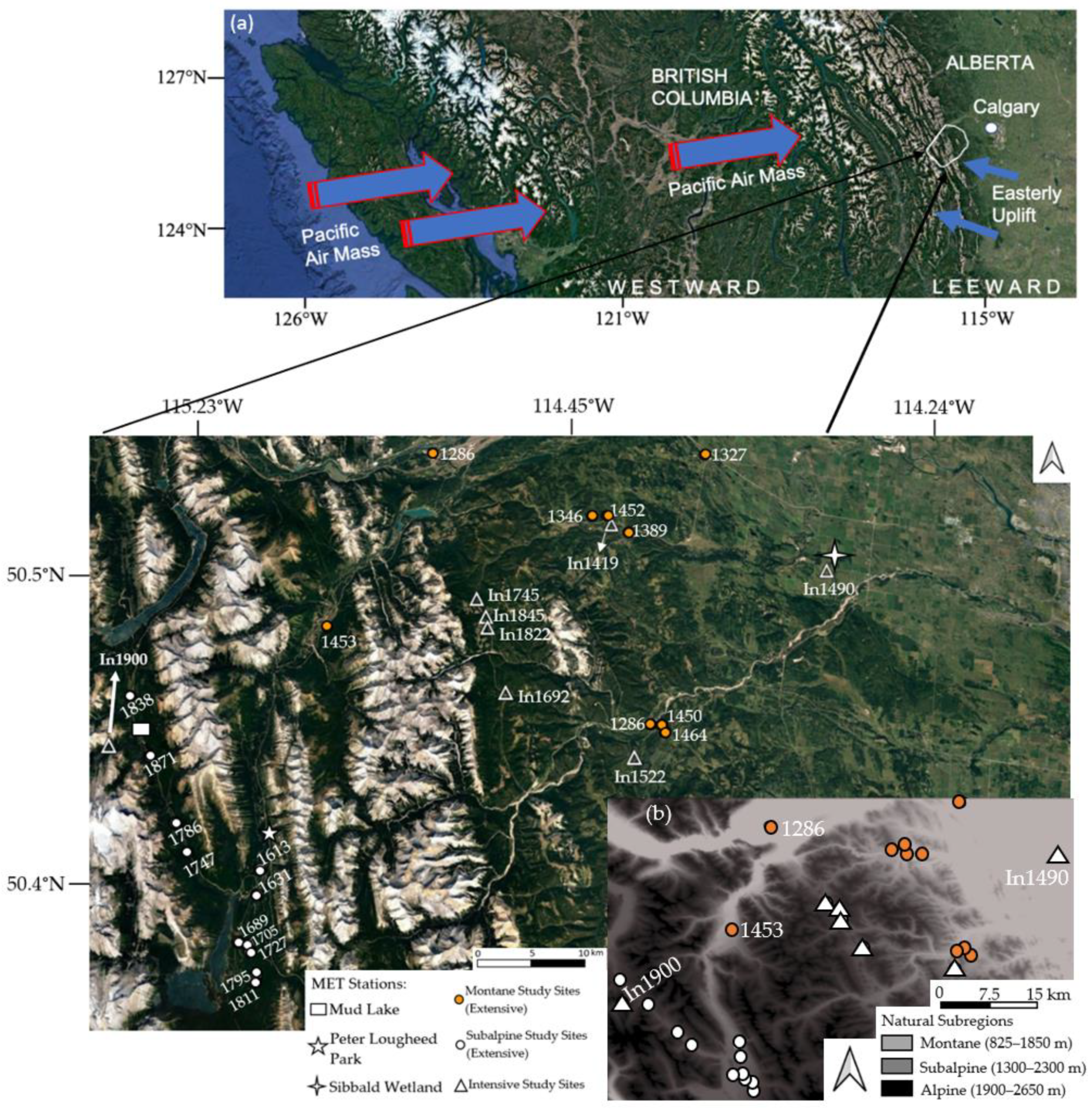
Abstract
:1. Introduction
2. Materials and Methods
2.1. Study Site Description
2.2. Wetland Identification
2.3. Isotope Data Collection
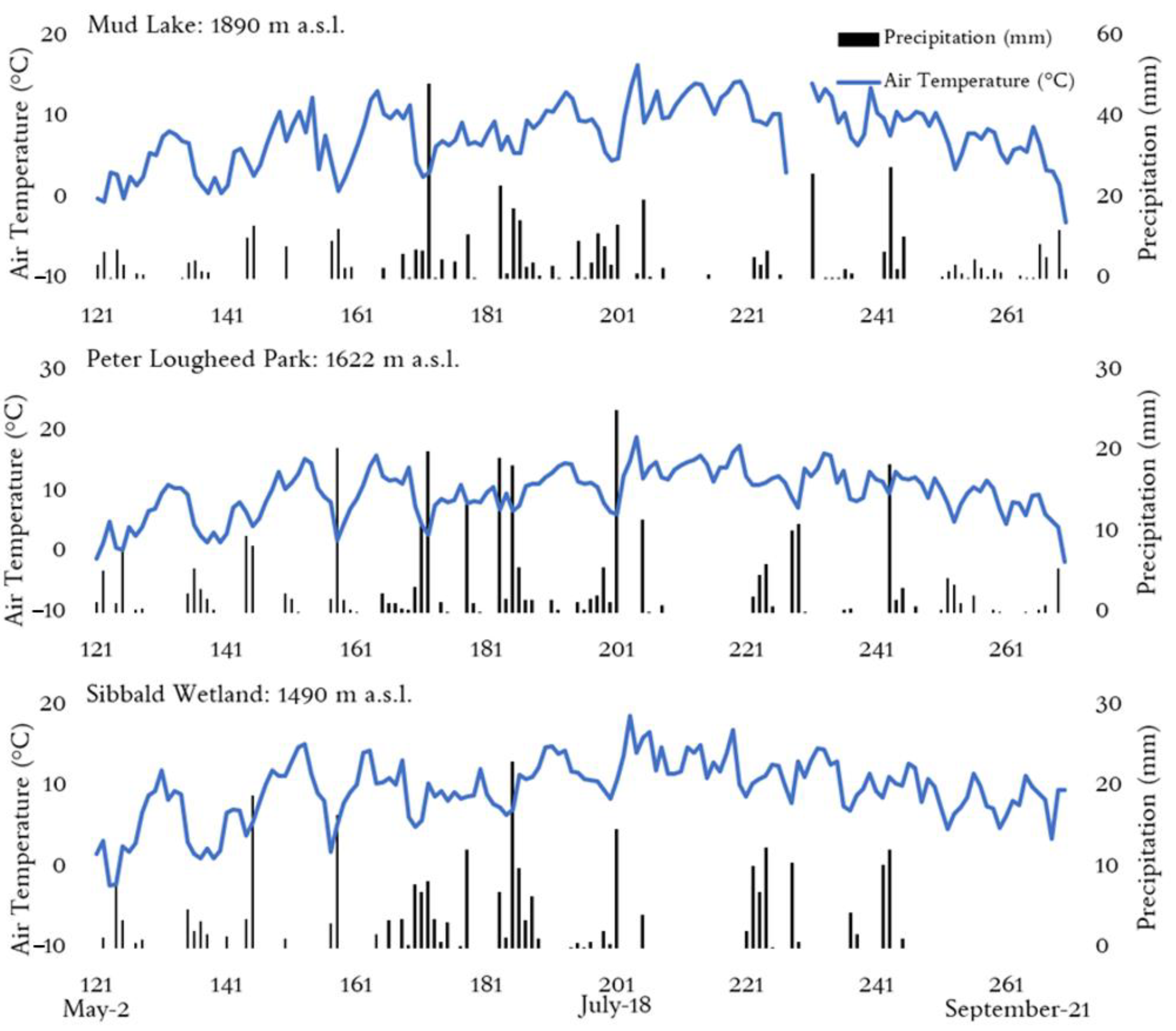
2.4. Meteorological Data
2.5. Data Analysis
3. Results
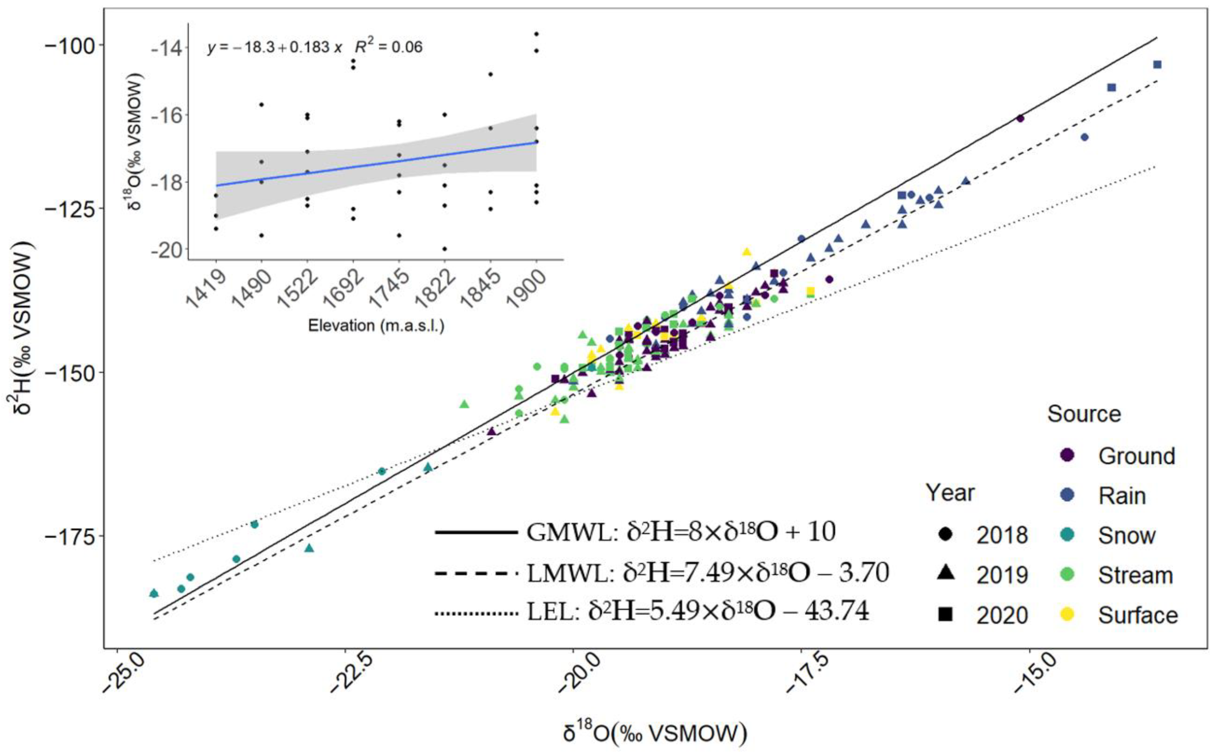
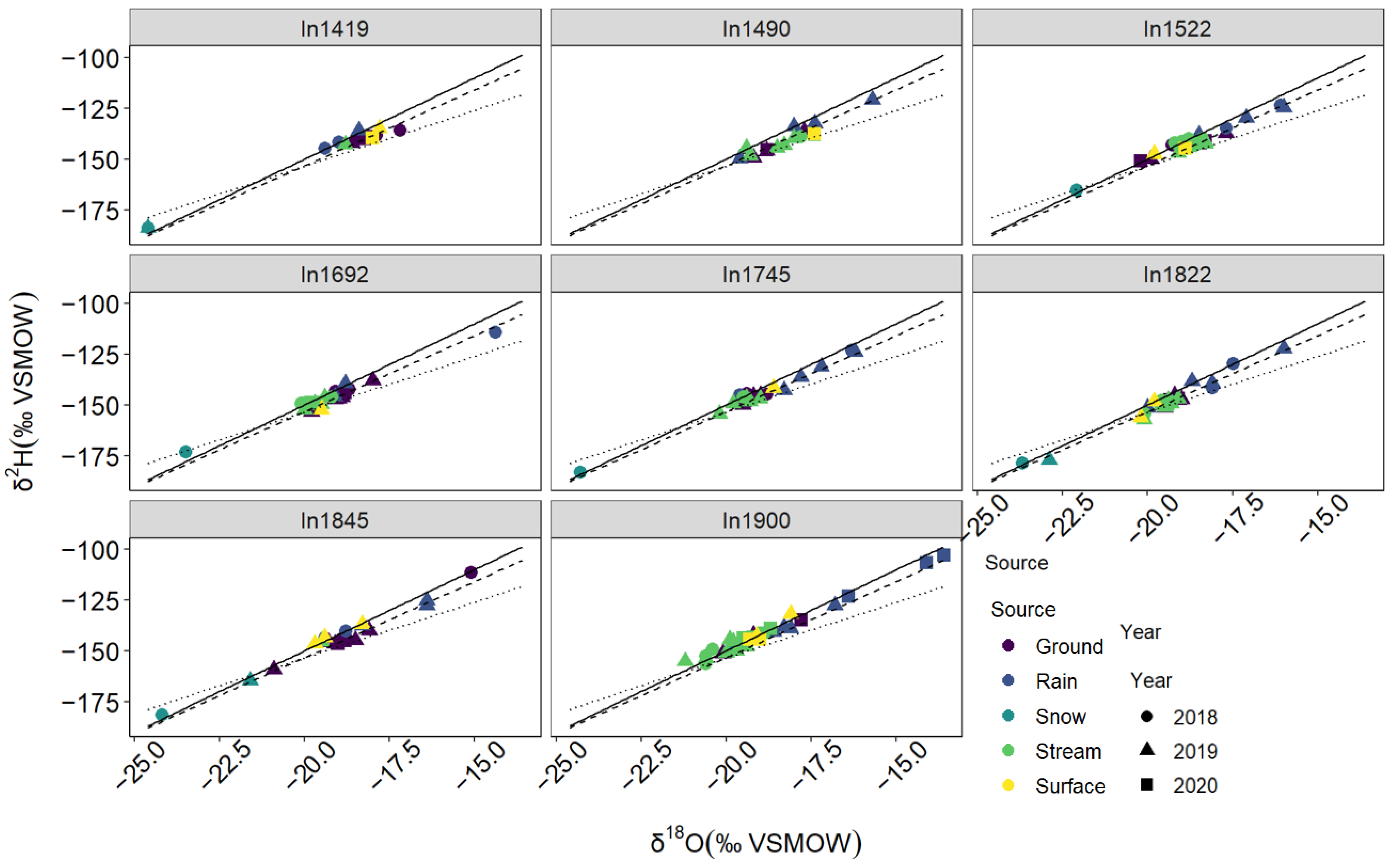
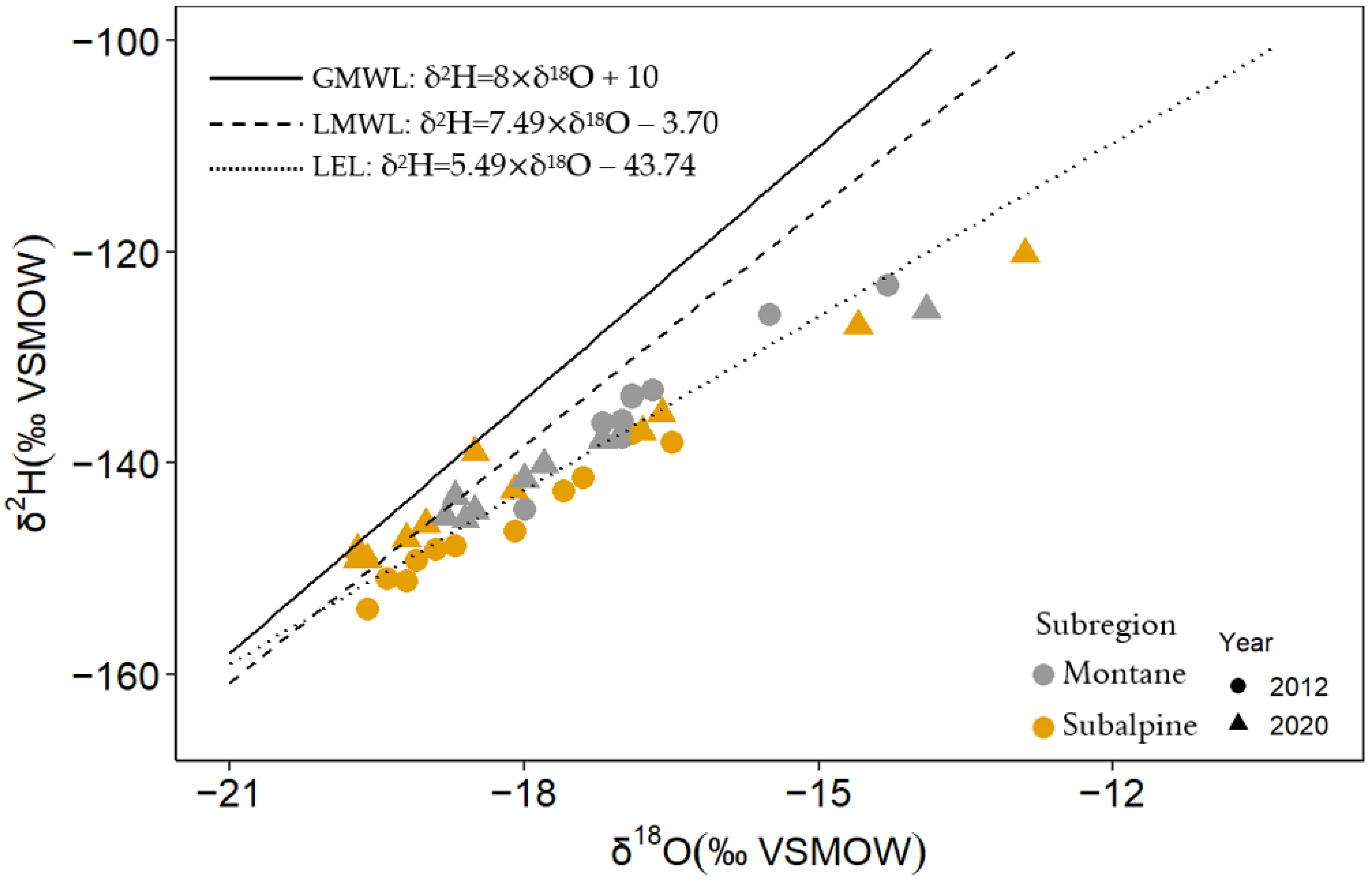
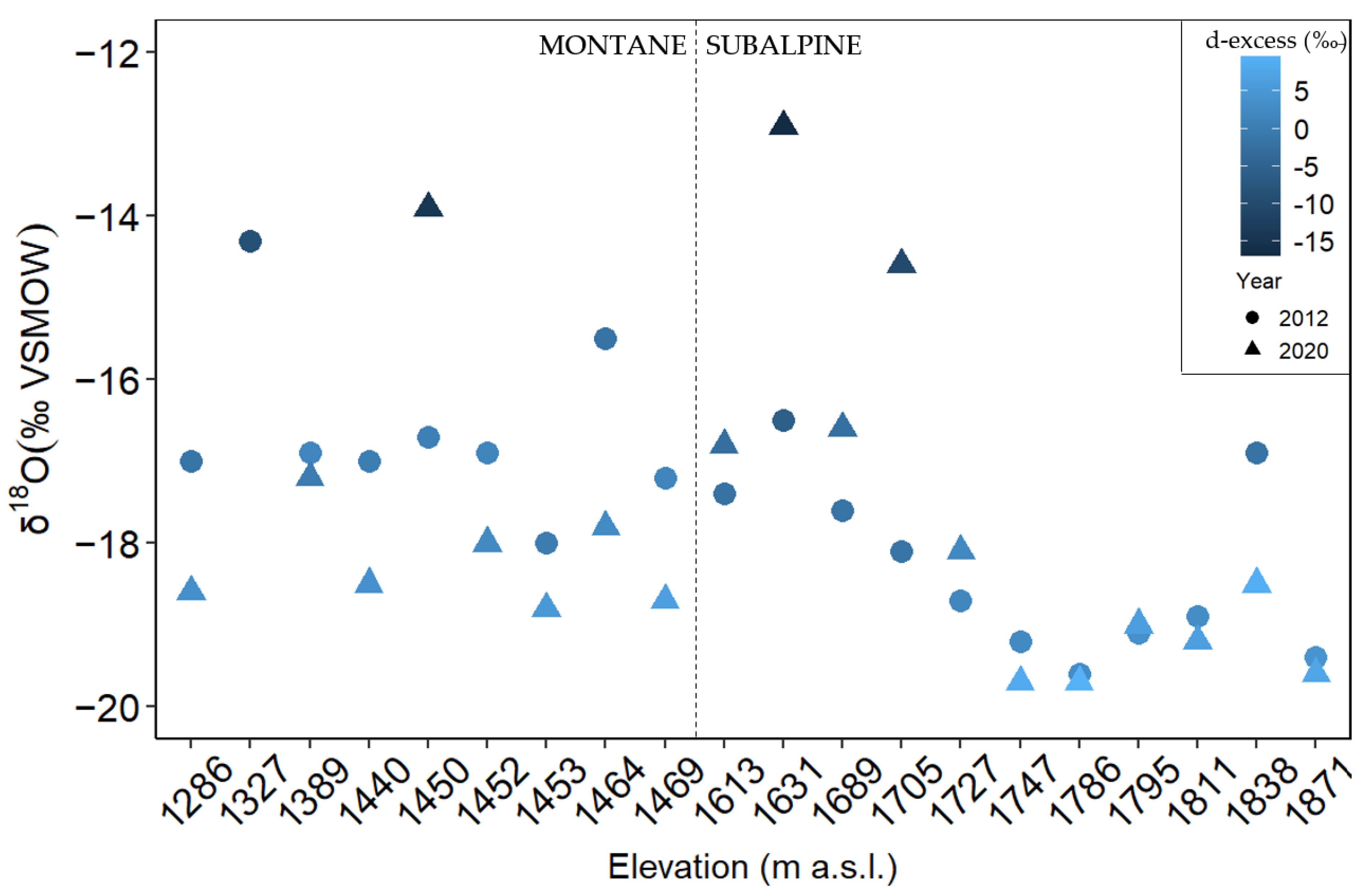
3.1. Spatial Variability in Isotopes
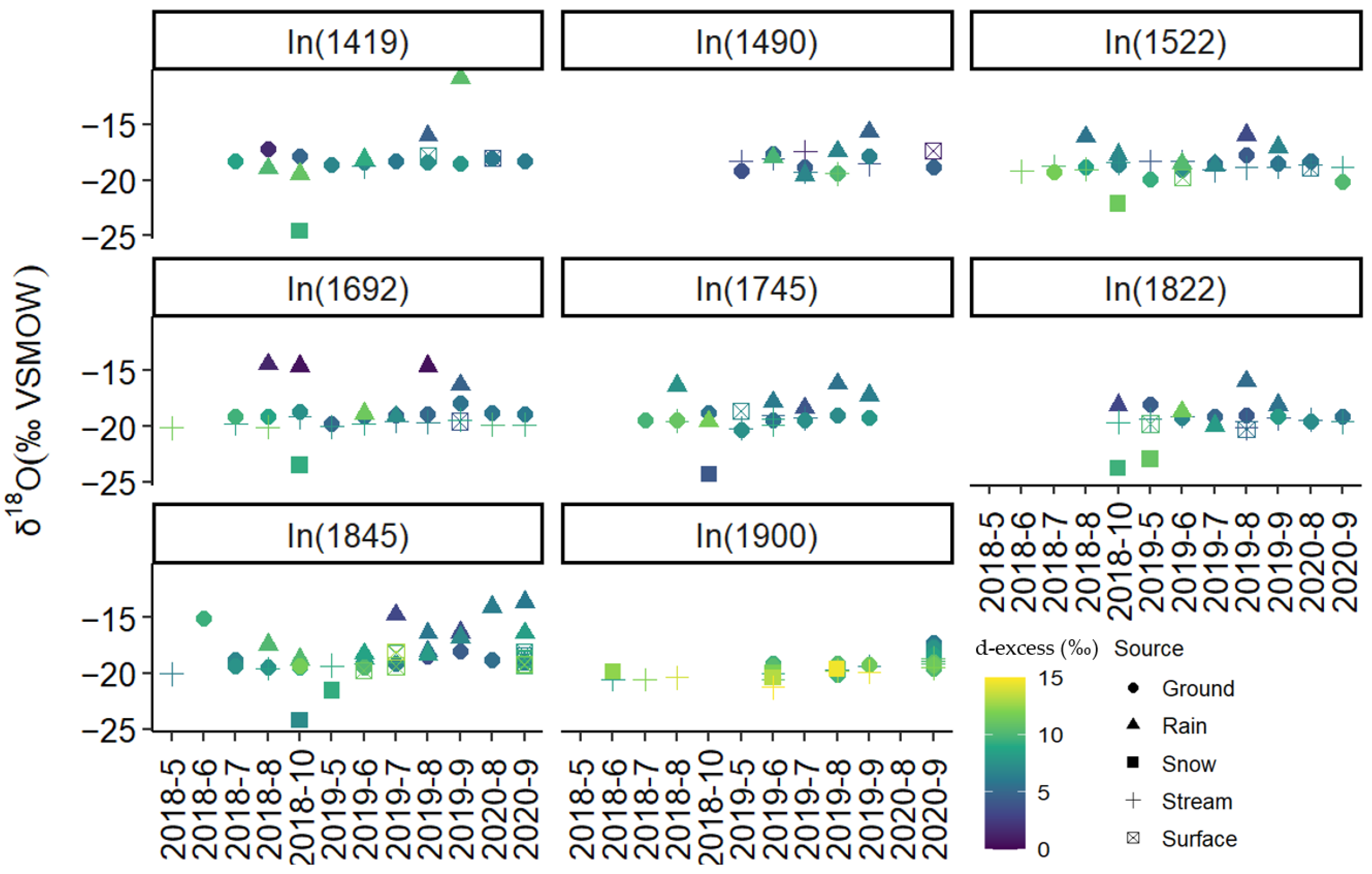
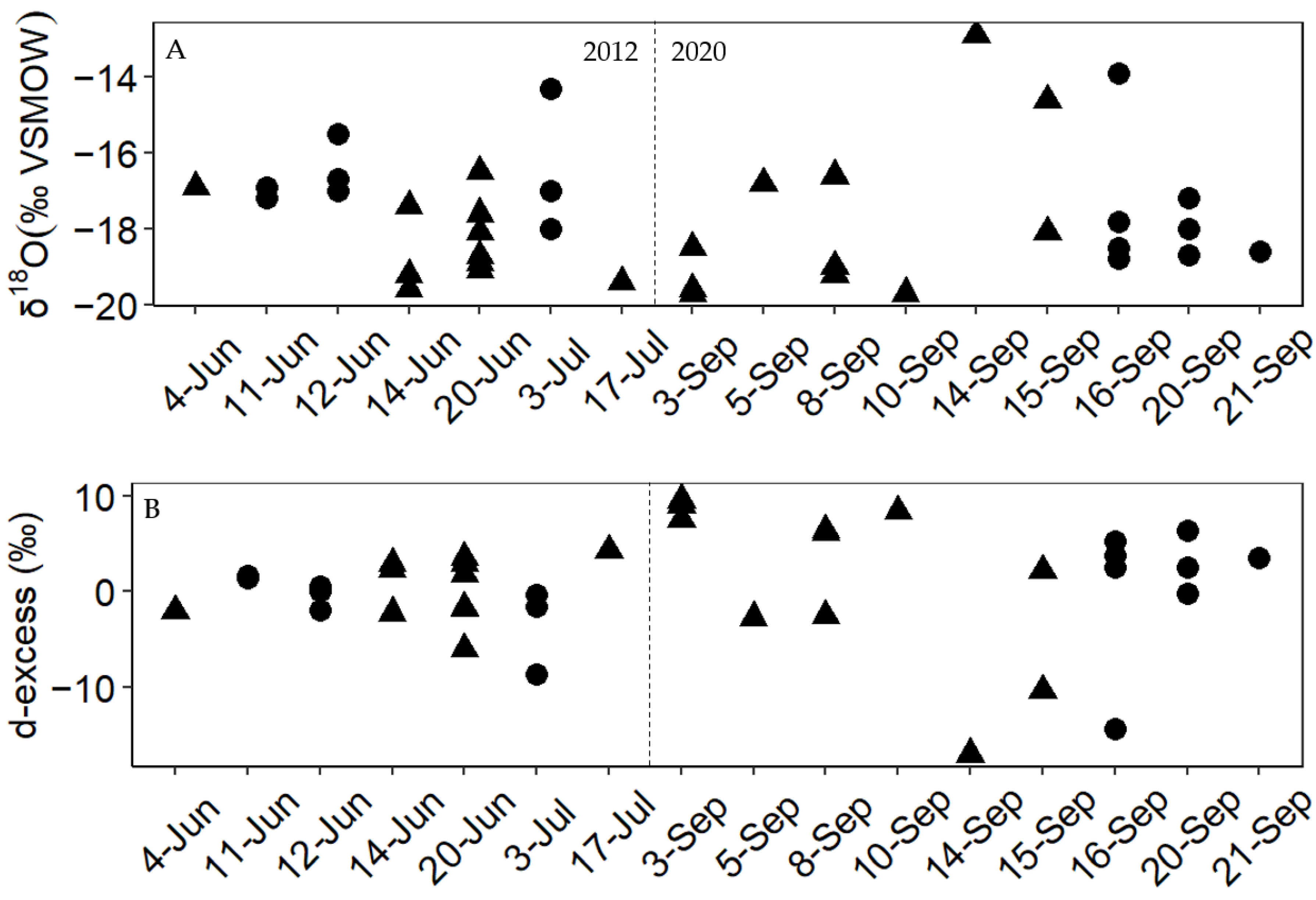
3.2. Temporal Variability in Isotopes
4. Discussion
4.1. Spatial Variability in Isotopes
4.2. Temporal Variability in Isotopes
4.3. Limitations and Future Work
5. Conclusions
Supplementary Materials
Author Contributions
Funding
Institutional Review Board Statement
Informed Consent Statement
Data Availability Statement
Acknowledgments
Conflicts of Interest
References
- Kadykalo, A.N.; Findlay, C.S. The flow regulation services of wetlands. Ecosyst. Serv. 2016, 20, 91–103. [Google Scholar] [CrossRef]
- Brooks, J.R.; Mushet, D.M.; Vanderhoof, M.K.; Leibowitz, S.G.; Christensen, J.R.; Neff, B.P.; Rosenberry, D.O.; Rugh, W.D.; Alexander, L.C. Estimating wetland connectivity to streams in the Prairie Pothole Region: An isotopic and remote sensing approach. Water Resour. Res. 2018, 54, 955–977. [Google Scholar] [CrossRef] [PubMed]
- Rangwala, I.; Miller, J.R. Climate change in mountains: A review of elevation-dependent warming and its possible causes. Clim. Chang. 2012, 114, 527–547. [Google Scholar] [CrossRef]
- Stewart, I.T. Changes in snowpack and snowmelt runoff for key mountain regions. Hydrol. Processes Int. J. 2009, 23, 78–94. [Google Scholar] [CrossRef]
- Pomeroy, J.W.; Stewart, R.E.; Whitfield, P.H. The 2013 flood event in the South Saskatchewan and Elk River basins: Causes, assessment and damages. Can. Water Resour. J. Rev. Can. Des Ressour. Hydr. 2016, 41, 105–117. [Google Scholar] [CrossRef]
- McDonnell, J.J.; Beven, K. Debates—The future of hydrological sciences: A (common) path forward? A call to action aimed at understanding velocities, celerities and residence time distributions of the headwater hydrograph. Water Resour. Res. 2014, 50, 5342–5350. [Google Scholar] [CrossRef]
- Dansgaard, W. Stable isotopes in precipitation. Tellus 1964, 16, 436–468. [Google Scholar] [CrossRef]
- Cui, J.; Tian, L.; Biggs, T.W.; Wen, R. Deuterium-excess determination of evaporation to inflow ratios of an alpine lake: Implications for water balance and modeling. Hydrol. Processes 2017, 31, 1034–1046. [Google Scholar] [CrossRef]
- Froehlich, K.; Kralik, M.; Papesch, W.; Rank, D.; Scheifinger, H.; Stichler, W. Deuterium excess in precipitation of Alpine regions–moisture recycling. Isot. Environ. Health Stud. 2008, 44, 61–70. [Google Scholar] [CrossRef]
- Whitfield, P.H. Climate station analysis and fitness for purpose assessment of 3053600 Kananaskis, Alberta. Atmos. Ocean 2014, 52, 363–383. [Google Scholar] [CrossRef]
- Craig, H. Standard for reporting concentrations of deuterium and oxygen-18 in natural waters. Science 1961, 133, 1833–1834. [Google Scholar] [CrossRef] [PubMed]
- Wassenaar, L.I.; Athanasopoulos, P.; Hendry, M.J. Isotope hydrology of precipitation, surface and ground waters in the Okanagan Valley, British Columbia, Canada. J. Hydrol. 2011, 411, 37–48. [Google Scholar] [CrossRef]
- Craig, H.; Gordon, L.I. Deuterium and Oxygen 18 Variations in the Ocean and the Marine Atmosphere, in Stable Isotopes in Oceanographic Studies and Palaeotemperatures, Spoleto 1965; Tongiorgi, E., Ed.; Consiglio Nazionale della Richerche: Pisa, Italy, 1965; pp. 9–130. [Google Scholar]
- Gat, J.R. Oxygen and hydrogen isotopes in the hydrologic cycle. Annu. Rev. Earth Planet. Sci. 1996, 24, 225–262. [Google Scholar] [CrossRef] [Green Version]
- Gibson, J.J.; Edwards, T.W.D.; Bursey, G.G.; Prowse, T.D. Estimating Evaporation Using Stable Isotopes: Quantitative Results and Sensitivity Analysis for Two Catchments in Northern Canada: Paper presented at the 9th Northern Res. Basin Symposium/Workshop (Whitehorse/Dawson/Inuvik, Canada-August 1992). Hydrol. Res. 1993, 24, 79–94. [Google Scholar] [CrossRef]
- Penna, D.; Engel, M.; Mao, L.; Dell’Agnese, A.; Bertoldi, G.; Comiti, F. Tracer-based analysis of spatial and temporal variations of water sources in a glacierized catchment. Hydrol. Earth Syst. Sci. 2014, 18, 5271–5288. [Google Scholar] [CrossRef] [Green Version]
- Carol, E.; Braga, F.; Da Lio, C.; Kruse, E.; Tosi, L. Environmental isotopes applied to the evaluation and quantification of evaporation processes in wetlands: A case study in the Ajó Coastal Plain wetland, Argentina. Environ. Earth Sci. 2015, 74, 5839–5847. [Google Scholar] [CrossRef]
- Ala-Aho, P.; Soulsby, C.; Pokrovsky, O.S.; Kirpotin, S.N.; Karlsson, J.; Serikova, S.; Vorobyev, S.N.; Manasypov, R.M.; Loiko, S.; Tetzlaff, D. Using stable isotopes to assess surface water source dynamics and hydrological connectivity in a high-latitude wetland and permafrost influenced landscape. J. Hydrol. 2018, 556, 279–293. [Google Scholar] [CrossRef]
- Shi, Y.; Jia, W.; Zhu, G.; Ding, D.; Yuan, R.; Xu, X.; Zhang, Z.; Yang, L.; Xiong, H. Hydrogen and Oxygen Isotope Characteristics of Water and the Recharge Sources in Subalpine of Qilian Mountains, China. Pol. J. Environ. Stud. 2021, 30, 2325–2339. [Google Scholar] [CrossRef]
- Semwal, P.; Khobragarde, S.; Joshi, S.K.; Kumar, S. Variation in δ18O and δ2H values of rainfall, surface water, and groundwater in the Sukhna Lake basin in northwest India. Environ. Earth Sci. 2020, 79, 1–14. [Google Scholar] [CrossRef]
- Marchina, C.; Lencioni, V.; Paoli, F.; Rizzo, M.; Bianchini, G. Headwaters’ isotopic signature as a tracer of stream origins and climatic anomalies: Evidence from the Italian Alps in summer 2018. Water 2020, 12, 390. [Google Scholar] [CrossRef] [Green Version]
- Shi, M.; Wang, S.; Argiriou, A.A.; Zhang, M.; Guo, R.; Jiao, R.; Kong, J.; Zhang, Y.; Qiu, X.; Zhou, S. Stable Isotope Composition in Surface Water in the Upper Yellow River in Northwest China. Water 2019, 11, 967. [Google Scholar] [CrossRef] [Green Version]
- Wu, H.; Wu, J.; Song, F.; Abuduwaili, J.; Saparov, A.S.; Chen, X.; Shen, B. Spatial distribution and controlling factors of surface water stable isotope values (δ18O and δ2H) across Kazakhstan, Central Asia. Sci. Total Environ. 2019, 678, 53–61. [Google Scholar] [CrossRef] [PubMed]
- Cao, X.; Wu, P.; Zhou, S.; Han, Z.; Tu, H.; Zhang, S. Seasonal variability of oxygen and hydrogen isotopes in a wetland system of the Yunnan-Guizhou Plateau, southwest China: A quantitative assessment of groundwater inflow fluxes. Hydrogeol. J. 2018, 26, 215–231. [Google Scholar] [CrossRef]
- Biggs, T.W.; Lai, C.T.; Chandan, P.; Lee, R.M.; Messina, A.; Lesher, R.S.; Khatoon, N. Evaporative fractions and elevation effects on stable isotopes of high elevation lakes and streams in arid western Himalaya. J. Hydrol. 2015, 522, 239–249. [Google Scholar] [CrossRef]
- Kumar, U.S.; Kumar, B.; Rai, S.P.; Sharma, S. Stable isotope ratios in precipitation and their relationship with meteorological conditions in the Kumaon Himalayas, India. J. Hydrol. 2010, 391, 1–8. [Google Scholar] [CrossRef]
- Gonfiantini, R.; Roche, M.A.; Olivry, J.C.; Fontes, J.C.; Zuppi, G.M. The altitude effect on the isotopic composition of tropical rains. Chem. Geol. 2001, 181, 147–167. [Google Scholar] [CrossRef]
- Mezga, K.; Urbanc, J.; Cerar, S. The isotope altitude effect reflected in groundwater: A case study from Slovenia. Isot. Environ. Health Stud. 2014, 50, 33–51. [Google Scholar] [CrossRef]
- Giustini, F.; Brilli, M.; Patera, A. Mapping oxygen stable isotopes of precipitation in Italy. J. Hydrol. Reg. Stud. 2016, 8, 162–181. [Google Scholar] [CrossRef] [Green Version]
- Xu, Q.; Hoke, G.D.; Liu-Zeng, J.; Ding, L.; Wang, W.; Yang, Y. Stable isotopes of surface water across the L ongmenshan margin of the eastern T ibetan P lateau. Geochemistry, Geophysics. Geosystems 2014, 15, 3416–3429. [Google Scholar]
- Morrison, A.; Westbrook, C.J.; Bedard-Haughn, A. Distribution of Canadian Rocky Mountain wetlands impacted by beaver. Wetlands 2015, 35, 95–104. [Google Scholar] [CrossRef]
- Hrach, D.M.; Petrone, R.M.; Van Huizen, B.; Green, A.; Khomik, M. The Impact of Variable Horizon Shade on the Growing Season Energy Budget of a Subalpine Headwater Wetland. Atmosphere 2021, 12, 1473. [Google Scholar] [CrossRef]
- Toop, D.C.; de la Cruz, N.N. Hydrogeology of the Canmore Corridor and Northwestern Kananaskis Country, Alberta; Report to Western Economic Partnership Agreement; Western Economic Diversification Canada, Alberta Environment, Hydrogeology Section: Edmonton, AB, Canada, 2002. [Google Scholar]
- Gignac, L.D.; Vitt, D.H.; Zoltai, S.C.; Bayley, S.E. Bryophyte response surfaces along climatic, chemical, and physical gradients in peatlands of western Canada. Nova Hedwig. 1991, 53, 27–71. [Google Scholar]
- Harder, P. Hydroclimatological Trends in the Kananaskis Valley. Centre for Hydrology Internal Report; University of Saskatchewan: Saskatoon, SK, Canada, 2008. [Google Scholar]
- Downing, D.J.; Pettapiece, W.W. Natural regions and subregions of Alberta; Government of Alberta: Stony Plain, AB, Canada, 2006; Pub. No.T/852. [Google Scholar]
- Reynolds, J.N.; Swanson, H.K.; Rooney, R.C. Habitat area and environmental filters determine avian richness along an elevation gradient in mountain peatlands. J. Avian Biol. 2022, 2, e02797. [Google Scholar] [CrossRef]
- Hathaway, J.M.; Westbrook, C.; Rooney, R.C.; Petrone, R.M.; Langs, L.L. Quantifying relative contributions of source waters from a subalpine wetland to downstream water bodies. Hydrol. Processes 2022. in review. [Google Scholar]
- Yang, Q.; Mu, H.; Guo, J.; Bao, X.; Martín, J.D. Temperature and rainfall amount effects on hydrogen and oxygen stable isotope in precipitation. Quat. Int. 2019, 519, 25–31. [Google Scholar] [CrossRef]
- Katvala, S.M. Isotope hydrology of the upper Bow River basin. Master’s Thesis, University of Calgary, Calgary, AB, Canada, 2008. [Google Scholar]
- Moran, T.A.; Marshall, S.J.; Evans, E.C.; Sinclair, K.E. Altitudinal gradients of stable isotopes in lee-slope precipitation in the Canadian Rocky Mountains. Arct. Antarct. Alp. Res. 2007, 39, 455–467. [Google Scholar] [CrossRef]
- Tazioli, A.; Cervi, F.; Doveri, M.; Mussi, M.; Deiana, M.; Ronchetti, F. Estimating the isotopic altitude gradient for hydrogeological studies in mountainous areas: Are the low-yield springs suitable? insights from the Northern Apennines of Italy. Water 2019, 11, 1764. [Google Scholar] [CrossRef] [Green Version]
- Leuthold, S.J.; Ewing, S.A.; Payn, R.A.; Miller, F.R.; Custer, S.G. Seasonal connections between meteoric water and streamflow generation along a mountain headwater stream. Hydrol. Processes 2021, 35, e14029. [Google Scholar] [CrossRef]
- Thériault, J.M.; Hung, I.; Vaquer, P.; Stewart, R.E.; Pomeroy, J.W. Precipitation characteristics and associated weather conditions on the eastern slopes of the Canadian Rockies during March–April 2015. Hydrol. Earth Syst. Sci. 2018, 22, 4491–4512. [Google Scholar] [CrossRef] [Green Version]
- Kong, Y.; Pang, Z. A positive altitude gradient of isotopes in the precipitation over the Tianshan Mountains: Effects of moisture recycling and sub-cloud evaporation. J. Hydrol. 2016, 542, 222–230. [Google Scholar] [CrossRef]
- Poage, M.A.; Chamberlain, C.P. Empirical relationships between elevation and the stable isotope composition of precipitation and surface waters: Considerations for studies of paleoelevation change. Am. J. Sci. 2001, 301, 1–15. [Google Scholar] [CrossRef] [Green Version]
- Smith, C.D. The relationship between monthly precipitation and elevation in the Alberta foothills during the foothills orographic precipitation experiment. In Cold Region Atmospheric and Hydrologic Studies. The Mackenzie GEWEX Experience; Springer: Berlin/Heidelberg, Germany, 2008; pp. 167–185. [Google Scholar]
- Kendall, C.; Coplen, T.B. Distribution of oxygen-18 and deuterium in river waters across the United States. Hydrol. Processes 2001, 15, 1363–1393. [Google Scholar] [CrossRef]
- Flaim, G.; Camin, F.; Tonon, A.; Obertegger, U. Stable isotopes of lakes and precipitation along an altitudinal gradient in the Eastern Alps. Biogeochemistry 2013, 116, 187–198. [Google Scholar] [CrossRef]
- Carol, E.; del Pilar Alvarez, M.; Candanedo, I.; Saavedra, S.; Arcia, M.; Franco, A. Surface water–groundwater interactions in the Matusagaratí wetland, Panama. Wetl. Ecol. Manag. 2020, 28, 971–982. [Google Scholar] [CrossRef]
- Ronnquist, A.L.; Westbrook, C.J. Beaver dams: How structure, flow state, and landscape setting regulate water storage and release. Sci. Total Environ. 2021, 785, 147333. [Google Scholar] [CrossRef]
- Fang, X.; Pomeroy, J.W. Diagnosis of future changes in hydrology for a Canadian Rockies headwater basin. Hydrol. Earth Syst. Sci. 2020, 24, 2731–2754. [Google Scholar] [CrossRef]
- Taylor, S.; Feng, X.; Kirchner, J.W.; Osterhuber, R.; Klaue, B.; Renshaw, C.E. Isotopic evolution of a seasonal snowpack and its melt. Water Resour. Res. 2001, 37, 759–769. [Google Scholar] [CrossRef] [Green Version]
- Woo, M.K.; Young, K.L. High Arctic wetlands: Their occurrence, hydrological characteristics and sustainability. J. Hydrol. 2006, 320, 432–450. [Google Scholar] [CrossRef]


Publisher’s Note: MDPI stays neutral with regard to jurisdictional claims in published maps and institutional affiliations. |
© 2022 by the authors. Licensee MDPI, Basel, Switzerland. This article is an open access article distributed under the terms and conditions of the Creative Commons Attribution (CC BY) license (https://creativecommons.org/licenses/by/4.0/).
Share and Cite
Hathaway, J.M.; Petrone, R.M.; Westbrook, C.J.; Rooney, R.C.; Langs, L.E. Using Stable Water Isotopes to Analyze Spatiotemporal Variability and Hydrometeorological Forcing in Mountain Valley Wetlands. Water 2022, 14, 1815. https://doi.org/10.3390/w14111815
Hathaway JM, Petrone RM, Westbrook CJ, Rooney RC, Langs LE. Using Stable Water Isotopes to Analyze Spatiotemporal Variability and Hydrometeorological Forcing in Mountain Valley Wetlands. Water. 2022; 14(11):1815. https://doi.org/10.3390/w14111815
Chicago/Turabian StyleHathaway, Julia M., Richard M. Petrone, Cherie J. Westbrook, Rebecca C. Rooney, and Lindsey E. Langs. 2022. "Using Stable Water Isotopes to Analyze Spatiotemporal Variability and Hydrometeorological Forcing in Mountain Valley Wetlands" Water 14, no. 11: 1815. https://doi.org/10.3390/w14111815