
Estimating Canopy-Scale Evapotranspiration from Localized Sap Flow Measurements


Department of Natural Resources Management & Environmental Sciences, College of Agriculture, Food & Environmental Sciences, California Polytechnic State University, San Luis Obispo, CA 93407, USA
*
Author to whom correspondence should be addressed.
†
Current affiliation: US Geological Survey, California Water Science Center, Santa Maria Field Office, Santa Maria, CA, 93455, USA.
Water 2022, 14(11), 1812; https://doi.org/10.3390/w14111812
Submission received: 22 April 2022
/
Revised: 30 May 2022
/
Accepted: 30 May 2022
/
Published: 4 June 2022
(This article belongs to the Topic Water Management in the Era of Climatic Change)
Abstract
:The results reported in this work are based in part on measurements of sap flow in a few select trees on a representative riparian forest plot coupled with a forest-wide randomized sampling of tree sapwood area in a watershed located along the Pacific coast in Santa Cruz County, California. These measurements were upscaled to estimate evapotranspiration (ET) across the forest and to quantify groundwater usage by dominant phreatophyte vegetation. Canopy cover in the study area is dominated by red alder (Alnus rubra) and arroyo willow (Salix lasiolepis), deciduous phreatophyte trees from which a small sample was selected for instrumentation with sap flow sensors on a single forest plot. These localized sap flow measurements were then upscaled to the entire riparian forest to estimate forest ET using data from a survey of sapwood area on six plots scattered randomly across the entire forest. The estimated canopy-scale ET was compared to reference ET and NDVI based estimates. The results show positive correlation between sap flow based estimates and those of the other two methods, though over the winter months, sap flow-based ET values were found to significantly underestimate ET as predicted by the other two methods. The results illustrate the importance of ground-based measurements of sap flow for calibrating satellite based methods and for providing site-specific estimates and to better characterize the ET forcing in groundwater flow models.
1. Introduction
Prolonged drought conditions in California and the associated increased reliance on groundwater resources for irrigation in coastal areas, necessitates a re-examination of agricultural groundwater use in riparian corridors, particularly the impacts of groundwater pumping on instream flows. Minimum flow requirements in coastal creeks are a source of serious concern for riparian forest and land managers, fisheries biologists, and agencies assigned to evaluate sustainable instream flow requirements. Prior works in coastal riparian systems (e.g., [1]) have focused entirely on groundwater pumping for irrigation, with only cursory attention given to consumptive groundwater use by riparian vegetation. An accurate understanding of the impacts of groundwater pumping for irrigation, requires a consideration and characterization of all the components (inputs, outputs, and storage) of watershed-scale water budgets, including the poorly understood consumptive groundwater use by phreatophytic vegetation.
Riparian forests are among the most productive natural ecosystems and perform such ecological functions as filtering agricultural runoff of sediment, nutrients, and other solutes, thereby minimizing non-point source contamination of streams and groundwater. They help maintain the stability of stream banks as well as the quality and quantity of groundwater recharge [2,3,4]. In addition to ecological functions, riparian forests also play a central role in the earth’s strongly coupled energy and hydrologic cycles through consumptive water use from evapotranspiration (ET) and effects on surface roughness and surface reflectivity (albedo). Direct measurement of tree sap flow to better characterize the ET forcing on groundwater flow could lead to improved understanding of the ET component of the hydrologic cycle attributable to consumptive groundwater use by phreatophytic vegetation. Water requirements of riparian vegetation are usually fulfilled by soil moisture and groundwater [5]. However, riparian forests also often contain phreatophytic species, which depend primarily on groundwater for long-term survival [6,7]. The root systems of such species extend to the capillary fringe, the water-table and the underlying saturated zone [7,8]. In groundwater models of diurnal groundwater fluctuations, the water use by phreatophytic vegetation can be characterized by a diurnal ET water-table flux boundary condition (forcing function) or as a volumetric sink within the saturated zone (unconfined aquifer) [9].
Although direct measurement of ET from riparian forests is key to understanding regional and local water and energy balances in hydroclimatological modeling, there remain high uncertainties in seasonal and long-term (decadal scale) riparian forest ET data due to the focus on diurnal fluctuations [10,11]. This limits the ability of models to accurately estimate the groundwater component of water budgets consumed by vegetation in such forests [11]. Riparian zones in semiarid regions often exhibit high rates of ET in spite of low-soil wetness due to the presence of phreatophytic vegetation [12,13], which is reflected in diurnal water-table fluctuations [5,9,12] and can be measured by direct monitoring of vadose zone soil moisture and groundwater levels. In most long-term ET and groundwater studies, the amount of water used by phreatophytes is estimated by empirical formulae that rely on climatic and weather variables or by extrapolation and interpolation of remote sensing measurements. This can be problematic given the uncertainties associated with the subsurface sources of the water [10,11].
Direct ground-based measurements of ET include eddy covariance and sap flow monitoring. There are three common sap flow techniques: (1) thermal dissipation probes (TDP), (2) heat pulse velocity (HPV), and (3) tissue heat balance (THB). Thermal dissipation probes (TDP) proposed by [14] comprise two cylindrical probes that are inserted into the tree stem and separated by a fixed vertical distance. There is some uncertainty on the accuracy of TDP sensing of sap flow taking in fixed position on trees over long periods [15,16]. The workers [17] continuously measured sap flow for 1.2 years, and reported that the mean sap flux density declined by 30% during the second growing season. In a fast-growing tree, the probes become embedded as the vascular cambium produces new phloem and xylem tissue [18,19]. Prior work of [16] reported declines in sap flow as probes became lodged deeper into the sapwood over time, leading to underestimation of the volume sap flow rate.
In the present study, sap flow was measured using thermal dissipation probes in four trees, continuously, for two years with the objectives of (1) comparing up-scaled ground-based sap flow estimates of ET to satellite-based measurements and (2) evaluating groundwater usage by phreatophytes in comparison to pumping for irrigation. The approach involved installation of thermal dissipation probes (sap flow probes) in select phreatophytes, vegetation surveys focusing on phreatophytes, measurement of sapwood area, and up-scaling of plot-scale sap flow measurements to forest-scale ET estimates.
2. Materials and Methods
2.1. Study Site
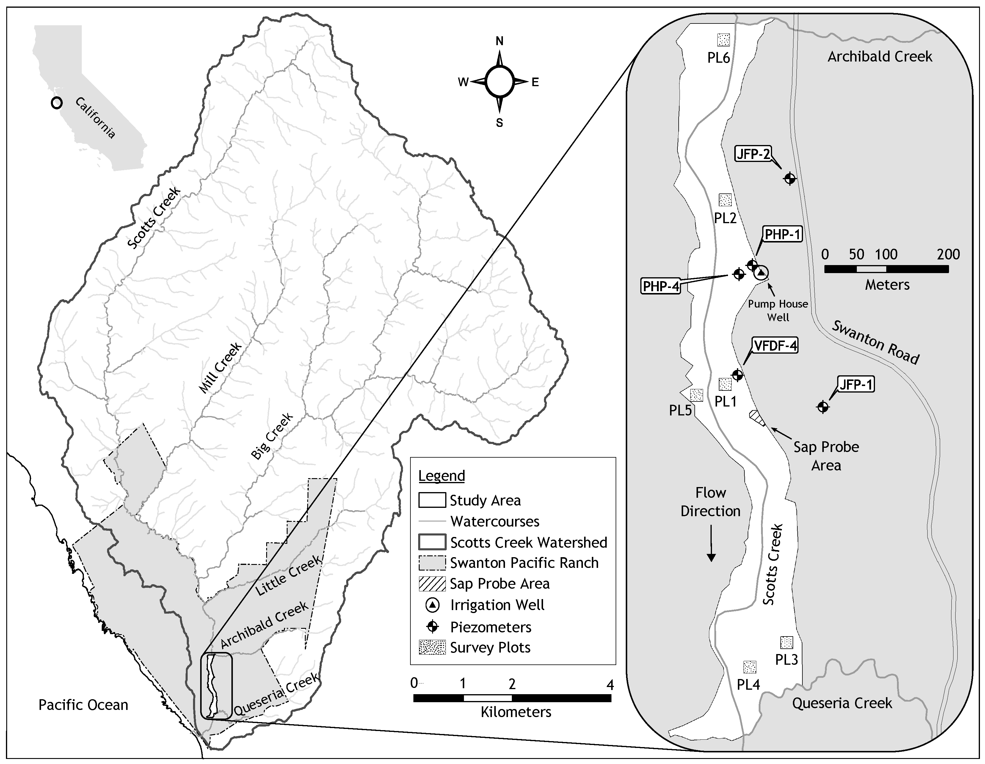
The study was conducted at Swanton Pacific Ranch, located along the Pacific coast in Santa Cruz County, California, about 84 km south-southeast of San Francisco. A map of the watershed and study area is shown in Figure 1. The climate of the region is Mediterranean, with warm, mostly dry summers and cool, wet winters. The mean summer air temperature highs are 24 C and mean winter air temperature lows are 5 C. The rainy season is typically from October to April, with an average yearly precipitation of 975 mm, with an average of 193 mm occurring in January. Even during the recent prolonged drought in California from December 2011 to March 2019, the average yearly precipitation was 945 mm. The average yearly precipitation over the duration of this study (August 2017 through August 2019) was 855 mm. Streamflow in main stream in the watershed, Scotts Creek, is typically very low in the summer (≤0.1 m/s). During the winter, peak flows typically are 20–70 m/s, based on data from a Scotts Creek stream gauge.
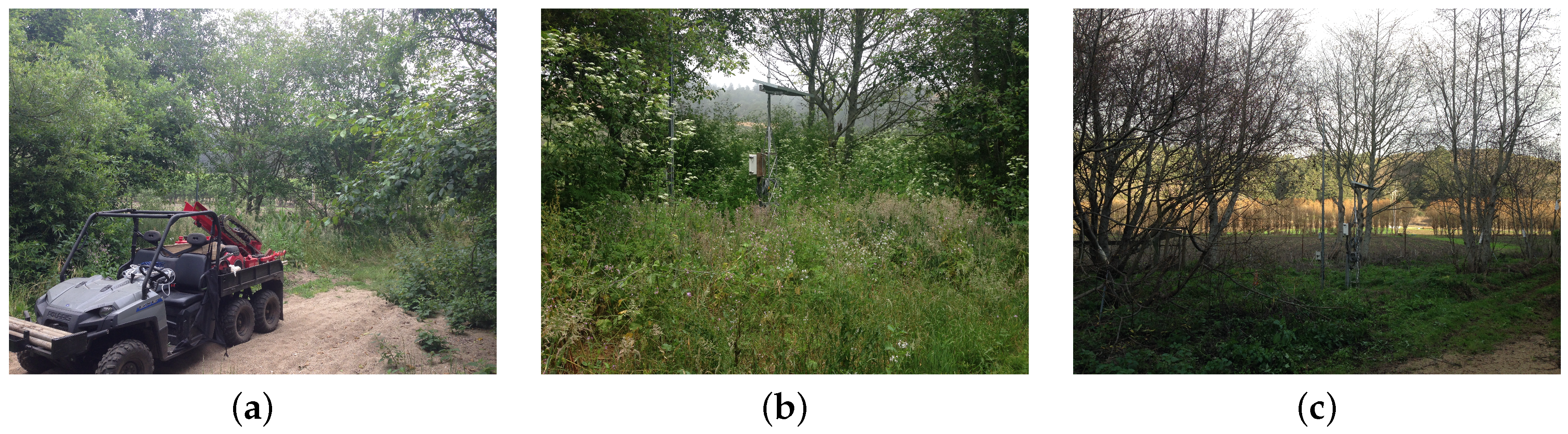
The riparian corridor within the study area is about 70–140 m wide with a canopy cover that often approaches 100% during the growing season [21]. The dominant trees along the lower portion of the Scotts Creek watershed are red alders (Alnus rubra Bong.), arroyo willows (Salix lasiolepis Benth.), and pacific willows (Salix lasiandra Benth. var. lasiandra). Other trees include box elder (Acer negundo L.), bigleaf maple (Acer macrophyllum Pursh.), California bay laurel (Umbellularia californica (Hook. & Arn.) Nutt.), and coastal redwoods (Sequoia sempervirens (D. Don) Endl.) Common understory vegetation includes California blackberry (Rubus ursinus Cham. & Schltdl.), stinging nettle (Urtica dioica subsp. gracilis L.), poison hemlock (Conium maculatum L.), Cape ivy (Delairea odorata Lem.), and Italian thistle (Carduus pycnocephalus L. subsp. pycnocephalus) [21,22,23]. The phreatophytes documented within the study area, including red alders, arroyo willows, pacific willows, box elders, and bigleaf maples, are all deciduous. They typically lose their leaves in November/December and their leaf buds burst in early March. They maintain maximum leafage for most of the spring, summer, and fall growing seasons. The typical site vegetation is shown in Figure 2, which shows (a) the dominant phreatophytic trees (b) understory vegetation, and (c) deciduous vegetation during winter dormancy. Red alders are fast-growing, relatively short-lived, shade intolerant, and tend to favor sites with bare mineral soil and high sun exposure that were disturbed by floods, windthrows, logging, or fires.
2.2. Sap Flow Measurements
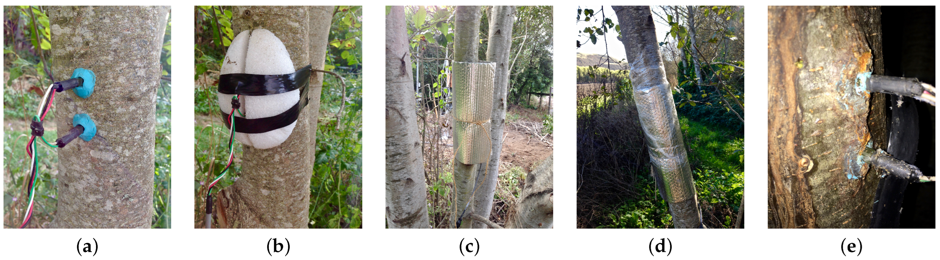
Four trees of the dominant phreatophytes at the study site were selected for monitoring based on their stem diameters (7.6–12.7 cm) and proximity (less than 33 m) to the data acquisition station. The location of the sap flow probe area is shown on the site map in Figure 1. A pair of probes was installed in each tree. The installation procedure involved removal of the outer bark at 1.22–1.45 m above the ground to minimize radiative temperature effects from land surface. Two pilot holes, 40 mm apart vertically, were then bored into the tree stem to a depth of 30 mm using a 1.5-mm diameter drill bit. The pilot holes and drill bit were flushed with 10% chlorine bleach prior to and after boring the holes in each tree to minimize the introduction and spread of pathogens. The probes were then carefully inserted into the bores and adhesive putty applied around the base of each probe to provide a water-tight seal. Foam covers were placed over the probes for thermal insulation and to protect the electrical wiring. Reflective bubble insulation was wrapped around the probes, foam, and tree stem to minimize thermal gradients caused by direct solar radiation. Saran wrap was wrapped around the tree stem and upper portion of the reflective bubble insulation to prevent water from flowing down the stem surface and into the probes. Figure 3 depicts the probe installation steps (a)–(d) and the aftermath of tree healing that occurred over the study period (e).
The probes were part of the FLGS-TDP XM1000 sap velocity system (Dynamax Inc., Huston, TX, USA), which includes a CR1000 measurement and control data logger with a AM16/32 relay multiplexer (Campbell Scientific, Logan, UT, USA) housed in a rugged weather-resistant instrument enclosure. Communication, programming, and data extraction between the data logger and a computer were facilitated using the PC400 data logger support software (Campbell Scientific). The data logger and solar panel were mounted on a 10-ft UT10 aluminum tower in a forest canopy gap. The tower was secured in an 8-ft concrete pad with a J-bolt kit for stability during rough weather and flooding. Probe cords were placed inside 1.0-inch diameter schedule 40 PVC conduit pipes and installed approximately 30 cm underground for protection against weather, flooding, and wildlife. The conduit pipe openings were covered with duct seal putty to keep out moisture. Upon completion of probe installation and mounting the data logger to the tower, sap temperature differentials were recorded at one-minute intervals and their averages were recorded every 15 min. The data were downloaded from the data logger every two months. A sap flow computation spreadsheet, provided by Dynamax Inc., and modified appropriately to implement the theoretical equations of [14], was used to calculate the volumetric rate of sap flow.
2.3. Measurement and Estimation of Tree Diameter and Sapwood Depth
Determination of the sapwood area, , requires knowledge of tree stem diameters, d, and sapwood depth, . Hence, for this work, tree stem diameter, d, at breast height (herein ) was measured for all woody vegetation greater than 0.025 m in diameter in each of the six representative sample plots. For this work, the breast height used was 1.37 m. The stem diameters were measured manually with a standard English diameter tape. The tree diameter tape is based on the assumption that tree stems are perfect circles such that , where C is tree stem circumference. Within each plot, the number of species, and number of trees for each species were also recorded.
Whereas tree stem diameter was measured for all woody vegetation in each of the sample plots, sapwood depths, , were measured from cores extracted from a small representative subset of the riparian phreatophytic trees within each plot. A stratified random sampling design was used to estimate phreatophytic vegetation composition. Woody vegetation was sampled in six random plots, each of area 400 m, within the riparian corridor. Environmental Systems Research Institute’s (ESRI) ArcMap 10.7 was used to determine the locations of these random plots. First, a fishnet with 20 m × 20 m sections was laid over the study area in ArcMap. Then, random sections were chosen on the grid. The coordinates of the northwest corner of each plot were programmed into a Trimble Geo 7X handheld GPS for locating in the field. The locations of the remaining three corners for each plot were determined with an open reel measuring tape and a compass.
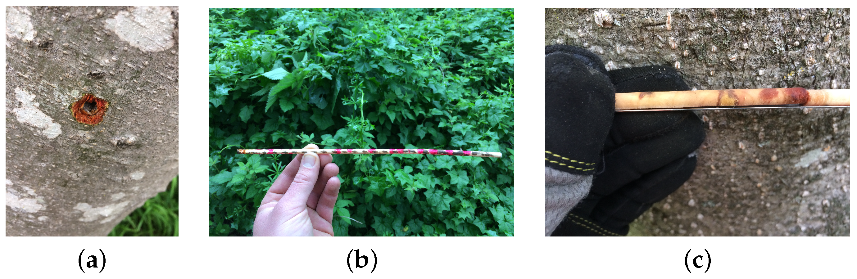
To measure , wood cores were extracted at breast height (1.37 m) from select phreatophytes using an increment borer (Haglöf Sweden AB) within each plot. The bark thickness, sapwood depth, and heartwood/pith radius of each core were measured in the field with a ruler. In most trees, the sapwood’s lighter color made it simple to distinguish from the heartwood. However, in some trees (e.g., red alders and arroyo willows), there was very little color difference between the sapwood and heartwood [24]. In order to determine the sapwood depth, , wood cores were first stained with a 0.2% safranin dye by applying the dye to each core in a series of continuous drops using a small pipette. The dye was applied immediately after extracting the cores because the vessels of vascular system lose uptake pressure [25]. Because the dye is absorbed more easily by sapwood than by heartwood [26], it allows one to locate the sapwood and heartwood boundaries from which could then be estimated. Figure 4 depicts (a) the bore from which a core sample was retrieved, (b) an example of a retrieved tree core stained with dye, and (c) a close-up of the core showing sap wood to heartwood transition.
The sapwood depth, , of phreatophytic trees in each plot was measured in only a subset of the trees on the plot. Here, we outline the approach used to estimate , and the sapwood areas, , of the non-sampled trees. Sapwood depth is defined as
where d is tree diameter at breast height (DBH), is bark thickness, and heartwood/pith radius. Estimates of bark thickness for non-cored trees of known diameter, d, were estimated using the relation of [27], namely
where and are empirical parameters determined using data from cored trees. Estimates of heartwood/pith radii were obtained using the relation
for red alders, and
for willows, where and are empirical parameters determined using data from cored trees. For cored trees, the measured bark thicknesses and heartwood/pith radii were plotted against the measured stem diameters and best fits of the models given in above were obtained to determine the values of the empirical parameters. With the empirical constants thus determined, Equations (2)–(4) were then used to estimate values of and for the non-cored trees given their measured diameter d.
For cored samples, the dye droplet method was used to determine the boundary between sapwood and heartwood. The dye was applied to every core immediately after extraction from the tree but yielded mixed results depending on the quality of the wood cores and the tree. On some cores, especially those from small trees, the sapwood absorbed the dye immediately. Heartwood in cores from older trees absorbed the dye at very slow rates, making it challenging to make the distinction between heartwood and sapwood in a timely manner. There were multiple instances where sapwood and heartwood could not be distinguished from each other based on dye absorption. In these cases, changes in color and/or texture were used to determine the sapwood/heartwood boundary. Overall, determining the boundary between sapwood and heartwood was very difficult, even with the dye droplet method.
2.4. Upscaling Plot Measurements to Forest Scale
Sapwood area is a measure of the actual tree stem area through which water extracted from the subsurface flows on its way to be transpired to the atmosphere from the canopy. The sapwood areas of all phreatophytic trees in six sample plots of the riparian forest were used to estimate the fractional sapwood basal area, (expressed in /ha), for each phreatophytic species over the riparian forest within the study area using the following relation adapted from [28]:
where M is the number of sample plots, is the number of trees of species in the sample plot, is the forest floor area of the sample plot, and is the sapwood area of the tree of the species in the plot. In this work, the area of each of the six () sample plots in which trees were counted and core samples collected, was fixed at . The total sapwood area, , of a given phreatophytic species over the entire riparian forest within the study area was then estimated as simply
where is the measured total ground area of the forest. For this study, ha.
The total riparian forest sapwood area determined with this equation was then with sap flow data from the four instrumented trees to upscale measured sap flow to the riparian forest ET. First, the ET from each instrumented tree was calculated based on the areal extent of its canopy [29]. The canopy extent of each instrumented tree was determined with a Trimble Geo 7x GNSS handheld. In ArcMap, the GPS points of each tree were connected to create a polygon that represented the areal extent of the canopy. A modified version of an equation from [16] was used to calculate ET above the riparian corridor canopy viz.,
where N is the number of tree species, is the mean sap flux density of the phreatophytic species and is the combined canopy areal extent of the riparian forest. For simplicity, arroyo and pacific willows are treated as one species for this study such that the number of species was (red alders and willows). This was necessitated by the fact that only one willow was instrumented.
2.5. Validation Method
The upscaled results will be validated by comparison to two common methods to estimate ET, namely the Modified Penman Equation for computing reference evapotranspiration () and an equation utilizing normalized difference vegetation index (NDVI) data and meteorological data. The original Penman Equation comprises two terms: energy (radiation) and aerodynamic (wind and humidity) [30]. The Modified Penman Equation includes an amended wind function [31]. According to [32], the Modified Penman Equation has been shown to overestimate in conditions with high winds and low evaporation, but it offers the best estimates for grass surfaces. The (mm/d) was calculated using
where c [-] is an adjustment factor compensating for difference in day and night weather conditions, W [-] is a temperature related weighting factor, (mm/d) is the net solar radiation in equivalent ET, [-] is a wind-related function, and VPD (mbar) is the vapor pressure deficit.
The second method for estimating ET is via satellite remote sensing and meteorological data. Remote sensing provides spatial and temporal coverage of the land surface [33]. NDVI is one of the many products that comes from remote sensing and it quantifies the density of green vegetation on a plot of land. Comprising imagery with near-infrared and red spectral bands, NDVI data are useful for monitoring changes in vegetation [34]. Due to chlorophyll in the leaves, vegetated areas absorb visible light and have high near-infrared reflectance. In contrast, non-vegetated features have high visible light reflectance and low near-infrared reflectance, namely rocks, bare soil, water, snow, and clouds. Using an equation by [35], the ET of the riparian forest can be calculated with
where (W/m) is the net solar radiation, [-] is the aerodynamic and canopy resistance parameter, is the slope of the saturated vapor pressure curve, (kg/m) is the density of water, (J/kg) is the latent heat of vaporization of water, and (kPa/K) is a psychrometric constant. The parameter was estimated from a scatter plot of site surface temperature and NDVI data using the linear interpolation scheme described in [35], where .
The data set consisted of hourly ET data reported by a California Irrigation Management Information System (CIMIS) automated weather station located 21 km from the study area, in Santa Cruz. The station uses the CIMIS version of the modified Penman-Monteith Equation [30] given by [31] to calculate ET from a standardized grass surface that is well-irrigated and closely cut, while completely shading the soil. NDVI and meteorological data were used to calculate the ET of the riparian forest with Equation (9). The NDVI data were taken from weekly EROS Moderate Resolution Imaging Spectroradiometer (eMODIS) composite sets at spatial resolution [36]. The weighted average NDVI value of the entire study area each week was calculated in ArcMap by determining the percentage of study area within each pixel. The NDVI values were calculated using , where IR and R represents pixel values from the infrared and red bands, respectively. This yielded NDVI values in the range −1 to +1 for use in Equation (9). Required meteorological data comprised air pressure, air temperature, and solar radiation. Two sets of these data were taken from two separate weather stations (CIMIS and Weather Underground) within the general vicinity of the study area in order to compare sap flow based-ET to separate areas with slightly different weather patterns. The second station was a nearby Weather Underground (WU) station, located 5 km from the study area in Davenport, CA. The meteorological data of each weather station were averaged over the same weeks as the eMODIS composite sets.
3. Results
As stated previously, the objective of the work was to estimate riparian forest ET from sap flow measurements collected in a small sample of the predominant vegetation. The ET estimates are based on estimates of the total sapwood area for the entire riparian forest as well as its canopy areal extent. The results are presented in the following.
3.1. Phreatophytic Vegetation Survey and Sapwood Area
A total of 159 trees were surveyed in the six sample plots, with 153 of them being phreatophytes. They comprised 83 red alders, 61 arroyo willows, 9 pacific willows, and 6 coastal redwoods. The survey comprised direct measurement of DBH using diameter tape. Sapwood depth was measured directly in a subset of the surveyed phreatophytes by wood coring. The coastal redwoods are not considered phreatophytes, and thus were excluded from the calculations for the total sapwood area of the riparian forest. The survey results, including averages and standard deviations of DBH and sapwood area, are summarized in Table 1. The values in parentheses are for the subsamples that were selected for coring to obtain direct measurements of bark thickness and heartwood/pith radius for sapwood area estimation. Multiple cores were extracted on some trees because the heartwood and/or piths were difficult to sample. Larger trees were especially difficult to sample due to irregularities in radial growth of tree stems. The poor surface quality of the cores and the small difference in color between early wood and late wood made determining the age of trees challenging. Wood cores from young, small red alders (DBH of cm) consistently showed only bark, sapwood, and piths, which agree with [17].
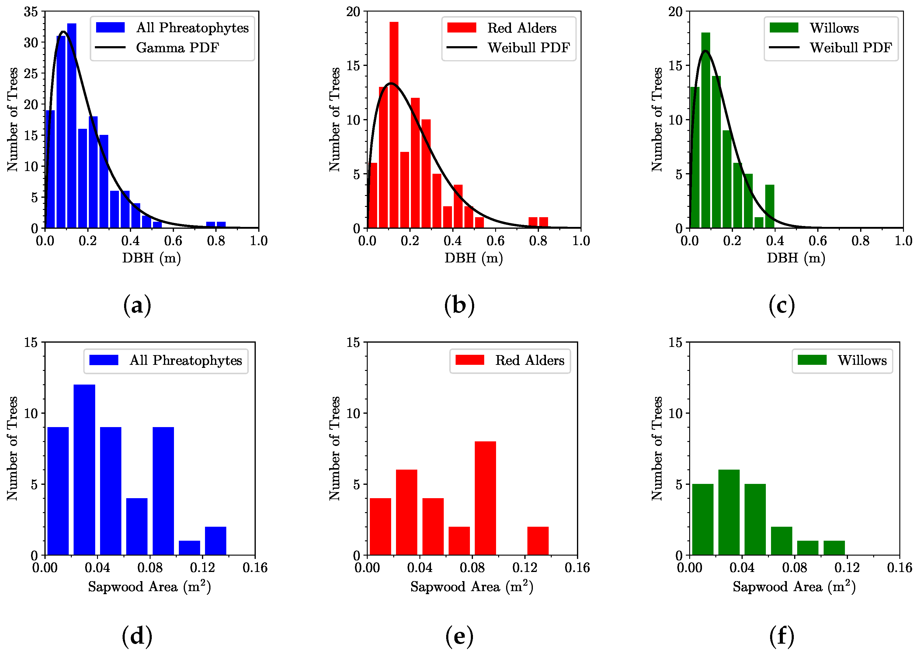
The histograms of the measured diameters at breast height for all surveyed phreatophytes are shown in Figure 5. Theoretical probability density functions are also included for completeness. The arroyo willows and pacific willows were analyzed as one composite group due to their small sample sizes (61 and 9, respectively). Weibull ( for willows and for red alders) and lognormal ( for willows and for red alders) distribution model fits are also included. When the red alders and willows were analyzed as one composite phreatophytic vegetation group, they appear to follow gamma () and Weibull () distributions based on a 95% confidence interval. All the probability density functions show positive skewness indicating a sampling bias on the small tree diameter end of the range. Figure 5 also shows histograms of cored main stem sapwood areas for red alders, arroyo willows, and pacific willows from the six sample plots.
Estimates of model parameters in Equations (2)–(4) from tree core data are summarized in Table 2. These parameters were used to estimate sapwood basal area for the trees on which cores were not obtained but for which the diameter d at breast height was measured. Estimates of the fractional sapwood basal area and sapwood area across the entire riparian forest using Equations (5) and (6), respectively, are also summarized in Table 2.
3.2. Sap Flow Measurements
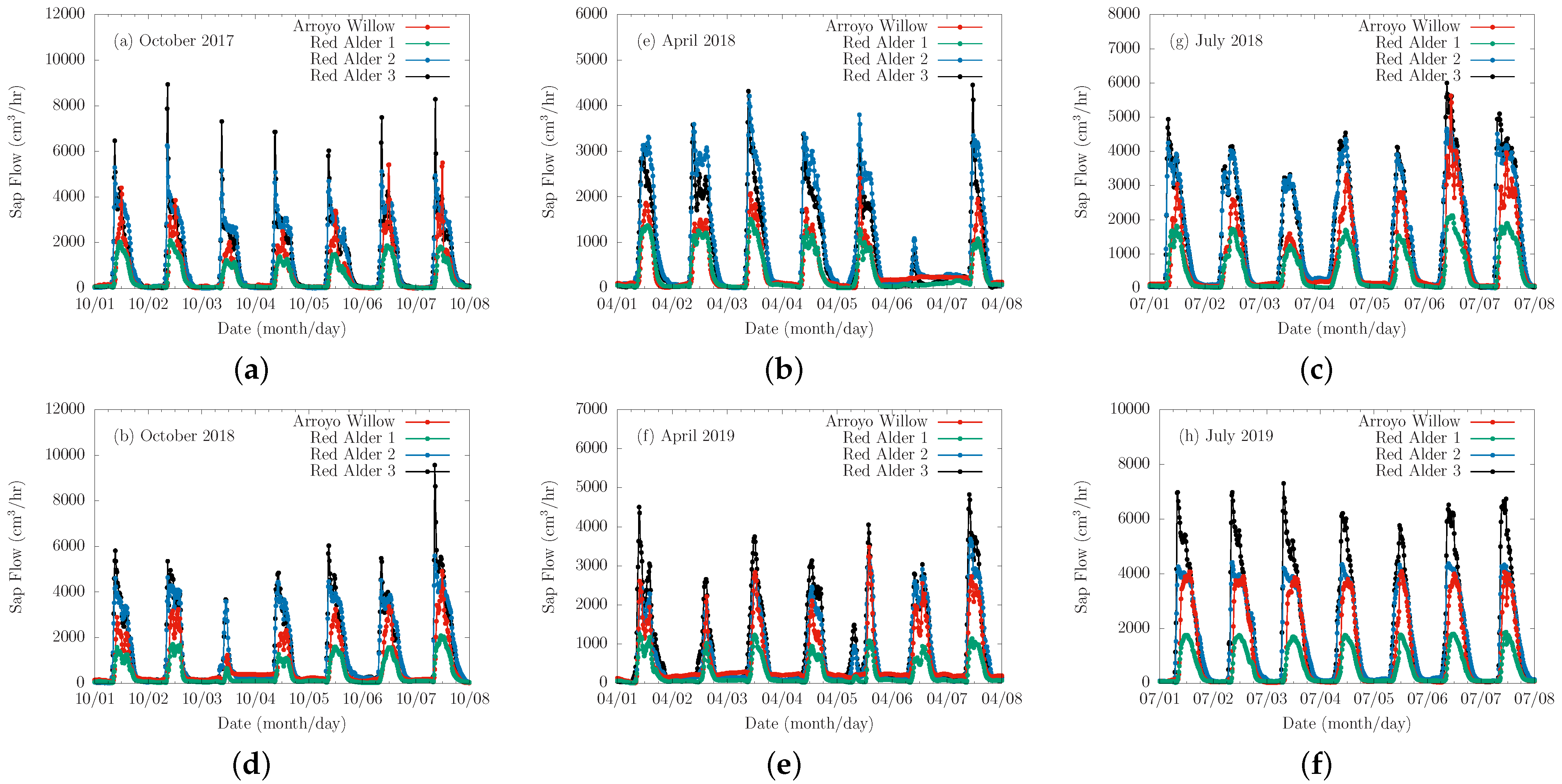
The four instrumented trees were continuously monitored at one-minute intervals and the data averaged every 15 min for 618 consecutive days from 18 August 2017 through 26 April 2019. The diurnal sap flow data for selected weekly periods in the growing seasons of each study year are shown in Figure 6. Several instances of morning peaks were observed in the data. They were particularly evident during the growing seasons of the study period for red alders 2 and 3 (Figure 6a), and attributable to direct incident solar radiation on the reflective shield wrapped around the probes, which served to minimize the occurrence of morning peaks. It may also indicate problems with installation of the probes. Another possibility is that they may be as a result of water release in the morning from tree trunk storage before tree roots uptake water to refill the storage according to [37,38] who found that tree trunk internal water storage can contribute as much as 28% of the daily water budget in some tree species. The arroyo willow and red alder 1 also show morning peaks, but had much lower amplitudes later in the morning. The time lag time between sunrise and initial sap flow for the arroyo willow and red alder may be due to partial shading by other trees. All instrumented trees showed some activity during the winter period of dormancy, with the peak amplitudes of greater than an order of magnitude smaller than those observed during periods of active growth.
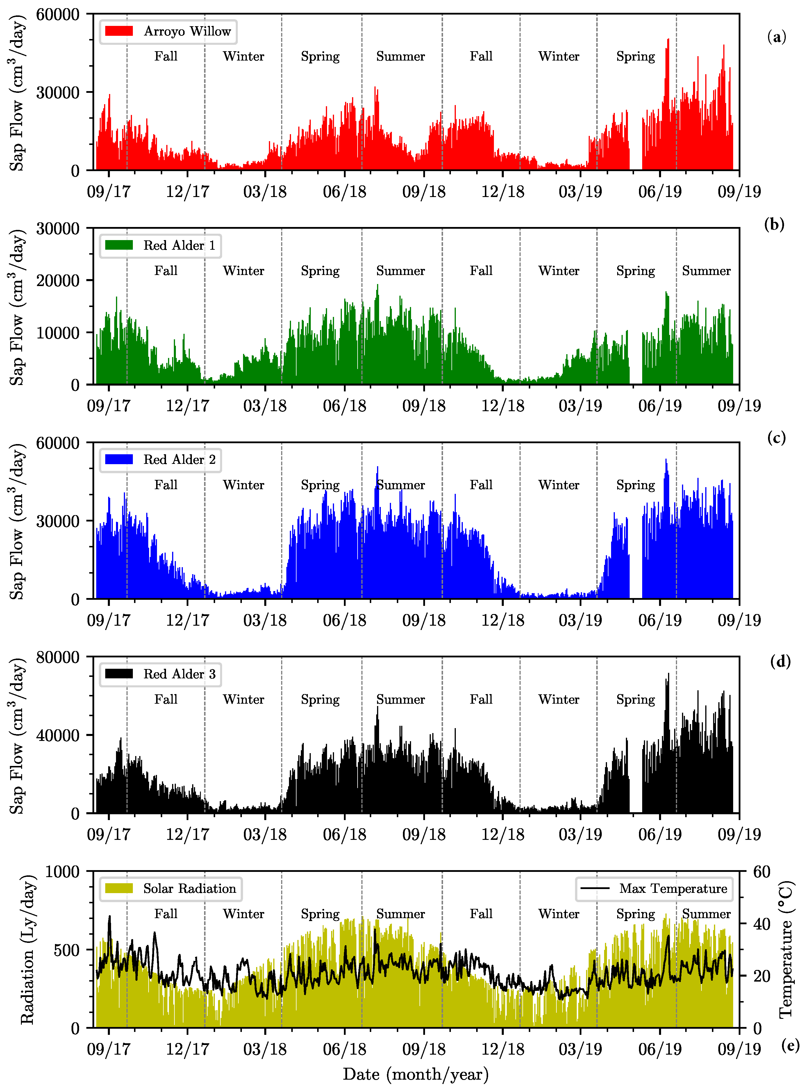
The time series of the sap flow data for the entire two-year monitoring period of the four instrumented trees are shown in Figure 7 for (a) arroyo willow, (b) red alder 1, (c) red alder 2, and (d) red alder 3. The daily maximum air temperatures and daily mean solar radiation over the same monitoring period are included in Figure 7e to highlight the seasonality of the observed behavior. Seasonality is clearly evident in the sap flow data with periods of high sap flow generally coinciding with spring, summer and fall seasons, interspersed with periods of minimal flow in winter seasons. The spring-fall period is the period of active growth, with leafage increasing to summer-fall maxima. The instrumented phreatophytes were deciduous, losing leaves in late fall, with complete leaf loss deep in the winter months of dormancy. Fall, winter, spring, and summer seasons are marked clearly on the figures to highlight their correlation to periods of significant sap flow change. Specifically, the active and dormancy periods of all four trees clearly follow the spring equinoxes and winter solstices (Figure 7).
Sap flow peaked in the arroyo willow in early July 2018 and early June 2019. It was dormant from early January 2018 to early March 2018, and mid-December 2018 to mid-March 2019. It also showed a similar sap flow pattern to red alder 1 by mid-December 2018. Its sap flow pattern returned to normal by mid-March 2019. Mean peak sap flow in red alders occurred in early July 2018 and early June 2019. In general, the red alders were dormant from December to mid-March. Red alder 1 was dormant from early November 2017 to mid-March 2018 and mid-November 2018 to mid-March 2019. Red alder 2 was dormant from December 2017 to late March 2018, and late November 2018 to late March 2019. Red alder 3 was dormant from late December 2017 to late March 2018 and from mid-December 2018 to mid-March 2019. These results generally agree with those of [17], whose red alders were dormant during the winter period, though the period of dormancy is appreciably longer in Oregon, extending from October through March.
3.3. Evapotranspiration of Riparian Forest
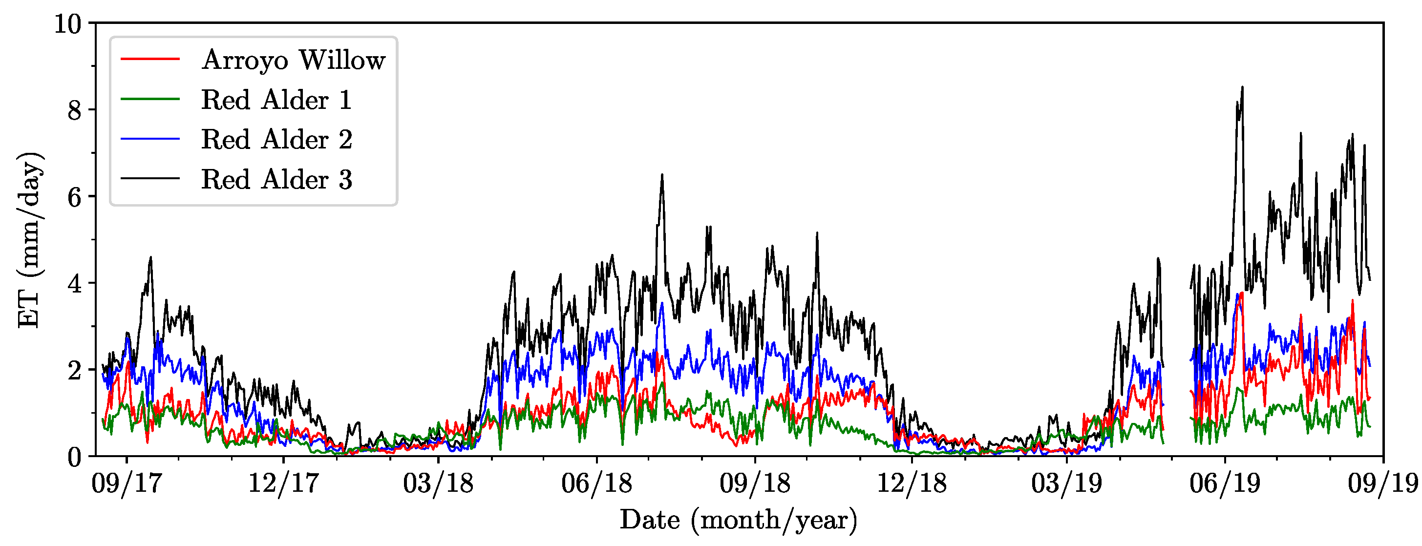
Sap flow data were first used to estimate the ET of the individual instrumented trees. The results are shown in Figure 8. The seasonal variation in ET of the individual trees is clearly evident as one would expect from the sap flow data shown in Figure 7. The ET data among the four trees appear to show moderate to strong behavioral correlations, with red alders 2 and 3 consistently showing greater ET than the other two trees during the peak flow periods. The results obtained here did not show a general decrease in ET over the period of the study as has been observed by other workers. In fact, two trees (arroyo willow and red alder 3) appear to show increased ET in the final year (2019) of the study. The seasonal averages of the computed ET for the four trees are summarized in Table 3.
The sap flow data collected from the four instrumented trees were upscaled to the entire riparian forest canopy using Equation (7), and the estimated values are summarized and included in Table 3. The season averaged values range from a low of 0.5 mm/d during the winters to a high of 4.1 mm/d over the summer. Daily values show peak values in excess of 6 mm/d. It should also be noted that the winter average values are within margins of instrument measurement uncertainty.
The ET of the riparian forest estimated from sap flow data was compared to ET estimates based on NDVI and meteorological data, and in the general vicinity of the study area. The seasonal averages of the sap flow-based ET, , and are summarized in Table 4. Generally, there is strong correlation in the observed temporal behavior, as well as moderate agreement in estimates of ET over the active growing periods of spring, summer, and fall. This is particularly the case when comparing the sap flow-based ET to . However, there are notable divergences in the data. In fall of 2017, the sap flow-based ET appeared to be similar to the and based on CIMIS and WU data (Figure 9a). In winter of 2018, the sap flow-based ET was substantially lower than the and both estimates. In spring of 2018, the sap flow-based ET was marginally lower than the , but was substantially lower than both values. In summer of 2018, sap flow-based ET was similar to , but it was marginally lower than the and . This pattern was repeated in the second year of the study period.
The residuals of the ET, defined as the differences between the sap flow-based ET and the other methods, are shown in Figure 9b. The dashed red and blue lines on the graph in the figure mark and mm/d residual bounds, respectively. The residuals are highest during winter and early spring, during which periods the exceed 2.0 mm/d. The ET predicted by the other methods largely exceeds that based on sap flow due to dormancy of the willows and red alders during the winter seasons. During the mid-summer to late fall periods, the residuals are mostly within mm/d, indicating relatively strong agreement between sap flow-based ET and the other methods.
Scatter plots of sap flow based ET estimates versus the other three methods mentioned above are shown in Figure 10. The data show positive correlations between sap flow-based ET estimates and and the NDVI based estimates, with high variance and some bias as much of the data scatter is widely distributed above the 1:1 line (dashed red line). Data points above the 1:1 line indicate that sap flow-based ET was lower than the and the NDVI based ET. Table 5 shows the slopes and coefficients of determination () of the scatter plots with and without the winter data. Excluding winter data marginally improved the slopes and values. The fact that the slopes of the regression lines are higher than 1:1 is an indication of overall bias in the sap flow-based ET prediction of the and NDVI/weather-based ET. The excluded winter data are marked in cyan in Figure 10b, where the data clearly plot above the 1:1 line, which confirms the observation made above that sap flow-based ET underestimates winter ET predicted by the other methods.
3.4. Comparison with Groundwater Pumping for Irrigation
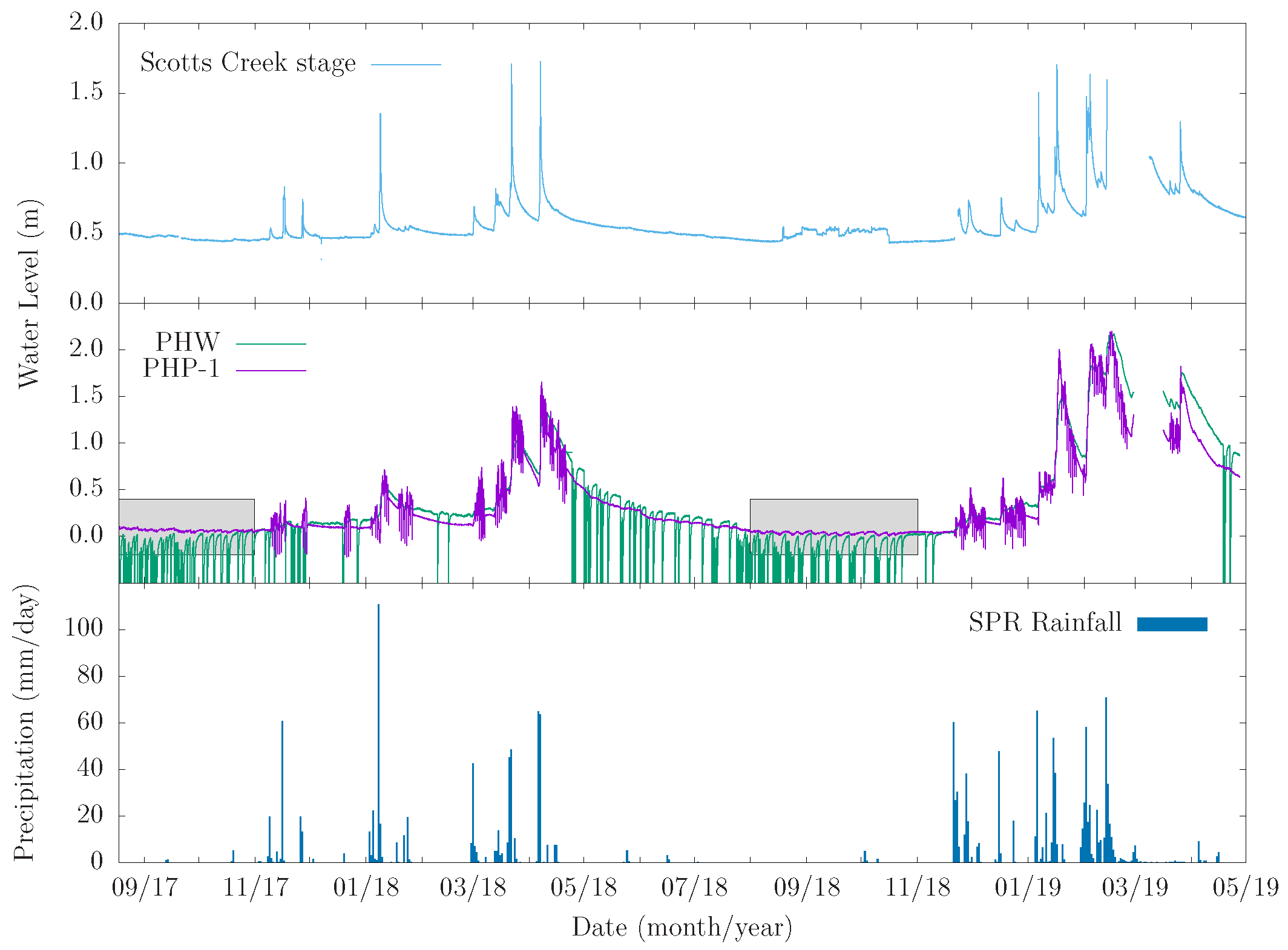
Groundwater fluctuations were continuously measured in five piezometers (JFP-1, JFP-2, PHP-1, PHP-4, and VFDP-4 in Figure 1) and the Pump House irrigation well from 18 August 2017 to 27 April 2019. All piezometers are completed in a thin clay/silt aquitard layer that sits atop the underlying leaky confined aquifer [39], and all responded to riparian forest ET as well as to pumping from the Pump House irrigation well. Data from the irrigation well and the most responsive of the piezometers, PHP-1, are shown in Figure 11 and Figure 12 and are also reported in [20]. Piezometer and well data are reported here as changes relative to the respective first water level recorded to facilitate their comparison. Piezometer PHP-1 and the Pump House irrigation well are about 18 m apart. The data show fluctuations that are clearly caused by groundwater pumping, ET, recharge primarily from winter-spring precipitation events, and long-term discharge to the stream and ocean characterized by a period of recession from the end of spring through the summer and into the fall.
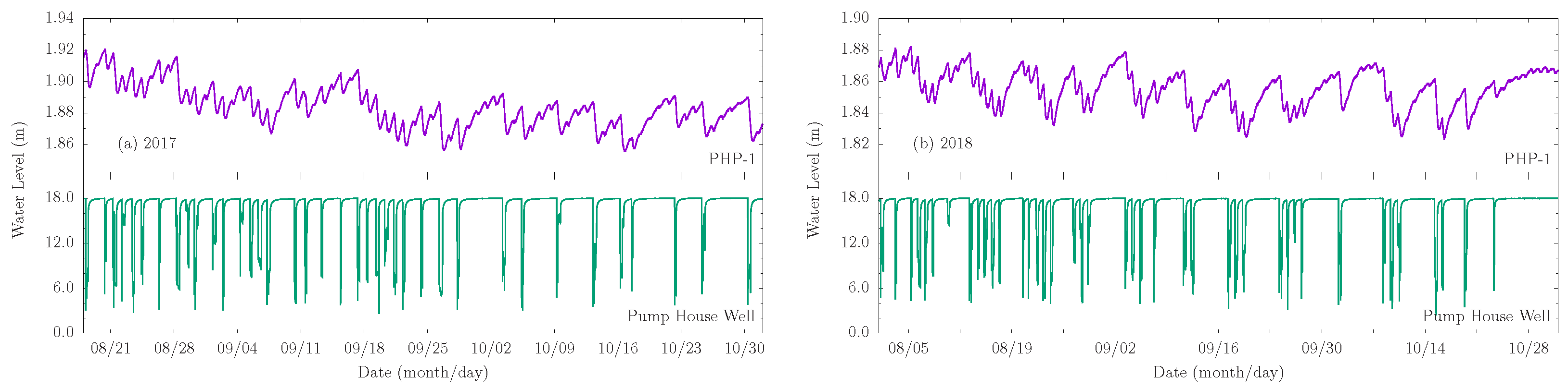
Diurnal groundwater level fluctuations due to ET forcing are superposed on those due to pumping from the irrigation well. Fluctuations due to ET are more pronounced in the piezometer data and are largely imperceptible in the irrigation well data. They are highlighted in Figure 12, which shows zoomed in plots of the aquifer and aquitard responses for two monitoring periods (08/2017–11/2017 and 08/2018–11/2018). Groundwater response to ET is most perceptible during periods of aquifer and aquitard recovery following a pumping event from the irrigation well. When the pumping frequency is daily, water-level responses to ET are practically indistinguishable from those attributable to pumping. In such cases, the amplitude of the aquitard response is much larger than what can be expected from ET alone. The data clearly show that the riparian corridor phreatophytes induce measurable fluctuations in the thin clay/silt aquitard that overlies the leaky aquifer.
The diurnal groundwater fluctuations due to ET discussed above are induced by a forest-scale ET flux averaging 3.8 mm/d over the summer seasons. When multiplied by forest area, ha, this flux yields a volume flow rate usage by phreatophytes of gpm. The typical pumping rate from the irrigation at the site is 250 gpm. Hence, ET across the forest amounts to about 25% the pumping rate, which is a substantial proportion.
4. Discussion
As stated previously, the objective of this work was to estimate riparian forest ET from sap flow measurements collected in a small sample of phreatophytic trees. Sap flow measurements were collected in the same four trees over the two-year monitoring period. For each individual tree, the data were largely repeatable during the growing seasons, with comparable average seasonal amplitudes. The fact that sap flow probes were left in the trees for such a prolonged period but continued to yield meaningful measurements was unexpected because [40] reported that other users of the sap flow probes used the same drill holes for one growing season, at the most. In addition, ref. [18] reported a 30% decrease in daily average sap flux density during the second growing season for red alders. The degradation of data quality over prolonged periods of monitoring has been attributed to tree response to drill-hole wounding by forming tyloses over those vessels, which affects heat exchange with the probes [41]. The good quality data collected over two-year study period may be attributable to the fact that the four instrumented trees were younger, smaller, and of different species than those in other studies. Hence, it may be argued that younger trees are better suited for prolonged monitoring than are older trees as long as their diameters and sapwood areas are corrected for from year to year in the computation of ET.
The ET flux projected across the entire riparian forest correlated strongly with the CIMIS and ET computed on the basis of NDVI/meteorological data. The sap flow-based forest ET had consistently lower average magnitudes during the growing seasons with significant departure from the values computed by the other methods over the winter seasons. This divergence in winter may be due to vegetation differences among the methods. Sap flow-based ET was collected on deciduous trees that lost their leaves every winter leading to values that were consistently lower than those from the other methods. The CIMIS values are based on a cool-season perennial grass that does not die back during winter and continues to transpire. Additionally, although most trees lost their leaves along lower Scotts Creek in winter, there was still plenty of green understory vegetation and some evergreen overstory vegetation, which were shown by the NDVI data. This may explain why the ET residuals showed seasonal patterns with peaks being highest and smallest during winter and fall seasons, respectively.
Long-term passive groundwater monitoring data were analyzed qualitatively to assess the magnitude of fluctuations in water levels from season to season and year to year. On average, at the study site, groundwater levels increased every winter before receding and reaching their lowest levels in the fall. The steady decrease in water levels during the summer and fall is largely attributable to ocean and stream discharge, consumption by phreatophytic vegetation [42], and groundwater withdrawal for crop irrigation. Diurnal groundwater fluctuations attributable to uptake by phreatophytes across the study forest are much smaller than fluctuations due to pumping, with sap flow based estimates of ET over the riparian corridor being about 25% the typical pumping rate for irrigation. Sap flow based estimates of groundwater fluctuations showed appreciable divergence from satellite based measurements, which suggests the importance of the former in calibration of the the latter, especially where site-specific vegetation may have greater control on local ET and consumptive groundwater use. A well characterized ET forcing function is essential modeling for groundwater flow and diurnal fluctuations [5,9,43,44,45].
There are some limitations in this study that may be addressed in future research, including (1) location and number of instrumented trees, (2) size of instrumented trees, (3) location and number of sap flow probes on tree stems, (4) instrumentation and monitoring of the minor tree species scattered throughout the riparian corridor such as live oak and redwoods, (5) accounting for the effect of understory vegetation on total ET and (6) measurement of sapwood area for individual trees and the entire riparian forest. The sampling design for this study was partly restricted due to the stem-diameter limitation of the probes, which biased monitoring to younger trees that are known to be hydraulically active than older trees. Using a combination of small and large sap flow probes to see the differences in sap flux density could provide more accurate estimates of ET. Additional pairs of probes could be installed on each instrumented tree at different depths and the sap flux densities averaged because the sap flux density is not uniform across sapwood area of a tree [15,16]. The method of using long-term sap flow measurements to estimate the ET of a riparian forest may be replicated on other phreatophytic species for similar or longer periods of time because phreatophytic tree species may react differently to sap flow probes in terms of sap flow behavior and physical intrusion of the probes.
5. Conclusions
The study presented herein was based on a two-year sapflow monitoring program on a single riparian forest plot where only a small sample of four trees were instrumented. The data were used together with a survey of tree sapwood depth in six plots across the entire forest to upscale the single-plot sapflow measurements to forest canopy-scale evapotranspiration (ET). The upscaled ET results were compared to ET based on NDVI-based estimates and were shown to be in good agreement. This indicates that for expensive ground-based technologies such as sapflow sensing by the heat dissipation models, a instrumentation of a small sample of a forest may yield reasonable estimates of forest canopy-scale ET as long as they are also based on sampling of sapwood depth across the entire forest. The results of the present study, despite the small sample size of sap flow measurements, illustrate the importance of ground-based measurements of sap flow for calibrating satellite based methods and for providing site-specific estimates and to better characterize the ET forcing in groundwater flow models. The small sample size is important because it is necessitated by the high cost of instrumenting individual trees and it suggests the potential usefulness of single-plot monitoring stations for ground-based measurement and estimation of forest ET.
Further research is required to better capture the spatial variability of sapflow across the forest and would include: (1) a larger sample of instrumented trees to better characterize sap flow behavior, (2) a sample of instrumented trees with a greater variety of main stem diameters in order to better characterize the sap flux density for each species, (3) greater spatial distances between instrumented trees, and (4) long-term monitoring of sap flow in additional phreatophytic species across the forest. The need for a greater sample size is clear even from the data from four instrumented trees because they very had different canopy and sapwood areas. Tree with larger sapwood area tend to have higher volumetric sap flow rate, which could bias the results based on a small sample size.
Author Contributions
Conceptualization, B.M. and J.S.; methodology, J.S.; software, J.S.; validation, B.M. and J.S.; formal analysis, B.M. and J.S.; investigation, B.M. and J.S.; resources, B.M.; data curation, J.S.; writing—original draft preparation, B.M.; writing—review and editing, B.M. and J.S.; visualization, J.S.; supervision, B.M.; project administration, B.M.; funding acquisition, B.M. All authors have read and agreed to the published version of the manuscript.
Funding
This work was funded by the USDA NIFA McIntire-Stennis Program Grant No. 16-109.
Institutional Review Board Statement
Not applicable.
Informed Consent Statement
Not applicable.
Data Availability Statement
Not applicable.
Acknowledgments
This work was facilitated by Swanton Pacific Ranch (SPR) Director Brian Dietterick, Manager of Operations Steve Auten, SPR staff Grant William and Brian Cook, graduate student Devin Pritchard-Peterson, and undergraduate research assistant Aren Abrahamian.
Conflicts of Interest
The authors declare no conflict of interest.
Abbreviations
The following abbreviations and acronyms are used in this manuscript:
| CIMIS | California Irrigation Management Information System |
| DBH | Diameter at breast height |
| ESRI | Environmental Systems Research Institute |
| ET | Evapotranspiration |
| ETo | Reference evapotranspiration |
| eMODIS | EROS Moderate Resolution Imaging Spectroradiometer |
| HPV | Heat Pulse Velocity |
| NDVI | Normalized difference vegetative index |
| THB | Tissue Heat Balance |
| TDP | Thermal Dissipation Probe(s) |
| VPD | Vapor Pressure Deficit |
| WU | Weather Underground |
References
- Snider, B.; Urquhart, K.A.F.; Marston, D. The Relationship between Instream Flow and Coho Salmon and Steelhead Habitat Availability in Scott Creek, Santa Cruz County, California; Technical Report; California Department of Fish and Game, Environmental Services Division, Stream Flow and Habitat Evaluation Program: Redding, CA, USA, 1995.
- Welsch, D.J. Riparian Forest Buffers—Function and Design for Protection and Enhancement of Water Resources; U.S. Department of Agriculture, Forest Service, Northeastern Area, State & Private Forestry, Forest Resources Management: Washington, DC, USA, 1991.
- Jordan, T.E.; Correll, D.L.; Weller, D.E. Nutrient interception by a riparian forest receiving inputs from adjacent cropland. J. Environ. Qual. 1993, 22, 467–473. [Google Scholar] [CrossRef] [Green Version]
- Schultz, R.C.; Isenhart, T.M.; Colletti, J.P. Riparian buffer systems in crop and rangelands. Nat. Resour. Ecol. Manag. Conf. Pap. Posters Present. 2005, 23, 13–28. [Google Scholar]
- Gribovszki, Z.; Kalicz, P.; Szilágyi, J.; Kucsara, M. Riparian zone evapotranspiration estimation from diurnal groundwater level fluctuations. J. Hydrol. 2008, 349, 6–17. [Google Scholar] [CrossRef]
- Robinson, T.W. Phreatophytes; Water-Supply Paper 1423; U.S. Geological Survey: Washington, DC, USA, 1958.
- Naumburg, E.; Mata-Gonzalez, R.; Hunter, R.G.; Mclendon, T.; Martin, D.W. Phreatophytic vegetation and groundwater fluctuations: A review of current research and application of ecosystem response modeling with an emphasis on Great Basin vegetation. Environ. Manag. 2005, 35, 726–740. [Google Scholar] [CrossRef] [PubMed]
- Rood, S.B.; Bigelow, S.G.; Hall, A.A. Root architecture of riparian trees: River cut-banks provide natural hydraulic excavation, revealing that cottonwoods are facultative phreatophytes. Trees 2011, 25, 907–917. [Google Scholar] [CrossRef]
- Malama, B.; Johnson, B. Analytical modeling of saturated zone head response to evapotranspiration and river-stage fluctuations. J. Hydrol. 2010, 382, 1–9. [Google Scholar] [CrossRef]
- Scott, R.L.; Shuttleworth, W.J.; Goodrich, D.C.; Maddock, T., III. The water use of two dominant vegetation communities in a semiarid riparian ecosystem. Agric. For. Meteorol. 2000, 105, 241–256. [Google Scholar] [CrossRef]
- Goodrich, D.C.; Scott, R.; Qi, J.; Goff, B.; Unkrich, C.L.; Moran, M.S.; Williams, D.; Schaeffer, S.; Snyder, K.; MacNish, R.; et al. Seasonal estimates of riparian evapotranspiration using remote and in situ measurements. Agric. For. Meteorol. 2000, 105, 281–309. [Google Scholar] [CrossRef]
- Loheide, S.P., II; Butler, J.J., Jr.; Gorelick, S.M. Estimation of groundwater consumption by phreatophytes using diurnal water table fluctuations: A saturated-unsaturated flow assessment. Water Resour. Res. 2005, 41, W07030. [Google Scholar] [CrossRef]
- Johnson, B.; Malama, B.; Barrash, W.; Flores, A.N. Recognizing and modeling variable drawdown due to evapotranspiration in a semiarid riparian zone considering local differences in vegetation and distance from a river source. Water Resour. Res. 2013, 49, 1030–1039. [Google Scholar] [CrossRef] [Green Version]
- Granier, A. Une nouvelle méthode pour la mesure du flux de sève brute dans le tronc des arbres. Ann. Des Sci. For. 1985, 42, 193–200. [Google Scholar] [CrossRef]
- Granier, A.; Biron, P.; Bréda, N.; Pontailler, J.Y.; Saugier, B. Transpiration of trees and forest stands: Short and long-term monitoring using sapflow methods. Glob. Chang. Biol. 1996, 2, 265–274. [Google Scholar] [CrossRef]
- Moore, G.W.; Bond, B.J.; Jones, J.A.; Phillips, N.; Meinzer, F.C. Structural and compositional controls on transpiration in 40-and 450-year-old riparian forests in western Oregon, USA. Tree Physiol. 2004, 24, 481–491. [Google Scholar] [CrossRef] [Green Version]
- Moore, G.W.; Bond, B.J.; Jones, J.A. A comparison of annual transpiration and productivity in monoculture and mixed-species Douglas-fir and red alder stands. For. Ecol. Manag. 2011, 262, 2263–2270. [Google Scholar] [CrossRef]
- Moore, G.W.; Bond, B.J.; Jones, J.A.; Meinzer, F.C. Thermal-dissipation sap flow sensors may not yield consistent sap-flux estimates over multiple years. Trees 2010, 24, 165–174. [Google Scholar] [CrossRef]
- Bidlack, J.E.; Jansky, S.H. Stern’s Introductory Plant Biology, 12th ed.; McGraw-Hill: London, UK, 2011; p. 622. [Google Scholar]
- Malama, B.; Pritchard-Peterson, D.; Jasbinsek, J.J.; Surfleet, C. Assessing Stream-Aquifer Connectivity in a Coastal California Watershed. Water 2021, 13, 416. [Google Scholar] [CrossRef]
- Cook, B.O. Lower Scotts Creek Floodplain and Habitat Enhancement Project. Master’s Thesis, California Polytechnic State University, San Luis Obispo, CA, USA, 2016. [Google Scholar]
- Louen, J.M. Hydrologic Characteristics of Summer Stream Temperatures in Little Creek and Scotts Creek at the Swanton Pacific Ranch. Master’s Thesis, California Polytechnic State University, San Luis Obispo, CA, USA, 2016. [Google Scholar]
- West, J. Traversing Swanton Road. 2016. Available online: https://arboretum.ucsc.edu/pdfs/traversin-gswanton.pdf (accessed on 20 April 2022).
- Kutscha, N.P.; Sachs, I.B. Color Tests for Differentiating Heartwood and Sapwood in Certain Softwood Tree Species; Report 2246; U.S. Department of Agriculture, Forest Service, Forest Products Laboratory: Washington, DC, USA, 1962.
- Moore, G.W.; Aparecido, L.M.T.; Discussion of Safranin Dye injection Apparatus for Red Alders. Personal Communication, 2019.
- Bamber, R.K. Sapwood and Heartwood; Technical Publication 2; Forestry Commission of New South Wales, Wood Technology and Forest Research Division: Beecroft, NSW, Australia, 1987.
- Oishi, A.C.; Oren, R.; Stoy, P.C. Estimating components of forest evapotranspiration: A footprint approach for scaling sap flux measurements. Agric. For. Meteorol. 2008, 148, 1719–1732. [Google Scholar] [CrossRef] [Green Version]
- Avery, T.E.; Burkhart, H.E. Forest Measurements, 5th ed.; McGraw-Hill: London, UK, 2002. [Google Scholar]
- Schaeffer, S.M.; Williams, D.G.; Goodrich, D.C. Transpiration of cottonwood/willow forest estimated from sap flux. Agric. For. Meteorol. 2000, 105, 257–270. [Google Scholar] [CrossRef]
- Penman, H.L. Natural evaporation from open water, bare soil and grass. Proc. R. Soc. Lond. Ser. A Math. Phys. Sci. 1948, 193, 120–145. [Google Scholar]
- Doorenbos, J.; Pruitt, W.O. Guidelines for Predicting Crop Water Requirements; FAO Irrigation and Drainage Paper 24; Food and Agriculture Organization of the United Nations: Rome, Italy, 1977. [Google Scholar]
- Allen, R.G.; Pereira, L.S.; Raes, D.; Smith, M. Crop Evapotranspiration–Guidelines for Computing Crop Water Requirements; FAO Irrigation and Drainage Paper 56; Food and Agriculture Organization of the United Nations: Rome, Italy, 1998. [Google Scholar]
- Bisht, G.; Venturini, V.; Islam, S.; Jiang, L.E. Estimation of the net radiation using MODIS (Moderate Resolution Imaging Spectroradiometer) data for clear sky days. Remote Sens. Environ. 2005, 97, 52–67. [Google Scholar] [CrossRef]
- Lillesand, T.M.; Kiefer, R.W.; Chipman, J.W. Remote Sensing and Image Interpretation, 6th ed.; John Wiley & Sons, Inc.: Hoboken, NJ, USA, 2008; p. 756. [Google Scholar]
- Batra, N.; Islam, S.; Venturini, V.; Bisht, G.; Jiang, L.E. Estimation and comparison of evapotranspiration from MODIS and AVHRR sensors for clear sky days over the Southern Great Plains. Remote Sens. Environ. 2006, 103, 1–15. [Google Scholar] [CrossRef]
- Jenkerson, C.; Maiersperger, T.; Schmidt, G. eMODIS: A User-Friendly Data Source; Open-File Report 2010–1055; U.S. Geological Survey: Washington, DC, USA, 2010.
- Goldstein, G.; Andrade, J.L.; Meinzer, F.C.; Holbrook, N.M.; Cavelier, J.; Jackson, P.; Celis, A. Stem water storage and diurnal patterns of water use in tropical forest canopy trees. Plant Cell Environ. 1998, 21, 397–406. [Google Scholar] [CrossRef]
- Carrasco, O.L.; Bucci, S.J.; Di Francescantonio, D.; Lezcano, O.A.; Campanello, P.I.; Scholz, F.G.; Rodríguez, S.; Madanes, N.; Cristiano, P.M.; Hao, G.Y.; et al. Water storage dynamics in the main stem of subtropical tree species differing in wood density, growth rate and life history traits. Tree Physiol. 2015, 35, 354–365. [Google Scholar] [CrossRef] [PubMed] [Green Version]
- Pritchard-Peterson, D. Field Investigation of Stream-Aquifer Interactions: A Case Study in Coastal California. Master’s Thesis, California Polytechnic State University, San Luis Obispo, CA, USA, 2018. [Google Scholar]
- Köstner, B.; Granier, A.; Čermák, J. Sapflow measurements in forest stands: Methods and uncertainties. Ann. Des Sci. For. 1998, 55, 13–27. [Google Scholar] [CrossRef]
- Wullschleger, S.D.; Childs, K.W.; King, A.W.; Hanson, P.J. A model of heat transfer in sapwood and implications for sap flux density measurements using thermal dissipation probes. Tree Physiol. 2011, 31, 669–679. [Google Scholar] [CrossRef] [Green Version]
- Loheide, S.P., II. A method for estimating subdaily evapotranspiration of shallow groundwater using diurnal water table fluctuations. Ecohydrol. Ecosyst. Land Water Process Interact. Ecohydrogeomorphol. 2008, 1, 59–66. [Google Scholar] [CrossRef]
- Butler, J.J., Jr.; Kluitenberg, G.J.; Whittemore, D.O.; Loheide, S.P., II; Jin, W.; Billinger, M.A.; Zhan, X. A field investigation of phreatophyte-induced fluctuations in the water table. Water Resour. Res. 2007, 43. [Google Scholar] [CrossRef] [Green Version]
- Szilágyi, J.; Gribovszki, Z.; Kalicz, P.; Kucsara, M. On diurnal riparian zone groundwater-level and streamflow fluctuations. J. Hydrol. 2008, 349, 1–5. [Google Scholar] [CrossRef] [Green Version]
- Gribovszki, Z.; Szilágyi, J.; Kalicz, P. Diurnal fluctuations in shallow groundwater levels and streamflow rates and their interpretation—A review. J. Hydrol. 2010, 385, 371–383. [Google Scholar] [CrossRef] [Green Version]
Figure 1.
A map (adapted from [20]) of the Scotts Creek watershed, Swanton Pacific Ranch, and the riparian forest study area. The map shows the location of the instrumented phreatophytes, survey plots, and piezometers.
Figure 1.
A map (adapted from [20]) of the Scotts Creek watershed, Swanton Pacific Ranch, and the riparian forest study area. The map shows the location of the instrumented phreatophytes, survey plots, and piezometers.

Figure 2.
Typical vegetation, including (a) phreatophytic trees (b) understory vegetation, and (c) deciduous vegetation during winter dormancy in the study area within the lower Scotts Creek riparian corridor in June 2017, June 2018, and January 2019, respectively.
Figure 2.
Typical vegetation, including (a) phreatophytic trees (b) understory vegetation, and (c) deciduous vegetation during winter dormancy in the study area within the lower Scotts Creek riparian corridor in June 2017, June 2018, and January 2019, respectively.

Figure 3.
Pictures of the probe installation and insulation procedure. (a) the dual probe after insertion into stem drill holes and sealing with putty, (b) foam insulation cover over probes, (c) reflective blanket, (d) saran wrapped installation, and (e) post-study period probe condition shown growth over probe.

Figure 4.
Core sampling to measure of sap wood and heartwood depth. (a) tree bore after core retrieval, (b) retrieved tree core, and (c) a close-up of the core showing sap wood to heartwood transition.
Figure 4.
Core sampling to measure of sap wood and heartwood depth. (a) tree bore after core retrieval, (b) retrieved tree core, and (c) a close-up of the core showing sap wood to heartwood transition.

Figure 5.
Histograms of measured tree stem diameters at breast height (DBH) for (a) all phreatophytes, (b) red alders, and (c) willows within the six sample plots, and histograms of measured main stem sapwood areas for (d) all phreatophytes, (e) red alders, and (f) willows within the six sample plots.

Figure 6.
Example weekly sap flow data of the four instrumented trees collected over the two-year monitoring period. The graphs show sap flow measured in (a) Fall 2017, (b) Spring 2018, (c) Summer 2018, (d) Fall 2018, (e) Spring 2019, and (f) Summer 2019.
Figure 6.
Example weekly sap flow data of the four instrumented trees collected over the two-year monitoring period. The graphs show sap flow measured in (a) Fall 2017, (b) Spring 2018, (c) Summer 2018, (d) Fall 2018, (e) Spring 2019, and (f) Summer 2019.

Figure 7.
Daily total sap flow measured in (a) arroyo willow, (b) red alder 1, (c) red alder 2, (d) red alder 3, and (e) the CIMIS daily maximum air temperature and solar radiation over the monitoring period.
Figure 7.
Daily total sap flow measured in (a) arroyo willow, (b) red alder 1, (c) red alder 2, (d) red alder 3, and (e) the CIMIS daily maximum air temperature and solar radiation over the monitoring period.

Figure 8.
Evapotranspiration (mm/d) of the four instrumented trees from 18 August 2017 through 24 August 2019.
Figure 8.
Evapotranspiration (mm/d) of the four instrumented trees from 18 August 2017 through 24 August 2019.

Figure 9.
A plot comparing (a) the sap flow-predicted riparian forest ET to the other methods and (b) the corresponding residuals over study period. The dashed red and blue lines represent residual bounds of and mm/d, respectively.
Figure 9.
A plot comparing (a) the sap flow-predicted riparian forest ET to the other methods and (b) the corresponding residuals over study period. The dashed red and blue lines represent residual bounds of and mm/d, respectively.

Figure 10.
Scatter plots of and NDVI/weather-based ET versus sap flow-based ET with winter data in (a), and without winter data in (b) (the removed winter data are highlighted in cyan). The red line represents the 1:1 slope.
Figure 10.
Scatter plots of and NDVI/weather-based ET versus sap flow-based ET with winter data in (a), and without winter data in (b) (the removed winter data are highlighted in cyan). The red line represents the 1:1 slope.

Figure 11.
Groundwater fluctuations observed in piezometer PHP-1 and the Pump House irrigation well from 18 August 2017 through 26 April 2019. Daily precipitation of Swanton Pacific Ranch and stage of Scotts Creek are shown over the same period. The gray boxes represent the two zoomed-in time periods shown in Figure 12.

Figure 12.
Groundwater fluctuations observed in piezometer PHP-1 and the Pump House irrigation well (a) from 18 August 2017 to 1 November 2017, and (b) from 1 August 2018 to 1 November 2018.
Figure 12.
Groundwater fluctuations observed in piezometer PHP-1 and the Pump House irrigation well (a) from 18 August 2017 to 1 November 2017, and (b) from 1 August 2018 to 1 November 2018.


Table 1.
Statistics of surveyed phreatophytes within the six sample plots. The values in parentheses indicate the subsamples that were selected for coring to obtain direct measurements of bark thicknesses and heartwood/pith radii for sapwood area estimation.
Table 1.
Statistics of surveyed phreatophytes within the six sample plots. The values in parentheses indicate the subsamples that were selected for coring to obtain direct measurements of bark thicknesses and heartwood/pith radii for sapwood area estimation.
| Species | DBH (cm) | Sapwood Area (cm) | ||||
|---|---|---|---|---|---|---|
| n | n | |||||
| Red Alder | 83 (24) | 20.9 (31.6) | 15.0 (17.0) | 23 | 734.0 | 543.1 |
| Arroyo Willow | 61 (16) | 11.6 (19.6) | 7.5 (6.6) | 14 | 318.4 | 140.7 |
| Pacific Willow | 9 (6) | 27.5 (28.6) | 10.4 (11.5) | 5 | 526.2 | 347.7 |
Table 2.
Model parameters for the best fit developed from wood core data within the six sample plots to estimate bark thickness and heartwood/pith radius based on DBH. Estimated fractional sapwood basal area, , and total sapwood area, for each phreatophytic species across the riparian forest within the study area are also included.
| Species | Bark Thickness | Heartwood/Pith Radius | Estimates | ||||||||||
|---|---|---|---|---|---|---|---|---|---|---|---|---|---|
| n | n | n | (m/ha) | (m) | |||||||||
| R-Alder | 24 | Exp | 0.220 | 0.030 | 0.698 | 23 | Exp | 0.067 | 0.050 | 0.241 | 83 | 16.4 | 150.5 |
| A-Willow | 16 | Exp | 0.194 | 0.041 | 0.674 | 16 | Linear | 0.192 | −2.214 | 0.454 | 61 | 3.3 | 30.3 |
| P-Willow | 6 | Exp | 0.331 | 0.042 | 0.690 | 5 | Linear | 0.045 | 0.207 | 0.333 | 9 | 2.1 | 19.3 |
Table 3.
Seasonal estimates of mean ET (mm/d), and corresponding mean square errors, of the four instrumented trees and the entire riparian forest over study period.
Table 3.
Seasonal estimates of mean ET (mm/d), and corresponding mean square errors, of the four instrumented trees and the entire riparian forest over study period.
| Season | Arroyo Willow | Red Alders | Riparian Forest | ||
|---|---|---|---|---|---|
| 1 | 2 | 3 | |||
| Summer 2017 2 | |||||
| Fall 2017 | |||||
| Winter 2018 | |||||
| Spring 2018 | |||||
| Summer 2018 | |||||
| Fall 2018 | |||||
| Winter 2019 | |||||
| Spring 2019 2 | |||||
| Summer 2019 2 | |||||
2 Seasons with incomplete or missing data.
Table 4.
Estimates of seasonal mean ET (mm/d) and corresponding MSE from the different methods across the entire riparian forest over study period.
Table 4.
Estimates of seasonal mean ET (mm/d) and corresponding MSE from the different methods across the entire riparian forest over study period.
| Sap | CIMIS | NDVI | ||
|---|---|---|---|---|
| Season | Flow | CIMIS | WU | |
| Summer 2017 2 | - | |||
| Fall 2017 | - | |||
| Winter 2018 | - | |||
| Spring 2018 | ||||
| Summer 2018 | ||||
| Fall 2018 | ||||
| Winter 2019 | ||||
| Spring 2019 2 | ||||
| Summer 2019 2 | ||||
2 Seasons with incomplete or missing data.
Table 5.
Model parameters for the best fit through the origin (0, 0) to correlate sap flow-based ET with the and NDVI/weather-based ET.
Table 5.
Model parameters for the best fit through the origin (0, 0) to correlate sap flow-based ET with the and NDVI/weather-based ET.
| Method | w/ Winter Data | w/o Winter Data | ||
|---|---|---|---|---|
| Slope | Slope | |||
| CIMIS ETo | 1.103 | 0.911 | 1.081 | 0.953 |
| NDVI/CIMIS | 1.260 | 0.893 | 1.237 | 0.932 |
| NDVI/WU | 1.135 | 0.914 | 1.136 | 0.938 |
Publisher’s Note: MDPI stays neutral with regard to jurisdictional claims in published maps and institutional affiliations. |
© 2022 by the authors. Licensee MDPI, Basel, Switzerland. This article is an open access article distributed under the terms and conditions of the Creative Commons Attribution (CC BY) license (https://creativecommons.org/licenses/by/4.0/).
Share and Cite
MDPI and ACS Style
Solum, J.; Malama, B. Estimating Canopy-Scale Evapotranspiration from Localized Sap Flow Measurements. Water 2022, 14, 1812. https://doi.org/10.3390/w14111812
AMA Style
Solum J, Malama B. Estimating Canopy-Scale Evapotranspiration from Localized Sap Flow Measurements. Water. 2022; 14(11):1812. https://doi.org/10.3390/w14111812
Chicago/Turabian StyleSolum, James, and Bwalya Malama. 2022. "Estimating Canopy-Scale Evapotranspiration from Localized Sap Flow Measurements" Water 14, no. 11: 1812. https://doi.org/10.3390/w14111812
Note that from the first issue of 2016, this journal uses article numbers instead of page numbers. See further details here.