
Transition Indices of Sediment-Transport Modes on a Debris Flow Resulting from Changing Streambed Gradients

1
Department of Social Systems and Civil Engineering, Graduate School of Engineering, Tottori University, Tottori 680-8552, Japan
2
Wakayama Prefectural Office, Wakayama 640-8585, Japan
3
Asahi Consultant Co., Ltd., Tottori 680-0911, Japan
*
Author to whom correspondence should be addressed.
Water 2022, 14(11), 1810; https://doi.org/10.3390/w14111810
Submission received: 30 April 2022
/
Revised: 31 May 2022
/
Accepted: 31 May 2022
/
Published: 4 June 2022
(This article belongs to the Special Issue Natural Disasters Occurrence, Reduction, and Restoration in Mountain Regions)
Abstract
:We conducted experiments using an experimental flume with two variable streambed gradients in the upstream and downstream parts with various debris flows, composition sizes, and supply flow rates. We investigated the transition processes of sediment transport modes along the longitudinal distances from the gradient change point using the transition mode indices, , , and ; these indices were calculated based on measurements of sediment transport concentrations, flow depths, and gravel migration velocities in the debris flow’s front in the downstream part. Using these indices, we postulated that after the debris flow passed the gradient change point, the transition of the sediment transport modes progressed by changing the measured parameters to those in the steady-state condition on the gradient of the downstream parts. In addition, these indices suggested that the gravel migration velocities in the flow front interior changed most rapidly after passing the gradient change point, and that flow depths tended to change most slowly. Finally, the indices suggested that as the debris flow material became finer and the supplied flow rates became larger, the longitudinal transition sections tended to be longer because the momentum needed to transport the material was less than the total debris flow momentum.
1. Introduction
In recent years, debris flow disasters have become more frequent in various regions of East and Southeast Asia [1,2,3,4,5]. To protect lives and property from these disasters, it is necessary to more precisely understand the characteristics of debris flows reaching flood plains containing residential and social structures, such as alluvial fans, and to install effective countermeasures or predict the damage caused by debris flows based on these characteristics. The important characteristics of debris flows are the flow velocity, flow depth, and sediment concentration. To investigate these parameters, the sediment transport mode of debris flow during the downflow in mountain streams must be understood.
Before a debris flow reaches the flood plains, it flows down mountain streams with continuously changing streambed gradients from steep upstream areas, such as in a valley head, to gentle downstream areas, such as the top of an alluvial fan. Therefore, the sediment transport mode changes stepwise during the downflow in mountain streams owing to the continuously changing streambed gradients. If the streambed gradient is 14–15° or higher, transported materials can be dispersed throughout the entire flow layer by the shear forces of high-density materials in the flow [6,7,8,9,10]. We consider this sediment transport mode the “debris flow”. However, if the streambed gradient is below 14–15°, the materials cannot be dispersed throughout the flow layer and tend to settle down as the vertical downward component of gravity increases. Therefore, the flow consists of the lower layer, which is composed of high-density materials, and the upper layer, which is composed of turbulent water flow with suspended loads [11,12,13,14]. We consider this sediment transport mode the “sediment sheet flow” or “immature debris flow”. The thickness of the lower layer with high-density materials decreases as the streambed gradient becomes gentler. When the streambed gradient is approximately 1–2°, the sediment transport mode changes to individual transportation; that is, bed load transport. The thickness of the lower layer with high-density materials in this transportation mode is approximately one to two times the grain diameter [14]. Considering the above, the sediment transport mode of a debris flow is a sediment sheet flow or bed load transport when the flow reaches the downstream end of a mountain stream that connects to the top of an alluvial fan, because the streambed gradient is often less than 15°. However, the flow front may be considered to maintain the “debris flow”, with the materials dispersed throughout the entire flow layer, even when it reaches the stream outlet. Thus, to predict the damage caused by a debris flow on an alluvial fan more accurately, it is necessary to accurately determine the characteristics of the debris flow supplied to the fan from mountain streams based on the transition processes of sediment transport modes owing to the changing streambed gradients.
Previous studies have clarified the sediment transport mechanisms in debris flow and sediment sheet flow on a flume with a constant gradient [11,12,13,14,15,16]. However, except for the recent experimental studies on the changing of the flow characteristics for a granular sediment flow or soil mass with little moisture at the gradient change points, such as the bottom of the failure slope [17,18,19], only a few studies have clarified the sediment transport mechanisms in flumes with continuously changing gradients [20,21]. These studies focused only on the process of debris flow generation by a surface runoff on a streambed with steep gradients (more than 15°), while few studies have focused on the transition of sediment transport modes on the gradient changes within 2–15°, where a sediment sheet flow or bed load transport would be pronounced. The sediment flow model proposed by Egashira et al. [10,15] enables the reproduction of various modes using their constitutive laws for all streambed gradients. However, the experimental results used to verify their proposed model were also based on a flume with a constant gradient; there has not been sufficient verification of this model based on the transition processes of sediment transport modes with changing gradients. Although these conventional constitutive laws are set in the x-coordinate direction along the flow direction on the riverbed surface, the constitutive law of bed load transport in the global coordinates, which is not affected by the changing of the x-coordinate direction due to riverbed deformation, has been proposed [22,23]. These laws can estimate the sediment transport rates under non-negligible transversal and longitudinal gradients by reducing the effects of the additional laws of the erosion and deposition processes, considering the separation of the gravity vector component in the flow and transversal directions. Since these proposed constitutive laws do not deal with high-density material flow, such as debris flow, it is necessary to construct a constitutive law based on a global coordinate system for the flow and to examine whether the transition of sediment transport modes due to changing gradients can be expressed. Taking a numerical approach to sediment transport mechanisms with changing gradients, Takahama et al. [24] proposed a numerical model for a two-layer flow composed of a turbulent water flow in the upper layer and a concentrated sediment flow in the lower layer, while Suzuki and Hotta [25] proposed a numerical model using the moving particle semi-implicit (MPS) method. Their models were applied to the debris flow behaviors and depositions at changing gradient points. Since these models are based on the sediment transport mechanisms proposed by Egashira et al. [10,15], it is necessary for these models to sufficient verify the based mechanisms in the transition processes of sediment transport modes with changing gradients. Few other researchers except them have attempted numerical modeling for the transition processes of sediment transport modes.
A debris flow is composed of materials of various particle sizes, and these particles influence each other during the downflow, resulting in the occurrence of particle size segregation in the flow interior. For a stony debris flow with many boulders, the boulders become concentrated toward the flow front during the downflow in mountain streams [4,26,27,28,29,30,31]. Ashida et al. [14] conducted flume experiments on the transport mechanisms of sediment mixtures with gentle flume bed gradients of 1–8°. They clarified that although the particle migration velocities of various sizes in the flow interior are generally consistent, finer particles fall to the bottom of the flow. Furthermore, it is difficult for finer particles to migrate because the coarser particles above block them from moving; thus, the coarsening of the migrating particles becomes more pronounced. This indicates that the migrating particle size segregation (coarsening of migrating particles) also occurs in the interior of the sediment sheet flow. This was also evident in the flume experiments on debris flows composed of sand and gravel mixtures conducted at constant gradients ranging from 3 to 18° by Wada et al. [32]. Thus, to predict the damage caused by a stony debris flow on an alluvial fan more accurately, it is necessary to focus on the transitions of sediment transport modes for debris flows composed of sand and gravel mixtures resulting from changing streambed gradients.
Based on the above background, this study focused on the transition processes of sediment transport modes for the debris flow consisting of uniform-sized and mixed-sized gravel types resulting from changing streambed gradients from more than 15° to less than 15°. We conducted the flume experiments using an experimental flume consisting of two variable gradients in the upstream and downstream parts. Based on these experimental results, we calculated the transition indices of sediment transport modes and investigated the corresponding transition processes along the longitudinal distances from the gradient change point using these indices.
2. Materials and Methods
2.1. Experimental Setup and Conditions
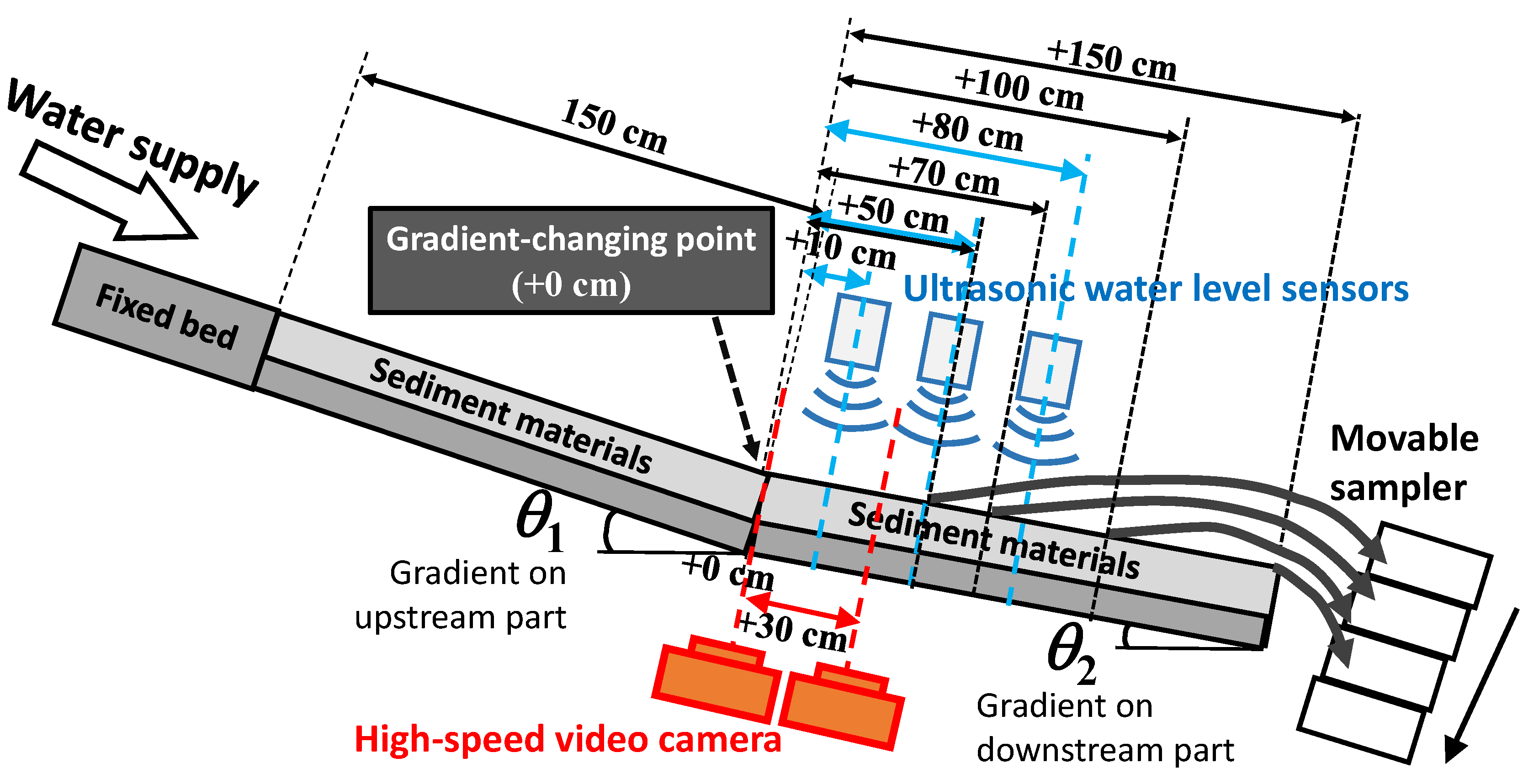
Figure 1 shows the experimental flume and the measurement equipment used in our study. The experimental flume consisted of two variable streambed gradients in the upstream and downstream parts, with lengths of 150 cm and widths of 10 cm, with a fixed bed part for the rectification of the supplied water at the upstream end of the flume. The gradients of the upstream and downstream parts, θ1, θ2, were set to three types; a gentle uniform gradient (θ1 = θ2 = 9°), a steep uniform gradient (θ1 = θ2 = 15°), and a changed gradient (θ1 = 15°, θ2 = 9°). The connecting point of the upstream and downstream parts was defined as the gradient change point (at +0 cm; the positive direction was the downstream side). In addition, the length of the downstream part could be changed to 50 cm, 70 cm, or 100 cm. After the experimental materials were placed at a depth of 5 cm in the upstream and downstream parts (the total material volume including bulks equaled 15,000 cm3), the material was eroded by the supplied water from the upstream end, resulting in the generation of debris flow. We measured the sediment transport concentration of the flow front, , at the downstream end of each length flume (at +50, +80, +100, and +150 cm) using a movable sediment sampler moving in the transverse direction with respect to the flow direction. The sampler separated the debris flow front into the four boxes over the time intervals in the range of 1.0–2.0 s. Measurements were performed to determine the temporal changes in the sediment transport concentrations of the flow front in each sample. We also measured the flow front depths, , using three ultrasonic water level sensors (E4C-DS30, OMRON Corp., Kyoto, Japan) at +10, +50, and +80 cm points, as well as the gravel migration velocities, , in the flow front’s interior using two high-speed video cameras (EXILIM PRO EX-F1, CASIO COMPUTER Co., Ltd., Tokyo, Japan) at +0 and +30 cm points.
The experimental conditions combined with the particle size compositions of the debris flow materials and inflow rates of the supplied water are listed in Table 1. The gravel sizes and debris flow depths of these conditions were set within the gravel size and gravel-size-to-flow-depth ratio ranges used in the previous experiments on debris flow with sediment mixtures performed by Wada et al. [32]. Table 1 also shows the averaged flow depth, flow velocity, Froude number, and particle Reynolds number for the “frontal part” of the debris flow for all cases. In this study, we focused on the effects of the changing gradient on the sediment transport mode at the “frontal part” of the debris flow, whereby the “frontal part” was defined as the part within 3 s from reaching the flow front at a certain measuring point. The magnitude orders of the Froude number and particle Reynolds number were consistent with those of the dimensionless parameters describing previous field and experimental debris flows, as organized by Turnbull et al. [33]. This indicated that our experiments replicated the previous field and experimental debris flows in term of the flow characteristics. The flow velocities on the gentle gradient of the downstream part were greater than those on the steep gradient of the upstream part in many cases. The reason for this may be because the debris flow velocity depends on the magnitude relation regarding the increase or decrease in the streambed gradient and sediment concentration, as shown in Equation (1) below. Under our experimental conditions, the strongest effect on the debris flow velocity is the decreasing sediment concentration rather than the decreasing streambed gradient.
The particle size compositions were prepared by mixing one or two particles of the three particles with diameters of 3.0 mm, 7.1 mm, and 19.0 mm according to the ratios shown in Table 1. The average mass density of these gravel particles (σ) was 2.650 g/cm3, the average concentration in the static sediment bed (C*) was 0.575, and the average internal friction angle () was 34.80°. Here, 80% of the particles in Cases 1–3 were gravel with a diameter of 7.1 mm, while 80% of the particles in Cases 4–6 were gravel with a diameter of 3.0 mm. For all conditions, the inflow rates of the supplied water were set to 1000 and 2000 cm3/s. Note that in Cases 2, 5, and 6, the flow front depth measurements at +10 and +80 cm and the measurements of gravel migration velocities in the flow front interior at +30 cm were not taken, while in Cases 1 and 4, the measurements of sediment transport concentrations of the flow front at +50, +80, and +100 cm were also not taken. This was due to missing or oscillating measurement data caused by a malfunction of the measurement equipment.
In our experiments, no significant topographic changes due to the deposition of debris flow at the gradient change point (+0 cm) occurred during the “frontal part” passing at the point. Therefore, the effects of topographic changes on the transition of sediment transport modes for the “frontal part” were minor.
2.2. Transition Index of Sediment Transport Modes
Using the measurement results, the averaged sediment transport concentration, , the averaged flow depth, , and the vertical averaged gravel migration velocity, , at the “frontal part” of the debris flow were calculated. is calculated using the following equation, using the volumes of water and sediment included in the samples of debris flow fronts obtained by the four boxes in the movable sampler:
where VsLi and VsSi are the coarser and finer sediment volumes included in the samples obtained by the i-th boxes, respectively; Vwi is the water volume included in the samples obtained by the i-th boxes; and i is the number of each box (i = 1–4). Note that in the cases with the debris flow consisting of uniform-sized gravel, VsSi is zero. In the following, , , and in the cases of uniform gradients of 15° and 9° are denoted as , , , , , and , respectively; and , , and in the cases of changing gradients are denoted as , , and at x cm downstream from the gradient change point (+0 cm), respectively. , , and were calculated by averaging the sediment transport concentrations of debris flows obtained by the four samplers. Here, and were the theoretical debris flow depths on the uniform gradients of 15° and 9°, respectively, obtained using the theoretical averaged velocity equation for a stony debris flow as proposed by Takahashi [6] (Equation (2)) and the continuity equation of the flow (Equation (3)). We applied Equation (2) to the consideration of our experimental results because the scales of our experimental conditions were equivalent to Takahashi’s experiments, which were conducted to confirm the equation’s validity [6]. The streambed surface (i.e., the x-coordinate direction that is the basis of Equation (2)) did not change significantly at the gradient change point during the passing point of the “frontal part” in our experiments:
where Um is the vertical averaged velocity of the debris flow, dm is the mean diameter of the material, g is the gravitational acceleration, θ is the streambed gradient, αi is the coefficient (= 0.042), and ρm is the mass density of the interstitial fluid (= 1.0 g/cm3). is the equilibrium sediment concentration from Equation (4), which is derived from the equilibrium of the riverbed shear stress and the body forces of the debris flow on the riverbed in the dynamic equilibrium state of the flow [6]:
where is the averaged measurement value of the flow front depth within 3 s from the time at which the flow front reaches the measuring point; and are the averaged gravel migration velocities within the “median depth” for the theoretical velocity distribution, as suggested by Takahashi et al. [34], for uniform gradients of 15° and 9°, respectively. We defined the “median depth” as the vertical range from to in the interior of the “frontal part”. The theoretical velocity distribution used in this study can be adopted for the velocity distributions of both stony debris and sediment sheet flows (see [34] for details on the theoretical distribution). Note that the internal friction angles (ø) for calculating the theoretical distribution were adjusted according to the experimental results based on the uniform gradients of 15° and 9°. Here, is the averaged measurement value within the “median depth” of the “frontal part”.
Based on the values of the uniform gradients, , , , , , and , and the measurement results for the changing gradient, , , and , the transition indices of sediment transport modes at x cm downstream from the gradient change point (+0 cm point), , , and , were obtained using the following equations:
where , , and are the averaged sediment transport concentration, the theoretical flow depth, and the averaged gravel migration velocities within the “median depth” for the Takahashi’s theoretical velocity distribution [34] at the “frontal part” of the debris flow on a uniform gradient of upstream parts, θ1, respectively. Similarly, , , and are the same indicators on a uniform gradient of downstream parts, θ2, respectively. Using these indices helps us to simply estimate the transition processes of sediment transport modes for any pattern of changed gradients from θ1 to θ2. In this study, we defined θ1 = 15° and θ2 = 9°, and the transition process of the modes on the changed gradients from 15° to 9° were discussed using these indices.
3. Results and Discussion
3.1. Transition of Sediment Transport Modes Based on Changes in Sediment Transport Concentrations of the “Frontal Part” Resulting from Changing Streambed Gradient
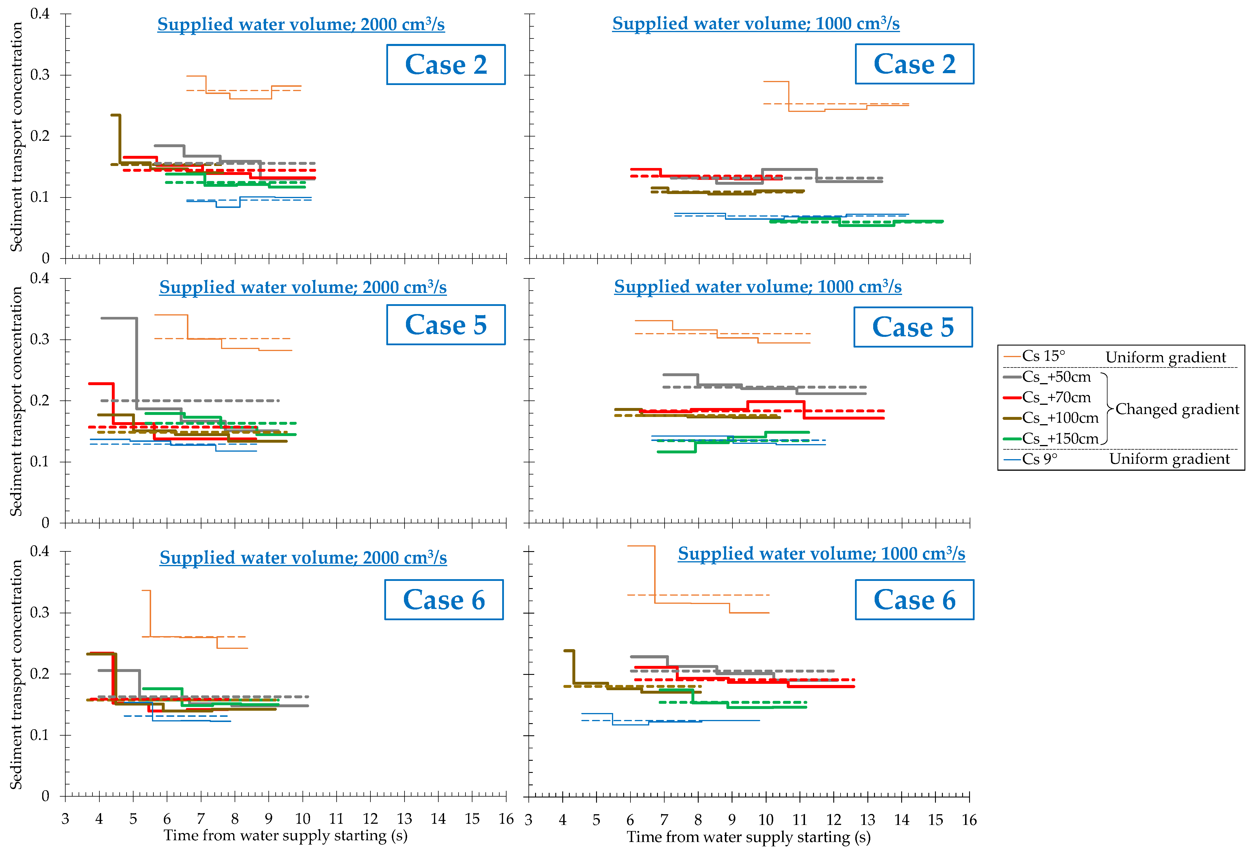
Figure 2 shows the sediment transport concentrations of the “frontal part” of the debris flow,, for all gradient conditions in Cases 2, 5, and 6, respectively. The dotted lines in these figures show the averaged value, , for the sediment transport concentrations of the debris flow obtained by the four samplers. The sediment transport concentrations in the debris flow front, which were obtained by the first sampler, were significant for some cases. This reason for this was that the volumes of gravel in the debris flow front increased more than the interstitial fluid because sufficient clearance between the coarser gravel types in the flow front’s interior was not enough to concentrate the coarser gravel types in the flow front. In the cases with a changing gradient, as the distance between the measuring point and the gradient change point (+0 cm) increased, the sediment transport concentrations became closer to the uniform gradient (9°) for the downstream part. Comparing the results with different inflow rates for each case, although decreased significantly with both inflow rates, these rates were less changed at more than 50 cm downstream from the +0 cm point in the cases where the inflow rates were higher. On the other hand, in the cases where the inflow rates were lower, decreased gradually as the distance from the +0 cm point increased more, and was almost consistent with on the uniform gradient of the downstream part. However, in Case 6 with the finest debris flow material, was larger than , even in the case where the inflow rate was lower. Therefore, in the cases where the inflow rates were higher and the debris flow materials were finer, although decreased significantly over a short distance from the gradient change point (+0 cm), these rates were less changed thereafter. Conversely, in the cases where the inflow rates were lower and the materials were coarser, decreased more as the distance from the gradient change point (+0 cm) increased and was closer to the uniform gradient for the downstream part at +150 cm. These tendencies were confirmed by the averaged sediment transport concentrations of the “frontal part”, , for all cases, as shown in Table 2. This indicates that when the kinetic energy of a debris flow is larger, although some of the flow causes a sudden stoppage (sedimentation) by consuming the kinetic energy because the flow collides with the riverbed near the gradient change point, most of the transported sediment flows downstream because the consumed momentum is less than the total debris flow momentum. Conversely, when the kinetic energy of a debris flow is smaller, although the collision of the flow with the riverbed at the gradient change point is not significant, a firm transition in the sediment transport mode is caused because the materials are unable to maintain their dispersion in the flow’s interior owing to the significant increase in the downward component of gravity on the downstream part.
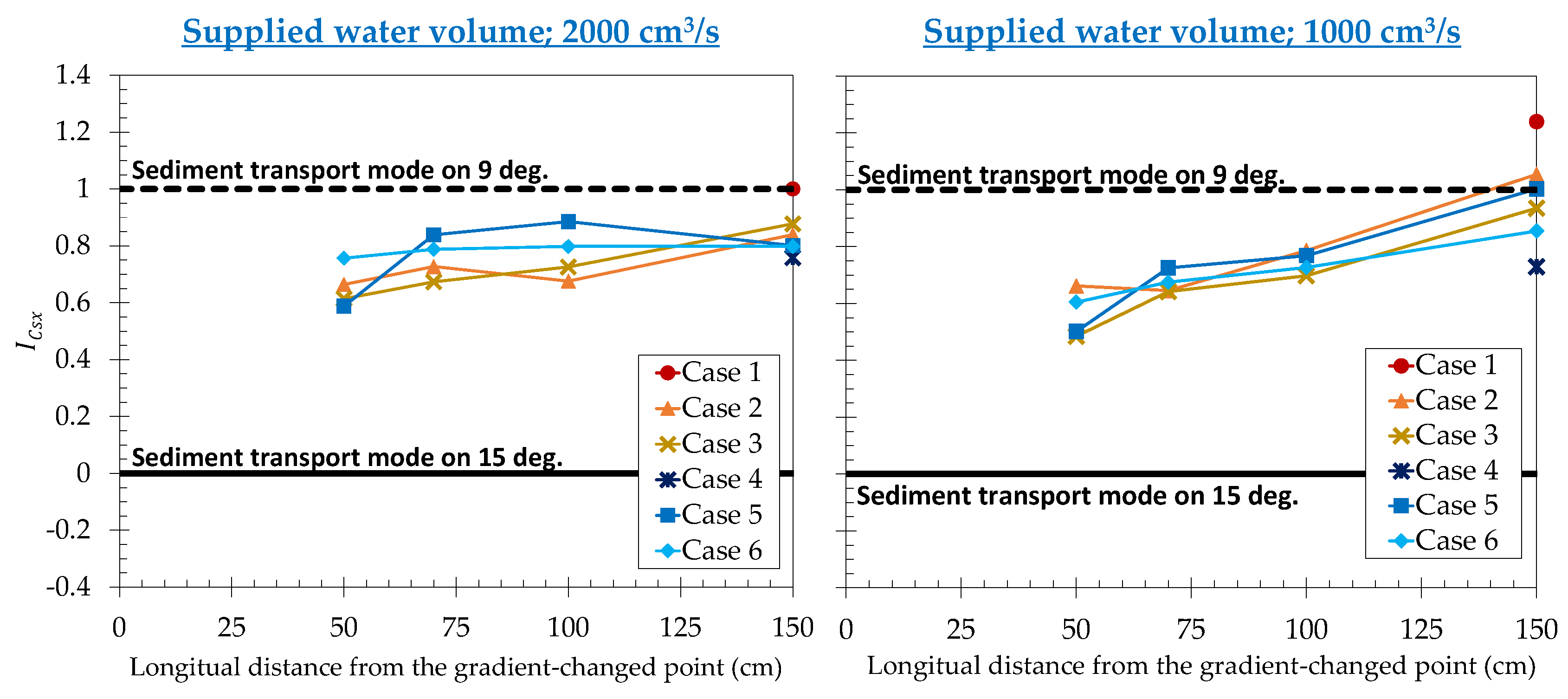
Figure 3 shows the transition indices of sediment transport modes based on the sediment transport concentrations of the “frontal part” of the debris flows, , for all cases at the two inflow rates. Considering that = 0 represents the sediment transport mode at the uniform gradient for the upstream part (15°) and = 1 represents the mode at the uniform gradient for the downstream part (9°), it is considered that as is the closer to 1, the transition to the mode for the downstream parts becomes more significant. The lower the inflow rate, the larger the change in with respect to the increase in the longitudinal distance from the gradient change point (that is, the linear slope of ).
Thus, by using the transition indices, , we can explicitly describe the tendencies mentioned above on sediment transport concentrations of the “frontal part” of the debris flow. However, by using , the similar transition tendencies for all cases (all particle size compositions of debris flow materials) also suggest that the effect of the particle size composition on the transition for sediment transport concentration is relatively small.
3.2. Transition of Sediment Transport Mode Based on Changes in Debris Flow Depths of the “Frontal Part” Resulting from Changing Streambed Gradient
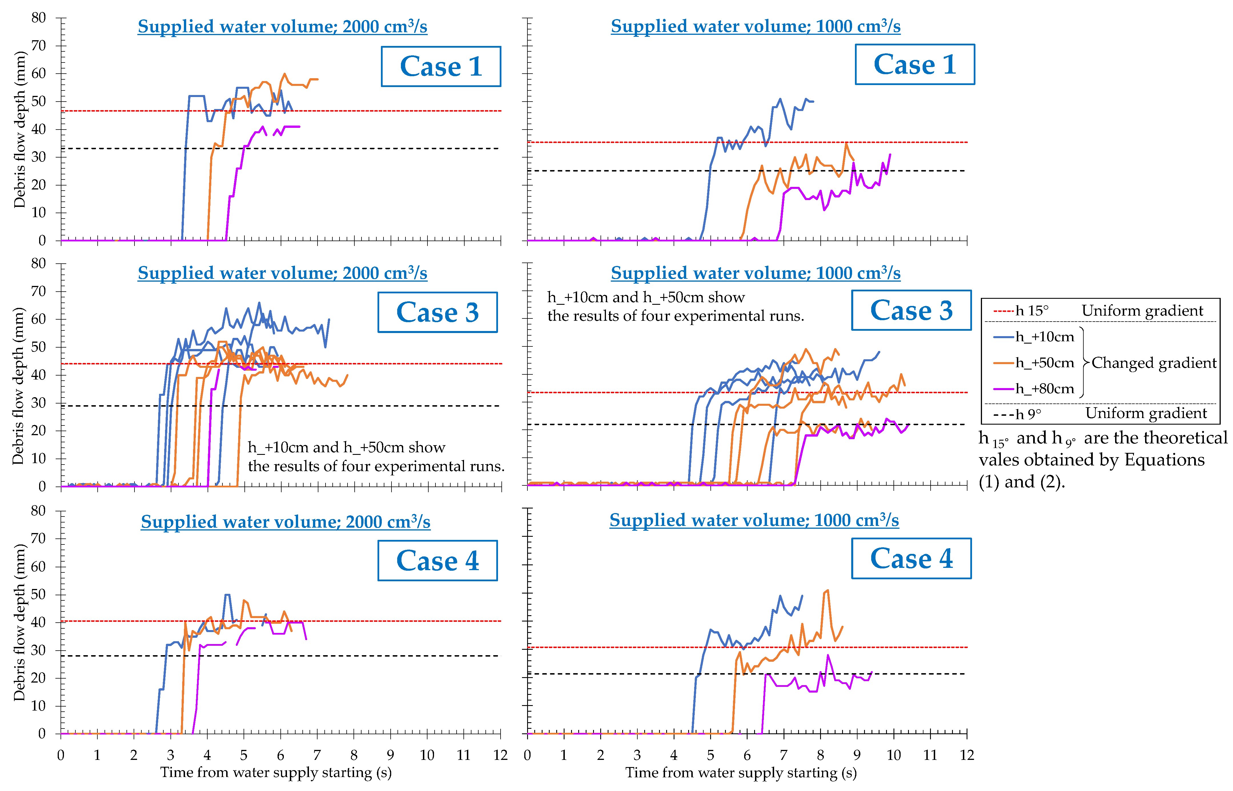
Figure 4 shows the debris flow depths of the “frontal part”,, and the theoretical debris flow depths on the uniform gradients of 15° and 9°, and , for all gradient conditions in Cases 1, 3, and 4, respectively. Even though the sediment transport concentrations of the “frontal part” were significant, the debris flow depths of the “frontal part” did not show remarkable increases for all cases. This may be due to the larger gravel sizes relative to the debris flow depth, whereby the supplied gravel sizes from the subsequent part by riding over the frontal part were few. The measurements of the debris flow depths for several runs in Case 3 generally showed the same trend. This suggested that our experimental results were reproducible.
At 10 cm downstream of the gradient change point, was equal to or greater than the theoretical debris flow depth on the uniform gradient for the upstream part (15°), , with both inflow rates. More than 50 cm downstream from the point, as the distance from the gradient change point to the measuring point increased, was the closer to that on the uniform gradient for the downstream part (9°), . Comparing values for different inflow rates for each case, the values in the cases with the lower inflow rates were closer to than that in the cases with the higher inflow rates. In addition, comparing values in the cases with lower inflow rates, in Case 1 with the coarsest debris flow material was close to , but the values in other cases were close to . Therefore, in the cases where the inflow rates were lower and the debris flow materials were coarser, the closeness of the debris flow depth to the theoretical depth on the uniform gradient for the downstream part was more pronounced as the distance from the gradient change point increased. When flowing at shorter distances from the gradient change point in these cases, the debris flow depths of the “frontal part” were close to . When the kinetic energy of a debris flow is smaller, a firm transition in the sediment transport mode is caused for reasons similar to those for the transitions of sediment transport concentrations by changing gradients; that is, this transition occurs because the materials are unable to maintain their dispersion in the flow’s interior owing to the significant increase in the downward component of gravity on the downstream part. These tendencies were confirmed in the averaged debris flow depths of the “frontal part”, , for all cases, as shown in Table 3.
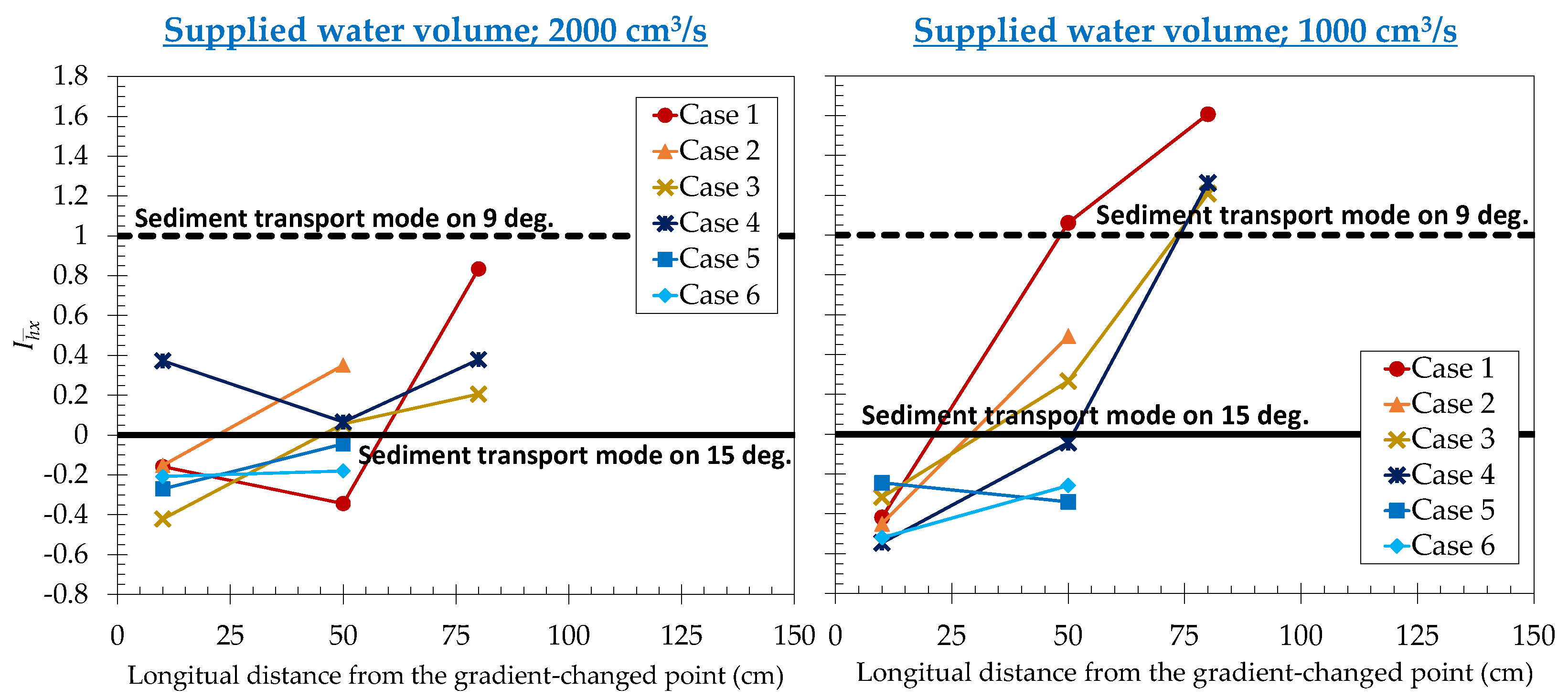
Figure 5 shows the transition indices of sediment transport modes based on debris flow depths of the “frontal part”, , for all cases at the two inflow rates. The lower the inflow rate, the larger the change in with respect to the increase in the longitudinal distance from the gradient change point (that is, the linear slope of ). In addition, in the cases where the inflow rates were lower, as the debris flow materials became coarser, the linear slope of had a greater positive value. Thus, by using the transition indices, , we can explicitly determine the effect of debris flow magnitudes and particle size compositions on the transition for debris flow depths of the “frontal part” by changing the gradient.
3.3. Transition of Sediment Transport Mode Based on Changes in Gravel Migration Velocities in the Interior of the “Frontal Part” Resulting from Changing Streambed Gradient
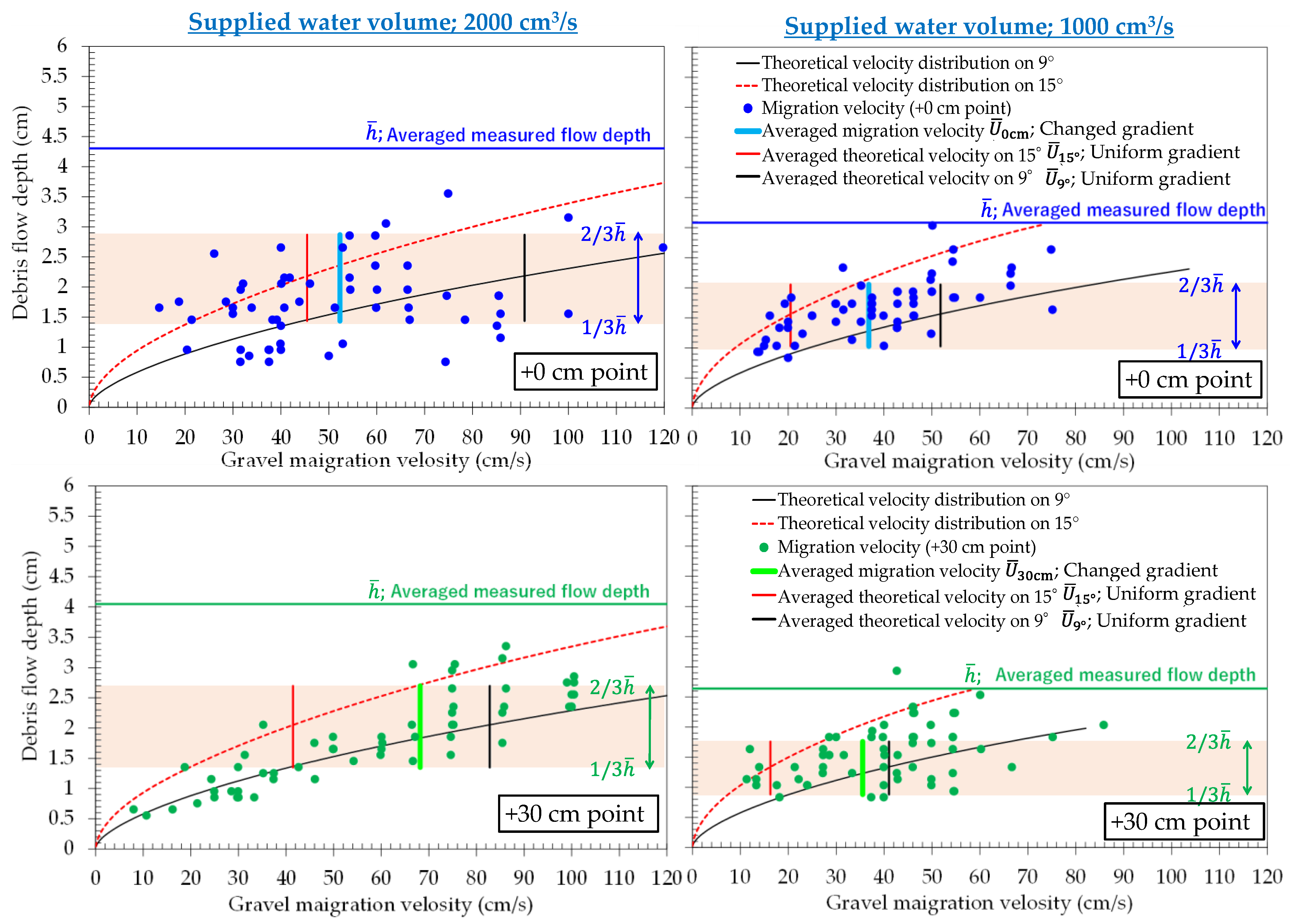
Figure 6 shows the gravel migration velocity distributions in the interior of the “frontal part” of the debris flow in the cases of changing gradients and the theoretical velocity distributions on the uniform gradients of 15° and 9° in Case 3. The flow depths used to obtain these theoretical velocity distributions were the averaged measurement values in the cases of changing gradient. The main parameters used to obtain these distributions, such as the mass density of gravel types (σ), the average concentration in the static sediment bed (C*), and the average internal friction angle (), were identified by trial and error so that the distributions were consistent with the measured distributions on the uniform gradients of 15° and 9° in Case 2 (see Figure 7). This figure also shows the averaged measured velocities within the “median depth” of the “frontal part”, , and the averaged theoretical velocities within the “median depth”, and . As the debris flows flowed over longer distances from the gradient change point, became closer to the theoretical velocities on the uniform gradient of the downstream part, . In the cases where the inflow rates were lower, these tendencies were more pronounced. These trends were the similar to the aforementioned transition trends of the sediment transport concentrations and flow depths. Therefore, the transition mechanisms of the gravel migration velocities resulting from the changing gradient were estimated to be similar to the aforementioned mechanism. These tendencies were confirmed in the averaged measurement velocities within the “median depth” of the “frontal part”, , for all cases where the inflow rates were lower, as shown in Table 4. However, in the cases where the inflow rates were higher, these tendencies were not pronounced for all cases, and in some cases there was a significant decrease in near the gradient change point. The reason for this was the same as the aforementioned reason for the transition of the sediment transport concentrations. In other words, these tendencies indicated that although a part of the flow causes a sudden stop (sedimentation) by consuming the kinetic energy when the flow collides with the riverbed near the gradient change point, most of the transported sediment flows downstream because the consumed momentum is less than the total debris flow momentum.
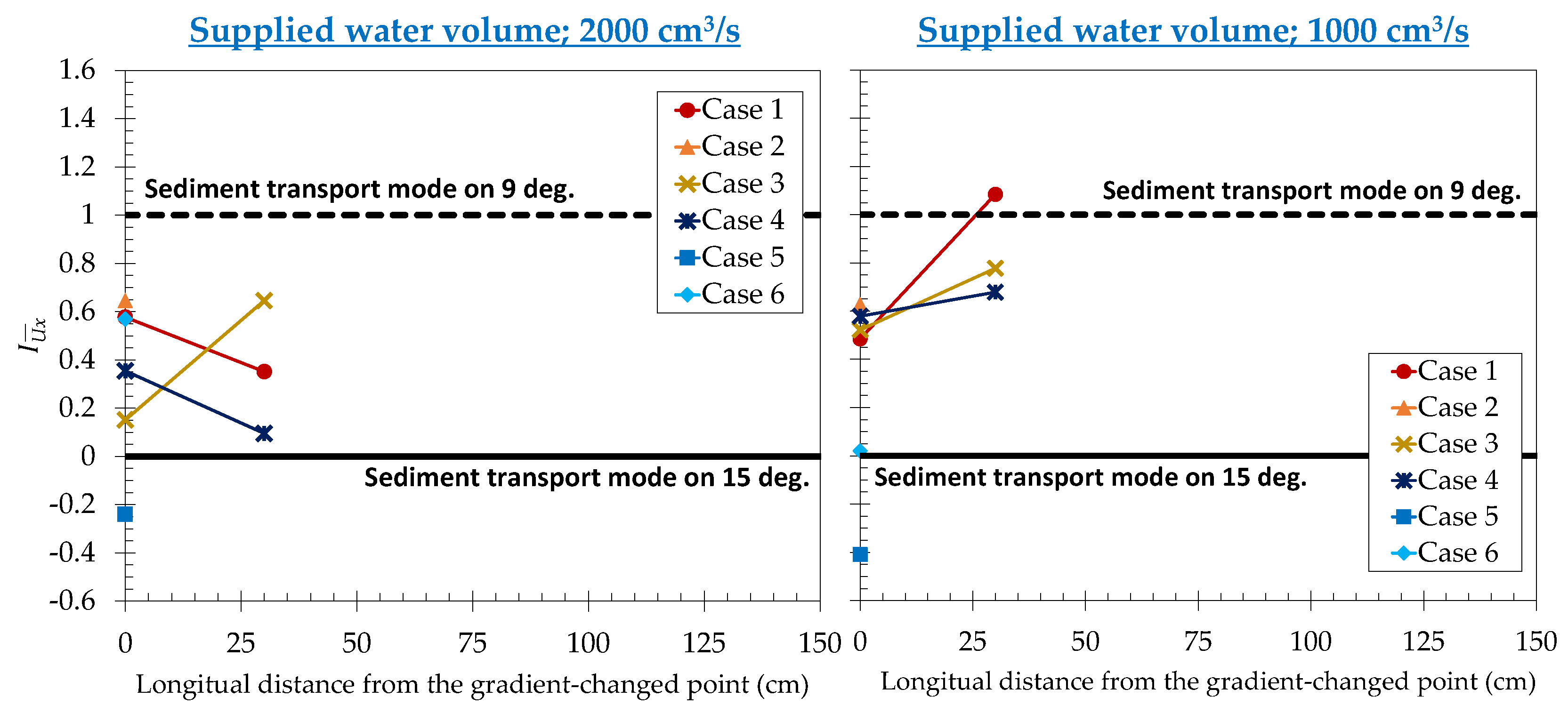
Figure 8 shows the transition indices of sediment transport modes based on the averaged gravel migration velocities within the “median depth” of the “frontal part”, , for all cases at the two inflow rates. In the case with the lower inflow rate, the linear slope of was significantly positive. This demonstrates that as the debris flows flowed greater distances from the gradient change point, the front velocities were closer to the theoretical velocities on the uniform gradient of the downstream part for all cases. Conversely, in the cases with the higher inflow rate, no clear trend common to all cases is observed because the linear slope of is not monotonic. The possible reason for this is that a part of the flow causes a sudden stop (sedimentation) by consuming of their kinetic energy because the flow collides with the riverbed near the gradient change point. Thus, by using the transition indices, , we can explicitly determine the effect of debris flow magnitudes on the transition for migration velocities in the interior of the “frontal part” by changing the gradient. However, it is necessary to confirm the validity of the transition indices for other pattern of changed gradients, except for the changed gradients from 15° to 9°.
3.4. Estimation of Transition Processes of Sediment Transport Modes Resulting from Changing Streambed Gradient Based on Transition Indices
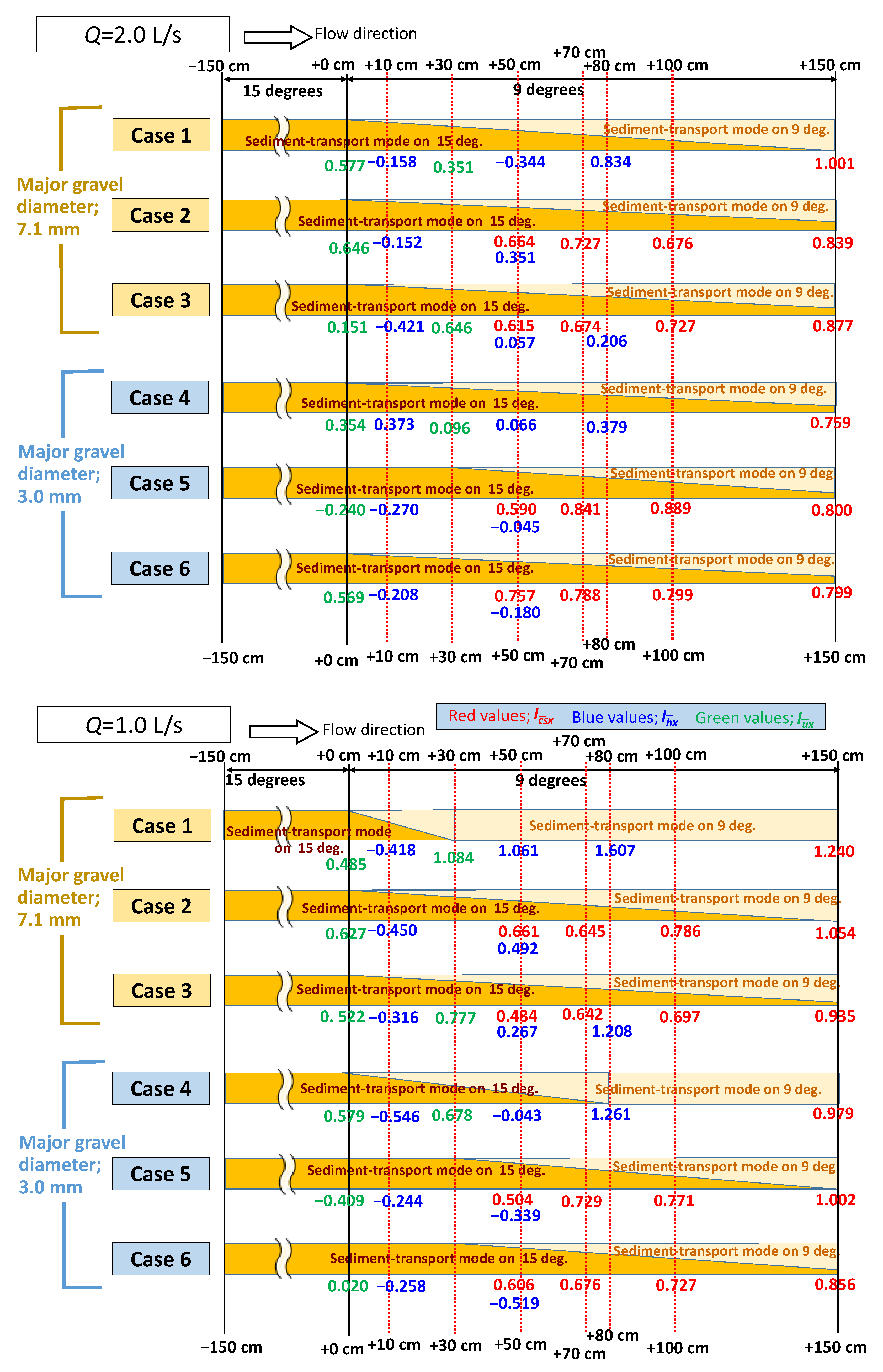
Based on the transition indices at all measurement points in all cases and shown in Section 3.1 to Section 3.3, the transition processes of sediment transport modes for all cases were estimated, as shown in Figure 9. The transitions of sediment transport modes of the “frontal part” occurred in the section from the gradient change point (+0 cm) to +150 cm in all cases. In the cases where the inflow rates were higher or the debris flow materials were finer (i.e., the kinetic energies of the debris flow were larger), the transition was not completed at +150 cm. The materials of the debris flow with larger kinetic energy were considered to be able to maintain their dispersion in the flow interior after passing the gradient change point owing to sufficient debris flow momentum. Conversely, when the kinetic energies were smaller, the transition was completed in the shorter longitudinal transition sections. Therefore, it is important to investigate the major gravel sizes and flow magnitudes of debris flows to understand the transition processes of sediment transport modes of debris flow with various particle size compositions owing to the changes in gradient.
Comparing the longitudinal trends of the three transition indices based on the sediment transport concentrations, flow depths, and gravel migration velocities of the “frontal part”, with , , and at the downstream part, it is suggested that significantly increases immediately after passing the gradient change point. On the other hand, changes most slowly. Therefore, it is inferred that the transition process of sediment transport modes resulting from changing streambed gradients is as follows. First, the changing streambed gradient causes a rapid decrease in the migration velocities for some of the gravel in the interior of the debris flow. This leads to a decrease in the sediment transport concentration. This decreases opportunities for collisions and decreases the friction of the debris flow materials in the flow interior, leading to a decrease in energy dissipation; therefore, the debris flow depth decreases. These stepwise order of the changes in hydraulic quantities is not considered in the theoretical laws of the conventional debris flow [6,7,8,9,10,11,12,13,14,15,16]. Therefore, the transition indices provide important findings regarding the transition of sediment transport modes due to changing gradients. However, as Zordan et al. [35] suggested, the stepwise order depends on the interaction between the changing debris flow mechanism and the streambed changes at the gradient change point. Therefore, future studies are required that focus on this interaction at the gradient change point using experimental measurements of the changing hydrodynamic quantities, such as the streambed shear stress measurements [35], as well as studies on the mechanistic approaches using the constitutive laws of the debris flow with a gradient-independent global coordinate system [22,23] or numerical approaches with the two-layer flow model or moving particle semi-implicit (MPS) method [24,25].
4. Conclusions
In this study, using an experimental flume with two variable gradients in the upstream and downstream parts, we investigated the transition processes of sediment transport modes in debris flows composed of materials of various particle sizes owing to the changes in streambed gradients. In our discussion of the transition processes along the longitudinal distances from the gradient change point, the transition indices , , and were used. These were calculated based on measurements of sediment transport concentrations, flow depths, and gravel migration velocities in debris flow fronts in the downstream part. The findings of this study are as follows:
- After a debris flow passes the gradient change point, the transition of the sediment transport modes progresses by changing the sediment transport concentrations, flow depths, and gravel migration velocities to those in the steady-state condition on the gradient of the downstream part;
- In the cases where the debris flow magnitudes are higher and the materials are finer—that is, the kinetic energies are larger—a part of the flow will cause a sudden stop (sedimentation) because the flow will collide with the riverbed near the gradient change point. However, the transition of the sediment transport modes is less pronounced because the dispersion of the debris flow material in the flow interior is maintained after passing the gradient change point owing to the sufficient debris flow momentum. Conversely, in the cases where the inflow rates are lower and the materials are coarser, the transition is more pronounced when flowing at shorter distances from the gradient change point. Therefore, it is important to investigate the major gravel sizes and flow magnitudes of debris flows to understand the transition processes caused by the changing streambed gradient;
- By using the three transition indices, , , and , we can explicitly determine the effects of debris flow magnitudes and their particle size compositions on the transition processes by changing the gradient. However, it is necessary to confirm the validity of the transition indices for other patterns of changed gradients, except for the gradients that change from 15° to 9°;
- increases significantly immediately after passing the gradient change point. In contrast, changes most slowly. Therefore, the transition process of sediment transport modes resulting from changing streambed gradients occurs as follows. First, the changed streambed gradient causes a rapid decrease in the migration velocities of some gravel types in the interior of the debris flow. This leads to a decrease in the sediment transport concentration. This decreases opportunities for collisions and decreases the friction of the debris flow materials in the flow interior, leading to a decrease in energy dissipation. Therefore, the debris flow depth decreases.
Our future tasks include applying the proposed concept and indices for the transition of the modes under the various conditions in terms of gradient change patterns, the flow magnitudes, and the particle size compositions of the debris flow to investigate the validity of the three transition indices, as well as to consider a general transition index that is suitable for assessing the transition under various conditions.
Author Contributions
Conceptualization, T.W. and H.M. (Hiroshi Miwa); methodology, T.W., H.M. (Hirotada Mishima), J.T., and K.K.; validation, T.W. and H.M. (Hiroshi Miwa); formal analysis, T.W. and H.M. (Hiroshi Miwa); investigation, T.W., H.M. (Hirotada Mishima), J.T., and K.K.; data curation, T.W., H.M. (Hirotada Mishima), J.T., and K.K.; writing—original draft preparation, T.W., H.M. (Hirotada Mishima), J.T., and K.K.; writing—review and editing, T.W. and H.M. (Hiroshi Miwa); visualization, T.W., H.M. (Hirotada Mishima), J.T., and K.K.; supervision, T.W. and H.M. (Hiroshi Miwa); funding acquisition, T.W. and H.M. (Hiroshi Miwa). All authors have read and agreed to the published version of the manuscript.
Funding
This research was funded by JSPS KAKENHI Grant-in-Aid for Young Scientists, Grant Number 22K14454, and Research Grants from the Electric Technology Research Foundation of Chugoku (Grant Subject: Development of a Numerical Model for Deposition Trend in a Dam Reservoir Considering the Spatial and Temporal Distribution and Transport Processes of Various Sized Sediment Production in the Dam Reservoir Catchment).
Data Availability Statement
Not applicable.
Acknowledgments
Our great thanks go to Yasuhito Takeuchi for his aid in the conception and creation of our experimental flume.
Conflicts of Interest
The authors declare no conflict of interest.
References
- Wang, F.; Wu, Y.H.; Yang, H.; Tanida, Y.; Kamei, A. Preliminary investigation of the 20 August 2014 debris flows triggered by a severe rainstorm in Hiroshima City, Japan. Geoenviron. Disasters 2015, 2, 17. [Google Scholar] [CrossRef] [Green Version]
- Hashimoto, R.; Tsuchida, T.; Moriwaki, T.; Kano, S. Hiroshima Prefecture geo-disasters due to Western Japan Torrential rainfall in July 2018. Soils Found 2020, 60, 283–299. [Google Scholar] [CrossRef]
- Gong, X.L.; Chen, K.T.; Chen, X.Q.; You, Y.; Chen, J.G.; Zhao, W.Y.; Lang, J. Characteristics of a Debris Flow Disaster and Its Mitigation Countermeasures in Zechawa Gully, Jiuzhaigou Valley, China. Water 2020, 12, 1256. [Google Scholar] [CrossRef]
- Rosli, M.I.; Che Ros, F.; Razak, K.A.; Ambran, S.; Kamaruddin, S.A.; Nor Anuar, A.; Marto, A.; Tobita, T.; Ono, Y. Modelling Debris Flow Runout: A Case Study on the Mesilau Watershed, Kundasang, Sabah. Water 2021, 13, 2667. [Google Scholar] [CrossRef]
- Wada, T.; Kodani, R.; Miwa, H. Spatial analysis on occurrence factors of multiple slope failures using topographic and rainfall indices with high spatial resolutions. Int. J. GEOMATE 2021, 20, 89–97. [Google Scholar] [CrossRef]
- Takahashi, T. Mechanical characteristics of debris flow. J. Hydraul. Div. Proc. Am. Soc. Civ. Eng. 1978, 104, 1153–1169. [Google Scholar] [CrossRef]
- Savage, S.B. Gravity flow of cohesionless granular materials in chutes and channels. J. Fluid Mech. 1979, 92, 53–96. [Google Scholar] [CrossRef]
- Tsubaki, T.; Hashimoto, H.; Suetsugi, T. Grain stresses and flow properties of debris flow. Proc. Jpn. Soc. Civ. Eng. 1982, 317, 70–91. (In Japanese) [Google Scholar] [CrossRef] [Green Version]
- Chen, C.L. Generalized viscoplastic modeling of debris flow. J. Hydraul. Eng. 1986, 114, 237–257. [Google Scholar] [CrossRef]
- Egashira, S.; Miyamoto, K.; Itoh, T. Constitutive equations of debris flow and their applicability. In Proceedings of the 1st International Conference on Debris Flow Hazards Mitigation, San Francisco, CA, USA, 7–9 August 1997; pp. 340–349. [Google Scholar]
- Takahashi, T. Study on the deposition of debris flows (3); Erosion of debris fan. Disaster Prev. Res. Inst. Annu. Kyoto Univ. 1982, 25, 327–348, (In Japanese with English abstract). [Google Scholar]
- Hashimoto, H.; Tsubaki, T.; Hirano, M. Sediment Gravity Flow on Relatively Gentle Slopes. Annu. J. Hydraul. Eng. Jpn. Soc. Civ. Eng. 1986, 30, 235–240. (In Japanese) [Google Scholar]
- Takahashi, T. High velocity flow in steep erodible channels. In Proceedings of the 22nd IAHR Congress, Lausanne, Switzerland, 31 August–4 September 1987; pp. 42–53. [Google Scholar]
- Ashida, K.; Takahashi, T.; Mizuyama, T. Study on bed load equations for mountain streams. J. Jpn. Soc. Eros. Control Eng. 1978, 30, 9–17, (In Japanese with English abstract). [Google Scholar]
- Egashira, S.; Ashida, K.; Takahama, J.; Tanonaka, S. Sediment transport formula derived from an energy dissipation model of solid-fluid mixture. Disaster Prev. Res. Inst. Annu. Kyoto Univ. 1990, 33, 293–306, (In Japanese with English abstract). [Google Scholar]
- Mizuyama, T. Sediment transport rate in the transition region between debris flow and bed load transport. J. Jpn. Soc. Eros. Control Eng. 1980, 33, 1–6, (In Japanese with English abstract). [Google Scholar]
- Iverson, R.M.; Logan, M.; LaHusen, R.G.; Berti, M. The perfect debris flow? Aggregated results from 28 large-scale experiments. J. Geophys. Res. 2010, 115, F03005. [Google Scholar] [CrossRef]
- Cheng, Y.M.; Fung, I.W.H.; Li, L.; Li, N. Laboratory and Field Test and Distinct Element Analysis of Dry Granular Flows and Segregation Processes. Nat. Hazards Earth Syst. Sci. 2019, 19, 181–199. [Google Scholar] [CrossRef] [Green Version]
- Chen, Z.; Yang, P.; Liu, H.; Zhang, W.; Wu, C. Characteristics analysis of granular landslide using shaking table model test. Soil Dyn. Earthq. Eng. 2019, 126, 105761. [Google Scholar] [CrossRef]
- Takahashi, T.; Nakagawa, H.; Kuang, S. Estimation of debris flow hydrograph on varied slope bed, Erosion and Sedimentation in the Pacific Rim. In Proceedings of the Corvallis Symposium, Corvallis, OR, USA, 3–7 August 1987; Volume 165, pp. 167–177. [Google Scholar]
- Ikeda, A.; Mizuyama, T.; Sugiura, N.; Hasegawa, Y. Study about deformation of stream bed deposit at initiation zone of debris flow. J. Jpn. Soc. Eros. Control Eng. 2009, 62, 46–51, (In Japanese with English abstract). [Google Scholar]
- Juez, C.; Soares-Frazao, S.; Murillo, J.; García-Navarro, P. Experimental and numerical simulation of bed load transport over steep slopes. J. Hydraul. Res. 2017, 55, 455–469. [Google Scholar] [CrossRef]
- Veronica, C.; Petrie, j.; Timbe, L.; Pacheco, E.; Astudillo, W.; Padilla, C.; Cisneros, F. Validation of an Experimental Procedure to Determine Bedload Transport Rates in Steep Channels with Coarse Sediment. Water 2021, 13, 672. [Google Scholar]
- Takahama, J.; Fujita, Y.; Kondo, Y.; Hachiya, K. A two layer simulation model unifying debris flow and sediment sheet flow. In Proceedings of the International Congress INTERPRAEVENT 2002 in the Pacific Rim, Matsumoto, Japan, 14–18 October 2002; pp. 113–124. [Google Scholar]
- Suzuki, T.; Hotta, N. Development of Modified Particles Method for Simulation of Debris Flow Using Constitutive Equations. Int. J. Eros. Control Eng. 2016, 9, 165–173. [Google Scholar] [CrossRef] [Green Version]
- Sharp, R.P.; Nobles, L.H. Mudflow of 1941 at Wrightwood, southern California. Bull. Geol. Soc. Am. 1953, 64, 547–560. [Google Scholar] [CrossRef]
- Curry, R.R. Observation of Alpine Mudflows in the Tenmile Range, Central Colorado. Bull. Geol. Soc. Am. 1966, 77, 771–776. [Google Scholar] [CrossRef]
- Okuda, S.; Suwa, H.; Okunishi, K.; Nakano, M.; Yokoyama, K. Synthetic observation on debris flow part. 3, Observation at valley Kamikamihorisawa of Mt. Yakedake. Disaster Prev. Res. Inst. Annu. Kyoto Univ. 1977, 20, 237–263, (In Japanese with English abstract). [Google Scholar]
- Ishikawa, Y. Debris flow in the Name river. J. Jpn. Soc. Eros. Control Eng. 1985, 37, 24–29. (In Japanese) [Google Scholar]
- Teramoto, Y.; Jitousono, T.; Shimoyama, E. Flow properties of the debris flow that occurred on September 11, 1999, in the Akamatsu-dani River Basin at Unzen Volcano. Res. Bull. Kagoshima Univ. Forests. 2002, 30, 19–25, (In Japanese with English abstract). [Google Scholar]
- Gray, J.M.N.T.; Kokelaar, B.P. Large particle segregation, transport and accumulation in granular freesurface flows. J. Fluid Mech. 2010, 652, 105–137. [Google Scholar] [CrossRef]
- Wada, T.; Furuya, T.; Nakatani, K.; Mizuyama, T.; Satofuka, Y. Experimental Study on the Concentration of Coarser Particles at the Frontal Segment of a Debris Flow. Int. J. Eros. Control Eng. 2015, 8, 20–30. [Google Scholar] [CrossRef] [Green Version]
- Turnbull, B.; Bowman, E.T.; McElwaine, J.N. Debris flows: Experiments and modelling. Comptes Rendus Physique 2015, 16, 86–96. [Google Scholar] [CrossRef]
- Takahashi, T.; Satofuka, Y.; Chishiro, K. Dynamical law of debris flows in inertial regime. Disaster Prev. Res. Inst. Annu. Kyoto Univ. 1996, 39, 333–346, (In Japanese with English abstract). [Google Scholar]
- Zordan, J.; Juez, C.; Schleiss, A.J.; Franca, M.J. Entrainment, transport and deposition of sediment by saline gravity currents. Adv. Water Resour. 2018, 115, 17–32. [Google Scholar] [CrossRef]
Figure 1.
Experimental setup.

Figure 2.
Time variations in sediment transport concentrations of the “frontal part” of the debris flow, , for all gradient conditions in Cases 2, 5, and 6.
Figure 2.
Time variations in sediment transport concentrations of the “frontal part” of the debris flow, , for all gradient conditions in Cases 2, 5, and 6.

Figure 3.
Transition indices of sediment transport modes based on sediment transport concentrations of the “frontal part” of the debris flow, , for all cases with two inflow rates.
Figure 3.
Transition indices of sediment transport modes based on sediment transport concentrations of the “frontal part” of the debris flow, , for all cases with two inflow rates.

Figure 4.
Time variations in debris flow depths of the “frontal part” of the debris flow, , for all gradient conditions in Cases 1, 3, and 4.
Figure 4.
Time variations in debris flow depths of the “frontal part” of the debris flow, , for all gradient conditions in Cases 1, 3, and 4.

Figure 5.
Transition indices of sediment transport modes based on flow depths of the “frontal part” of the debris flow, , for all cases with two inflow rates.
Figure 5.
Transition indices of sediment transport modes based on flow depths of the “frontal part” of the debris flow, , for all cases with two inflow rates.

Figure 6.
Measured gravel velocity distributions in the interior of the “frontal part” of the debris flow in the cases involving a changing gradient and theoretical velocity distributions on uniform gradients of 9°and 15° for Case 3.
Figure 6.
Measured gravel velocity distributions in the interior of the “frontal part” of the debris flow in the cases involving a changing gradient and theoretical velocity distributions on uniform gradients of 9°and 15° for Case 3.

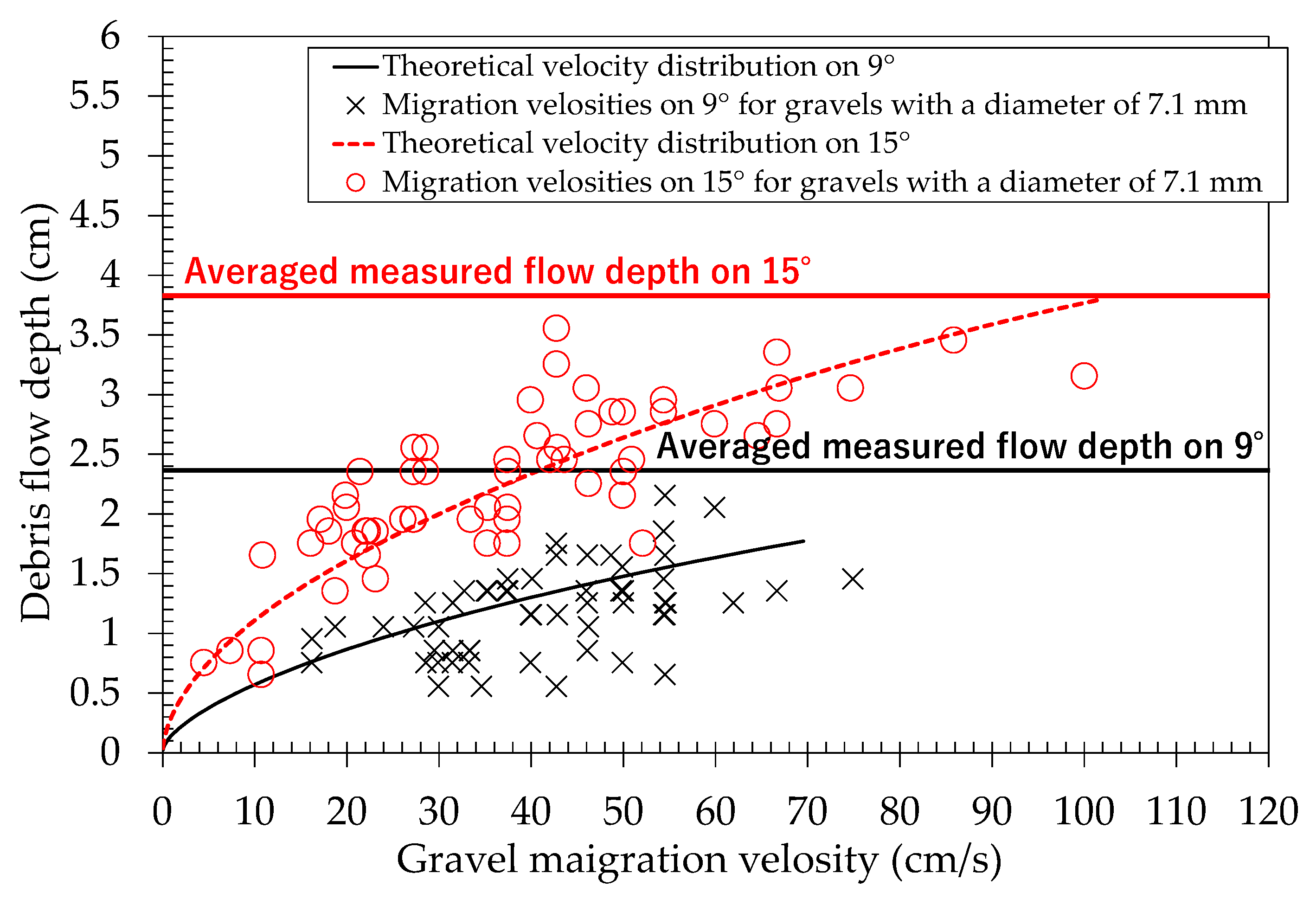
Figure 7.
Comparison of theoretical velocity distribution as suggested by Takahashi et al. [34] and measured migration velocities for case 2 on uniform gradients of 15° and 9°. The main parameters used to obtain the theoretical velocity distribution were the mass density of gravel (σ) = 2650 kg/m3, internal friction angle (ø) = 32°, and concentration in the static sediment bed (C*) = 0.650.

Figure 8.
Transition indices of sediment transport modes based on averaged gravel migration velocities within the “median depth” in the interior of the “frontal part” of the debris flow, , for all cases with two inflow rates.
Figure 8.
Transition indices of sediment transport modes based on averaged gravel migration velocities within the “median depth” in the interior of the “frontal part” of the debris flow, , for all cases with two inflow rates.

Figure 9.
Estimated longitudinal transition processes of sediment transport modes of the “frontal part” of the debris flow for all cases, based on the transition indices. Red, blue, and green values in the figure are the transition indices of sediment transport modes at x cm downstream from the gradient change point for the sediment transport concentration, the averaged flow depth, and the vertical averaged gravel migration velocities at the “frontal part” of the debris flow, i.e., , , and .


Table 1.
Experimental cases and conditions.
| Case | Debris Flow Composition | Inflow Rate 2 (cm3/s) | Flume Gradient 2 θ1, θ2 (°) 3 | Measured Representative Values of the “Frontal Part” 4 of a Debris Flow with a Changing Gradient | |||||
|---|---|---|---|---|---|---|---|---|---|
| dL, dS (mm) 1 | PL, PS1 | Condition | (mm) | (mm/s) | Frf 7 | Re*f 8 | |||
| Case 1 | 19.0, 7.1 | 20%, 80% | 2000 1000 | Gentle uniform gradient 9°, 9° Steep uniform gradient 15°, 15° Changed gradient 15°, 9° | Inflow rate; 2000 cm3/s | ||||
| Upstream part (15°) | 29.767 | 545.45 | 1.028 | 2651.78 | |||||
| Downstream part (9°) | 51.300 | 571.43 | 0.811 | 2676.44 | |||||
| Inflow rate; 1000 cm3/s | |||||||||
| Upstream part (15°) | 30.000 | 260.87 | 0.489 | 2662.13 | |||||
| Downstream part (9°) | 24.533 | 363.64 | 0.746 | 1850.86 | |||||
| Case 2 | 7.1, non | 100%, 0% | Inflow rate; 2000 cm3/s | ||||||
| Upstream part (15°) | 29.567 | 315.79 | 0.597 | 1979.35 | |||||
| Downstream part (9°) | 40.453 | 615.38 | 0.983 | 1780.02 | |||||
| Inflow rate; 1000 cm3/s | |||||||||
| Upstream part (15°) | 27.667 | 321.43 | 0.628 | 1914.70 | |||||
| Downstream part (9°) | 29.008 | 387.10 | 0.730 | 1507.33 | |||||
| Case 3 | 7.1, 3.0 | 80%, 20% | Inflow rate; 2000 cm3/s | ||||||
| Upstream part (15°) | 36.000 | 387.10 | 0.663 | 1931.84 | |||||
| Downstream part (9°) | 43.250 | 615.38 | 0.951 | 1627.96 | |||||
| Inflow rate; 1000 cm3/s | |||||||||
| Upstream part (15°) | 24.000 | 285.71 | 0.599 | 1577.34 | |||||
| Downstream part (9°) | 30.367 | 390.24 | 0.719 | 1364.12 | |||||
| Case 4 | 19.0, 3.0 | 20%, 80% | Inflow rate; 2000 cm3/s | ||||||
| Upstream part (15°) | 28.700 | 545.45 | 1.046 | 1702.92 | |||||
| Downstream part (9°) | 39.767 | 571.43 | 0.921 | 1541.15 | |||||
| Inflow rate; 1000 cm3/s | |||||||||
| Upstream part (15°) | 19.867 | 500.00 | 1.152 | 1416.83 | |||||
| Downstream part (9°) | 31.167 | 363.64 | 0.662 | 1364.36 | |||||
| Case 5 | 7.1, 3.0 | 20%, 80% | Inflow rate; 2000 cm3/s | ||||||
| Upstream part (15°) | 31.667 | 375.00 | 0.685 | 1102.11 | |||||
| Downstream part (9°) | 38.033 | 888.89 | 1.464 | 928.61 | |||||
| Inflow rate; 1000 cm3/s | |||||||||
| Upstream part (15°) | 19.200 | 181.82 | 0.426 | 858.17 | |||||
| Downstream part (9°) | 31.858 | 545.45 | 0.982 | 849.89 | |||||
| Case 6 | 3.0, non | 100%, 0% | Inflow rate; 2000 cm3/s | ||||||
| Upstream part (15°) | 21.333 | 510.64 | 1.136 | 710.41 | |||||
| Downstream part (9°) | 36.747 | 727.27 | 1.219 | 716.84 | |||||
| Inflow rate; 1000 cm3/s | |||||||||
| Upstream part (15°) | 23.100 | 276.92 | 0.592 | 739.24 | |||||
| Downstream part (9°) | 28.600 | 631.58 | 1.120 | 632.40 | |||||
Note: 1 d1 and d2 are the diameters of coarser and finer gravel types, respectively; P1 and P2 are the initial compositions of coarser and finer gravel types, respectively; 2 common conditions in all cases; 3 θ1 and θ2 are the gradients of the upstream and downstream parts in the experimental flume, respectively; 4 “frontal part” is the part within 3 s from reaching the flow front at a certain measuring point; 5 is the averaged flow depth at the “frontal part” of a debris flow; 6 is the averaged front velocity of a debris flow in the section from 50 cm upstream from the gradient change point to 50 cm downstream from the point; 7 Frf is the Froude number, = , where is the gravitational acceleration, 9.81 × 102 mm/s2; 8 Re*f is the particle Reynolds number, =, where dm is the mean diameter of the debris flow material and is the kinematic viscosity coefficient, 1.00 mm2/s.
Table 2.
Averaged sediment transport concentrations of the “frontal part” of the debris flow, , for all cases with two inflow rates.
Table 2.
Averaged sediment transport concentrations of the “frontal part” of the debris flow, , for all cases with two inflow rates.
| Case | Inflow Rate (cm3/s) | ||||||
|---|---|---|---|---|---|---|---|
| Case 1 | 2000 | 0.260 | - | - | - | 0.124 | 0.124 |
| Case 2 | 0.275 | 0.156 | 0.144 | 0.154 | 0.124 | 0.096 | |
| Case 3 | 0.250 | 0.164 | 0.156 | 0.148 | 0.127 | 0.110 | |
| Case 4 | 0.272 | - | - | - | 0.170 | 0.138 | |
| Case 5 | 0.302 | 0.200 | 0.157 | 0.149 | 0.163 | 0.129 | |
| Case 6 | 0.261 | 0.163 | 0.159 | 0.158 | 0.158 | 0.132 | |
| Case 1 | 1000 | 0.256 | - | - | - | 0.013 | 0.060 |
| Case 2 | 0.253 | 0.132 | 0.135 | 0.109 | 0.060 | 0.070 | |
| Case 3 | 0.256 | 0.161 | 0.131 | 0.120 | 0.073 | 0.061 | |
| Case 4 | 0.318 | - | - | - | 0.130 | 0.060 | |
| Case 5 | 0.310 | 0.222 | 0.183 | 0.176 | 0.135 | 0.136 | |
| Case 6 | 0.330 | 0.206 | 0.191 | 0.181 | 0.154 | 0.125 |
Table 3.
Averaged debris flow depths of the “frontal part”, , and theoretical debris flow depths on the uniform gradients, and , for all cases with two inflow rates (unit; mm).
Table 3.
Averaged debris flow depths of the “frontal part”, , and theoretical debris flow depths on the uniform gradients, and , for all cases with two inflow rates (unit; mm).
| Case | Inflow Rate (cm3/s) | |||||
|---|---|---|---|---|---|---|
| Case 1 | 2000 | 46.670 | 48.800 | 51.300 | 35.429 | 33.198 |
| Case 2 | 45.871 | 48.217 | 40.453 | — | 30.446 | |
| Case 3 | 44.104 | 50.458 | 43.250 | 41.000 | 29.008 | |
| Case 4 | 40.589 | 35.917 | 39.767 | 35.846 | 28.078 | |
| Case 5 | 37.428 | 41.100 | 38.033 | — | 23.845 | |
| Case 6 | 34.447 | 37.100 | 36.747 | — | 21.674 | |
| Case 1 | 1000 | 35.369 | 39.633 | 24.533 | 18.967 | 25.159 |
| Case 2 | 34.764 | 40.022 | 29.008 | — | 23.074 | |
| Case 3 | 33.424 | 37.042 | 30.367 | 19.600 | 21.984 | |
| Case 4 | 30.760 | 35.933 | 31.167 | 18.800 | 21.279 | |
| Case 5 | 28.365 | 30.878 | 31.858 | — | 18.071 | |
| Case 6 | 26.106 | 31.133 | 28.600 | — | 16.426 |
Table 4.
Averaged gravel migration velocities within the “median depth” in the interior of the “frontal part”, , and theoretical migration velocities of gravel within the “median depth” on the uniform gradients, , , for all cases with two supplied water rates (unit; cm/s).
Table 4.
Averaged gravel migration velocities within the “median depth” in the interior of the “frontal part”, , and theoretical migration velocities of gravel within the “median depth” on the uniform gradients, , , for all cases with two supplied water rates (unit; cm/s).
| Case | Inflow Rate (cm3/s) | Measuring Point | ||||
|---|---|---|---|---|---|---|
| Case 1 | 2000 | +0 cm +30 cm | 38.128 44.759 | 60.098 - | - 60.463 | 76.188 89.439 |
| Case 2 | +0 cm | 39.877 | 65.593 | - | 79.701 | |
| Case 3 | +0 cm +30 cm | 45.467 41.461 | 52.318 - | - 68.171 | 90.860 82.790 | |
| Case 4 | +0 cm +30 cm | 72.187 | 91.512 - | - 79.083 | 131.031 | |
| Case 5 | +0 cm | 103.931 | 83.615 | - | 188.748 | |
| Case 6 | +0 cm | 65.018 | 95.179 | - | 118.020 | |
| Case 1 | 1000 | +0 cm +30 cm | 22.102 55.757 | 38.424 - | - 42.395 | 15.992 40.344 |
| Case 2 | +0 cm | 22.000 | 42.999 | - | 55.472 | |
| Case 3 | +0 cm +30 cm | 20.534 16.269 | 36.847 - | - 35.514 | 51.802 41.021 | |
| Case 4 | +0 cm +30 cm | 47.604 44.788 | 70.068 - | - 69.550 | 86.410 81.298 | |
| Case 5 | +0 cm | 75.530 | 50.318 | - | 18.071 | |
| Case 6 | +0 cm | 60.641 | 61.651 | - | 16.426 |
Publisher’s Note: MDPI stays neutral with regard to jurisdictional claims in published maps and institutional affiliations. |
© 2022 by the authors. Licensee MDPI, Basel, Switzerland. This article is an open access article distributed under the terms and conditions of the Creative Commons Attribution (CC BY) license (https://creativecommons.org/licenses/by/4.0/).
Share and Cite
MDPI and ACS Style
Wada, T.; Mishima, H.; Takemura, J.; Kobayashi, K.; Miwa, H. Transition Indices of Sediment-Transport Modes on a Debris Flow Resulting from Changing Streambed Gradients. Water 2022, 14, 1810. https://doi.org/10.3390/w14111810
AMA Style
Wada T, Mishima H, Takemura J, Kobayashi K, Miwa H. Transition Indices of Sediment-Transport Modes on a Debris Flow Resulting from Changing Streambed Gradients. Water. 2022; 14(11):1810. https://doi.org/10.3390/w14111810
Chicago/Turabian StyleWada, Takashi, Hirotada Mishima, Jin Takemura, Kazuki Kobayashi, and Hiroshi Miwa. 2022. "Transition Indices of Sediment-Transport Modes on a Debris Flow Resulting from Changing Streambed Gradients" Water 14, no. 11: 1810. https://doi.org/10.3390/w14111810
Note that from the first issue of 2016, this journal uses article numbers instead of page numbers. See further details here.