
Trends in Groundwater Levels in Alluvial Aquifers of the Murray–Darling Basin and Their Attributions


1
CSIRO Land and Water, Private Bag 5, Wembley, WA 6913, Australia
2
CSIRO Land and Water, EcoSciences Precinct, 41 Boggo Road, Dutton Park, Brisbane, QLD 4102, Australia
3
CSIRO Land and Water, Waite Laboratories, Adelaide, SA 5000, Australia
*
Author to whom correspondence should be addressed.
Water 2022, 14(11), 1808; https://doi.org/10.3390/w14111808
Submission received: 30 April 2022
/
Revised: 31 May 2022
/
Accepted: 2 June 2022
/
Published: 4 June 2022
(This article belongs to the Special Issue Statistical Analysing Climate Variability and Change for Hydrological Applications)
Abstract
:Groundwater levels represent the aggregation of different hydrological processes acting at multiple spatial and temporal scales within aquifer systems. Analyzing trends in groundwater levels is therefore essential to quantify available groundwater resources for beneficial use, and to devise plans/policies to better manage these resources. In this work, three trend analysis methods are employed to detect long-term (1971–2021) trends in annual mean/minimum/maximum depth to water table (DTW) at 910 bores. This analysis is performed in eight main alluvial systems in the Murray–Darling Basin (MDB), Australia, which concentrate nearly 75% of groundwater use. The results show: (a) an overall increasing trend in DTW across alluvial aquifers attributable to changes in recharge from rainfall and groundwater extraction; (b) the analysis methods employed show similar statistical significances and magnitudes, but differences exist; (c) the annual minimum DTW has a smaller trend magnitude than annual mean DTW, and the annual maximum DTW has a larger trend magnitude than mean DTW; (d) trends in annual rainfall and potential evaporation, and cumulative number of production bores, are consistent with the groundwater trends; (e) irrigation is responsible for some of the decreasing trend in groundwater level. These results could be used to target further research and monitoring programs, and inform groundwater resource management decisions in the MDB.
1. Introduction
Assessment of groundwater resources over time is essential for understanding natural and man-made impacts on groundwater reserves (and exploitation), and envisioning relevant management policies to tackle unsustainable use [1,2]. Given the very nature of groundwater reserves (i.e., not easily accessible, hidden underground, high residence times [3,4,5]), the most common metric employed to assess these resources are the groundwater levels measured in dedicated monitoring networks. Variations observed in groundwater levels over time reflect the aggregation of multiple hydrological processes (e.g., groundwater recharge, evapotranspiration, extraction, surface water-groundwater interactions, among others) acting at different spatial and temporal scales, and driven by human activities and/or climate variability [2]. Analyses of long-term trends in groundwater levels thus enable us to evaluate conditions of equilibrium (steady-state trend), underutilization (rising trend), and unsustainable use (declining trend) in aquifer systems [1]. It is worth noting, however, that interpreting a declining trend in groundwater levels as a pervasive negative outcome (for example, as a reflection of groundwater resources overuse) might be regarded as inappropriate. If observed trends in groundwater levels are used, for example, to tackle waterlogging/drainage or soil salinity issues, a declining trend (or increasing depth to water table, DTW) could be regarded as a positive outcome of potential management strategies.
Methods for trend analysis of groundwater levels abound in the literature and span from classical statistical approaches (e.g., linear analysis, Mann–Kendall/Kendall’s tau, Sen’s slope [1,2,6,7,8,9]) to more recent and sophisticated techniques using deep learning and unsupervised learning for data reduction and visualization [10].
In recent years, researchers have focused their attention on analyzing trends in groundwater levels in aquifer systems of the Murray–Darling Basin (MDB), Australia, in order to improve the understanding about these systems [11,12] and to assess the impacts of implementing groundwater management strategies associated with the Basin Plan [13].
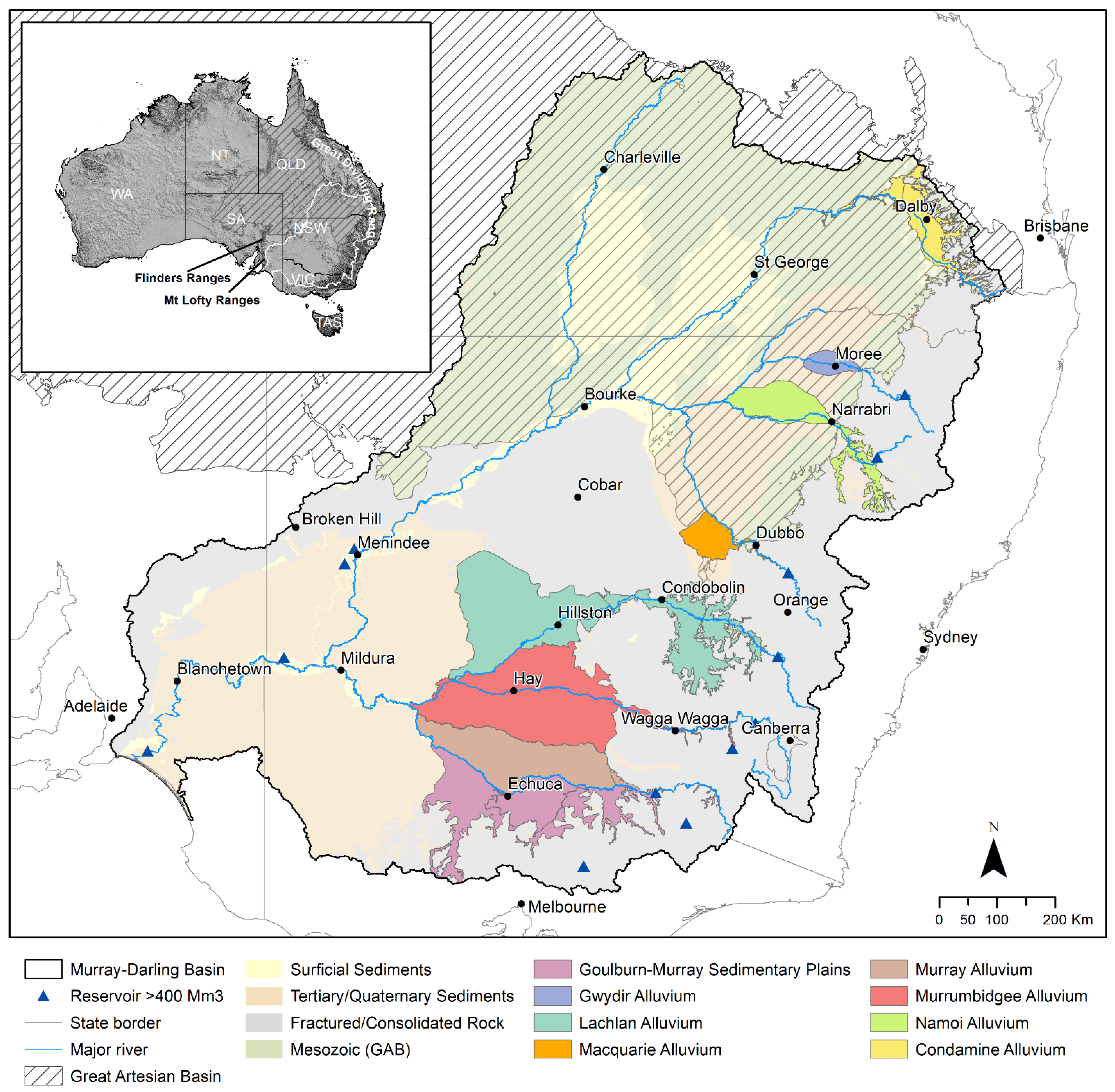
The MDB is an iconic Australian river basin covering more than 1 million km2 and spanning five federated states (New South Wales, Queensland, Victoria, South Australia, and Australian Capital Territory) (Figure 1). It is considered as the “food bowl” of Australia [14,15], with almost all of Australia’s rice and close to 90% of cotton being produced in the basin [15] as well as other major crops, such as cereals, grapes, and horticulture [16]. Irrigated agriculture water use in the MDB accounts for 70% of irrigation agricultural water use in the whole of Australia, which is used to support around 1.5 million hectares of irrigated crops and pastures [17,18]. As shown in Figure 1, most of the irrigated agriculture concentrates in the main alluvial aquifers of the basin, which account for nearly 80% of the metered groundwater use in certain years. The MDB also meets water needs for nearly 2 million people and contributes to the water supply of a major city outside the basin (Adelaide, 1.4 million inhabitants) [15]. Groundwater use in the MDB becomes increasingly important during drier periods. For example, the Lachlan region (Figure 1) sources up to 80% of the total water use from groundwater during periods of low surface water availability (compared to an average of 45%) [19], whereas in the northern MDB, a large number of water users rely entirely on groundwater sources [13]. It is anticipated that reliance on groundwater sources as a supply option to meet current and future water needs will increase given the projected changes in future climate [13,17].
Under this context, several authors have analyzed the trends in groundwater levels for individual/local alluvial aquifers in the MDB, considering different time periods, methods, and spatial scales for the analysis. This has resulted in a slightly disaggregated analysis lacking a regional perspective and methodological homogeneity. For example, Kelly et al. [20] showed declining trends in groundwater levels between 1–7 m for the period 1988–2008 using differences in groundwater levels for these years in the Namoi alluvial aquifer (Figure 1), suggesting that a dynamic equilibrium had not been reached. They also showed the occurrence of isolated increasing trends in groundwater levels (<1–2 m) in areas of limited groundwater withdrawals, probably due to leakage from on-farm dams, deep infiltration from irrigated crops, and the removal of trees. McCallum et al. [21] analyzed trends in groundwater levels in the Maules Creek, a tributary of the Namoi River (Figure 1), for two periods (pre-development: 1974–1984 and post-development: 1984–2004), calculating metrics for the pre- and post-development periods. They concluded that groundwater levels showed a long-term decline driven by groundwater abstraction. Clark [10] used unsupervised clustering to identify four patterns/trends in groundwater levels (decreasing, decreasing and even out, constant, increasing over time) in the Namoi alluvial aquifer for the period 1974–2018. Giambastiani and Kelly [22] analyzed the trends in groundwater levels in the Macquarie–Bogan alluvial aquifer for the period 1988–2008, and using the same approach as [20], identified declines between 0–2 m reaching up to 13 m. These authors also identified localized sectors showing rising trends in groundwater levels associated with increased deep percolation rates related to irrigation deep drainage. Le Brocque et al. [23] used the Mann–Kendall and Sen’s slope methods to detect persistent groundwater level decline trends (average 0.06 m/y) in the Condamine alluvial aquifer for the period 1989–2015 despite a number of targeted policy interventions. Burkett and Kelly [24] analyzed the groundwater level trend in the Lachlan aquifer for the period 1988–2008 using the same approach as [22], identifying specific hotspots with groundwater level declines between 10 and 30 m. They also identified areas with no substantial declines for the period analyzed, thus highlighting the importance of spatial patterns and the occurrence of zones of high groundwater withdrawals. Finally, recently the Australian Bureau of Meteorology [6] has developed a continental scale tool to visualize information on 5-, 10- and 20-year groundwater level trends (from year 2000 onwards) from upper aquifers, which can be associated with the alluvial aquifers shown in Figure 1. These trends are calculated using a linear regression fitting over the annual groundwater level recovery peak [6].
In this work, we present a methodologically consistent and regional trend analysis of groundwater levels in the main alluvial aquifers of the MDB using a consistent 40-year time window contained between years 1971–2021. The trend analysis is based on robust and widely-applied statistical techniques [12,25], and was performed on 910 observation bores out of nearly 1200 available for monitoring in the MDB [17]. For spatial consistency, we performed the trend analysis for each of the so-called sustainable diversion limit areas (groundwater resource units) defined in the Basin Plan 2012. The term “sustainable diversion limit (SDL)” is used in Australia to define a geographical area/groundwater source within the MDB associated with a long-term annual average limit on how much water can be used for consumptive purposes. It is employed for managing groundwater resources as defined by the Basin Plan. The SDL areas are analogous to ‘groundwater management units’ used in groundwater management plans in other countries [26,27,28]. The contribution of our work lies in presenting a temporally and spatially consistent trend analysis for the main alluvial aquifers of the MDB in order to obtain a regional perspective of the status of the key groundwater resources of the basin. We also attempt to disentangle regional trend patterns by attributing potential drivers to these regionalized trends in groundwater levels.
The remainder of the article is organized as follows. Section 2 describes the study area highlighting the main alluvial aquifers, data selection criteria, and statistical methods employed. Section 3 presents the main results of the analysis. Section 4 provides a discussion of these results, and we offer concluding remarks in Section 5.
2. Materials and Methods
2.1. Study Region
The MDB is Australia’s largest and most important river system, covering 1,060,000 km2 or roughly one seventh of the Australian continent (Figure 1). The MDB is home to about 2 million people and provides the potable water supply to another 1 million outside the basin. The MDB provides the water for 75% of Australia’s irrigation industry and this underpins the basin providing 34% of Australia’s agricultural output. The climate in the MDB varies from sub-tropical in the north, Mediterranean in the south, alpine in the south-east, and semi-arid in the west. The mean annual rainfall, areal potential evapotranspiration, and runoff averaged over the entire MDB are 457, 1443, and 27 mm, respectively. There is a clear east–west rainfall gradient, where rainfall is highest in the south-east (mean annual rainfall of more than 1500 mm) and along the eastern perimeter, and lowest in the west (less than 300 mm) [29].
Groundwater systems across the MDB can be subdivided into three major provinces [13,29,30,31,32] (Figure 1): (i) fractured rock aquifers contained in the Mt Lofty/Flinders Ranges in South Australia, and in the Great Dividing Range, which forms the eastern and south-eastern margins of the Basin; (ii) alluvial aquifers contained in major river valley deposits, where river leakage and flood events are major sources of recharge and most of the irrigated agriculture in the MDB is located; and (iii) tertiary limestone of the western Murray Basin where groundwater is primarily saline with areas of good quality groundwater. Stewardson et al. [30] acknowledge a fourth province associated with the Great Artesian Basin (GAB) sediments, located in the northern MDB sub-basin. Most of this province in the MDB consists of recharging/intake beds or confining sediments (at the surface) to the underlying main (deeper and confined) GAB aquifers. This province is not included in this analysis as the GAB aquifers show limited connection and flow exchanges with surface alluvial aquifers [30].
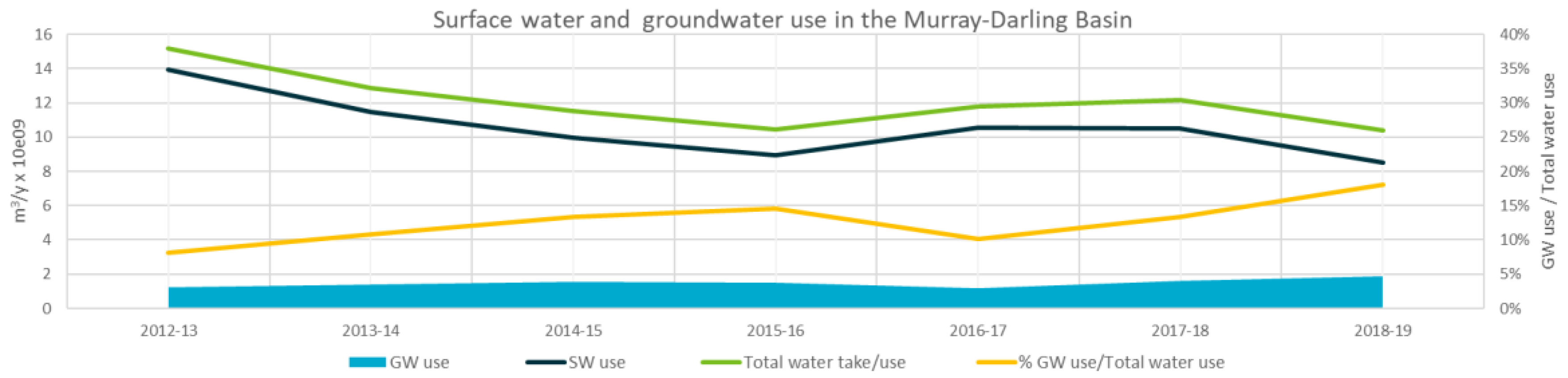
Figure 2 shows the water use across the MDB for the period 2012-13 to 2018-19 as reported from the Transition Water Take Reports (2012-13 to 2018-19) [31]. This data covers the entire Basin use and is considered of high reliability in terms of quality assurance compared to previous reporting (2001-02 to 2011-12), thus providing valuable insights on total groundwater use. Average groundwater use in the MDB is 1.482 × 10⁹ m3/y and represents about 13% of the total water use reported in the MDB, ranging between 8% and 18% for the period analyzed. Proportional contributions from groundwater to the total available water resources are complementary to surface water resources, and therefore they increase when surface water availability decreases.
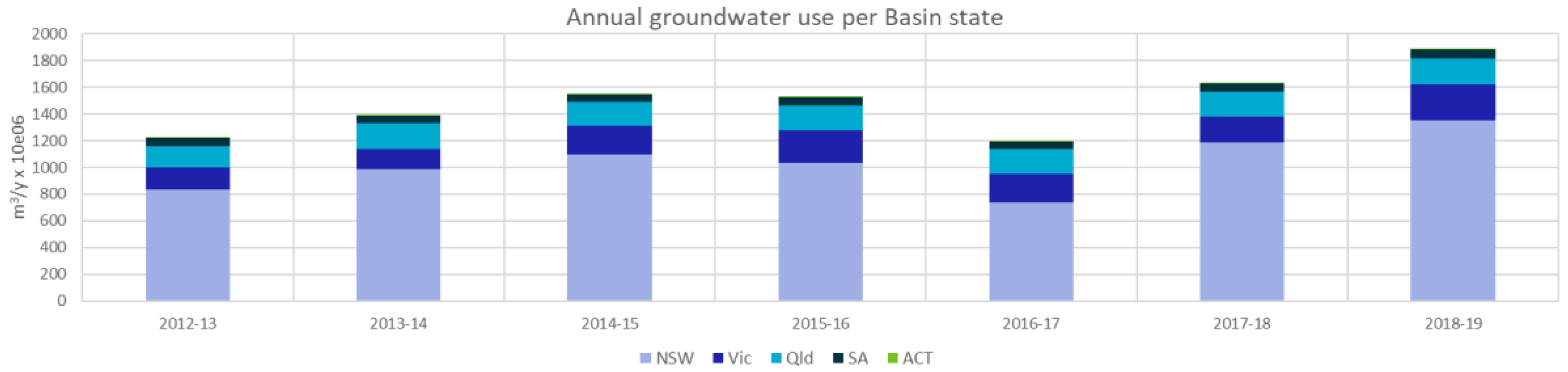
The Murray–Darling Basin Authority (2020) highlights that 92% of the total groundwater annual actual take (use) was metered for the year 2018-19, whereas 100% of the groundwater take under basic rights (domestic and stock) is unmetered. This suggests that recent statistics on groundwater use are more reliable compared to earlier estimates, notwithstanding the lack of metering for groundwater take under basic rights. The latter has been estimated at about 2.33 × 10⁸ m3/y for the period 2015-16/2018-19. At the state level for the period 2012-13 to 2018-19, New South Wales (69%), Queensland (14%), and Victoria (13%) account for 96% of the total groundwater use reported in the Basin (Figure 3).
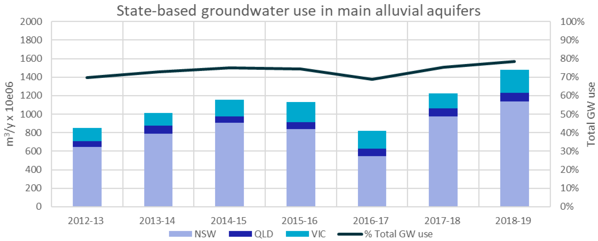
Around 75% of total metered groundwater use is extracted from eight large alluvial systems in these States within the MDB associated with 19 (out of 80) groundwater sustainable diversion limit (SDL) resource units [13]. This study focused analyses of level trends on these eight alluvial systems. Groundwater use from these systems is reported as:
Condamine (Upper Condamine Alluvium—Central GS64a) (This nomenclature corresponds to the 80 groundwater sustainable diversion limits (SDL) resource units reported by the Murray-Darling Basin Authority (https://data.gov.au/data/dataset/66e3efa7-fb5c-4bd7-9478-74adb6277955. Accessed on 15 November 2021). For the period 2012-13 until 2018-19, this alluvial system concentrates on average 43% of the total groundwater use metered by SDL resource units in Queensland, with the most recent estimate bringing this value close to 50%. If groundwater use in the Upper Condamine Basalts (GS65) is also included, the average use amounts to 80% of groundwater use in Queensland.
Gwydir (Upper Gwydir, GS43—Lower Gwydir, GS24). For the period 2012-13 until 2018-19, this alluvial system concentrates on average 4% of the total groundwater use metered by SDL resource units in New South Wales.
Namoi (Upper Namoi, GS47, GS48—Lower Namoi, GS29). For the period 2012-13 until 2018-19, this alluvial system concentrates on average 18% of the total groundwater use metered by SDL resource units in New South Wales.
Macquarie (Upper Macquarie, GS45—Lower Macquarie, GS26). For the period 2012-13 until 2018-19, this alluvial system concentrates on average 5% of the total groundwater use metered by SDL resource units in New South Wales.
Lachlan (Upper Lachlan, GS44—Lower Lachlan, GS25). For the period 2012-13 until 2018-19, this alluvial system concentrates on average 16% of the total groundwater use metered by SDL resource units in New South Wales.
Murrumbidgee (Lower Murrumbidgee Shallow, GS28a—Lower Murrumbidgee Deep, GS28b—Mid-Murrumbidgee, GS31). For the period 2012-13 until 2018-19, this alluvial system concentrates on average 29% of the total groundwater use metered by SDL resource units in New South Wales.
Murray (Lower Murray Shallow, GS27a—Lower Murray Deep, GS27b—Upper Murray, GS46). For the period 2012-13 until 2018-19, this alluvial system concentrates on average 8% of the total groundwater use metered by SDL resource units in New South Wales.
Goulburn–Murray (Shepparton Irrigation Region, GS8a—Sedimentary Plain, GS8c). For the period 2012-13 until 2018-19, this alluvial system concentrates on average 88% of the total groundwater use metered by SDL resource units in Victoria, with the most recent estimate bringing this value to 90%.
At the state level (Figure 4), the Gwydir, Namoi, Macquarie, Lachlan, Murrumbidgee, and Murray alluvial systems in New South Wales represent on average 80% of the groundwater use, with more recent estimates bringing this value to 84% (which is the ratio of water use from these four NSW aquifers in Figure 4 to the total NSW groundwater use in Figure 3). Most of the remaining groundwater use is concentrated in five SDL resource units (Kanmantoo Fold Belt MDB—GS19, Gunnedah–Oxley Basin MDB—GS17, New England Fold Belt MDB—GS37, Western Porous Rock—GS50, and Lachlan Fold Belt MDB—GS20), ranging on average between 8.2 × 10⁶ m3/y and 8.1 × 10⁷ m3/y for the period 2012-13 to 2018-19. In Queensland, the Condamine alluvial system accounts on average for 43% of the groundwater use, with the other three SDL resources units accounting for the remaining 49% of groundwater use (Upper Condamine Basalts—GS65, Queensland Border Rivers Alluvium—GS54, and St. George Alluvium: Condamine–Balonne (deep)—GS61b), ranging between 1.13 × 10⁷ m3/y and 6.73 × 10⁷ m3/y. In Victoria, the Goulburn—Murray alluvial system accounts on average for 88% of the total groundwater use, with SDL GS8b (Goulburn-Murray: Highlands) bringing this figure to 95% for an average consumption of 1.42 × 10⁷ m3/y for the period 2012-13 to 2018-19.
2.2. Datasets
2.2.1. Groundwater Level Data
Bore depth to water table (DTW) data were accessed using the National Groundwater Information System (NGIS) Version 1.7.0 last updated in July 2021 [32]. Bore records with no drilled depth information were excluded. Bores within the selected groundwater SDL resource units were extracted and regolith thickness estimates (thickness of unconsolidated material above bedrock as an indicator of the thickness of alluvial aquifers) were added from a national dataset [33]. Bores drilled deeper than regolith thickness were excluded, as were DTW records deeper than drilled depth or regolith thickness. Bore records from overlapping shallow and deep groundwater SDL resource units were separated based on reported formation thicknesses [11]. These selections were based on the following drilled depths: bores within Goulburn–Murray Sedimentary Plain (GS8c) were >25 m; within Goulburn–Murray Shepparton Irrigation Region (GS8a) were </=25 m; within Lower Murrumbidgee Shallow Alluvium (GS28a) were </=40 m; within Lower Murrumbidgee Deep Alluvium (GS28b) were >40 m; within Lower Murray Shallow Alluvium (GS27a) were </=20 m; and within Lower Murray Deep Alluvium (GS27b) were >20 m.
2.2.2. Data Quality Control and Annual Time Series
Suspicious observations are very common for groundwater level measurements [34]. These can result from simple errors (e.g., a record/management error or failure of a data log) or an unforeseen biophysical and hydrological process (e.g., a flood event, nearby pump testing, or sudden groundwater extraction). Ideally, errors and outliers should be identified, and their associated reasons investigated. Although the latter may provide valuable insights about groundwater dynamics, they still present a challenge for trend analysis. Therefore, outliers were removed for this study, regardless of their mechanism. We have tested a few popular thresholds from a statistical point of view, such as 1.5 times interquartile range (IQR), 99% percentile, and 99.9% (roughly equivalent mean ± 3.1 times standard deviation, SD), and found that mean ± 3.1 SD worked well for our case by successfully removing all obvious errors and outliers and keeping all non-outliers as judged via a visual inspection process.
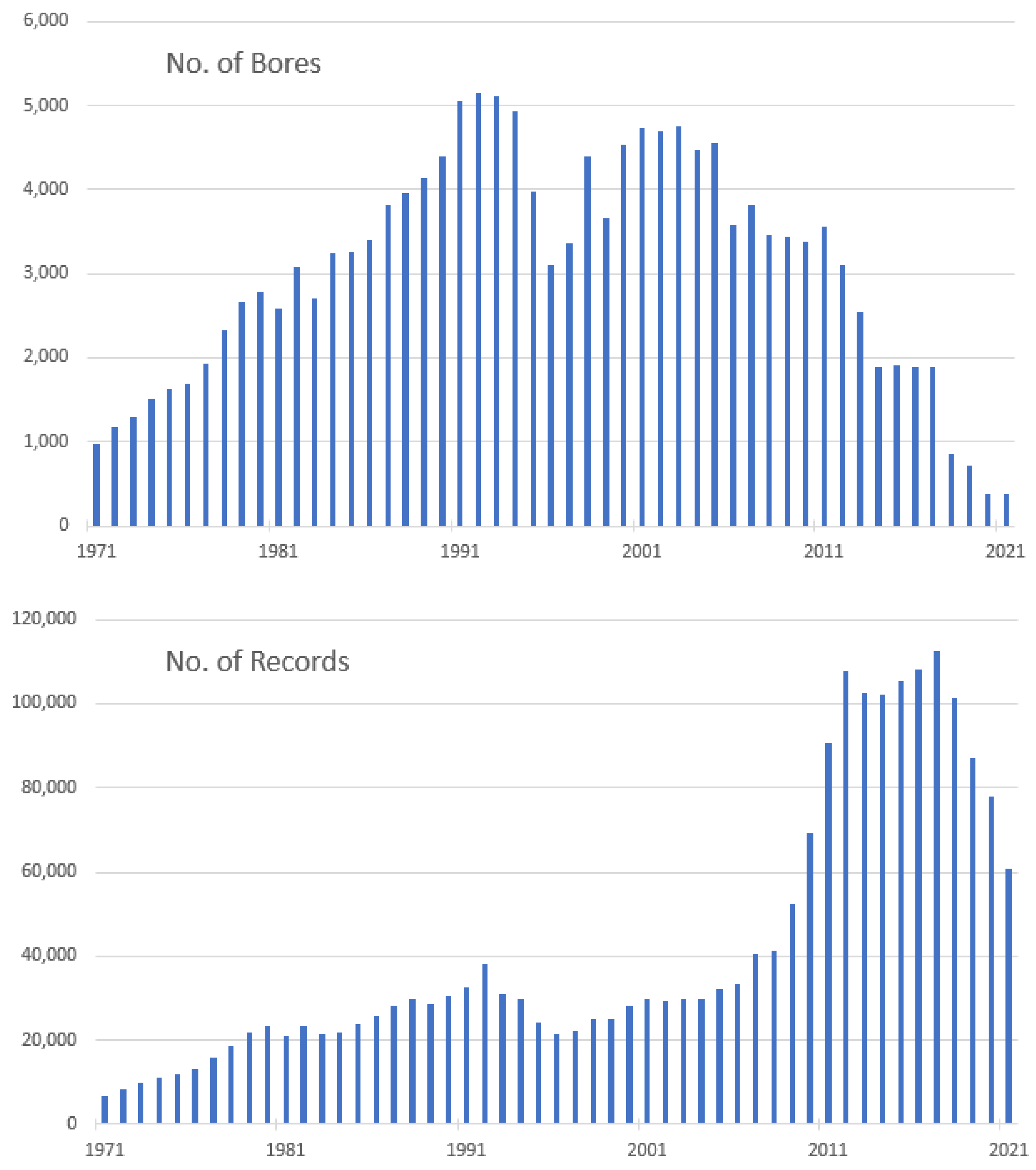
A change in measurement methods, especially from manual field measurement to automatic methods in recent years, can lead to a large variation in the number of data points from year to year at a single bore location. This could result in an unrealistic trend. To avoid this problem, the trend analysis was performed on an annual time scale, i.e., only one DTW value for a single year was used regardless the number of data points in that year (which could be only two manual field measurements or thousands of automatic measurements). To construct the annual DTW time series for trend analysis, at least two observations were required for each year. This assumed the sampling strategy would be designed to detect the highest and lowest groundwater levels in a year so that valid annual mean/minimum/maximum values were derived. Furthermore, at least 40 years of data were required during the 51-year (1971–2021) study period. This restriction reduced the number of actively monitored bores from more than 13,000 to 910 (Figure 5). The number of groundwater level observations significantly increased since 2011, but the number of groundwater bores monitored declined from >4000 in the 2000s to <1000 since 2018 (Figure 5).
2.2.3. Rainfall and PET (SILO)
The SILO Data Drill [35], which provides 0.05° gridded (approximately 5 × 5 km) daily climate variables across Australia, were used in this study to explore trends in annual rainfall and potential evapotranspiration (PET). The dataset was interpolated from station measurements made by the Bureau of Meteorology (BoM). The interpolations of rainfall are based on the smoothing, splining, and kriging techniques described in [35]. The data in the SILO Data Drill are all synthetic; there are no original meteorological station data in the calculated grid fields. PET is calculated with the FAO 56 formula [36].
2.3. Trend Analyses
Three trend detection techniques are used in this study to explore groundwater level trends. Since the variable used is the depth to water table (DTW), an increasing trend means declining groundwater levels, whereas a decreasing trend means rising groundwater levels.
2.3.1. Kendall Test
The nonparametric Kendall’s test is widely used to detect trends in various hydroclimate and water quality variables. It was first adopted by Hirsch et al. [37] and modified from Mann–Kendall’s test [38]. The advantages of this method include (1) it can handle non-normality, censoring, or data reported as values “less than”, missing values, and seasonality; and (2) it has a high asymptotic efficiency [37].
A hypothesis test based on the normalized Kendall’s statistic Z, for a significance level (α), was applied. The test statistic Z, at a particular groundwater bore, was estimated as [37]:
where
where x is the variable (groundwater depth in this case) with a sample size of n, and t is the extent of any given tie, i.e., length of consecutive equal values.
The null hypothesis, Ho, meaning that Z is not statistically significant, i.e., no statistically significant increasing/decreasing trend in groundwater level, is accepted if −Zα/2 < Z < Zα/2, where Zα/2 are the standard normal deviates. Correspondingly, it is accepted that H1 or Z are statistically significant if Z < −Zα/2 or if Z > Zα/2 [39]. As it is possible that some bores have an increasing trend and others decreasing, a two-sided hypothesis was chosen [39]. The same significance level (α = 0.05) as the linear trend analysis was used to detect whether a trend was statistically significant.
In addition to identifying whether a trend exists, it is also very important to establish the magnitude of a trend. The trend magnitude β (beta magnitude) is an estimator developed by Hirsch et al. [37] based on that proposed by Sen [40], and is defined as:
where 1 < i < j < n. The slope estimator β is the median over all possible slope combinations of pairs for the whole data set, X is the time series of groundwater level depth, and n is data length, or the number of years of the dataset, i.e., 1971–2021 = 51 years in this study.
2.3.2. Linear Trend
This basically builds a linear regression between a series of depth to water table measurements and time:
where yt is the groundwater level, t is time, a and b are unknown constants, and et is a randomly distributed error. The values for parameters and are usually estimated by minimizing the sum of the squared errors in the data series, which is why it is also called least-squares regression.
The statistical significance of this linear slope, i.e., whether a = 0, is tested by a t statistic,
which has a t distribution with n-2 degrees of freedom, meaning a p-value can be obtained from this statistic, and n is the sample size. The parameters se and sx are computed as follows:
where e is the residual of the regression e = (∗ t + )—y.
The significance level α = 0.05 (which corresponds to p < 0.025 with a two-sided test) is used in this study to detect whether a linear slope is statistically significant.
2.3.3. Two-Period Comparison and Innovative Trend Analysis (ITA)
The two-period method simply compares mean groundwater levels between two periods of time that do not necessarily need to have equal lengths. To further explore the trends at different quantiles by using the innovative trend analysis (ITA) [41,42], equal lengths of periods are required. If the mean value for the second half period is higher than the first half, a rising trend is detected, and vice versa. The statistical significance can be tested to determine whether the values are substantially different:
where and are the mean values for the first and second half, respectively. The and are standard deviations of two periods. The statistic t has a t-distribution with n-1 degrees of freedom. The trend magnitude, S-slope, is estimated based on the ITA method [41,42]:
The advantage of extending a simple two-period method into the ITA method is that it can show different trend directions and magnitudes for different quantiles of groundwater levels. For example, it can show where trends for lower values differ in both direction and magnitude from trends at higher values. This can provide insights into the likely mechanisms driving observed trends.
3. Results
3.1. Groundwater Level Trend Significance and Magnitudes
There is clearly an overall increasing trend in DTW for the MDB alluvial aquifers during the last 50 years (1971–2021), regardless of the groundwater level statistic (mean, minimum, and maximum annual values) or the trend detection method used in the analysis (non-parametric Kendall test, linear regression, and two-period comparison) (Table 1).
About 90–95% of groundwater bores show an increasing trend in depths, of which 84–87% are statistically significant at α = 0.05. In contrast, only 7–9% of groundwater bores show a decreasing trend in depths, and 4–5% are statistically significant (Table 1).
In terms of trend magnitudes, these range from −0.25 to about +1.00 m/year across all three annual groundwater level statistics (mean, minimum, and maximum annual values) and the three analysis techniques for the 50-year period assessed (1971–2021). The median and mean values for the 910 groundwater bores are 0.09 and 0.11–0.13 m/year, respectively (Table 2).
While the maximum trend magnitude can be as high as +1.0 m/year, the 95th percentile is about 0.3–0.4 m/year (Table 2). The 5–10% negative trend magnitudes are consistent with the trend significance results (Table 2).
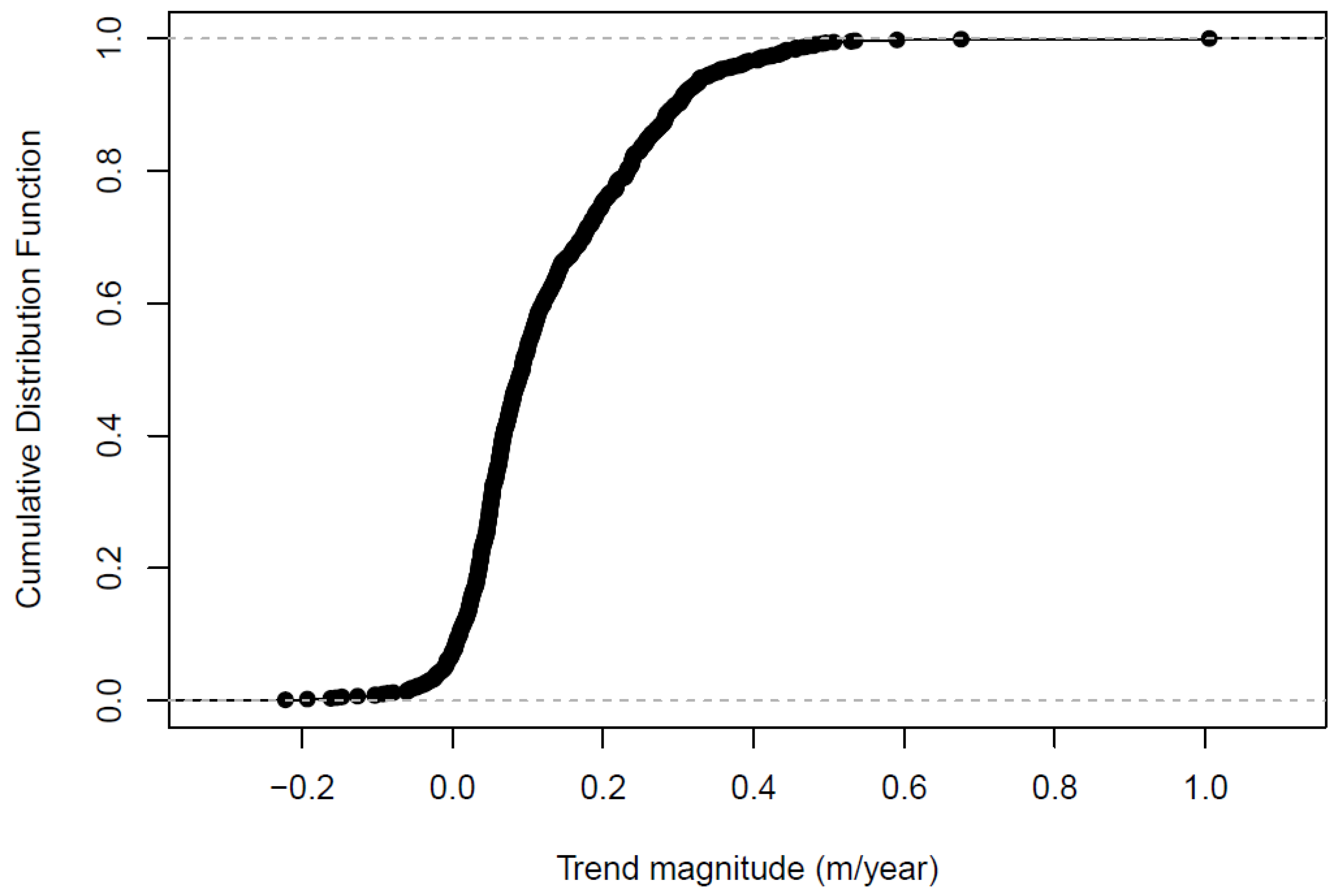
The cumulative distribution function (cdf) of trend magnitude for the annual mean groundwater level from the beta magnitude (β) (Figure 6) shows the detailed distribution of trend magnitudes. The other statistics and methods have a very similar distribution. It is also interesting to note that the maximum trend magnitudes from S-slope for the two-period comparison method are relatively smaller (0.82–0.83 m/year) than the other two methods (0.98–1.01 m/year), whereas their 75th percentile values are almost the same (Table 2). Other differences are mainly seen at the higher end (P90 or above), which also leads to differences in mean trend magnitudes, even if they have similar median values.
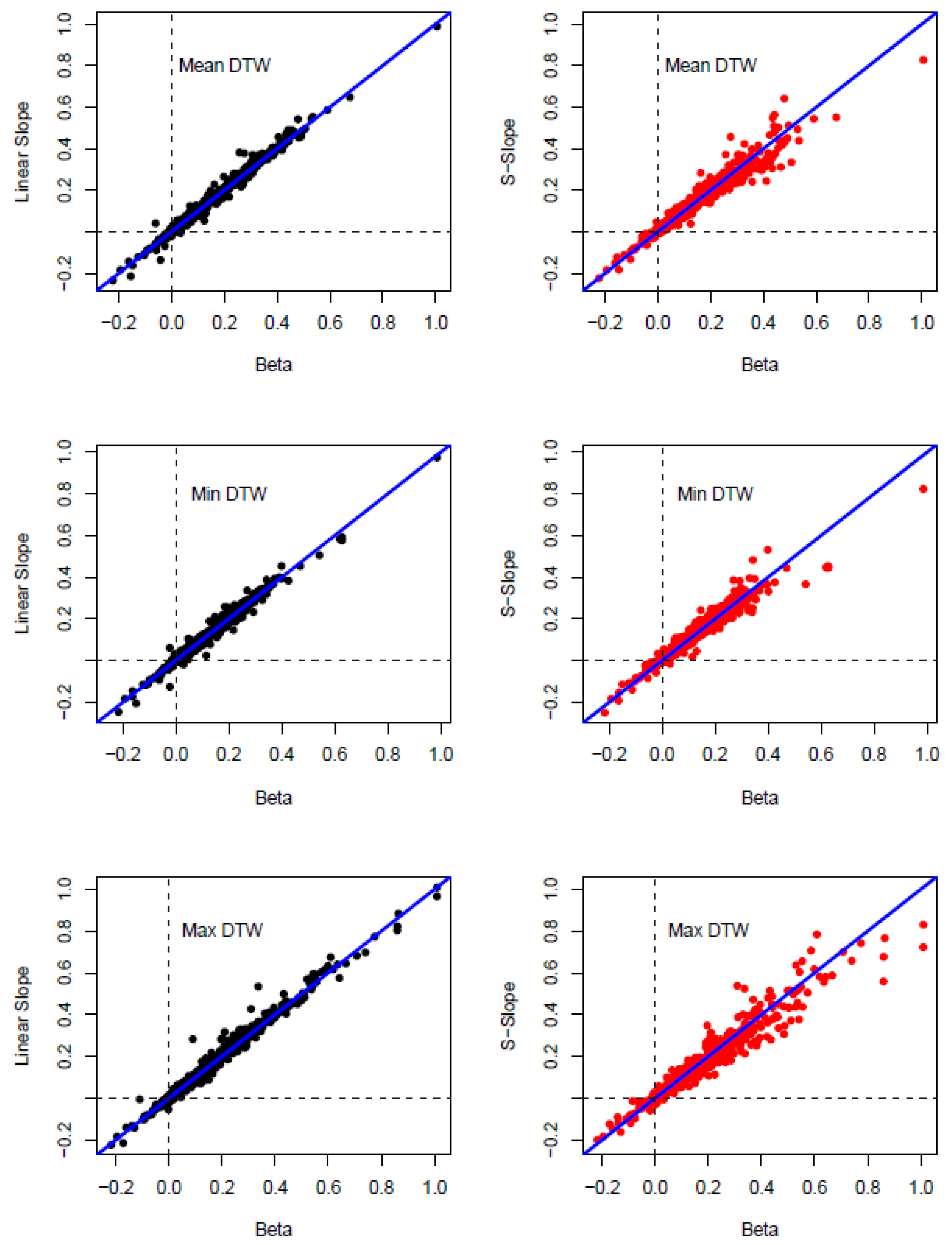
Overall, the three trend methods show consistent results for both trend significance (Table 3) and trend magnitude (Figure 7): (a) About 95% of groundwater bores show exactly the same trend significance, i.e., the diagonal values in Table 3. In contrast, there are no bores that show opposing statistically significant trends, e.g., one method indicates an increasing trend, but a second method shows a decreasing trend. This is reflected by the zero values shown in anti-diagonal (Table 3). (b) The linear regression method shows greater consistency with both the Kendall method (95.8%) and the two-period comparison (95.5%) than the Kendall method with the two-period comparison (94.3%). (c) Table 3 describes annual mean groundwater levels, but the general conclusion also applies to annual maximum and minimum groundwater levels in the dataset. (d) The trend magnitudes from the three methods are generally consistent (Figure 7), especially between the beta (β) and linear regression slope methods. The two-period S-slope, however, shows relatively smaller trend magnitudes and slightly larger inconsistencies when compared with the beta slope method. (e) A few groundwater bores show opposing trend directions, although these are not statistically significant (ca. 1% of total number of bores analyzed); similarly, there were few instances where there was a large difference in trend magnitudes (same trend sign but different magnitudes) (Figure 7).
3.2. Groundwater Level Trend for Different Statistics
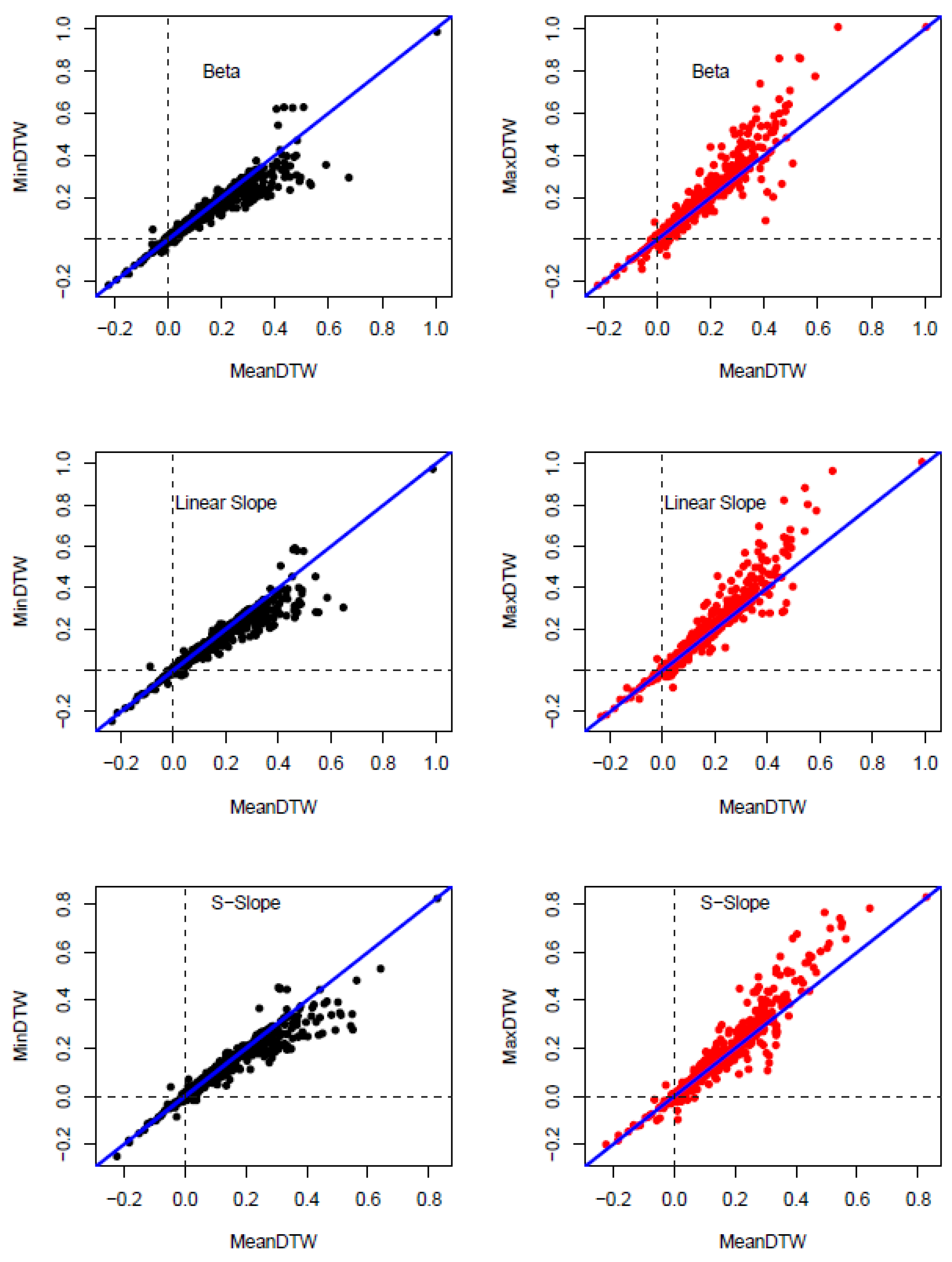
Figure 8 shows the trend magnitude comparisons for the three annual groundwater statistics, and clearly shows that MinDTW has a smaller trend magnitude than MeanDTW (more dots below the 1:1 line) and MaxDTW has a larger trend magnitude than MeanDTW (more dots above the 1:1 line). This was consistent for all three analysis methods.
It is interesting to note the differences are bigger for the larger trend magnitudes and smaller for the minor or negative trend magnitudes, i.e., the points are almost on the 1:1 line for the smaller trend magnitudes and depart from 1:1 line for the larger trend magnitudes (Figure 8). The position of this departure can be associated with underlying physical processes. Smaller trend magnitudes are likely to result from rainfall-driven groundwater recharge; consequently, annual mean/minimum/maximum groundwater levels exhibit similar trend magnitudes. Larger trend magnitudes are generally the result of groundwater extraction combined with rainfall-driven recharge; therefore, annual minimum groundwater levels demonstrate smaller trend magnitudes due to rainfall-recharge, but larger trend magnitudes for annual maximum levels due to groundwater extraction (Figure 9).
3.3. Spatial Distributions of Groundwater Level Trend Significance and Magnitudes
Figure 10 shows the spatial distribution of trend significance and magnitudes for annual mean groundwater levels determined by the Kendall test. The overall statistically significant increasing DTW trend can be clearly observed across all areas (Figure 10a). Most groundwater bores with declining groundwater levels (increasing DTW) lost 0.0–0.2 or 0.2–0.3 m/year (Figure 10b). It can be concluded that there was a consistent trend towards long-term groundwater level declines of around 0.2 m/year on average across all aquifers assessed in this study, with some areas showing steeper declines of up to 1 m/year. There were far fewer bores where water levels increased (decreased DTW) (Figure 10c,e). These trends were statistically significant, though the magnitudes for these bores were generally in the lower −0.2–0 m/year range (Figure 10d,f). Clusters of bores that showed higher water level declines were evident in all aquifers (Figure 10b), indicating intensive extraction and the potential development of localized cones of depression.
Bores in the Goulburn–Murray Sedimentary Plain aquifer displayed a decreasing level trend with average magnitudes ranging from 0.1 to 0.59 m/year. The overlying Shepparton Irrigation Region, however, showed mixed trends with some bore levels increasing and some decreasing with trend magnitudes ranging from −0.15 to +0.21 m/year (Table 4). This was expected due to known issues with groundwater salinity; as a consequence, active management through groundwater extraction is being used to control water table depths and reduce the risk of soil salinization in the Shepparton Irrigation Region [11].
The deep bores in the Lower Murrumbidgee aquifer showed larger trend magnitudes than those in the shallow alluvium (median, 0.17 vs. 0.04 m/year; mean, 0.18 vs. 0.03 m/year, respectively), as well as a larger range (−0.22 to +0.50 vs. −0.06 to +0.09 m/year, respectively) (Table 4). Comparing trend magnitudes between shallow and deep aquifers was limited for two main reasons: firstly, there were insufficient data from both shallow and deep aquifers; and secondly, the degree of interaction was expected to be variable in both space and time.
3.4. Attributions of Groundwater Trend
Variations and trends in groundwater levels are generally dominated by two main processes: natural recharge and discharge, and groundwater extraction [43]. For upper alluvial aquifers with good hydrological connection to the surface, rainfall driven recharge, either directly or through seepage from water bodies, results in a groundwater level increase, whereas groundwater discharge to waterbodies, seepage into lower aquifers, and evapotranspiration through deep rooted plants results in decreasing groundwater levels under conditions of non-equilibrium. Natural groundwater discharge or loss processes will generally occur more gradually over time and more diffuse in space. Groundwater pumping, especially intense applications (e.g., for agricultural irrigation or mine dewatering), can cause more rapid and localized water table declines compared to natural discharge processes. In this study, we compared groundwater level trends and magnitudes with climate data and a measure of groundwater development (a proxy for pumping intensity) over time to associate observed trends with specific processes.
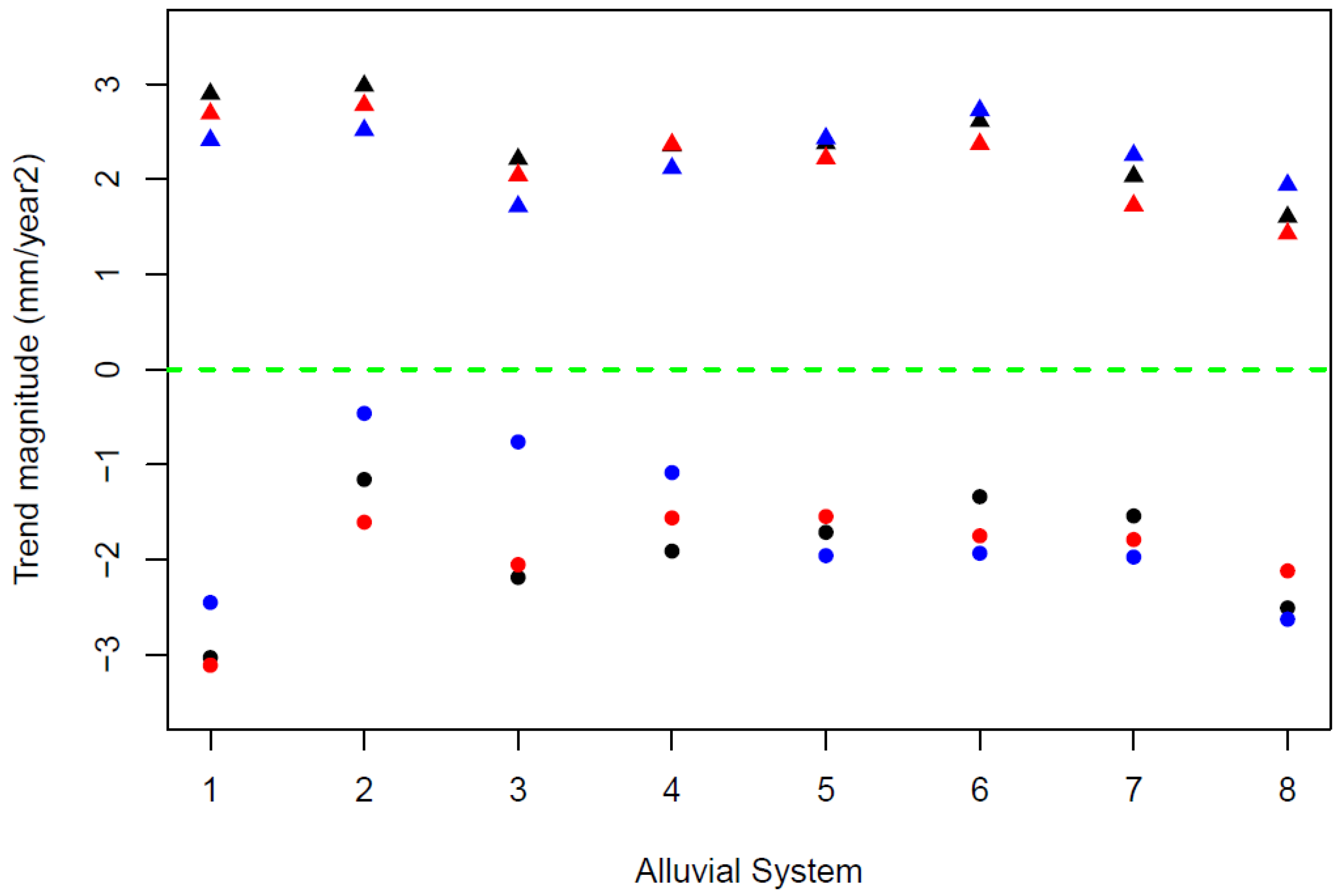
Figure 11 shows the trend magnitude (mm/year2) of annual rainfall and PET for the eight alluvial aquifers studied in the MDB for the period 1971–2021. Across all aquifers, regardless of the trend analysis method used, long-term reductions in average annual rainfall of between 0.5 and 3.2 mm/year are evident. Similarly, across all aquifers and methods, long-term increases in average annual PET of 1.5 to 3 mm/year are seen. These trends in rainfall and PET are consistent with results in the literature [44], partly due to the Millennium Drought during 1997–2009 [45]. These results suggest that the general trend for long-term groundwater level decline seen across all alluvial aquifers (Figure 10, Table 4) can, to some degree, be attributed to decreased rainfall-recharge as a result of lower rainfall and higher PET.
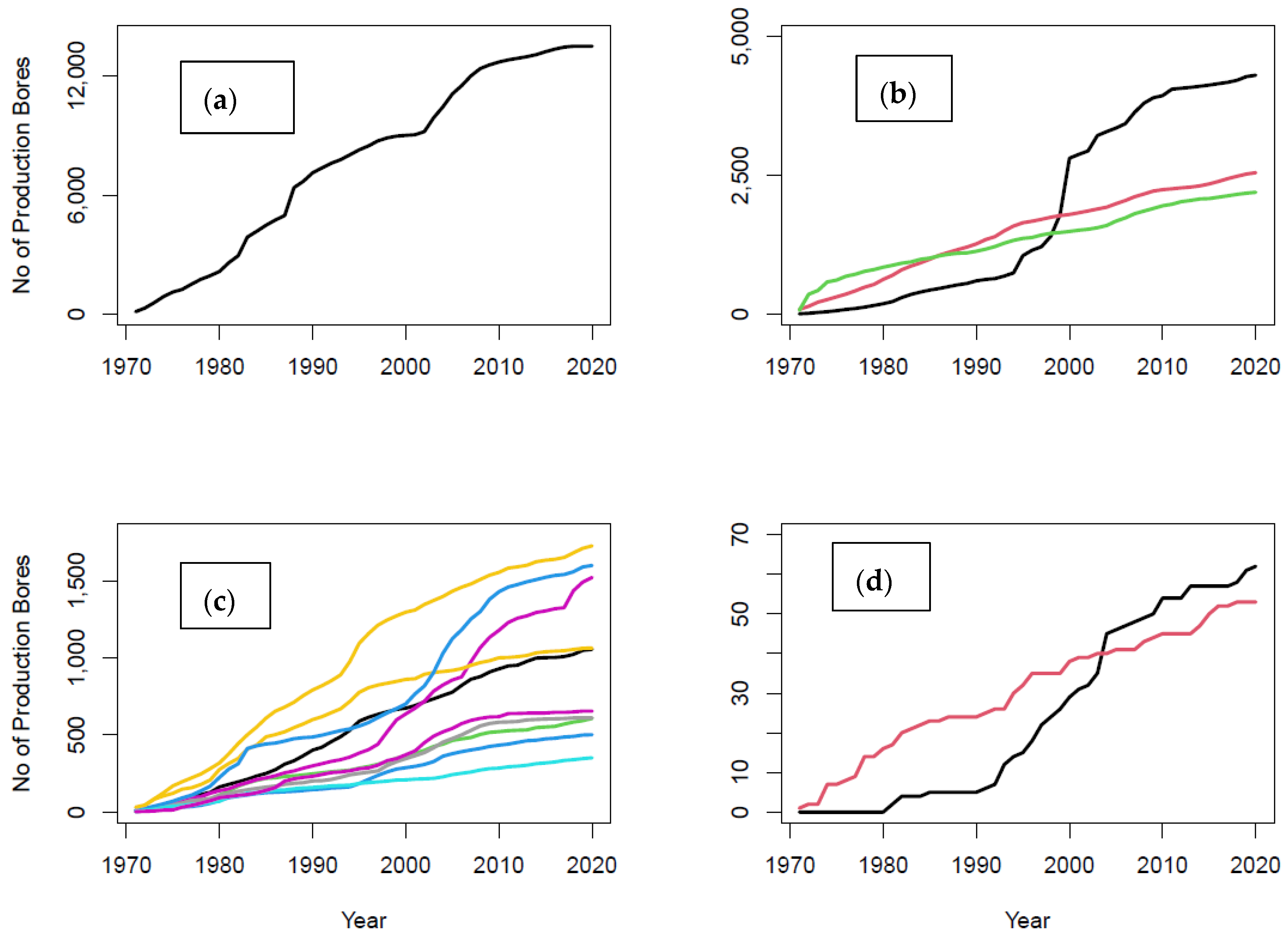
Long-term time series of groundwater extraction volumes were not available for the study areas in the MDB, so extraction rates could not be directly compared with our long-term groundwater level trend analyses. The cumulative number of new bores drilled in each aquifer since the 1970s was calculated and used as a proxy for extraction over time and an indicator of the rate of development of groundwater resources. The number of production bores has increased in the last 50 years across all studied alluvial aquifers, with a marked increase in the 2000s coinciding with the Millennium Drought when surface water became very scarce (Figure 12).
The total number of production bores varies from <100 in some SDL areas (Figure 12d) to >12,000 in others (Figure 12a). The rate of development, as indicated by the cumulative number of bores drilled over time, also varies across these areas. Notable increases are seen during the mid-late 1990s and into the mid-2000s for several areas, whereas other areas show a steady increase over time.
Despite the limitation in groundwater use data, we used the available data for the period 2012–2019 to correlate mean DTW trend values and mean groundwater use reported at the SDL level (Table 4). From this analysis, we obtained a moderate correlation (r = 0.68, p-value = 0.008) between the increasing trend in mean DTW and an increase in groundwater use at the SDL scale.
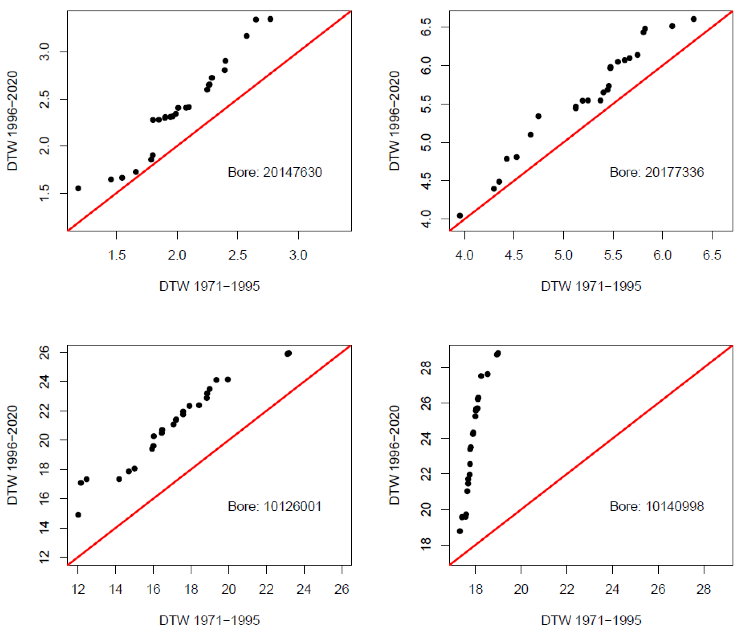
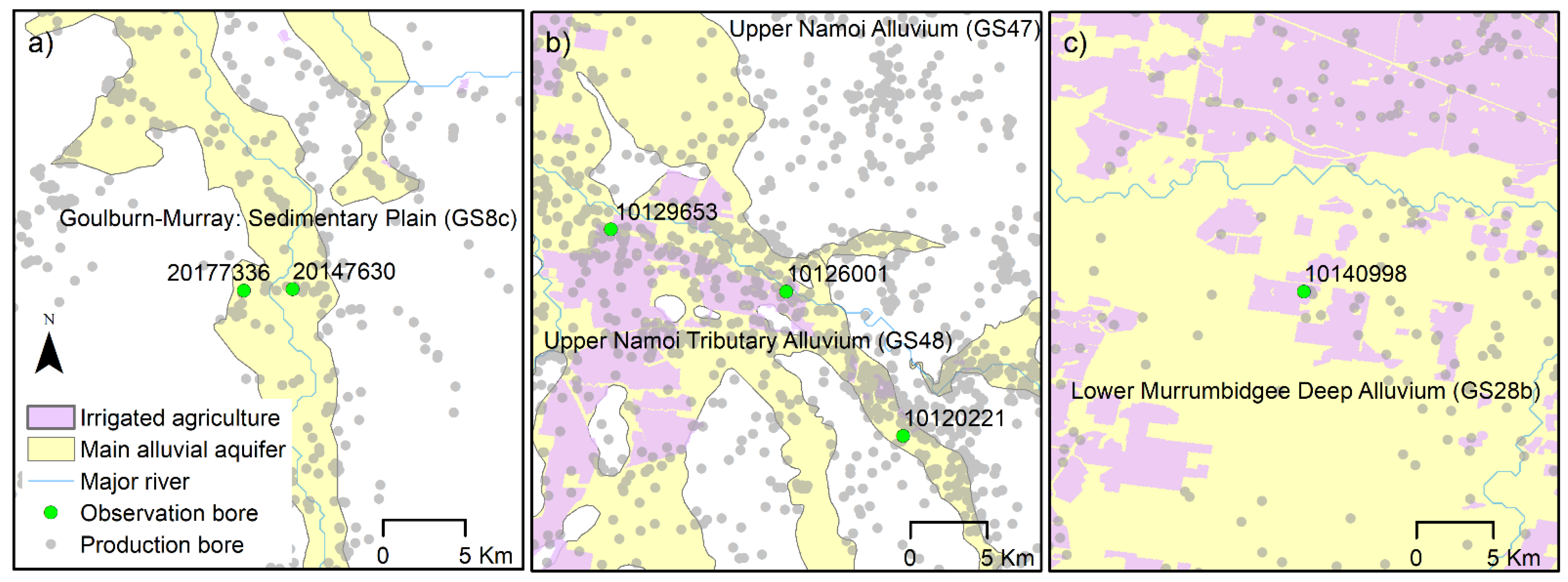
Innovative trend analysis (ITA) results can also be used to explore attributions for groundwater level trends. Figure 13 shows examples of ITA outcomes for four bores, which were chosen because they represent different mechanisms for groundwater level fluctuations. Bores 20147630 and 20177336 are located within 5 km of each other in the upper part of the Goulburn–Murray Sedimentary Plain (GS8c) and are not near areas of irrigated agriculture (Figure 14a). These bores seem to be recharge-dominated as their trend magnitudes for groundwater level fluctuation are relative minor and show similar departures from the 1:1 line across the data distribution. The differences in groundwater levels at bore 10126001, which is in the Upper Namoi Tributary Alluvium (GS48) and within an irrigation area (Figure 14b), probably result from a combination of recharge and groundwater extraction. The increase in DTW between time periods and the departures are about parallel to the 1:1 line, implying a decline in water levels of around 2 m across the data distribution. Bore 10140998 in the Lower Murrumbidgee Deep Alluvium (GS28b) is also within an irrigation area (Figure 14c) and shows a clearly different pattern, where lower values show little difference and higher values are markedly different (>8 m deeper in the later period), which is indicative of much higher extraction rates in the later period (Figure 13).
4. Discussion
4.1. Trend Method Selection
Three popular trend methods were used in this study to detect trends in groundwater levels in eight main alluvial aquifers of the MDB. Overall, results from all three methods were similar. A general methodological recommendation would be that all three methods should be used for trend analysis. These methods showed consistent results for most groundwater bores, and a multi-model analysis enhanced our confidence in the trend results. Potential differences among methods should be further investigated to uncover potential unforeseen biophysical and hydrological process, such as a flood event, pump testing, sudden groundwater extraction, or a new mining site.
However, attention should be paid to those bores where different analysis methods showed different trend signs and magnitudes (Table 2 and Table 3). For example, the Kendall test indicated an increasing trend in the groundwater level at bore 42230669A (Figure 15) due to the fact that the groundwater level was deeper before 2007. In contrast, the linear regression method indicated a decreasing trend due to four shallow observations after 2011 (Figure 15), which indicates a substantial recovery in groundwater level. Further investigation should be carried out to explore the physical processes of groundwater dynamics at this bore after 2007 (especially after 2011).
4.2. Comparison with Existing Results
This study is the first comprehensive trend analysis for all major alluvial aquifers in the MDB, and an overall increasing DTW is identified. This is consistent with some local scale studies in the literature, some of which might be reported as a decreasing trend if the absolute level (such as the Australian Height Datum or AHD) is used. In either case, the groundwater levels across alluvial aquifers of the MDB appear to be growing deeper with time. For example, Welsh et al. [46] showed declining groundwater level trends for both shallow and deeper aquifers in the Lower Gwydir (GS24) and Lower Namoi (GS29) SDLs, with some recovery from 1996 to 2001 due to wetter seasons resulting in reduced groundwater extraction and increased recharge. NSW DPI [47] showed a declining trend in groundwater levels in the Lower Gwydir SDL concentrated around the central area, with more substantial declines west of Moree. NSW DPI [48] also showed a long-term declining trend in groundwater levels between the 1970s (pre-development) and 2015/2016, reaching values greater than 10 m north of Wee Waa.
In the Upper Macquarie alluvial aquifer (GS45), [49] suggested a dynamic equilibrium has been reached around 10 m below pre-development groundwater levels (1970s), which showed a marked declining trend between 1972 and 1992. A less clear situation is depicted for the lower Macquarie alluvial aquifer (GS26), where [49] suggested marked seasonal fluctuations with overall declining trends of 5 m in the last 15 years, as well as groundwater levels fluctuating around a new dynamic equilibrium. Both [24,50] identified specific hot-spots of localized declining trends in groundwater levels in the Lachlan alluvial aquifer, highlighting evidence of a river-aquifer connection and groundwater level responses to episodic recharge from flood events.
4.3. Regional vs. Individual Groundwater Bore Trend
Although an overall increasing trend was identified for the DTW, there was always one bore showing the opposite trend at almost every SDL (Table 4) due to the complicated hydrogeological setting and physical processes. This implies that variation in the spatial groundwater level may be much more intricate than the monitoring network can identify [50]. Therefore, the trend and variation in groundwater level at any individual bore may be much larger/smaller, and even in a different direction, than the regional-scale trend. That is to say, the trend presented is highly subject to the location and depth of individual monitoring bores [51] and the conditions driving local recharge/discharge processes. For example, groundwater levels within the shallow aquifer of the Lower Murrumbidgee (GS28a) require careful interpretation because the aquifer may vary considerably in depth and thickness, as well as its hydraulic properties.
There was a slightly declining DTW trend in the west of the Lower Murray Deep SDL (GS27b) since the mid-1990s due to regional pumping effects [11,52], whereas a rising trend in DTW was reported by [52] towards the eastern section. This is because the groundwater extraction is low in this area due to high salinity groundwater.
4.4. Shallow vs. Deep Aquifers
Groundwater levels in the Lower Murrumbidgee Deep Alluvium (GS28b) compared with those in the Lower Murrumbidgee Shallow Alluvium (GS28a) showed a larger declining trend magnitude (median of 0.04 compared to 0.17 m/year, respectively) and a larger range (0.03 compared to 0.28 m/year, respectively) (Table 4). Results reported elsewhere [51] indicated a mixed pattern of both increasing and decreasing trends in groundwater levels in the shallow alluvium and substantial long-term declines in groundwater levels (up to 12 m) in the deep alluvium. The reasons for these differences are complicated by complex hydrogeology and direct comparison of results are confounded by the different bores and study periods assessed, and therefore, needs further investigation to reach a conclusion.
These alluvial formations are probably not vertically distinct units, either geologically or hydraulically. Different bore completion depths including nested piezometers (i.e., pipes completed at different depths within the same bore hole) may not necessarily align with distinct hydrostratigraphic units, especially in areas with variable vertical hydraulic connections and interactions between shallow and deep groundwater SDL resource units.
4.5. Data Quality and Uncertainty
Data quality is always the core of trend analysis: (a) The groundwater level observations are generally acceptable, but obvious errors and outliers exist. A simple method was used to remove potential errors, but this cannot guarantee an error-free analysis. (b) At least two observations were required to produce an annual mean groundwater level. This is based on a sampling strategy that could capture the highest and lowest groundwater levels. This assumption is not always valid and needs further investigation to be verified. (c) SILO rainfall and PET data have been widely used for various engineering and scientific applications. However, a recent study implied this data could also generate larger than expected uncertainty, especially in the regions with limited weather stations, mountain regions where different algorithms were used to deal with elevation, and coastal regions where an extrapolation was needed to obtain coastal rainfall from inland observations [53]. (d) The biggest challenge for the attribution of groundwater level trends is the nonexistence of reliable long-term groundwater extraction data.
4.6. Quantitative Attributions of Groundwater Level Trend
Variations of groundwater levels are generally dominated by two main processes: natural recharge and discharge, and groundwater extraction. In this study we found that the DTW trend was consistent with a decline in annual rainfall, an increasing trend in potential evapotranspiration, as well as growth in the number of production bores in the MDB. However, we have not built a model to identify the important factors and attribute their respective contribution to the change in groundwater table in a quantitative way [43]. This would require a reliable regional-scale database of groundwater extractions for a longer period than is currently available (2012–2019). Despite this limitation, we were able to observe a moderate positive correlation (r = 0.68, p-value = 0.008) between groundwater use and an increasing trend in DTW for the period 2012–2019, suggesting that groundwater use has contributed to the recent increasing trend in DTW. The complexity of groundwater dynamics at the local scale hinders the attribution process from bore to bore, or even between zones within an alluvial aquifer. For example, two nearby groundwater bores can show opposite trends in groundwater level for totally different reasons (Figure 10).
5. Conclusions
Groundwater is the largest reservoir of liquid fresh water on Earth and is an important source for human consumption, economic development, and provision of ecosystem services. Groundwater levels represent the aggregation of different hydrological processes acting at multiple spatial and temporal scales within aquifer systems. Understanding groundwater level trends is therefore essential to quantifying available groundwater resources and to better manage water resources. Three trend analysis methods were used in this work to detect long-term trends in annual mean/minimum/maximum depth to water table (DTW) at 910 bores in eight main alluvial systems in the Murray–Darling Basin (MDB) Australia, which account for 75% of the groundwater use of the basin. The main conclusions of this work can be summarized as follows:
- The three analysis methods employed showed similar statistical significances and magnitudes, but differences were detected. A general conclusion would be that all three methods should be used for trend analysis since consistent results will enhance confidence in the measured trends, and any differences should be further investigated to uncover potential unforeseen hydrological processes acting on different temporal and/or spatial scales;
- Innovative trend analysis (ITA), which is less popular than the Kendall test and linear regression, could also be used to explore the attributions for the groundwater level trends observed;
- The annual minimum DTW had a smaller trend magnitude than annual mean DTW, and the annual maximum DTW had a larger trend magnitude than mean DTW;
- An overall increasing trend in DTW was identified across all alluvial aquifers, attributable to changes in recharge from rainfall and groundwater extraction;
- Irrigation is responsible for some decreasing trends in DTW, i.e., an increase in groundwater level most likely due to localized recharge processes in shallow aquifers from irrigation;
- There are a few uncertainties associated with the results of this study, which include, but are not limited to, the limited available data on metered groundwater use, the potential errors and outliers in groundwater depth observations, and spatial representation/aggregation of gridded climate data;
- The results could be used to target further research and monitoring programs, and inform groundwater resource management decisions in the MDB.
Author Contributions
Conceptualization, G.F., R.R. and D.G.; methodology, G.F., R.R. and D.G.; software, G.F.; formal analysis, G.F., R.R. and D.G.; investigation, G.F., R.R. and D.G.; data curation, D.G.; writing—original draft preparation, G.F., R.R. and D.G.; writing—review and editing, G.F., R.R. and D.G.; funding acquisition, R.R. All authors have read and agreed to the published version of the manuscript.
Funding
This research was funded through the Murray-Darling Water and Environment Research Program (MD-WERP).
Institutional Review Board Statement
Not applicable.
Informed Consent Statement
Not applicable.
Data Availability Statement
Groundwater level data at: http://www.bom.gov.au/water/groundwater/ngis/ (accessed on 16 March 2022). Silo climate data at: https://www.longpaddock.qld.gov.au/silo/ (accessed on 1 June 2022).
Acknowledgments
We would like to thank Owen Russell and Tariq Rana from MDBA and the two anonymous reviewers for their invaluable comments and constructive suggestions used to improve the quality of the manuscript.
Conflicts of Interest
The authors declare no conflict of interest.
References
- Tillman, F.D.; Leake, S.A. Trends in groundwater levels in wells in the active management areas of Arizona, USA. Hydrogeol. J. 2010, 18, 1515–1524. [Google Scholar] [CrossRef]
- Lasagna, M.; Mancini, S.; De Luca, D.A. Groundwater hydrodynamic behaviours based on water table levels to identify natural and anthropic controlling factors in the Piedmont Plain (Italy). Sci. Total Environ. 2020, 716, 137051. [Google Scholar] [CrossRef]
- Konikow, L.F.; Kendy, E. Groundwater depletion: A global problem. Hydrogeol. J. 2005, 13, 317–320. [Google Scholar] [CrossRef]
- Wada, Y.; Van Beek, L.P.H.; Van Kempen, C.M.; Reckman, J.W.T.M.; Vasak, S.; Bierkens, M.F.P. Global depletion of groundwater resources. Geophys. Res. Lett. 2010, 37, 1–5. [Google Scholar] [CrossRef] [Green Version]
- Famiglietti, J.S. The global groundwater crisis. Nat. Clim. Chang. 2014, 4, 945–948. [Google Scholar] [CrossRef]
- Sharples, J.; Nation, E.; Carrara, E. Groundwater Level Status and Trend Assessment—Method Report; Bureau of Meteorology: Melbourne, Australia, 2021. [Google Scholar]
- Fang, C.; Sun, S.; Jia, S.; Li, Y. Groundwater Level Analysis Using Regional Kendall Test for Trend with Spatial Autocorrelation. Groundwater 2019, 57, 320–328. [Google Scholar] [CrossRef]
- Zeru, G.; Alamirew, T.; Shishaye, H.A.; Olmana, M.; Tadesse, N.; Reading, M.J. Groundwater level trend analysis using the statistical auto-regressive hartt method. Hydrol. Res. Lett. 2020, 14, 17–22. [Google Scholar] [CrossRef] [Green Version]
- Schmid, W.; Pollino, C.; Merrin, L.; Stratford, D. Groundwater Trends in the Brahmani-Baitarni River Basin, India; CSIRO: Canberra, Australia, 2017. [Google Scholar]
- Clark, S.R. Unravelling groundwater time series patterns: Visual analytics-aided deep learning in the Namoi region of Australia. Environ. Model. Softw. 2022, 149, 105295. [Google Scholar] [CrossRef]
- MDBA. Groundwater Report Cards For Sustainable Diversion Limit Resource Units under the Murray-Darling Basin Plan; Murray-Darling Basin Authority: Canberra, Australia, 2020. [Google Scholar]
- Leblanc, M.; Tweed, S.; Ramillien, G.; Tregoning, P.; Frappart, F.; Fakes, A.; Cartwright, I. Ch 10: Groundwater change in the Murray basin from long- term in- situ monitoring and GRACE estimates. In Climate Change Effects on Groundwater Resources Climate Change Effects on Groundwater Resources: A Global Synthesis of Findings and Recommendations; Treidel, H., Martin-Bordes, J.L., Gurdak, J.J., Eds.; Taylor & Francis Group: Boca Raton, FL, USA, 2011; pp. 169–187. [Google Scholar]
- Walker, G.; Barnett, S.; Richardson, S. Developing a Coordinated Groundwater Management Plan for the Interstate Murray-Darling Basin. In Sustainable Groundwater Management: A Comparative Analysis of French and Australian Policies and Implications to Other Countries; Rinaudo, J.M., Holley, C., Barnett, S., Montginoul, M., Eds.; Springer: Berlin/Heidelberg, Germany, 2020; Volume 24, pp. 143–161. ISBN 9783030327668. [Google Scholar]
- Rawluk, A.; Curtis, A.; Sharp, E.; Kelly, B.F.J.; Jakeman, A.J.; Ross, A.; Arshad, M.; Brodie, R.; Pollino, C.A.; Sinclair, D.; et al. Managed aquifer recharge in farming landscapes using large floods: An opportunity to improve outcomes for the Murray-Darling Basin? Australas. J. Environ. Manag. 2013, 20, 34–48. [Google Scholar] [CrossRef]
- Leblanc, M.; Tweed, S.; Van Dijk, A.; Timbal, B. A review of historic and future hydrological changes in the Murray-Darling Basin. Glob. Planet. Chang. 2012, 80–81, 226–246. [Google Scholar] [CrossRef]
- Qureshi, M.E.; Whitten, S.M. Regional impact of climate variability and adaptation options in the southern Murray-Darling Basin, Australia. Water Resour. Econ. 2014, 5, 67–84. [Google Scholar] [CrossRef]
- Gonzalez, D.; Dillon, P.; Page, D.; Vanderzalm, J. The potential for water banking in australia’s murray–darling basin to increase drought resilience. Water 2020, 12, 2936. [Google Scholar] [CrossRef]
- Yu, J.; Fu, G.; Cai, W.; Tim, C. Impacts of precipitation and temperature changes on annual streamflow in the Murray-Darling Basin. Water Int. 2010, 35, 313–323. [Google Scholar] [CrossRef]
- CSIRO. Water Availability in the Murray-Darling Basin; CSIRO: Canberra, Australia, 2008. [Google Scholar]
- Kelly, B.F.J.; Timms, W.A.; Andersen, M.S.; McCallum, A.M.; Blakers, R.S.; Smith, R.; Rau, G.C.; Badenhop, A.; Ludowici, K.; Acworth, R.I. Aquifer heterogeneity and response time: The challenge for groundwater management. Crop. Pasture Sci. 2013, 64, 1141–1154. [Google Scholar] [CrossRef] [Green Version]
- Mccallum, A.M.; Andersen, M.S.; Giambastiani, B.M.S.; Kelly, B.F.J.; Ian Acworth, R. River-aquifer interactions in a semi-arid environment stressed by groundwater abstraction. Hydrol. Process. 2013, 27, 1072–1085. [Google Scholar] [CrossRef]
- Giambastiani, B.M.S.; Kelly, B.F.J. Macquarie-Bogan Catchment Groundwater Hydrographs; University of New South Wales: Sydney, Australia, 2010. [Google Scholar]
- Le Brocque, A.F.; Kath, J.; Reardon-Smith, K. Chronic groundwater decline: A multi-decadal analysis of groundwater trends under extreme climate cycles. J. Hydrol. 2018, 561, 976–986. [Google Scholar] [CrossRef]
- Burkett, D.A.; Kelly, B.F.J. Lachlan Catchment Groundwater Hydrographs; National Centre for Groundwtaer Research and Training and The University iof New South Wales: Sydney, Australia, 2010. [Google Scholar]
- Chen, H.; Guo, S.; Xu, C.; Singh, V.P. Historical temporal trends of hydro-climatic variables and runoff response to climate variability and their relevance in water resource management in the Hanjiang basin. J. Hydrol. 2007, 344, 171–184. [Google Scholar] [CrossRef]
- Hérivaux, C.; Rinaudo, J.-D.; Montginoul, M. Exploring the Potential of Groundwater Markets in Agriculture: Results of a Participatory Evaluation in Five French Case Studies. Water Econ. Policy 2020, 6, 1950009. [Google Scholar] [CrossRef]
- Foster, S.; Chilton, J. Chapter 4. Groundwater management: Policy principles & planning. In Advance in Water Governance; Villholth, K.G., Lopez-Gunn, E., Conti, K.I., Garrido, A., van der Gun, J., Eds.; CRC Press: Boca Raton, FL, USA; Taylor & Francis Group: Leiden, The Netherlands, 2018; pp. 73–95. [Google Scholar]
- OECD. Groundwater Allocation: Managing Groowing Pressures on Quantity and Quality; OECD Studies on Water; First; OECD Studies on Water: Paris, France, 2017; ISBN 9789264281523. [Google Scholar]
- Crosbie, R.S.; McCallum, J.L.; Walker, G.R.; Chiew, F.H.S. Modelling climate-change impacts on groundwater recharge in the Murray-Darling Basin, Australia. Hydrogeol. J. 2010, 18, 1639–1656. [Google Scholar] [CrossRef]
- Stewardson, M.J.; Walker, G.; Coleman, M. Hydrology of the Murray–Darling Basin. In Murray-Darling Basin, Australia; Hart, B.T., Byron, N., Stewardson, M.J., Bond, N.R., Pollino, C.A., Eds.; Elsevier Inc.: Amsterdam, The Netherlands, 2021; Volume 1, pp. 47–73. ISBN 9780128181522. [Google Scholar]
- MDBA. Transition Period Water Take Report 2018/19; MDBA: Canberra, Australia, 2020. [Google Scholar]
- BOM National Groundwater Information System. Available online: http://www.bom.gov.au/water/groundwater/ngis/ (accessed on 6 January 2021).
- Wilford, J.; Ross, S.; Thomas, M.; Grundy, M. Soil and Landscape Grid National Soil Attribute Maps-Depth of Regolith (3″ resolution)-Release 2. Available online: https://data.csiro.au/collection/csiro:11393v6 (accessed on 6 January 2021).
- Peterson, T.J.; Western, A.W.; Cheng, X. The good, the bad and the outliers: Automated detection of errors and outliers from groundwater hydrographs. Hydrogeol. J. 2018, 26, 371–380. [Google Scholar] [CrossRef]
- Jeffrey, S.J.; Carter, J.O.; Moodie, K.B.; Beswick, A.R. Using spatial interpolation to construct a comprehensive archive of Australian climate data. Environ. Model. Softw. 2001, 16, 309–330. [Google Scholar] [CrossRef]
- Allen, R.G.; Pereira, L.S.; Raes, D.; Smith, M. Crop Evapotranspiration-Guidelines for Computing Crop Water Requirements-FAO Irrigation and Drainage Paper 56; FAO: Rome, Italy, 1998. [Google Scholar]
- Hirsch, R.M.; Slack, J.R.; Smith, R.A. Techniques of trend analysis for monthly water quality data. Water Resour. Res. 1982, 18, 107–121. [Google Scholar] [CrossRef] [Green Version]
- Kendall, M.G. Rank Correlation Methods, 4th ed.; Charles Griffin: London, UK, 1975. [Google Scholar]
- Fu, G.; Chen, S.; Liu, C.; Shepard, D. Hydro-Climatic Trends of the Yellow River Basin for the Last 50 Years. Clim. Chang. 2004, 65, 149–178. [Google Scholar] [CrossRef] [Green Version]
- Sen, P.K. Estimates of the Regression Coefficient Based on Kendall’s Tau. J. Am. Stat. Assoc. 1968, 63, 1379–1389. [Google Scholar] [CrossRef]
- Şen, Z. Innovative Trend Analysis Methodology. J. Hydrol. Eng. 2012, 17, 1042–1046. [Google Scholar] [CrossRef]
- Dong, Z.; Jia, W.; Sarukkalige, R.; Fu, G.; Meng, Q.; Wang, Q. Innovative trend analysis of air temperature and precipitation in the jinsha river basin, China. Water 2020, 12, 3293. [Google Scholar] [CrossRef]
- Fu, G.; Crosbie, R.S.; Barron, O.; Charles, S.P.; Dawes, W.; Shi, X.; Van Niel, T.; Li, C. Attributing variations of temporal and spatial groundwater recharge: A statistical analysis of climatic and non-climatic factors. J. Hydrol. 2019, 568, 816–834. [Google Scholar] [CrossRef]
- Walker, G.R.; Crosbie, R.S.; Chiew, F.H.S.; Peeters, L.; Evans, R. Groundwater Impacts and Management under a Drying Climate in Southern Australia. Water 2021, 13, 3588. [Google Scholar] [CrossRef]
- Fu, G.; Chiew, F.H.; Zheng, H.; Robertson, D.E.; Potter, N.J.; Teng, J.; Post, D.A.; Charles, S.P.; Zhang, L. Statistical analysis of attributions of climatic characteristics to nonstationary rainfall-streamflow relationship. J. Hydrol. 2021, 603, 127017. [Google Scholar] [CrossRef]
- Welsh, W.; Herron, N.; Rohead-O’Brien, H.; Cook, S.; Aryal, S.; Mitchell, P.; Ransley, T.; Cassel, R. Context Statement for the Namoi Subregion. Product 1.1 for the Northern Inland Catchments Bioregional Assessment; Department of the Environment, Bureau of Meteorology, CSIRO Water for a Healthy Country Flagship and Geoscience Australia: Canberra, Australia, 2014. [Google Scholar]
- NSW DPI. Gwydir Alluvium Water Resource Plan–Groundwater Resource Description; Tamworth, Australian; 2018. Available online: https://www.industry.nsw.gov.au/__data/assets/pdf_file/0020/192323/Gwydir-alluvium-resource-description-report.pdf (accessed on 1 June 2022).
- NSW DPI. Namoi Alluvium Water Resource Plan-Groundwater Resource Description; Sydney, Australia; 2019. Available online: https://www.industry.nsw.gov.au/__data/assets/pdf_file/0017/230804/Namoi-Alluvium-WRP-resource-description.pdf (accessed on 1 June 2022).
- NSW DPI. Macquarie-Castlereagh Alluvium Water Resource Plan-Groundwater Resource Description; Dubbo, Australia; 2018. Available online: https://www.industry.nsw.gov.au/__data/assets/pdf_file/0017/192221/macquarie-castlereagh-alluvium-appendix-a-water-resource-description.pdf (accessed on 1 June 2022).
- NSW DPI. Lachlan Alluvium Water Resource Plan-Groundwater Resource Description; Wagga, Australia; 2018. Available online: https://www.industry.nsw.gov.au/__data/assets/pdf_file/0010/175969/Lachlan-alluvium-appendice-a-water-resource-description.pdf (accessed on 1 June 2022).
- NSW-DPIE. The Basin Plan Implementation-Murrumbidgee Alluvium Water Resource Plan Resource Description; Sydney, Australia; 2019. Available online: https://www.industry.nsw.gov.au/__data/assets/pdf_file/0017/192131/draft-murrumbidgee-alluvium-water-resource-plan.pdf (accessed on 1 June 2022).
- NSW DPI. Murray Alluvium Water Resource Plan-Groundwater Resource Description; Sydney, Australia; 2019. Available online: https://www.industry.nsw.gov.au/__data/assets/pdf_file/0004/230674/appendix-a-murray-alluvium-wrp-groundwater-resource-description.pdf (accessed on 1 June 2022).
- Fu, G.; Barron, O.; Charles, S.P.; Donn, M.J.; Van Niel, T.G.; Hodgson, G. Uncertainty of Gridded Precipitation at Local and Continent Scales: A Direct Comparison of Rainfall from SILO and AWAP in Australia. Asia-Pac. J. Atmos. Sci. 2022. [Google Scholar] [CrossRef]
Figure 1.
Main groundwater systems of the Murray–Darling Basin including main alluvial systems.

Figure 2.
Water use in the Murray–Darling Basin for the period 2012-13 to 2018-19 as reported in the Transition Period Water Take Reports (2012–2019).
Figure 2.
Water use in the Murray–Darling Basin for the period 2012-13 to 2018-19 as reported in the Transition Period Water Take Reports (2012–2019).

Figure 3.
Total groundwater use per Basin State (NSW, New South Wales; Vic, Victoria; Qld, Queensland; SA, South Australia; ACT, Australian Capital territory) reported for the period 2012-13 to 2018-19.
Figure 3.
Total groundwater use per Basin State (NSW, New South Wales; Vic, Victoria; Qld, Queensland; SA, South Australia; ACT, Australian Capital territory) reported for the period 2012-13 to 2018-19.

Figure 4.
Groundwater use across states from the eight alluvial aquifers used in this study and the percentage of water use in these eight groundwater systems to total groundwater use in the three states (NSW, QLD and VIC).
Figure 4.
Groundwater use across states from the eight alluvial aquifers used in this study and the percentage of water use in these eight groundwater systems to total groundwater use in the three states (NSW, QLD and VIC).

Figure 5.
Number of bores monitored and levels recorded for the period 1971–2021 in the alluvial aquifers studied.
Figure 5.
Number of bores monitored and levels recorded for the period 1971–2021 in the alluvial aquifers studied.

Figure 6.
Cumulative distribution function of annual mean DTW trend magnitudes (beta method).

Figure 7.
Comparison of trend magnitudes from three analysis methods. Left, beta vs. linear slope methods, right, beta vs. S-slope methods. Top row, mean DTW; middle row, min DTW; bottom row, max DTW. Each dot in these figures represents a groundwater bore (n = 910) in eight alluvial systems of the MDB.

Figure 8.
Comparison of trend magnitudes from three groundwater statistics. Left, mean DTW vs. min DTW; right, mean DTW vs. max DTW. Top row, beta method; middle row, linear slope method; bottom, S-slope method. Each dot in these figures represents a groundwater bore (n = 910) in eight alluvial systems of the MDB.

Figure 9.
Time series for annual mean/min/max DTW for a representative bore (10125600) located in the Lower Namoi Alluvium.
Figure 9.
Time series for annual mean/min/max DTW for a representative bore (10125600) located in the Lower Namoi Alluvium.

Figure 10.
Spatial distribution of groundwater level trend significance (left, Kendall test, α = 0.05) and magnitude (right) at low resolution (a,b) and higher resolution (c–f).
Figure 10.
Spatial distribution of groundwater level trend significance (left, Kendall test, α = 0.05) and magnitude (right) at low resolution (a,b) and higher resolution (c–f).

Figure 11.
Trend magnitude (mm/year2) of annual rainfall (circle) and PET (triangle) in eight alluvial systems of the MDB (1, Condamine; 2, Gwydir; 3, Namoi; 4, Macquarie; 5, Lachlan; 6, Murrumbidgee; 7, Murray; 8, Goulburn–Murray Sedimentary Plains). The colors represent different trend methods: black, Kendall; red, linear slope; blue, S-slope.

Figure 12.
Time series of cumulative numbers of production bores for (a) Goulburn–Murray Sedimentary Plain (GS8c); (b) Lower Murray Shallow Alluvium (GS27a), Upper Condamine Alluvium (Tributaries) (GS64b), and Upper Condamine Alluvium (Central Condamine Alluvium) (GS64a); (c) Lower Lachlan Alluvium (GS25), Lower Macquarie Alluvium (GS26), Lower Murrumbidgee Shallow Alluvium (GS28a), Lower Namoi Alluvium (GS29), Middle Murrumbidgee Alluvium (GS31), Upper Lachlan Alluvium (GS44), Upper Macquarie Alluvium (GS45), Upper Murray Alluvium (GS46), and Upper Namoi Alluvium (GS47); (d) Upper Gwydir Alluvium (GS43) and Upper Namoi Tributary Alluvium (GS48).

Figure 13.
Innovative trend analysis (ITA) results for four example bores located in the Goulburn–Murray: Sedimentary Plain (20147630, 20177336), Upper Namoi Tributary Alluvium (10126001), and Lower Murrumbidgee Deep Alluvium (10140998).
Figure 13.
Innovative trend analysis (ITA) results for four example bores located in the Goulburn–Murray: Sedimentary Plain (20147630, 20177336), Upper Namoi Tributary Alluvium (10126001), and Lower Murrumbidgee Deep Alluvium (10140998).

Figure 14.
Location of observation bores assessed using innovative trend analysis (ITA) in relation to production bores and irrigated agricultural land in (a) the Goulburn–Murray: Sedimentary Plain; (b) Upper Namoi Tributary Alluvium; (c) Lower Murrumbidgee Deep Alluvium.
Figure 14.
Location of observation bores assessed using innovative trend analysis (ITA) in relation to production bores and irrigated agricultural land in (a) the Goulburn–Murray: Sedimentary Plain; (b) Upper Namoi Tributary Alluvium; (c) Lower Murrumbidgee Deep Alluvium.

Figure 15.
Time series for the annual mean DTW at bore 42230669A where different trend methods showed different results.
Figure 15.
Time series for the annual mean DTW at bore 42230669A where different trend methods showed different results.


Table 1.
Numbers of bores with decreasing or increasing trends in DTW and statistical significance level for eight alluvial systems of the MDB.
Table 1.
Numbers of bores with decreasing or increasing trends in DTW and statistical significance level for eight alluvial systems of the MDB.
| Methods | Variables | Sig Decrease | Decrease | Increase | Sig Increase |
|---|---|---|---|---|---|
| Kendall | Mean DTW | 39 | 27 | 55 | 789 |
| Min DTW | 37 | 32 | 49 | 792 | |
| Max DTW | 40 | 36 | 64 | 770 | |
| Linear | Mean DTW | 41 | 22 | 49 | 798 |
| Min DTW | 42 | 28 | 43 | 797 | |
| Max DTW | 44 | 30 | 62 | 774 | |
| Two Period | Mean DTW | 41 | 28 | 55 | 786 |
| Min DTW | 36 | 37 | 51 | 786 | |
| Max DTW | 42 | 36 | 74 | 758 |
Table 2.
Statistics for groundwater level trend magnitudes for eight alluvial systems of the MDB (m/year).
Table 2.
Statistics for groundwater level trend magnitudes for eight alluvial systems of the MDB (m/year).
| Methods | Variables | Min | P5 | P10 | P25 | Med | Mean | P75 | P90 | P95 | Max |
|---|---|---|---|---|---|---|---|---|---|---|---|
| β | Mean DTW | −0.22 | −0.01 | 0.01 | 0.04 | 0.09 | 0.13 | 0.20 | 0.30 | 0.35 | 1.01 |
| Min DTW | −0.22 | −0.01 | 0.01 | 0.04 | 0.09 | 0.12 | 0.18 | 0.26 | 0.29 | 0.99 | |
| Max DTW | −0.22 | −0.01 | 0.00 | 0.04 | 0.09 | 0.14 | 0.21 | 0.33 | 0.43 | 1.01 | |
| Linear | Mean DTW | −0.23 | −0.01 | 0.01 | 0.05 | 0.09 | 0.13 | 0.20 | 0.30 | 0.37 | 0.99 |
| Min DTW | −0.25 | −0.01 | 0.01 | 0.05 | 0.09 | 0.12 | 0.19 | 0.26 | 0.30 | 0.98 | |
| Max DTW | −0.22 | −0.01 | 0.01 | 0.04 | 0.09 | 0.14 | 0.22 | 0.33 | 0.43 | 1.01 | |
| S-slope | Mean DTW | −0.22 | −0.01 | 0.01 | 0.04 | 0.09 | 0.12 | 0.20 | 0.28 | 0.33 | 0.83 |
| Min DTW | −0.25 | −0.01 | 0.01 | 0.04 | 0.09 | 0.11 | 0.18 | 0.25 | 0.29 | 0.82 | |
| Max DTW | −0.20 | −0.01 | 0.01 | 0.04 | 0.09 | 0.13 | 0.20 | 0.31 | 0.40 | 0.83 |
Table 3.
Numbers of bores with consistent trend significance for annual mean depth to water table from three analysis methods applied to 910 bores in eight alluvial aquifers of the MDB.
Table 3.
Numbers of bores with consistent trend significance for annual mean depth to water table from three analysis methods applied to 910 bores in eight alluvial aquifers of the MDB.
| Methods | Linear | Two Period | |||||||
|---|---|---|---|---|---|---|---|---|---|
| SigDe * | Decrease | Increase | SigIn * | SigDe | Decrease | Increase | SigIn | ||
| Kendall | SigDe | 36 | 3 | 0 | 0 | 36 | 3 | 0 | 0 |
| Decrease | 5 | 17 | 5 | 0 | 4 | 18 | 5 | 0 | |
| Increase | 0 | 1 | 39 | 15 | 1 | 6 | 34 | 14 | |
| SigIn | 0 | 1 | 5 | 783 | 0 | 1 | 16 | 772 | |
| Linear | SigDe | 37 | 4 | 0 | 0 | ||||
| Decrease | 3 | 15 | 3 | 1 | |||||
| Increase | 1 | 8 | 37 | 3 | |||||
| SigIn | 0 | 1 | 15 | 782 | |||||
* SigDe, statistically significant decreasing trend at α = 0.05; Decrease, statistically insignificant decreasing trend at α = 0.05; Increase, statistically insignificant increasing trend at α = 0.05; SigIn, statistically significant increasing trend at α = 0.05.
Table 4.
Statistics of DTW trend magnitudes for each SDL (beta value for mean annual DTW, unit: m/year).
Table 4.
Statistics of DTW trend magnitudes for each SDL (beta value for mean annual DTW, unit: m/year).
| SDL Resource Units | n | Min | Median | Mean | Max | Average GW Use 2012/2019 (106 m3/y) | Maximum GW Use 2012/2019 (106 m3/y) |
|---|---|---|---|---|---|---|---|
| Upper Condamine Alluvium (Tributaries) (GS64b) | 73 | −0.19 | 0.04 | 0.06 | 1.01 | 33.2 | 35.6 |
| Upper Condamine Alluvium (Central Condamine Alluvium) (GS64a) | 74 | −0.10 | 0.10 | 0.12 | 0.48 | 46.7 | 57.7 |
| Lower Gwydir Alluvium (GS24) | 48 | −0.13 | 0.10 | 0.12 | 0.35 | 35.9 | 46.4 |
| Upper Namoi Alluvium (GS47) | 174 | −0.10 | 0.14 | 0.16 | 0.53 | 98.3 | 113.6 |
| Lower Namoi Alluvium (GS29) | 155 | −0.06 | 0.17 | 0.19 | 0.68 | 89.5 | 116.2 |
| Lower Lachlan Alluvium (GS25) | 31 | −0.03 | 0.06 | 0.10 | 0.33 | 108.6 | 131.8 |
| Upper Lachlan Alluvium (GS44) | 56 | 0.01 | 0.09 | 0.11 | 0.42 | 57.4 | 89.4 |
| Mid-Murrumbidgee Alluvium (GS31) | 90 | 0.00 | 0.08 | 0.12 | 0.35 | 39.0 | 55.6 |
| Lower Murrumbidgee Shallow Alluvium (GS28a) | 12 | −0.06 | 0.04 | 0.03 | 0.09 | 6.9 | 8.3 |
| Lower Murrumbidgee Deep Alluvium (GS28b) | 36 | −0.22 | 0.17 | 0.18 | 0.50 | 261.6 | 377.9 |
| Upper Murray Alluvium (GS46) | 6 | −0.02 | 0.03 | 0.05 | 0.16 | 12.1 | 17.8 |
| Lower Murray Deep Alluvium (GS27b) | 4 | −0.01 | 0.04 | 0.11 | 0.36 | 68.7 | 110.7 |
| Goulburn–Murray: Sedimentary Plain (GS8c) | 55 | 0.01 | 0.09 | 0.15 | 0.59 | 126.6 | 149.1 |
| Goulburn–Murray: Shepparton Irrigation Region (GS8a) | 96 | −0.15 | 0.04 | 0.04 | 0.21 | 56.3 | 96.3 |
Publisher’s Note: MDPI stays neutral with regard to jurisdictional claims in published maps and institutional affiliations. |
© 2022 by the authors. Licensee MDPI, Basel, Switzerland. This article is an open access article distributed under the terms and conditions of the Creative Commons Attribution (CC BY) license (https://creativecommons.org/licenses/by/4.0/).
Share and Cite
MDPI and ACS Style
Fu, G.; Rojas, R.; Gonzalez, D. Trends in Groundwater Levels in Alluvial Aquifers of the Murray–Darling Basin and Their Attributions. Water 2022, 14, 1808. https://doi.org/10.3390/w14111808
AMA Style
Fu G, Rojas R, Gonzalez D. Trends in Groundwater Levels in Alluvial Aquifers of the Murray–Darling Basin and Their Attributions. Water. 2022; 14(11):1808. https://doi.org/10.3390/w14111808
Chicago/Turabian StyleFu, Guobin, Rodrigo Rojas, and Dennis Gonzalez. 2022. "Trends in Groundwater Levels in Alluvial Aquifers of the Murray–Darling Basin and Their Attributions" Water 14, no. 11: 1808. https://doi.org/10.3390/w14111808
Note that from the first issue of 2016, this journal uses article numbers instead of page numbers. See further details here.