
Trend Detection in Annual Streamflow Extremes in Brazil


1
Brazilian National Water Agency (ANA), Setor Policial, Área 5, Quadra 3, Blocos “B”, “L”, “M” e “T”, s/n, Federal District, Brasília 70610-200, Brazil
2
Department of Civil and Environmental Engineering, Faculty of Technology, University of Brasilia, Brasília 70910-900, Brazil
*
Author to whom correspondence should be addressed.
Water 2022, 14(11), 1805; https://doi.org/10.3390/w14111805
Submission received: 25 April 2022
/
Revised: 20 May 2022
/
Accepted: 27 May 2022
/
Published: 3 June 2022
(This article belongs to the Section Hydrology)
Abstract
:Changes in streamflow extremes can affect the economy and are likely to impact the most vulnerable in society. Estimating these changes is crucial to develop rational adaptation strategies and to protect society. Streamflow data from 1106 gauges were used to provide a comprehensive analysis of change in eight different extreme indices. The modified trend-free prewhitening and the false discovery rate were used to account for serial correlation and multiplicity in regional analysis, issues shown here to distort the results if not properly addressed. The estimated proportion of gauges with significant trends in low and high flows was about 23% and 15%, respectively. Half of these significant gauges had more than 60 years of data and were associated with changes greater than 5% per decade. A clear spatial pattern was identified, where most increasing trends in both low and high flows were observed in Southern Brazil, and decreasing trends in the remaining regions, except for the Amazon, where a pattern is not clear, and the proportion of significant gauges is low. Results based only on gauges unaffected by reservoirs suggest that reservoirs alone do not explain the increasing trends of low flows in the southern regions nor the decreasing trends in high flows in the remaining hydrographic regions.
1. Introduction
Understanding how climate and human activities impact flow and storage of water on the planet is the subject of current research efforts by the international scientific community. It was the main subject of “Panta Rhei—Everything Flows” (2013–2022), an initiative of the International Association of Hydrological Sciences (IAHS) dedicated to the relationship between hydrologic behavior and changes in society. Similarly in the United States [1], research priorities of the U.S. Geological Survey for water shifted to focus on how climate and anthropogenic activities affect and impact quantity, quality, and reliability of water resources systems.
Water resources systems are normally planned, designed, and operated based on the premise that streamflow series are stationary [2]. Although very convenient, the assumption of stationarity has been the topic of intense discussion in the literature. Milly et al. [2] challenged the stationarity assumption and initiated a long debate over whether the stationary assumption is adequate to model streamflow, or if a nonstationary framework should be implemented [3,4,5].
There are many natural and anthropogenic factors that can change the behavior of streamflow over time. Land use and land cover changes due to expansion of urban or agricultural areas, construction of water infrastructure for water supply, energy production and flood control, and increase in surface imperviousness and groundwater extraction for agricultural and industrial uses are all examples of human activities in the basin that alter streamflow behavior. Additionally, increases in greenhouse gases and aerosols in the atmosphere, largely due to human activities, are altering the frequency and intensity of heavy storms and the pattern of monsoon precipitation, which may impact the frequency and magnitude of the occurrence of floods and droughts [6]. Furthermore, natural and large-scale climate phenomena, such as El Niño–southern oscillation (ENSO), Pacific decadal oscillation (PDO), and Atlantic multidecadal oscillation (AMO), affect the precipitation pattern in many regions of the world, which can change the behavior of flow extrema in time scale of a few years [7,8,9].
The nonstationary behavior of flow extremes is probably the most critical aspect of streamflow as it can have a large impact on society [5,10,11,12,13]. Changes in low-flow characteristics may weaken the reliability of water supply systems, reduce crop production, aggravate water quality problems, constrain the transportation of goods through a river system, and diminish hydroelectric production. Conversely, a change in frequency and magnitude of flood events may cause an increase in property damages, transportation disruption, and human and livestock losses [5,11,12].
Understanding the behavior of changes in streamflow characteristics is important to estimate mean annual risks for the future, crucial for decision makers to develop adaptation and mitigation strategies [5,12,13,14]. Hence, detecting changes in streamflow series is an important step in water resources planning and management [11,12,15,16].
Changes in streamflow is often assessed by applying null hypothesis significance tests (NHSTs) to the observed series of the flow index of interest [4,17]. NHSTs are based on the null distribution (H0) of the test statistic, which is derived based on the assumption that the series is stationary. One uses the null distribution and the sampling estimate of the test statistic to decide whether the series is stationary (accept H0) or nonstationary (reject H0). There is no definite answer to this question because there is always a probability of mistakenly rejecting H0 when the series is in fact stationary (Type 1 Error), which may result in overpreparedness or erroneously accepting H0 when the trend is present (type 2 error), which may induce underpreparedness [11]. Traditionally, NHST procedures employ a significant level (e.g., α = 0.05) to control type 1 error, neglecting type 2 errors.
For the last two decades, trend detection studies of streamflow series have been carried out in many parts of the world at different spatial scales, including local and regional scales within a single country, such as in the United States [18,19,20,21,22], Australia [23,24,25], China [26,27,28,29], France [30,31], Great Britain and the United Kingdom [32,33], Germany [34], Spain [35,36], Turkey [37], Ireland [38], Poland [39], and Canada [40,41,42,43]. There are also studies carried out at the continental scale, such as those executed for Europe [44,45,46,47,48], and even at the global scale [7,15,49,50,51].
However, there are many challenges that need to be addressed in typical trend detection methods to strength the approach. For instance, the presence of autocorrelation, common for annual low flows, increases the chance of finding a significant trend when a trend is not present, making it difficult to associate with the nominal significance level of the test [7,52,53]. The effects of serial correlation in trend detection analysis have long been mentioned in the statistical literature [54,55,56], even though a definitive solution is yet to be found. To the best of the authors’ knowledge, Lettenmayer [57] was the first to point out in the hydrologic literature that the presence of positive serial correlation results in a probability of type 1 error that is larger than the level of significance of the test. These results were later shown by von Storch [58] and discussed in several studies [41,59,60,61,62,63]. Two main strategies have been developed to deal with this issue: (a) change the original time series by removing the serial correlation and (b) adjust the null distribution of the test statistic to account for the serial correlation. The former strategy is adopted in popular methods, such as the prewhitening (PW), introduced by von Storch [58], and the trend-free prewhitening (TFPW), developed by Yue et al. [64] to resolve the low statistical power provided by PW. The second strategy can be implemented in different ways, for instance, using a correction of the variance of the test statistics [65], by deriving the entire null distribution of the test statistics [62] or by using sampling techniques, such as block bootstrap, suggested by Onoz and Bayazit [63]. A modified version of the TFPW, introduced by Onoz and Bayazit [63], is used in this study as it has been shown to provide a better balance between the type 1 and type 2 errors than the TFPW, the former being directly related to the statistical power. A more in-depth discussion of this method is provided later in the paper.
Another aspect of NHSTs that has been neglected for a long time in trend detection studies is related to the simultaneous evaluation of multiple null hypothesis tests, known as multiplicity of tests [66,67]. Like autocorrelation, multiplicity in statistical tests tends to overestimate the number of gauges with a significant trend in a region. One common strategy to deal with multiplicity in statistics in general is to use either the Walker or the Bonferroni test [66]. Although both tests correctly control the type 1 error in a region, they have small statistical power, which means that the probability of identifying a trend when a trend is present in the series is low. Over the years, many different methods have been proposed in the statistical literature to deal with multiplicity [68,69,70]. The concept of the false discovery rate (FDR), introduced by Benjamini and Hochberg, [70] based on the expected value of the proportion of false positives among the rejected null hypotheses became very popular in many fields of science, especially in genetics and epidemiology. The FDR controls the type 1 error in a framework where multiple null hypotheses are evaluated simultaneously but has greater statistical power than the Walker and Bonferroni tests. The multiplicity issue has only recently been recognized as an important problem in trend analysis, with an increasing number of papers [29,31,41,71,72,73,74,75,76] adopting methods developed in other fields of research, such as the false discovery rate developed by Benjamini and Hochberg [70].
In Brazil, studies that investigate changes in streamflow extremes based on observed flow data at the national scale are limited. Unlike studies that have focused on precipitation extremes, studies on streamflow have relied on relatively small datasets [77,78,79,80,81,82,83,84,85]. Apart from [83], we could not find annual maxima flood trend studies at the national scale. The issue of autocorrelation is rarely considered, and there are practically no studies that demonstrate the impact of temporal dependence on trend detection results carried out for Brazil. Although all trend studies have evaluated the proportion of significant results at a given region, the issue of multiplicity of tests is ignored.
This paper aims to fill the gaps discussed in the previous paragraph by providing a comprehensive trend detection analysis for eight streamflow extreme indices in the 12 hydrographic regions of Brazil using daily data from 1106 gauges. The effects of serial correlation in the data and the multiplicity of test in regional analysis are discussed and properly addressed in the methodology, avoiding the excessive number of gauges with false positive trends.
2. Materials and Methods
2.1. Study Area
The objective of this study is to provide a comprehensive picture of changes in streamflow extremes for the whole country so water managers can easily identify regions or subregions where action is needed. Brazil has the highest total renewable freshwater supply on the planet [86]; however, water resources are unequally distributed in space and time. Thus, water availability must be viewed as an indicator of the average situation. In fact, 80% of the water in the country is in the Amazon River Basin, where only 5% of the population lives. Approximately 93% of the population depends on just 30% of the total water available [86]. These uneven distributions of supply and demand are the source of many water-related problems in the country. Changes in the amount of water available, especially in the pattern of low flows, may impact water quality, reliability of water supply systems, and hydropower generation. Additionally, the occurrence of floods is also a major concern in the country, where approximately 7.7 million people have been impacted by flooding from 2013 to 2016, highlighting how changes in the patterns of high flows are also an import issue.
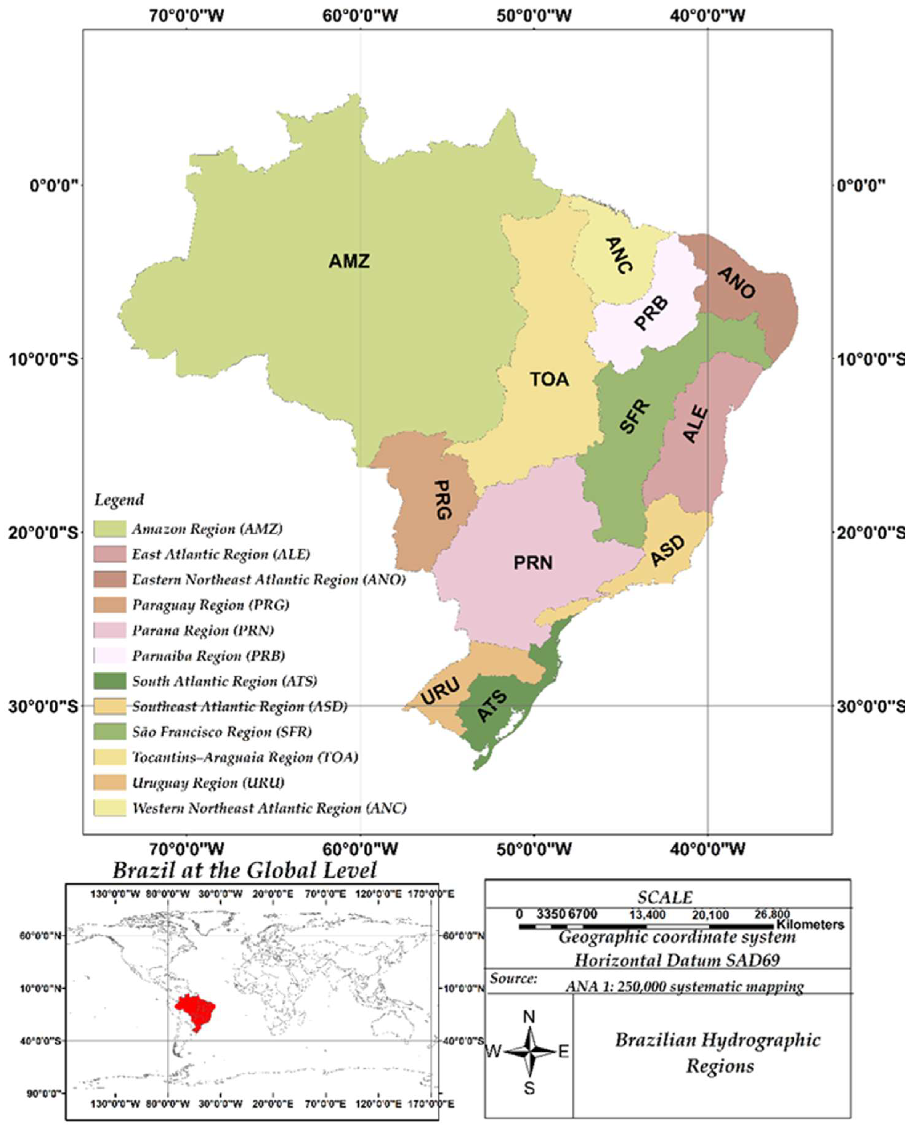
Because of the continental size of the country, Brazil is divided into 12 hydrographic regions for water resources planning and management, as illustrated in Figure 1: Amazon (AMZ), Western Northeast Atlantic (ANC), Parnaíba (PNB), Eastern Northeast Atlantic (ANO), Tocantins–Araguaia (TOA), São Francisco (SFO), East Atlantic (ALE), Paraguai (PRG), Paraná (PRN), Southeast Atlantic (ASD), South Atlantic (ATS), and Uruguai (URU). These hydrographic regions are used in this study as independent spatial units, acting as the basis for the analysis of trend detection in annual streamflow extremes.
2.2. Streamflow Data
This study employed daily streamflow data from 1106 selected gauges located across Brazil. Only gauges with at least 30 years of record length and with at least 5 years of data in the period 2000–2015 were selected for the study. The latter criterion was used to avoid working with gauges that had been inactive for many years.
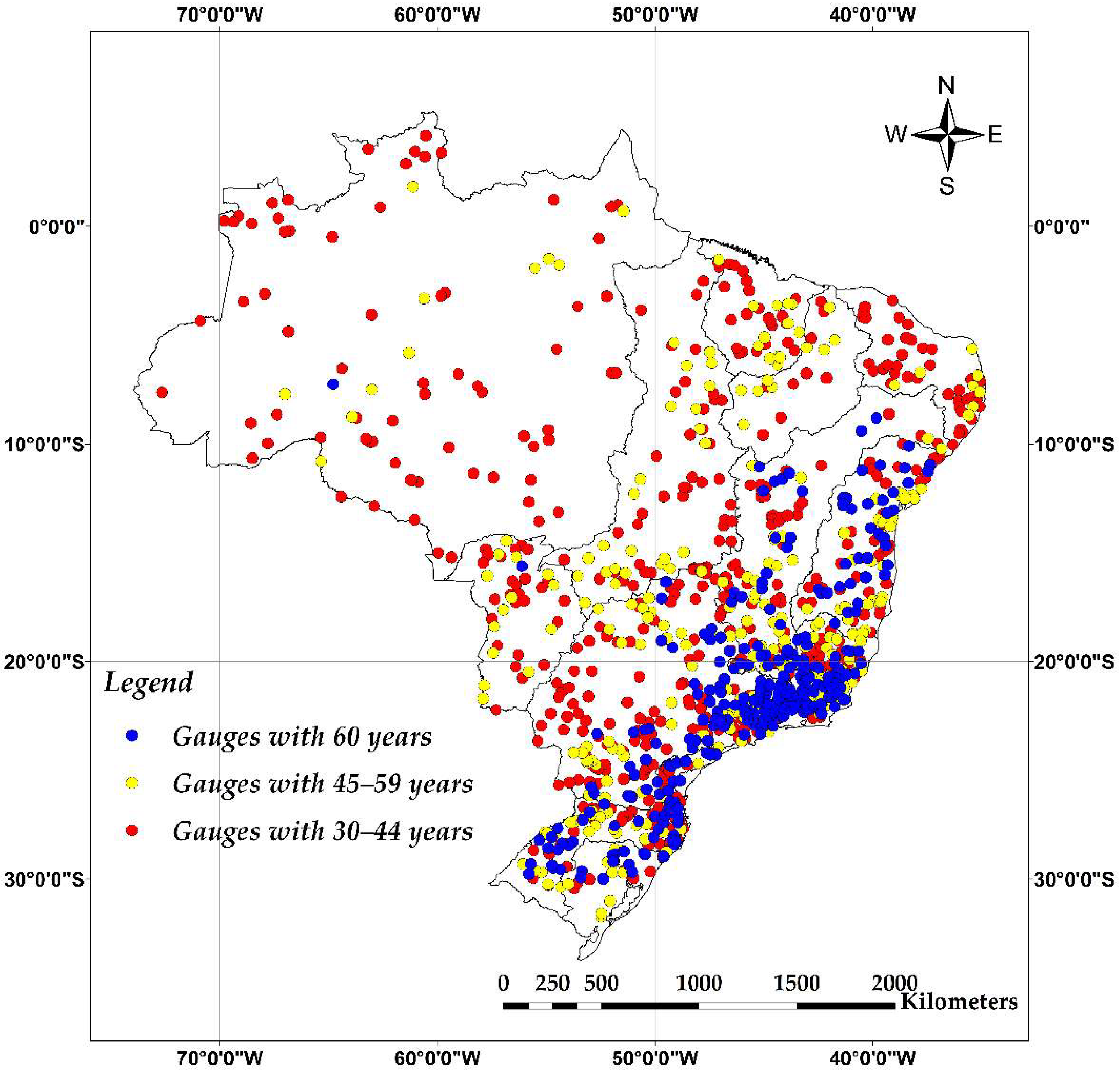
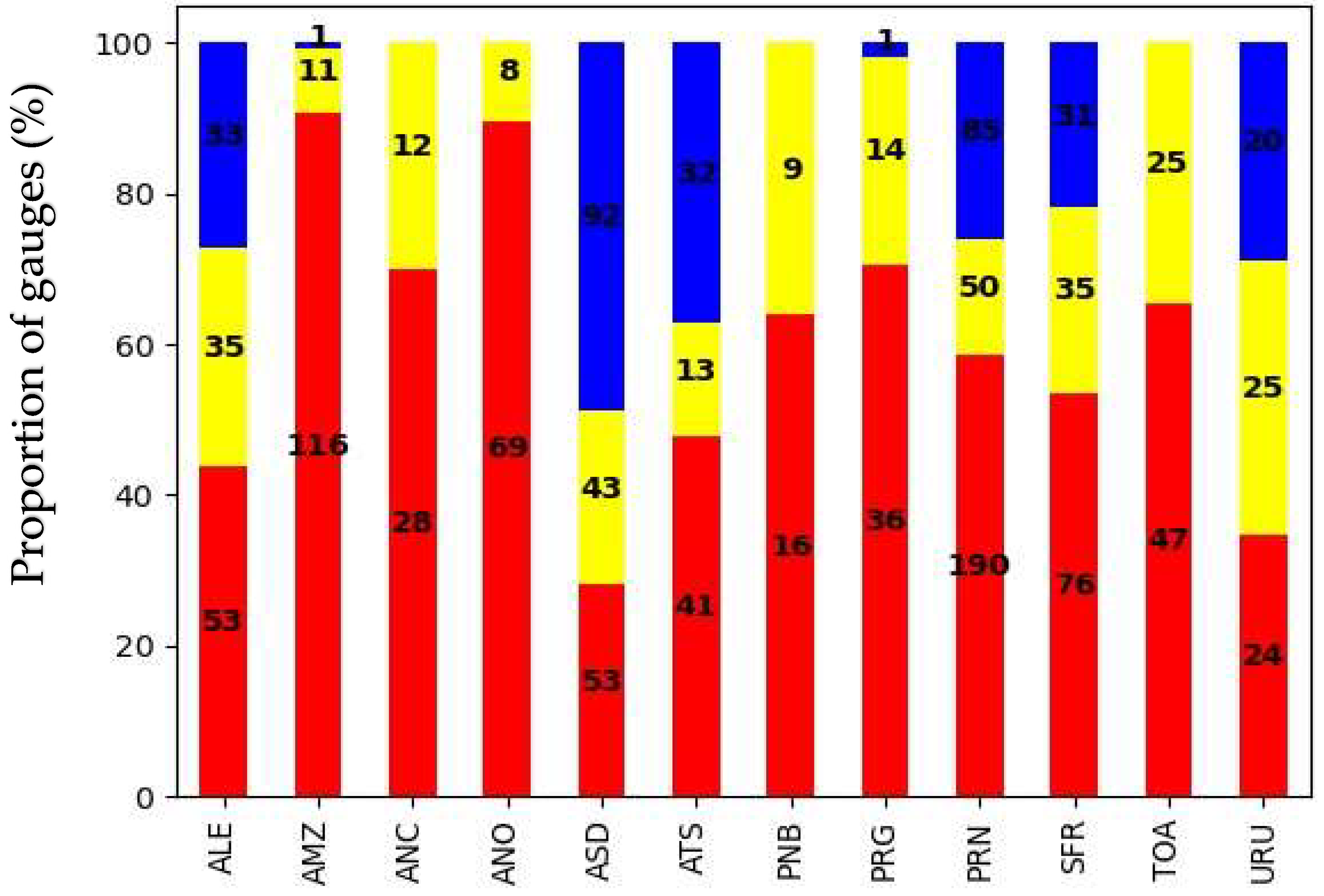
Figure 2 presents the location of these gauges, where colors indicate record length. Gauges with a long record length are located primarily in the eastern part of Brazil. The longest record length was 92 years. A quarter of the 1106 gauges used in the study has at least 60 years of data, and half have at least 43 years. Catchment sizes range from 12 to 4,670,000 km2 with a median of 3220 km2. The majority (80%) of the gauges have drainage area less than 20,000 km2, and only 10% have drainage areas larger than 50,000 km2. Figure 3 presents the proportion and number of gauges for each hydrographic region stratified by classes of record length. The PRN hydrographic region has almost 30% (325) of all gauges used in the study, but the ASD has the most gauges (92) with a record length greater than 60. The PNB hydrographic region has the smallest number of gauges with only 16.
2.3. Streamflow Indices
Table 1 presents eight indices that were selected to describe different aspects of measured daily streamflow. The use of such indices is important to provide a clear picture of possible changes in flow patterns and how these changes may impact different parts of society. For instance, changes in low flows can have an impact on the reliability of water supply and hydroelectric generation, whereas changes in high flows may dramatically impact flood risk.
2.4. Presence of Reservoirs
Although attribution is not the objective of this study, we decided to perform the analysis for two datasets, one with the whole set of selected gauges and another that contains only gauges that are not affected by reservoirs.
To accomplish this task, we used a database that contains information about natural and artificial water bodies in Brazil (MDA). There are 240,899 water bodies currently registered in the MDA, summing up to a total surface area of 173,749.56 km2. About a quarter of them (66,372) are composed of natural water bodies with a total area of 128,165.89 km2. The remaining are artificial water bodies that account for a total area of 45,583.76 km2.
The criterion adopted to decide whether reservoirs located upstream potentially affect the flows of a gauge was the degree of regulation (DoR). DoR is defined as the ratio between the sum of all reservoirs’ storage capacity located upstream and the long-term mean annual flow [87,88,89] given by:
where is the storage capacity of reservoir i located upstream at gauge j, is the number of reservoirs upstream, and is the mean annual streamflow, in volume, at gauge j.
There is no predefined DoR threshold value above which one can say flows are affected by reservoirs upstream. Here, we follow [89,90] and declare that gauges with are unaffected by the presence of reservoirs. Out of the 1106 gauges selected for the study, 670 were considered unaffected by reservoirs, about 60% of the total number of gauges. The choice of the threshold of 0.02 for DoR is subjective, and the most appropriate value for this analysis may depend on the flow index of interest. This threshold value should be better evaluated in future assessments. Figure 4 provides a general picture of the values of DoR at the national scale. In this case, DoR was computed for each river stretch of the national river network.
2.5. Trend Detection Framework
This section provides the methodological steps used in this study to identify trends and estimate their magnitudes. Figure 5 gives a general overview of the strategy used. This section continues with a description of the statistical test used to assess trend significance and the estimator of the magnitude of a trend, followed by a discussion on the methods used to deal with both serial correlation and multiplicity of tests.
2.5.1. Mann–Kendall Trend Test
The Mann–Kendall (MK) trend test [91,92] was adopted in this study to identify statistically significant monotonic increasing or decreasing trends. The MK test is a nonparametric approach that does not require any assumption about the probabilistic model. The test is also applicable to data containing outliers or nonlinear trends [46]. The MK test is widely used in trend detection studies because it is distribution-free and robust against outliers and has a higher power for non-normally distributed data [63,93]. In addition, it has been used in most previous streamflow trend analyses [7,48,52,94]. Considering {x1, x2, x3, . . ., xn} a time series of length n, then the MK test statistic S is given by:
where
The null hypothesis H0 for the test is ‘‘there is no trend in the time series”. If H0 is true, then S is normally distributed with zero mean and variance ,
where n is the number of data points, m is the number of tied groups, and ti is the number of ties of size i. A tied group is a set of sample data having the same values. In cases where the sample size n is greater than 10, S is approximately normally distributed, which justifies the use of the standard normal variate, Z, as the test statistic:
where the unity in the numerator is used for continuity issues in small samples since S is discrete. A positive (negative) value of Z indicates an increasing (decreasing) trend. If or , the null hypothesis that trend is absent can be rejected at α% significance level. In this study, the α significance level was 5%.
2.5.2. Theil–Sen Slope Estimator
Here, we use the Theil–Sen approach (TS) [95] to estimate the actual magnitude of the trend, , which is important to understand the practical implications of detected trends and to evaluate the costs of the associated impacts. The nonparametric TS estimator of the magnitude of trend is based on the slope of all distinct pairs of observations in a sample of size n, denoted here as :
where xi and xj are the data values at times . The decadal relative TS slope estimator of β is given by:
where is the median of all values of and is the sample mean.
2.5.3. Adjustment for Autocorrelated Data
The MK test assumes that the input data are serially independent. The presence of a positive serial correlation in the data structure makes the test more liberal, meaning it rejects the null hypothesis more often than its significance level suggests [58,60,96,97].
The presence of serial correlation is assessed by a statistical test based on the following approximation of the 95% confidence interval for the population lag-1 serial correlation [98,99,100]:
The true and unknown lag-1 serial correlation is usually estimated using the estimator r1, given by:
where is the sample mean. If the sample lag-1 serial correlation, r1, falls within the interval given by Equation (8), the sample data are assumed to be serially independent. Otherwise, the sample data are considered serially correlated.
As the estimator of the autocorrelation r1 has a downward bias (negatively) [92], we also use a bias-corrected estimator based on [101]:
In order to eliminate the influence of serial correlation on the MK test, von Storch [58] proposed the removal of the serial correlation component from the time series based on the assumption that the series comes from a lag-1 autoregressive process, AR(1). The MK test is then applied to the modified series to assess the significance of a possible trend. The PW strategy is very popular in trend detection studies, which accounts for serial correlation.
Yue and Wang [97], as well as Yue at al. [102], showed that the PW procedure can seriously distort the possibility of the MK test to detect a trend. When a trend is present in the series, the estimation of the correlation component of the AR (1) model is inflated. When PW removes the inflated correlation component of the series, it ends up removing part of the trend, causing the distortion in the results of the MK test, reducing the power of the test.
In order to mitigate these limitations, Yue et al. [64] proposed a modified PW procedure called TFPW. In this procedure, the magnitude (slope) of the trend is first estimated, and the original series is detrended. Then the lag-1 serial correlation coefficient of the detrended series is estimated, and the original series is prewhitened using this estimate. Finally, the identified trend is added to the prewhitened series. The Mann–Kendall test is then applied to the resulting series to assess the significance of the trend. The authors argued that the removal of the trend as a first step may allow for a more accurate estimate of the population’s lag-1 autocorrelation coefficient and a subsequent better estimation of the significance of the trend.
The TFPW procedure was considered the solution to the low level of power attributed to the PW strategy. However, later studies [62,65] demonstrated that the sampling uncertainty in the estimation of the trend led to the violation of the type 1 error. In some cases, the TFPW’s inability to control the type 1 error was similar to the MK’s in the original problem.
Önöz et al. [63] proposed a modified TFPW (MTFPW) procedure to better control type 1 error. Both procedures use the estimated serial correlation from the detrended series, , thus avoiding overestimation due to the presence of a trend. However, unlike TFPW, which applies the PW procedure to to obtain a detrended and prewhitened series, , the MTFPW applies the PW procedure to the original series to obtain a trended prewhitened series to which the MK test is applied to assess the significance of the trend. The outline of the MTFPW procedure is as follows:
- Estimate the magnitude of the trend, , using Equation (7).
- Obtain a detrended series, , by removing the estimated trend from of the original series, , where t is the time interval.
- Estimate an unbiased sample autocorrelation (r1) of the detrended series, .
- If r1 is not statistically different from zero, then the MK test is applied to the original series, . Otherwise, the PW procedure is applied to the original series, , to obtain a prewhitened series, .
- Apply the MK test to to check the significance of the trend.
The MTFPW provides a good tradeoff between type 1 and type 2 errors. The TFPW has a much larger statistical power than the PW method, but it fails to control the type 1 error. The MTFPW, based on a relatively small change in the TFPW method, provides a better control of the type 1 error without losing much statistical power.
2.5.4. The Multiplicity Problem
Trend detection studies usually consist of applying simultaneous hypothesis tests at many gauges in a region. A significant level for the local test (one specific gauge) is specified a priori based on the risk of making a type 1 error. Therefore, if the null hypothesis is true, the probability of making a type 1 error for the specific gauge is simply .
When the goal is to detect the proportion of gauges with trends in a region with many gauges, it is important to control the type 1 error for the whole region, not just for each individual gauge. Ignoring the control of the type 1 error for the region results in a violation of the nominal significance level at the regional level. This problem is called multiplicity of hypothesis tests in statistics.
Here, we use the concept of false discovery rate (FDR), first introduced by Benjamini and Hochberg [70] and defined as the expected value of the proportion of false detections among all rejections:
where is the number of gauges where the null hypothesis was mistakenly rejected. The FDR is widely used in the genetics and epidemiology fields, but only recently, it has gained popularity in hydrologic problems [31,66,67,72,103,104].
The Benjamini–Hochberg (BH) procedure that uses the FDR concept is based on the ordered p-values , associated with the hypotheses and the critical values , considered to be equal to . The BH procedure is sequential, meaning the decision to reject or accept the null hypothesis is made gauge by gauge starting from the one with the largest p-value (less evidence to reject the null). If , then all gauges are declared nonstationary; otherwise, the condition is tested until it is true. For the first time , all hypotheses are rejected.
3. Results and Discussion
3.1. Impacts of Serial Correlation and Multiplicity of Tests
This section illustrates the impacts the presence of serial correlation and the multiplicity of hypothesis tests have on trend detection from the MK test. To assess these impacts, we used three different approaches to detect trends in the eight streamflow indices (Table 1): MK, MK-MTFPW, and MK-MTFPW-FDR. The MK approach consists of applying the MK test to the series with no concern for whether observations are correlated or independent or to control the type 1 error at the regional level. The approach denoted as MK-MTFPW, as its name suggests, deals with the presence of autocorrelation using the MTFPW method but ignores the multiplicity issue. Finally, the MK-MTFPW-FDR approach deals with both issues using the FDR to control the type 1 error at the regional level. Both local and regional significance levels used in this study were equal to 5%.
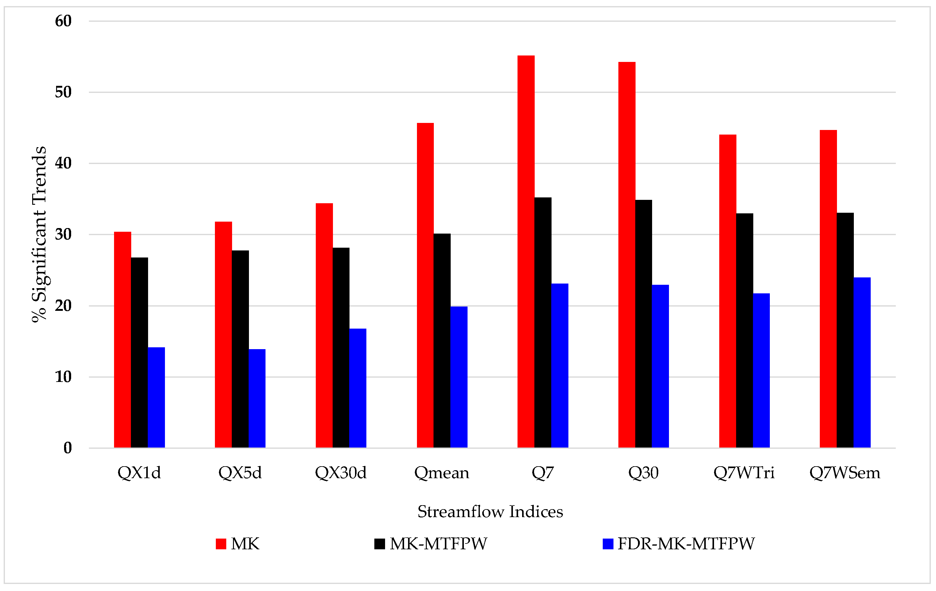
Figure 6 shows the proportion of gauges with a significant trend for each one of the eight streamflow indices using the three different approaches. One can see, as expected, that ignoring the presence of a serial correlation and the control of the type 1 error at the regional level results in a larger proportion of gauges with significant trends, possibly with a large number of false positives, when compared with the other two approaches.
When we compare the results obtained by the MK (red bar) with those obtained by the MK-MTFPW (black bar), the differences are larger for low-flow indices compared with high-flow indices. This makes sense as a serial correlation is much stronger among indices of low flow. These results show the importance of using a procedure to consider the serial correlation when it is present in the data. For instance, the proportion of gauges with significant trends in Q7 series is about 55% if the MK procedure is used but only approximately 35% when the serial correlation is appropriately considered in the analysis. Ignoring the serial correlation can heavily distort the results and may provide a completely different picture of reality.
Ignoring the multiplicity problem when simultaneously applying hypothesis tests for many gauges in a region can also result in large numbers of false positives at the regional level. One can see important differences in the proportion of gauges with significant trends when comparing the MK-MTFPW (black bar) and the MK-MTFPW-FDR (blue bar). However, unlike the differences between the MK and the MK-MTFPW, due to serial the correlation alone, here, these differences are equally proportional regardless of the streamflow indices.
Although results presented in Figure 6 provide an enlightening understanding of the effects of serial correlation and multiplicity in the trend detection, they fail to provide a complete picture of the situation. Neither is the signal of the significant trends explicitly given nor is the spatial distribution of the significant gauges presented on a map.
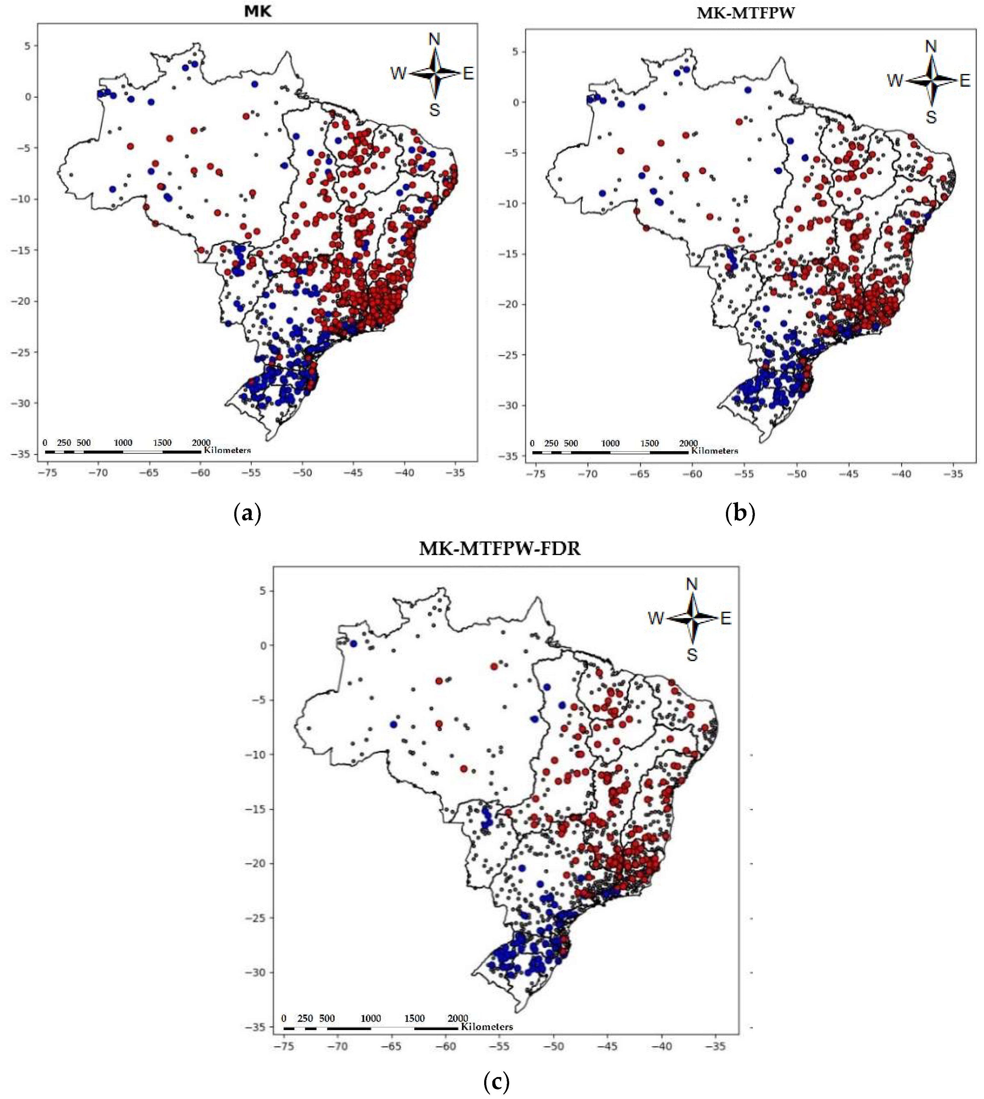
Both the signal of the significant trends and the distribution of gauges on a map are presented in Figure 7. Because of the lack of space, results are presented only for Q7. Red (blue) circles represent gauges with decreasing (increasing) trends, whereas black dots represent gauges with nonsignificant results. The three panels in Figure 5 show the results obtained by each of the three approaches used in the analysis.
Regardless of the approach used, one can notice a clear spatial pattern with the majority of decreasing significant trends happening in the northern and eastern parts of the country, except for the Amazon region, where no clear pattern is identified, and a greater part of gauges with increasing significant trends in the southern part of the country. As we move from the MK results to the MK-MTFPW and MK-MTFPW-FDR results, the density of red or blue circles diminishes, but the spatial consistency remains. In fact, it was observed that the use of the FDR procedure, which controls the expected number of false positives, avoided some regional inconsistencies obtained with the MK and MK-MTFPW, where some gauges located close to each other presented significant trends with different signs. The use of the MK-MTFPW-FDR approach resulted in more clearly identified clusters of gauges with significant trends.
3.2. Trend Analysis in Hydrographic Regions
The previous section showed the impacts that both serial correlation and multiplicity have on the results of trend detection. From this point onwards, all the results presented here were obtained by the MK-MTFPW-FDR approach, which accounts for both issues. Moreover, the control of the type 1 error at the regional level using the FDR procedure was applied separately for each hydrographic region.
Table 2 presents the results in terms of the proportion of gauges with significant trends at the national level for all streamflow indices. The results are stratified based on three classes of record length: short (30–44 years), medium (45–59 years), and long (>60 years), and three classes of relative change per decade: small (), medium (), and large (). Partitioning the results into classes of record length and relative change per decade helps the interpretation of the results.
Gauges with longer record length are associated with more precise results in terms of detection and estimation of trend magnitude since they usually result in tests with more statistical power. Therefore, gauges with large relative changes per decade and long, or at least medium, record lengths stand out from the rest as results are more precise and potential impacts tend to be more relevant due to the magnitude of changes. Water managers and other professionals in charge should study gauges in these classes more carefully and perhaps initiate an assessment of possible impacts in society. Gauges with short record length should be treated carefully as their trend detection results are more uncertain due to low statistical power and the likely overestimation of trend magnitude. Further, gauges with small relative change per decade, at least in a preliminary analysis, are of less concern. For instance, even a small relative change in Q7 in an already water-stressed region may be enough to threaten the water supply system of a community. These discussions, which are out of the scope of this paper, should be kept in mind when interpreting the results. The reader interested in issues related to differences between statistical and practical significance is referred to [105,106,107] for a general discussion and to [64,93,96,108,109] for a hydrological perspective. We just want to make sure that we provide results with enough details so that water managers can identify entire regions or a set of gauges that demand a deeper examination to assess a need for action.
Based on the results presented in Table 2, one can see that the proportion of gauges with significant trends at the national scale is larger for low flows (22–24%) than for high flows (14–16%). When we focus only on large and medium relative changes per decade (), the proportion of significant gauges for low flows (20–23%) is even larger than that for high flows (12–15%). Moreover, at the national scale, low-flow indices seem to be of a greater concern, at least in terms of the magnitude of change, than high flows. This should not be interpreted as changes in high-flow indices cannot be a problem in some specific basins.
A deeper look into the results for the low-flow indices indicates that approximately two-thirds (63–70%) of the gauges with significant trends have a large relative change per decade (). However, only approximately one-fourth (26–30%) of the gauges with significant trends have long record lengths (n > 60). As the record length is strongly associated with the uncertainties in the results, its value is important to understand the degree of confidence we have in these results. Results for low-flow indices presented in Table 2 show that about 30% of the gauges with significant trends have at least a medium relative change per decade () and long record length (n > 60). This proportion of gauges represents about 70 potentially problematic basins with the highest degree of confidence in the results due to the long length of record. If we include gauges with medium record length, the proportion increases from 30% to 50% of the gauges with significant trends, which represents about 130 basins. This statement does not mean that results obtained with short record lengths should not be used, but caution is required.
In addition, the results show that there is a tendency to have a larger proportion of gauges with a decreasing trend than with increasing trends for all indices, especially if the relative change per decade is large. However, this tendency is clearest for low flows. In general, the dominant trend in Brazil points toward drier conditions, although there are some regions that are becoming more humid, as we will show later.
The results from Figure 8 clearly show a large predominance of decreasing significant trends in SFR, PNB, TOA, and ALE hydrographic regions and to a lesser degree in ANC and ANO, regardless of the streamflow indices. All these regions are in northeastern and southeastern Brazil or encompasses part of the Central–Western and Northern parts. Conversely, we find the large majority of positive increasing trends in URU, ATS, and PRG hydrographic regions, all located in the south or the southern part of the Central–Western region. However, the degree of regional predominance is not as strong as the one for negative trends. This general spatial pattern agrees with results previously published for the southern [77,81,82,83,84,110] and for the northeastern and northern parts of Brazil [78,80,82,85].
Although most significant gauges in the AMZ region have increasing trends, except for Q7, for which there is a balance between increasing and decreasing trends, the proportion of gauges with significant trends is small. Finally, one observes a mix of increasing and decreasing significant trends for gauges located in the PRN hydrographic region, which encompasses the south and the southern part of Southeastern Brazil. A further discussion about the spatial distribution of these results is provided in the sequence.
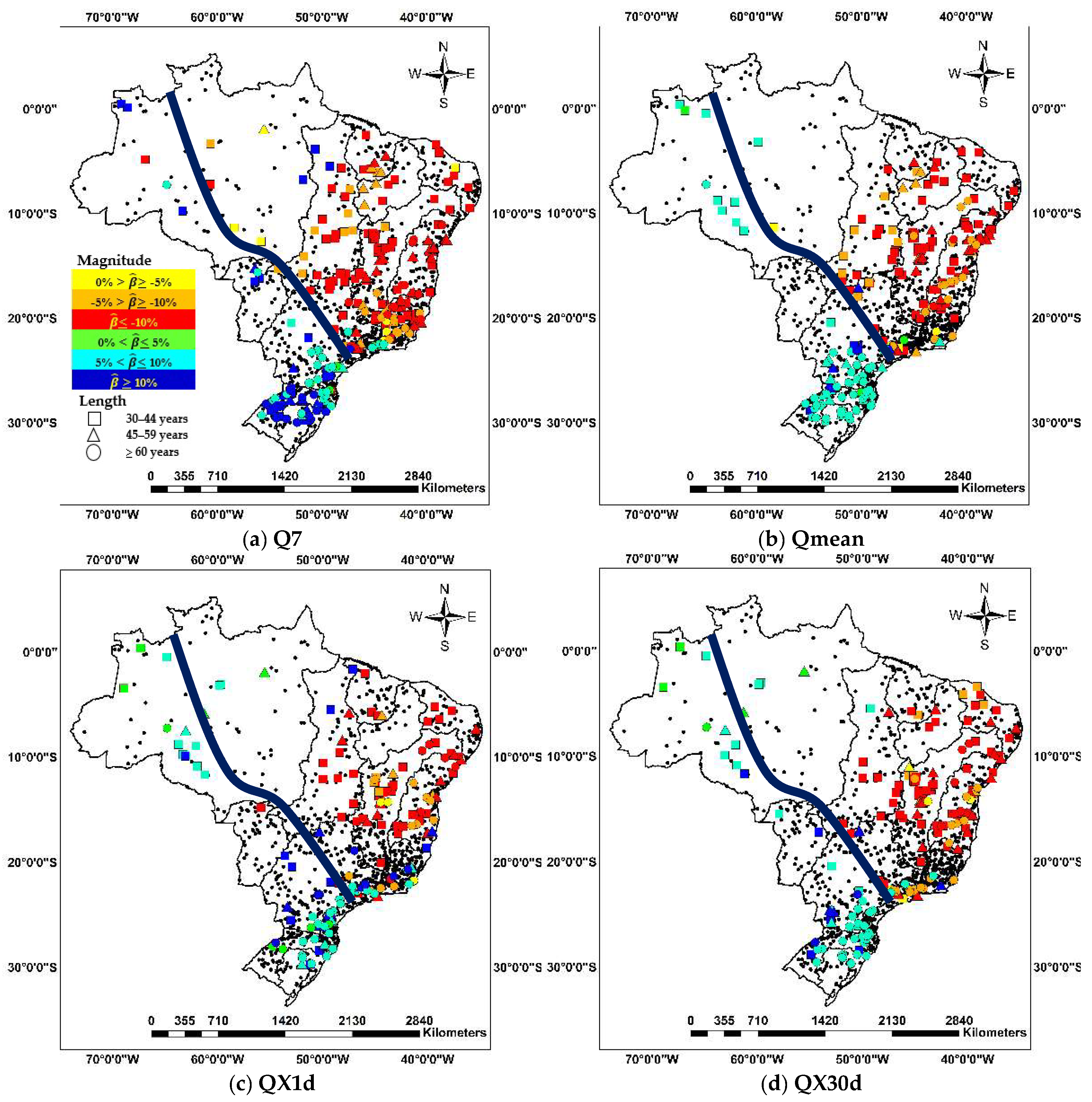
The spatial distribution of the results for the streamflow indices discussed in the previous paragraphs is displayed in Figure 9 with the inclusion of information on the classes of record length and relative change per decade (see legend).
One can see that the majority of the significant trends have medium or large relative change per decade () with a few yellow or green gauges. Except for the Amazon hydrographic region, the country can be divided into two great regions by drawing an NW–SE line that cuts the PRN region in half. Above this line, one predominantly observes gauges with decreasing trends, including those located in the northern half of the PRN region. In the region below this line, which includes the PRG region, one predominantly observes gauges with increasing trends. This general pattern is true not only for the four indices presented in Figure 9 but also for the remaining four indices.
It is worth mentioning that the presence of a large number of gauges with long records and with large or medium relative increasing changes per decade trends for Q7 (dark and light blue circles) in Southern Brazil. The same pattern is observed for high-flow indices but with a smaller proportion of gauges. It is also possible to see a great number of gauges with long records and with large or medium relative decreasing change for Q7 in gauges located mostly in the ASD, northeastern part of PRN, and southern part of both SFR and ALE hydrographic regions. These regions and subregions that contain gauges with long record length, resulting in more precise trend results, and with large or medium relative changes per decade, putting them in a subset of potentially problematic regions, should have the attention of water resources managers, especially in cases of decreasing trends for Q7 and increasing trends for both QX1d and Qx30d.
3.3. Analysis with Gauges Unaffected by Reservoirs
The results presented so far were based on a dataset that contains gauges that are potentially affected by the presence of reservoirs upstream, a fact that may explain, at least partly, the findings of significant trends presented earlier. Although attribution is not the objective of this paper, we decided to provide a view of trend patterns for those gauges that are unaffected by reservoirs. To perform this second part of the analysis, we created a second dataset that contains only gauges that are unaffected by reservoirs.
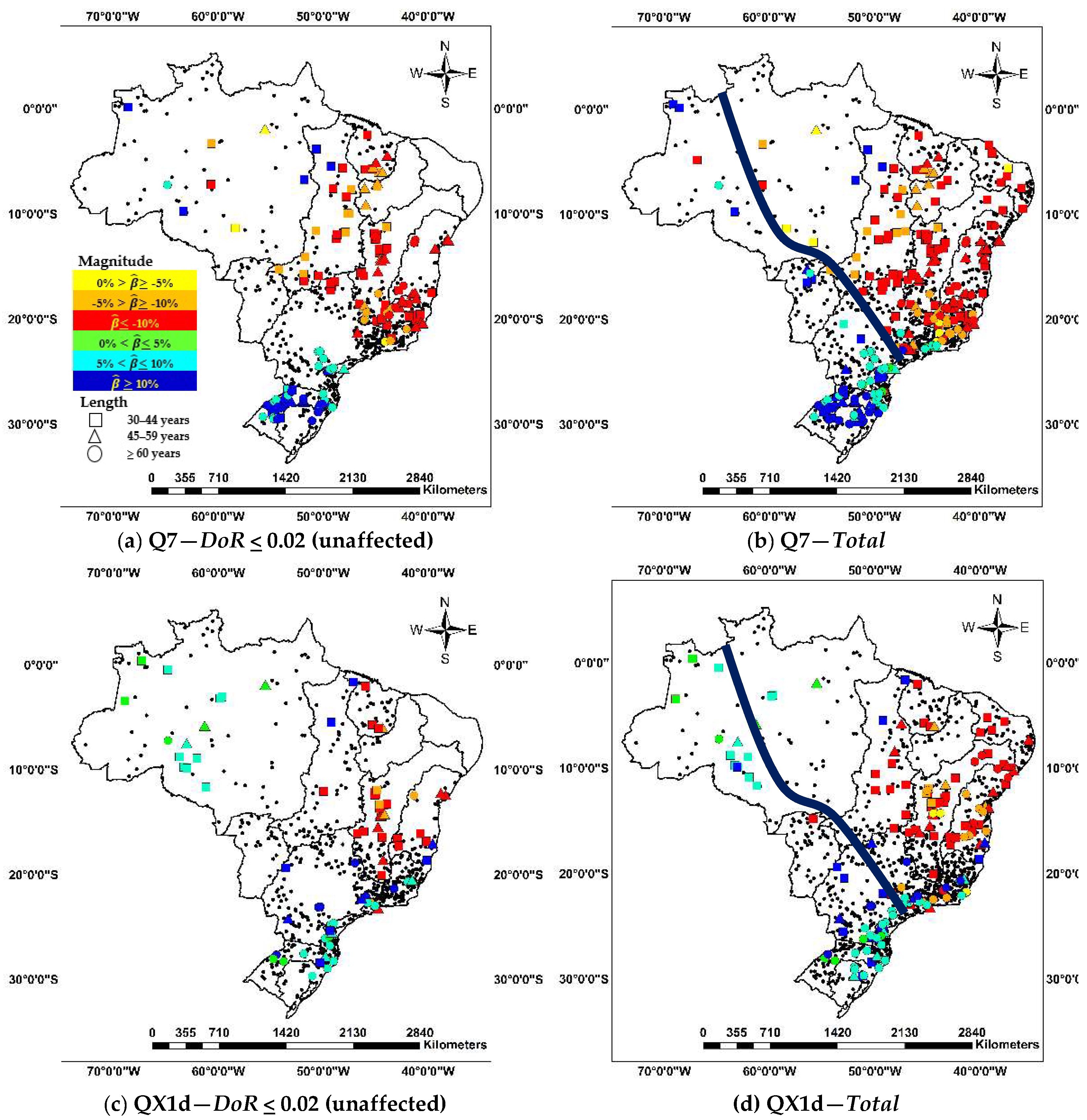
The results of this analysis are presented in Figure 10, which displays the spatial distribution of gauges with significant trends for Q7 and QX1d. Results for two datasets are presented side by side to ease the comparison. Panels (a) and (c) provide the results for gauges that are unaffected by reservoirs, while panels (b) and (d) provide the results for all 1106 gauges.
In general, the spatial pattern obtained in the previous analysis for Q7 and QX1d using all 1106 gauges is still present in the analysis that uses only gauges unaffected by reservoirs. It is possible to say, for instance, that the large number of gauges with increasing trends for Q7 in Southern Brazil is not the result of reservoirs alone as we observe a clear pattern of increasing trends at unaffected gauges. Something similar can be said about the results for QX1d for the same region. In this case, the presence of reservoirs is expected to reduce the annual maximum flows, but we observe increasing trends at gauges both affected and unaffected by the presence of reservoirs.
Figure 10c shows that almost all gauges unaffected by reservoirs located in the SFR, ALE, and ANC regions show a decreasing significant trend for QX1d. This result supports the general conclusion that the decreasing trends for high flows observed in the first part of the analysis cannot be explained solely by the presence of reservoirs.
4. Conclusions
This paper used daily streamflow data from 1106 gauges across the Brazilian territory to assess the significance and estimate the magnitude of changes in eight extreme streamflow indices that cover different and important aspects of flows for water resources planning and management. Unlike most studies carried out in the past using Brazilian hydrological data, the effects of both serial correlation and the multiplicity of hypothesis tests in the regional analysis were assessed and properly considered so as to control the expected number of false positives.
Results on the proportion of gauges with significant trends obtained with three different approaches illustrated the distorting effects serial correlation and multiplicity may have in the analysis, showing how important it is to properly consider these issues in trend detection studies at local and reginal scales.
Trend detection analysis carried out for the 12 hydrographic regions of Brazil, stratified by record length and estimated relative change per decade, provides a comprehensive picture of the existence of trends in flows classified by different levels of confidence in the results, with results obtained for gauges with long record length being the most reliable. Results presented this way are believed to be helpful for water managers, so they can better judge the balance between uncertainty in the estimate and the magnitude of change, both important for making decisions regarding investments in further analysis and development of adaptation strategies.
The estimated proportion of gauges with significant trends in low and high flows was about 23% and 15%, respectively. About two-thirds of all gauges with significant trends for low flow, regardless of their record length, observed relative changes of more than 10% per decade. Results also showed that 50% of gauges with medium or long record lengths observed significant relative changes of at least 5% per decade.
The study identified a very clear spatial pattern. Regardless of the flow index, the majority of gauges with increasing trends were located in the southern part of Brazil, more specifically in the south of the PRN, PRG, and URU hydrographic regions, while the large majority of gauges with decreasing trends were found to the north of that area. A final analysis based on the concept of degree of regulation (DoR) shows that the spatial pattern of trends is also present when only gauges that are unaffected by reservoirs are used, suggesting that the presence of reservoirs alone cannot explain the increasing trends in high flows observed in the southern gauges or the increasing trends in the low flows observed in the gauges located in the northern hydrographic regions.
Further research is needed to investigate the role of potential natural and human-induced factors in the estimated changes in streamflow extremes. Climate variability and change, as well as human activities, such as agricultural expansion, urbanization, and construction of reservoirs, are all factors that must be examined in an attribution analysis that must be carried out in a more refined spatial scale.
Author Contributions
Conceptualization, S.A.d.S. and D.S.R.J.; methodology, S.A.d.S. and D.S.R.J.; software, S.A.d.S. and D.S.R.J.; validation, S.A.d.S. and D.S.R.J.; formal analysis, S.A.d.S. and D.S.R.J.; investigation, S.A.d.S. and D.S.R.J.; resources, S.A.d.S.; data curation, S.A.d.S.; writing—original draft preparation, S.A.d.S.; writing—review and editing, D.S.R.J.; visualization, D.S.R.J. and S.A.d.S.; supervision, D.S.R.J.; project administration, D.S.R.J.; funding acquisition, D.S.R.J. All authors have read and agreed to the published version of the manuscript.
Funding
This research was funded in part by Coordenação de Aperfeiçoamento de Pessoal de Nível Superior–Brazil (CAPES), finance code 001, Brazilian National Water Agency (ANA), Edital Mudanças Climáticas e Recursos Hídricos No. 19/2015, Conselho Nacional de Desenvolvimento Científico e Tecnológico (CNPq), Chamada Universal MCTI/CNPq No. 01/2016, and Fundação de Apoio à Pesquisa do Distrito Federal, Edital 11/2022.
Data Availability Statement
The daily streamflow data can be obtained from the webservice maintained by the National Water Agency of Brazil (https://telemetriaws1.ana.gov.br/ServiceANA.asmx, accessed on 10 January 2022). The annual time series of the streamflow indices for the 12 hydrographic regions used in the paper are available in a GitHub repository (doi: 10.5281/zenodo.6551909). The scripts used in this study can also be accessed in another GitHub repository (doi: 10.5281/zenodo.6555934).
Acknowledgments
The authors are indebted to Alexandre Michalek, Calvin Creech, Renato Amorim, and three anonymous reviewers for their valuable comments.
Conflicts of Interest
The authors declare no conflict of interest. The funders had no role in the design of the study; in the collection, analyses, or interpretation of data; in the writing of the manuscript; or in the decision to publish the results.
References
- National Academies of Sciences, Engineering, and Medicine. Future Water Priorities for the Nation: Directions for the U.S. Geological Survey Water Mission Area; National Academies Press: Washington, DC, USA, 2018; ISBN 9780309477093. [Google Scholar]
- Milly, P.C.D.; Betancourt, J.; Falkenmark, M.; Hirsch, R.M.; Kundzewicz, Z.W.; Lettenmaier, D.P.; Stouffer, R.J. Climate change—Stationarity is dead: Whither water management? Science 2008, 319, 573–574. [Google Scholar] [CrossRef] [PubMed]
- Serinaldi, F.; Kilsby, C.G. Stationarity is undead: Uncertainty dominates the distribution of extremes. Adv. Water Resour. 2015, 77, 17–36. [Google Scholar] [CrossRef] [Green Version]
- Serinaldi, F.; Kilsby, C.G.; Lombardo, F. Untenable nonstationarity: An assessment of the fitness for purpose of trend tests in hydrology. Adv. Water Resour. 2018, 111, 132–155. [Google Scholar] [CrossRef]
- Salas, J.D.; Obeysekera, J.; Vogel, R.M. Techniques for assessing water infrastructure for nonstationary extreme events: A review. Hydrol. Sci. J. 2018, 63, 325–352. [Google Scholar] [CrossRef]
- IPCC. IPCC, 2021: Summary for policymakers. In Climate Change 2021: The Physical Science Basis. Contribution of Working Group I to the Sixth Assessment Report of the Intergovernmental Panel on Climate Change; Masson-Delmotte, V., Zhai, P., Pirani, A., Conn, S.L., Eds.; IPCC: Geneva, Switzerland, 2021. [Google Scholar]
- Su, L.; Miao, C.; Kong, D.; Duan, Q.; Lei, X.; Hou, Q.; Li, H. Long-term trends in global river flow and the causal relationships between river flow and ocean signals. J. Hydrol. 2018, 563, 818–833. [Google Scholar] [CrossRef]
- Zhao, W.; Du, H.; Wang, L.; He, H.S.; Wu, Z.; Liu, K.; Guo, X.; Yang, Y. A Comparison of recent trends in precipitation and temperature over western and eastern eurasia: Differences of climate change between western and eastern eurasia. Q. J. R. Meteorol. Soc. 2018, 144, 604–613. [Google Scholar] [CrossRef]
- Wang, W.; Zhu, Y.; Liu, B.; Chen, Y.; Zhao, X. Innovative variance corrected sen’s trend test on persistent hydrometeorological data. Water 2019, 11, 2119. [Google Scholar] [CrossRef] [Green Version]
- Luke, A.; Vrugt, J.A.; AghaKouchak, A.; Matthew, R.; Sanders, B.F. Predicting nonstationary flood frequencies: Evidence supports an updated stationarity thesis in the United States. Water Resour. Res. 2017, 53, 5469–5494. [Google Scholar] [CrossRef]
- Vogel, R.M.; Rosner, A.; Kirshen, P.H. Brief Communication: Likelihood of Societal preparedness for global change: Trend detection. Nat. Hazards Earth Syst. Sci. 2013, 13, 1773–1778. [Google Scholar] [CrossRef] [Green Version]
- Rosner, A.; Vogel, R.M.; Kirshen, P.H. A Risk-based approach to flood management decisions in a nonstationary world. Water Resour. Res 2014, 50, 1928–1942. [Google Scholar] [CrossRef]
- Doocy, S.; Daniels, A.; Murray, S.; Kirsch, T.D. The human impact of floods: A historical review of events 1980–2009 and systematic literature review. PLoS Curr. 2013. [Google Scholar] [CrossRef]
- Read, L.K.; Vogel, R.M. Reliability, return periods, and risk under nonstationarity. Water Resour. Res. 2015, 51, 6381–6398. [Google Scholar] [CrossRef]
- Svensson, C.; Kundzewicz, W.Z.; Maurer, T. Trend detection in river flow series: 2. Flood and low-flow index series/Détection de tendance dans des séries de débit fluvial: 2. Séries d’indices de crue et d’étiage. Hydrol. Sci. J. 2005, 50, 824. [Google Scholar] [CrossRef] [Green Version]
- Kundzewicz, Z.W.; Mata, L.J.; Arnell, N.W.; Döll, P.; Jimenez, B.; Miller, K.; Oki, T.; Şen, Z.; Shiklomanov, I. The implications of projected climate change for freshwater resources and their management. Hydrol. Sci. J. 2008, 53, 3–10. [Google Scholar] [CrossRef]
- Kundzewicz, Z.W.; Robson, A.J. Change detection in hydrological records—A review of the methodology/revue méthodologique de la détection de changements dans les chroniques hydrologiques. Hydrol. Sci. J. 2004, 49, 7–19. [Google Scholar] [CrossRef]
- Villarini, G.; Smith, J.A.; Serinaldi, F.; Bales, J.; Bates, P.D.; Krajewski, W.F. Flood frequency analysis for nonstationary annual peak records in an urban drainage basin. Adv. Water Resour. 2009, 32, 1255–1266. [Google Scholar] [CrossRef]
- Rice, J.S.; Emanuel, R.E.; Vose, J.M.; Nelson, S.A.C. Continental US streamflow trends from 1940 to 2009 and their relationships with watershed spatial characteristics. Water Resour. Res. 2015, 51, 6262–6275. [Google Scholar] [CrossRef]
- Rodgers, K.; Roland, V.; Hoos, A.; Crowley-Ornelas, E.; Knight, R. An analysis of streamflow trends in the southern and southeastern US from 1950–2015. Water 2020, 12, 3345. [Google Scholar] [CrossRef]
- Mastin, M.C.; Konrad, C.P.; Veilleux, A.G.; Tecca, A.E. Magnitude, frequency, and trends of floods at gaged and ungaged sites in Washington, based on data through water year 2014. Sci. Investig. Rep. 2016. [Google Scholar] [CrossRef] [Green Version]
- Tamaddun, K.; Kalra, A.; Ahmad, S. Identification of streamflow changes across the continental united states using variable record lengths. Hydrology 2016, 3, 24. [Google Scholar] [CrossRef] [Green Version]
- Ishak, E.H.; Rahman, A.; Westra, S.; Sharma, A.; Kuczera, G. Evaluating the non-stationarity of australian annual maximum flood. J. Hydrol. 2013, 494, 134–145. [Google Scholar] [CrossRef]
- Zhang, X.S.; Amirthanathan, G.E.; Bari, M.A.; Laugesen, R.M.; Shin, D.; Kent, D.M.; MacDonald, A.M.; Turner, M.E.; Tuteja, N.K. How streamflow has changed across australia since the 1950s: Evidence from the network of hydrologic reference stations. Hydrol. Earth Syst. Sci. 2016, 20, 3947–3965. [Google Scholar] [CrossRef] [Green Version]
- Potter, N.J.; Chiew, F.H.S.; Frost, A.J. An assessment of the severity of recent reductions in rainfall and runoff in the murray—Darling Basin. J. Hydrol. 2010, 381, 52–64. [Google Scholar] [CrossRef]
- Zhang, X.; Cong, Z. Trends of precipitation intensity and frequency in hydrological regions of China from 1956 to 2005. Glob. Planet. Chang. 2014, 117, 40–51. [Google Scholar] [CrossRef]
- Zhang, Q.; Gu, X.; Singh, V.P.; Xiao, M.; Chen, X. Evaluation of flood frequency under non-stationarity resulting from climate indices and reservoir indices in the East River Basin, China. J. Hydrol. 2015, 527, 565–575. [Google Scholar] [CrossRef]
- Zhang, Q.; Liu, C.; Xu, C.-Y.; Xu, Y.; Jiang, T. Observed trends of annual maximum water level and streamflow during past 130 years in the Yangtze River Basin, China. J. Hydrol. 2006, 324, 255–265. [Google Scholar] [CrossRef]
- Miao, C.Y.; Shi, W.; Chen, X.H.; Yang, L. Spatio-temporal variability of streamflow in the yellow river: Possible causes and implications. Hydrol. Sci. J. 2012, 57, 1355–1367. [Google Scholar] [CrossRef] [Green Version]
- Giuntoli, I.; Maugis, P.; Renard, B. Observed Trends in River Flow Rates in France; ONEMA: Paris, France, 2012; 8p. [Google Scholar]
- Renard, B.; Lang, M.; Bois, P.; Dupeyrat, A.; Mestre, O.; Niel, H.; Sauquet, E.; Prudhomme, C.; Parey, S.; Paquet, E.; et al. Regional methods for trend detection: Assessing field significance and regional consistency. Water Resour. Res. 2008, 44, 1–17. [Google Scholar] [CrossRef] [Green Version]
- Dixon, H.; Lawler, D.M.; Shamseldin, A.Y. Streamflow trends in western britain. Geophys. Res. Lett. 2006, 33. [Google Scholar] [CrossRef]
- Harrigan, S.; Hannaford, J.; Muchan, K.; Marsh, T.J. Designation and trend analysis of the updated UK benchmark network of river flow stations: The UKBN2 dataset. Hydrol. Res. 2018, 49, 552–567. [Google Scholar] [CrossRef] [Green Version]
- Petrow, T.; Merz, B. Trends in flood magnitude, frequency and seasonality in Germany in the period 1951–2002. J. Hydrol. 2009, 371, 129–141. [Google Scholar] [CrossRef] [Green Version]
- Yeste, P.; Dorador, J.; Martin-Rosales, W.; Molero, E.; Esteban-Parra, M.J.; Rueda, F.J. Climate-driven trends in the streamflow records of a reference hydrologic network in Southern Spain. J. Hydrol. 2018, 566, 55–72. [Google Scholar] [CrossRef]
- Martínez-Fernández, J.; Sanchez, N.; Herrero-Jimenez, C.M. Recent trends in rivers with near-natural flow regime: The case of the river headwaters in Spain. Prog. Phys. Geogr. 2013, 37, 685–700. [Google Scholar] [CrossRef]
- Cigizoglu, H.K.; Bayazit, M.; Önöz, B. Trends in the maximum, mean, and low flows of turkish rivers. J. Hydrometeorol. 2005, 6, 280–290. [Google Scholar] [CrossRef]
- Murphy, C.; Harrigan, S.; Hall, J.; Wilby, R.L. Climate-driven trends in mean and high flows from a network of reference stations in Ireland. Hydrol. Sci. J. 2013, 58, 755–772. [Google Scholar] [CrossRef]
- Piniewski, M.; Marcinkowski Pawełand Kundzewicz, Z.W. Trend detection in river flow indices in Poland. Acta Geophys. 2018, 66, 347–360. [Google Scholar] [CrossRef] [Green Version]
- Zhang, X.; Harvey, K.D.; Hogg, W.D.; Yuzyk, T.R. Trends in canadian streamflow. Water Resour. Res. 2001, 37, 987–998. [Google Scholar] [CrossRef]
- Khaliq, M.N.; Ouarda, T.B.M.J.; Gachon, P. Identification of temporal trends in annual and seasonal low flows occurring in canadian rivers: The effect of short- and long-term persistence. J. Hydrol. 2009, 369, 183–197. [Google Scholar] [CrossRef]
- Huziy, O.; Sushama, L.; Khaliq, M.N.; Laprise, R.; Lehner, B.; Roy, R. Analysis of streamflow characteristics over northeastern canada in a changing climate. Clim. Dyn. 2013, 40, 1879–1901. [Google Scholar] [CrossRef] [Green Version]
- Dethier, E.N.; Sartain, S.L.; Renshaw, C.E.; Magilligan, F.J. Spatially coherent regional changes in seasonal extreme streamflow events in the united states and Canada since 1950. Sci. Adv. 2020, 6, eaba5939. [Google Scholar] [CrossRef]
- Wang, W.; Van Gelder, P.H.A.J.M.; Vrijling, J.K. Detection of changes in streamflow series in Western Europe over 1901–2000. Water Sci. Technol. Water Supply 2005, 5, 289–299. [Google Scholar] [CrossRef]
- Hannaford, J.; Buys, G.; Stahl, K.; Tallaksen, L.M. The influence of decadal-scale variability on trends in long European streamflow records. Hydrol. Earth Syst. Sci. 2013, 17, 2717–2733. [Google Scholar] [CrossRef] [Green Version]
- Stahl, K.; Hisdal, H.; Hannaford, J.; Tallaksen, L.M.; van Lanen, H.A.J.; Sauquet, E.; Demuth, S.; Fendekova, M.; Jódar, J. Streamflow trends in Europe: Evidence from a dataset of near-natural catchments. Hydrol. Earth Syst. Sci. 2010, 14, 2367–2382. [Google Scholar] [CrossRef] [Green Version]
- Hall, J.; Arheimer, B.; Borga, M.; Brázdil, R.; Claps, P.; Kiss, A.; Kjeldsen, T.R.; Kriaučiūnienė, J.; Kundzewicz, Z.W.; Lang, M.; et al. Understanding flood regime changes in europe: A state-of-the-art assessment. Hydrol. Earth Syst. Sci. 2014, 18, 2735–2772. [Google Scholar] [CrossRef] [Green Version]
- Madsen, H.; Lawrence, D.; Lang, M.; Martinkova, M.; Kjeldsen, T.R. Review of trend analysis and climate change projections of extreme precipitation and floods in Europe. J. Hydrol. 2014, 519, 3634–3650. [Google Scholar] [CrossRef] [Green Version]
- Kundzewicz, Z.W.; Graczyk, D.; Maurer, T.; Pińskwar, I.; Radziejewski, M.; Svensson, C.; Szwed, M. Trend detection in river flow series: 1. Annual maximum flow/Détection de tendance dans des séries de débit fluvial: 1. Débit maximum annuel. Hydrol. Sci. J. 2005, 50, 810. [Google Scholar] [CrossRef]
- Milly, P.C.D.; Dunne, K.A.; Vecchia, A.V. Global pattern of trends in streamflow and water availability in a changing climate. Nature 2005, 438, 347–350. [Google Scholar] [CrossRef]
- Do, H.X.; Westra, S.; Leonard, M. A global-scale investigation of trends in annual maximum streamflow. J. Hydrol. 2017, 552, 28–43. [Google Scholar] [CrossRef]
- Bürger, G. On trend detection. Hydrol. Process. 2017, 31, 4039–4042. [Google Scholar] [CrossRef]
- Serinaldi, F.; Kilsby, C.G. The importance of prewhitening in change point analysis under persistence. Stoch. Environ. Res. Risk Assess. 2016, 30, 763–777. [Google Scholar] [CrossRef] [Green Version]
- Serinaldi, F.; Kilsby, C. Understanding persistence to avoid underestimation of collective flood risk. Water 2016, 8, 152. [Google Scholar] [CrossRef] [Green Version]
- Wang, W.; Chen, Y.; Becker, S.; Liu, B. Variance correction prewhitening method for trend detection in autocorrelated data. J. Hydrol. Eng. 2015, 20, 4015033. [Google Scholar] [CrossRef]
- Cox, D.R.; Stuart, A. Some quick sign tests for trend in location and dispersion. Biometrika 1955, 42, 80. [Google Scholar] [CrossRef] [Green Version]
- Lettenmaier, D.P. Detection of trends in water quality data from records with dependent observations. Water Resour. Res. 1976, 12, 1037–1046. [Google Scholar] [CrossRef]
- von Storch, H. Misuses of statistical analysis in climate research. In Analysis of Climate Variability; Springer: Berlin, Heidelberg, 1995; pp. 11–26. [Google Scholar]
- Douglas, E.M.; Vogel, R.M.; Kroll, C.N. Trends in floods and low flows in the united states: Impact of spatial correlation. J. Hydrol. 2000, 240, 90–105. [Google Scholar] [CrossRef]
- Yue, S.; Wang, C. The influence of serial correlation on the mann-whitney test for detecting a shift in median. Adv. Water Resour. 2002, 25, 325–333. [Google Scholar] [CrossRef]
- Bayazit, M.; Önöz, B. To prewhiten or not to prewhiten in trend analysis? Hydrol. Sci. J. 2007, 52, 611–624. [Google Scholar] [CrossRef]
- Hamed, K.H. Enhancing the effectiveness of prewhitening in trend analysis of hydrologic data. J. Hydrol. 2009, 368, 143–155. [Google Scholar] [CrossRef]
- Önöz, B.; Bayazit, M. Block bootstrap for mann-kendall trend test of serially dependent data: Block bootstrap for mann-kendall trend test of serially dependent data. Hydrol. Process. 2012, 26, 3552–3560. [Google Scholar] [CrossRef]
- Yue, S.; Pilon, P.; Phinney, B.; Cavadias, G. The influence of autocorrelation on the ability to detect trend in hydrological series. Hydrol. Process. 2002, 16, 1807–1829. [Google Scholar] [CrossRef]
- Hamed, K.H.; Ramachandra Rao, A. A modified mann-kendall trend test for autocorrelated data. J. Hydrol. 1998, 204, 182–196. [Google Scholar] [CrossRef]
- Wilks, D.S. On “field Significance” and the false discovery rate. J. Appl. Meteorol. Clim. 2006, 45, 1181–1189. [Google Scholar] [CrossRef]
- Wilks, D.S. “The stippling shows statistically significant grid points”: How research results are routinely overstated and overinterpreted, and what to do about It. Bull. Am. Meteorol. Soc. 2016, 97, 2263–2273. [Google Scholar] [CrossRef]
- Holm, S. A simple sequentially rejective multiple test procedure. Scand. Stat. Theory Appl. 1979, 6, 65–70. [Google Scholar]
- Hochberg, Y. A sharper bonferroni procedure for multiple tests of significance. Biometrika 1988, 75, 800. [Google Scholar] [CrossRef]
- Benjamini, Y.; Hochberg, Y. Controlling the false discovery rate: A practical and powerful approach to multiple testing. J. R. Stat. Soc. 1995, 57, 289–300. [Google Scholar] [CrossRef]
- Alpert, P. The paradoxical increase of mediterranean extreme daily rainfall in spite of decrease in total values. Geophys. Res. Lett. 2002, 29, 31-1–31-4. [Google Scholar] [CrossRef] [Green Version]
- Ventura, V.; Paciorek, C.J.; Risbey, J.S. Controlling the proportion of falsely rejected hypotheses when conducting multiple tests with climatological data. J. Clim. 2004, 17, 4343–4356. [Google Scholar] [CrossRef] [Green Version]
- Fatichi, S.; Caporali, E. A comprehensive analysis of changes in precipitation regime in tuscany. Int. J. Clim. 2009, 29, 1883–1893. [Google Scholar] [CrossRef]
- Anderson, B.T.; Gianotti, D.J.; Salvucci, G.D. Detectability of historical trends in station-based precipitation characteristics over the continental United States: Station-based precipitation trends. J. Geophys. Res. 2015, 120, 4842–4859. [Google Scholar] [CrossRef]
- Gudmundsson, L.; Seneviratne, S.I. European drought trends. Proc. Int. Assoc. Hydrol. Sci. 2015, 369, 75–79. [Google Scholar] [CrossRef] [Green Version]
- Mallya, G.; Mishra, V.; Niyogi, D.; Tripathi, S.; Govindaraju, R.S. Trends and variability of droughts over the indian monsoon region. Weather Clim. Extrem. 2016, 12, 43–68. [Google Scholar] [CrossRef] [Green Version]
- Genta, J.; Perez-Iribarren, G.; Mechoso, C.R. A recent increasing trend in the streamflow of rivers in Southeastern South America. J. Clim. 1998, 11, 2858–2862. [Google Scholar] [CrossRef]
- Marengo, J.A.; Tomasella, J.; Uvo, C.R. Trends in streamflow and rainfall in Tropical South America: Amazonia, Eastern Brazil, and Northwestern Peru. J. Geophys. Res. 1998, 103, 1775–1783. [Google Scholar] [CrossRef]
- Collischonn, W.; Tucci, C.E.M.; Clarke, R.T. Further evidence of changes in the hydrological regime of the river paraguay: Part of a wider phenomenon of climate change? J. Hydrol. 2001, 245, 218–238. [Google Scholar] [CrossRef]
- Detzel, D.; Bessa, M.; Vallejos, C.; Santos, A.; Thomsen, L.; Mine, M.; Bloot, M.; Estrocio, J. Estacionariedade das afluências às usinas hidrelétricas brasileiras. RBRH 2011, 16, 95–111. [Google Scholar] [CrossRef]
- Doyle, M.E.; Barros, V.R. Attribution of the river flow growth in the Plata Basin. Int. J. Clim. 2011, 31, 2234–2248. [Google Scholar] [CrossRef]
- Alves, B.; Filho, F. Análise de tendências e padrões de variação das séries históricas de vazões do operador nacional do sistema (ONS). RBRH 2013, 18, 19–34. [Google Scholar] [CrossRef]
- Bartiko, D.; Chaffe, P.L.B.; Bonumá, N.B. Nonstationarity in maximum annual daily streamflow series from Southern Brazil. RBRH 2017, 22. [Google Scholar] [CrossRef] [Green Version]
- Chagas, V.B.P.; Chaffe, P.L.B. The role of land cover in the propagation of rainfall into streamflow trends. Water Resour. Res. 2018, 54, 5986–6004. [Google Scholar] [CrossRef]
- Luiz Silva, W.; Xavier, L.N.R.; Maceira, M.E.P.; Rotunno, O.C. Climatological and hydrological patterns and verified trends in precipitation and streamflow in the basins of brazilian hydroelectric plants. Theor. Appl. Clim. 2019, 137, 353–371. [Google Scholar] [CrossRef]
- Agência Nacional de Águas. Conjuntura dos Recursos Hídricos no Brasil 2017: Relatório Pleno; Agência Nacional de Águas: Brasilia, Brazil, 2017; 169p. [Google Scholar]
- Vörösmarty, C.J.; Sharma, K.P.; Fekete, B.M.; Copeland, A.H.; Holden, J.; Marble, J.; Lough, J.A. Lough the storage and aging of continental runoff in large reservoir systems of the world. Ambio 1997, 26, 210–219. [Google Scholar]
- Nilsson, C.; Reidy, C.A.; Dynesius, M.; Revenga, C. Fragmentation and flow regulation of the world’s large river systems. Science 2005, 308, 405–408. [Google Scholar] [CrossRef] [Green Version]
- Lehner, B.; Liermann, C.R.; Revenga, C.; Vörösmarty, C.; Fekete, B.; Crouzet, P.; Döll, P.; Endejan, M.; Frenken, K.; Magome, J.; et al. High-resolution mapping of the world’s reservoirs and dams for sustainable river-flow management. Front. Ecol. Environ. 2011, 9, 494–502. [Google Scholar] [CrossRef] [Green Version]
- Dynesius, M.; Nilsson, C. Fragmentation and flow regulation of river systems in the northern third of the world. Science 1994, 266, 753–762. [Google Scholar] [CrossRef]
- Mann, H.B. Nonparametric tests against trend. Econometrica 1945, 13, 245. [Google Scholar] [CrossRef]
- Kendall, M.G. Time Series, 2nd ed.; Hefner: New York, NY, USA, 1975; 40p. [Google Scholar]
- Yue, S.; Pilon, P.; Cavadias, G. Power of the mann-kendall and spearman’s rho tests for detecting monotonic trends in hydrological series. J. Hydrol. 2002, 259, 254–271. [Google Scholar] [CrossRef]
- Sonali, P.; Nagesh Kumar, D. Review of trend detection methods and their application to detect temperature changes in India. J. Hydrol. 2013, 476, 212–227. [Google Scholar] [CrossRef]
- Sen, P.K. Estimates of the regression coefficient based on kendall’s tau. J. Am. Stat. Assoc. 1968, 63, 1379. [Google Scholar] [CrossRef]
- Yue, S.; Wang, C. The mann-kendall test modified by effective sample size to detect trend in serially correlated hydrological series. Water Resour. Manag. 2004, 18, 201–218. [Google Scholar] [CrossRef]
- Yue, S.; Wang, C.Y. Applicability of prewhitening to eliminate the influence of serial correlation on the mann-kendall test: Technical note. Water Resour. Res. 2002, 38, 4–7. [Google Scholar] [CrossRef]
- Anderson, R.L. Distribution of the serial correlation coefficient. Ann. Math. Stat. 1942, 13, 1–13. [Google Scholar] [CrossRef]
- Yevjevich, V. Probability Statistics in Hydrology; Water Resources Publication: Fort Collins, CO, USA, 1972. [Google Scholar]
- Salas, J.D.; Delleur, J.W.; Yevjevich, V. Applied Modeling of Hydrologic Time Series; Water Resources Publications: Littleton, CO, USA, 1985. [Google Scholar]
- van Giersbergen, N.P.A. On the effect of deterministic terms on the bias in stable AR models. Econ. Lett. 2005, 89, 75–82. [Google Scholar] [CrossRef] [Green Version]
- Yue, S.; Pilon, P.; Phinney, B. Canadian streamflow trend detection: Impacts of serial and cross-correlation. Hydrol. Sci. J. 2003, 48, 51–63. [Google Scholar] [CrossRef]
- Sun, X.; Thyer, M.; Renard, B.; Lang, M. A general regional frequency analysis framework for quantifying local-scale climate effects: A case study of ENSO effects on southeast queensland rainfall. J. Hydrol. 2014, 512, 53–68. [Google Scholar] [CrossRef] [Green Version]
- Amorim, R.S. Detecção de Tendências em Séries de Extremos Hidrológicos Considerando Efeitos de Autocorrelação Temporal e Multiplicidade de Testes. Master’s Dissertation, Universidade de Brasília, Brasília, Brazil, 2018. [Google Scholar]
- Gelman, A.; Stern, H. The difference between “Significant” and “Not Significant” is not itself statistically significant. Am. Stat. 2006, 60, 328–331. [Google Scholar] [CrossRef] [Green Version]
- Sullivan, G.M.; Feinn, R. Using effect size—Or why the p value is not enough. J. Grad. Med. Educ. 2012, 4, 279–282. [Google Scholar] [CrossRef] [Green Version]
- Peeters, M.J. Practical significance: Moving beyond statistical significance. Curr. Pharm. Teach. Learn. 2016, 8, 83–89. [Google Scholar] [CrossRef]
- Clarke, R.T. On the (mis) use of statistical methods in hydro-climatological research. Hydrol. Sci. J. 2010, 55, 139–144. [Google Scholar] [CrossRef]
- Clarke, R.T. How should trends in hydrological extremes be estimated? Trends in hydrological extremes. Water Resour. Res. 2013, 49, 6756–6764. [Google Scholar] [CrossRef]
- Bartiko, D.; Oliveira, D.Y.; Bonumá, N.B.; Chaffe, P.L.B. Spatial and seasonal patterns of flood change across Brazil. Hydrol. Sci. J. 2019, 64, 1071–1079. [Google Scholar] [CrossRef]
Figure 1.
The 12 Brazilian hydrographic regions.

Figure 2.
Location of the streamflow gauges used in the analysis. Red circles indicate gauges with 30–44 years of record length, yellow circles indicate gauges with 45–59 years, and blue circles represent gauges with at least 60 years of data.
Figure 2.
Location of the streamflow gauges used in the analysis. Red circles indicate gauges with 30–44 years of record length, yellow circles indicate gauges with 45–59 years, and blue circles represent gauges with at least 60 years of data.

Figure 3.
Proportion and number of gauges located in the 12 hydrographic regions shown by classes of record length. Red, yellow, and blue bars indicate classes of record length, respectively, 30–44 years, 45–59 years, and at least 60 years of data.
Figure 3.
Proportion and number of gauges located in the 12 hydrographic regions shown by classes of record length. Red, yellow, and blue bars indicate classes of record length, respectively, 30–44 years, 45–59 years, and at least 60 years of data.

Figure 4.
DoR values for all river stretches of the national river network. Gauges with were considered unaffected by the presence of reservoirs.
Figure 4.
DoR values for all river stretches of the national river network. Gauges with were considered unaffected by the presence of reservoirs.

Figure 5.
Flowchart describing a series of steps for Brazilian streamflow trend analysis in this study.
Figure 5.
Flowchart describing a series of steps for Brazilian streamflow trend analysis in this study.

Figure 6.
Proportion (%) of gauges with significant trends for the eight streamflow indices using three different approaches: MK, MK-MTFPW, and MK -MTFPW-FDR.
Figure 6.
Proportion (%) of gauges with significant trends for the eight streamflow indices using three different approaches: MK, MK-MTFPW, and MK -MTFPW-FDR.

Figure 7.
Spatial distribution of trend detection results for Q7. Red (blue) circles represent gauges with decreasing (increasing) trends, while black dots represent gauges with no significant trends. Panels (a–c) present, respectively, the results obtained by the MK, MK-MTFPW, and MK-MTFPW-FDR approaches.

Figure 8.
Trend detection using the MK-MTFPW approach applied to 1106 streamflow gauges in Brazil. Results are shown for each of the 12 hydrographic regions. Red, gray, and blue bars represent significant decreasing, no significant, and significant increasing trends, respectively. Panel (a): Q7; panel (b): Qmean; panel (c): QX1d; panel (d): QX30d.

Figure 9.
Results of trend detection study based on the MK-MTFPW-FDR approach for Q7d (panel (a)), Qmean (panel (b)), QX1d (panel (c)), and QX30d (panel (d)).
Figure 9.
Results of trend detection study based on the MK-MTFPW-FDR approach for Q7d (panel (a)), Qmean (panel (b)), QX1d (panel (c)), and QX30d (panel (d)).

Figure 10.
Spatial distribution of gauges with significant trends for Q7 and QX1d for two different datasets. Panel (a): Q7 for gauges unaffected by reservoirs upstream. Panel (b): Q7 for all 1106 gauges. Panel (c): QX1d for gauges unaffected by reservoirs upstream. Panel (d): QX1d for all 1106 gauges.


Table 1.
Streamflow indices.
| Index | Definition |
|---|---|
| QX1d | Annual maximum daily flow |
| QX5d | Annual maximum 5-day consecutive average flow |
| QX30d | Annual maximum 30-day consecutive average flow |
| Qmean | Mean annual streamflow |
| Q7 | Annual minimum 7-day consecutive average flow |
| Q30 | Annual minimum 30-day consecutive average flow |
| Q7Wtri | Annual minimum 7-day consecutive average flow (wettest trimester) |
| Q7Wsem | Annual minimum 7-day consecutive average flow (wettest semester) |
Table 2.
Percentage of MK trend test results for the 1106 stations across Brazil (NS = nonsignificant and S = significant) for the eight streamflow indices stratified in three classes of record length and three classes of relative change per decade ( .
Table 2.
Percentage of MK trend test results for the 1106 stations across Brazil (NS = nonsignificant and S = significant) for the eight streamflow indices stratified in three classes of record length and three classes of relative change per decade ( .
| Indice | Res | Tot | ||||||||||||||||||
|---|---|---|---|---|---|---|---|---|---|---|---|---|---|---|---|---|---|---|---|---|
| 30–44 years | 45–59 years | >60 years | 30–44 years | 45–59 years | >60 years | 30–44 years | 45–59 years | >60 years | 30–44 years | 45–59 years | >60 years | 30–44 years | 45–59 years | >60 years | 30–44 years | 45–59 years | >60 years | |||
| QX1d | NS | 6% | 1% | 0% | 2% | 0% | 0% | 86% | 2% | 1% | 5% | 3% | 2% | 12% | 6% | 9% | 11% | 7% | 10% | 86% |
| 7% | 3% | 11% | 9% | 27% | 28% | |||||||||||||||
| S | 4% | 1% | 1% | 1% | 0% | 1% | 0% | 0% | 1% | 1% | 1% | 2% | 0% | 0% | 0% | 0% | 0% | 0% | 14% | |
| 6% | 2% | 2% | 3% | 0% | 1% | |||||||||||||||
| QX5d | NS | 7% | 1% | 0% | 2% | 0% | 0% | 9% | 3% | 1% | 5% | 3% | 2% | 10% | 6% | 9% | 11% | 6% | 10% | 87% |
| 8% | 2% | 13% | 10% | 26% | 27% | |||||||||||||||
| S | 4% | 2% | 1% | 0% | 1% | 0% | 0% | 0% | 1% | 1% | 0% | 2% | 0% | 0% | 0% | 0% | 0% | 1% | 13% | |
| 6% | 1% | 2% | 3% | 1% | 1% | |||||||||||||||
| QX30d | NS | 6% | 1% | 0% | 2% | 0% | 0% | 9% | 3% | 2% | 5% | 3% | 2% | 10% | 6% | 11% | 11% | 6% | 8% | 84% |
| 8% | 2% | 13% | 9% | 27% | 25% | |||||||||||||||
| S | 5% | 2% | 1% | 0% | 0% | 0% | 1% | 0% | 2% | 1% | 0% | 3% | 0% | 0% | 0% | 0% | 0% | 0% | 16% | |
| 7% | 1% | 3% | 4% | 1% | 0% | |||||||||||||||
| Qmean | NS | 8% | 2% | 0% | 2% | 0% | 0% | 7% | 3% | 2% | 6% | 2% | 1% | 10% | 8% | 10% | 9% | 5% | 7% | 81% |
| 11% | 2% | 11% | 8% | 28% | 21% | |||||||||||||||
| S | 6% | 2% | 0% | 0% | 0% | 0% | 1% | 1% | 2% | 1% | 1% | 4% | 0% | 0% | 0% | 0% | 0% | 0% | 19% | |
| 8% | 1% | 3% | 6% | 0% | 0% | |||||||||||||||
| Q7 | NS | 10% | 3% | 1% | 4% | 0% | 0% | 7% | 3% | 2% | 3% | 3% | 1% | 8% | 6% | 8% | 7% | 3% | 7% | 77% |
| 14% | 5% | 12% | 7% | 22% | 16% | |||||||||||||||
| S | 7% | 2% | 1% | 2% | 1% | 2% | 1% | 1% | 1% | 0% | 0% | 3% | 0% | 0% | 0% | 0% | 0% | 0% | 23% | |
| 11% | 4% | 3% | 3% | 1% | 0% | |||||||||||||||
| Q30 | NS | 8% | 3% | 0% | 4% | 1% | 0% | 7% | 4% | 2% | 4% | 2% | 1% | 9% | 6% | 9% | 6% | 3% | 6% | 77% |
| 12% | 5% | 13% | 7% | 24% | 16% | |||||||||||||||
| S | 8% | 2% | 1% | 2% | 1% | 1% | 2% | 1% | 1% | 0% | 1% | 3% | 0% | 0% | 0% | 0% | 0% | 0% | 23% | |
| 11% | 4% | 4% | 4% | 0% | 0% | |||||||||||||||
| Q7WTri | NS | 8% | 3% | 0% | 2% | 0% | 0% | 5% | 4% | 2% | 3% | 2% | 1% | 8% | 7% | 9% | 9% | 5% | 8% | 78% |
| 11% | 2% | 12% | 7% | 24% | 21% | |||||||||||||||
| S | 7% | 5% | 2% | 1% | 0% | 0% | 0% | 1% | 2% | 0% | 0% | 2% | 0% | 0% | 0% | 0% | 0% | 0% | 22% | |
| 14% | 1% | 3% | 2% | 1% | 0% | |||||||||||||||
| Q7WSem | NS | 7% | 2% | 0% | 3% | 0% | 0% | 8% | 4% | 2% | 5% | 2% | 2% | 9% | 5% | 8% | 7% | 4% | 7% | 76% |
| 9% | 3% | 13% | 9% | 23% | 19% | |||||||||||||||
| S | 7% | 4% | 1% | 1% | 1% | 1% | 1% | 2% | 2% | 0% | 0% | 2% | 0% | 0% | 1% | 0% | 0% | 0% | 24% | |
| 13% | 2% | 5% | 3% | 1% | 0% | |||||||||||||||
Figure 8 displays the results across the 12 hydrographic regions using stacked bars to show both the proportion and the actual number of gauges with significant trends for each hydrographic regions, and colors to differentiate decreasing (red) from increasing (blue) trends. Only the results for Q7, Qmean, QX1d, and QX30d are presented, but they provide a representation of the situation.
Publisher’s Note: MDPI stays neutral with regard to jurisdictional claims in published maps and institutional affiliations. |
© 2022 by the authors. Licensee MDPI, Basel, Switzerland. This article is an open access article distributed under the terms and conditions of the Creative Commons Attribution (CC BY) license (https://creativecommons.org/licenses/by/4.0/).
Share and Cite
MDPI and ACS Style
Souza, S.A.d.; Reis, Jr., D.S. Trend Detection in Annual Streamflow Extremes in Brazil. Water 2022, 14, 1805. https://doi.org/10.3390/w14111805
AMA Style
Souza SAd, Reis, Jr. DS. Trend Detection in Annual Streamflow Extremes in Brazil. Water. 2022; 14(11):1805. https://doi.org/10.3390/w14111805
Chicago/Turabian StyleSouza, Saulo A. de, and Dirceu S. Reis, Jr. 2022. "Trend Detection in Annual Streamflow Extremes in Brazil" Water 14, no. 11: 1805. https://doi.org/10.3390/w14111805
Note that from the first issue of 2016, this journal uses article numbers instead of page numbers. See further details here.