
Downscaling Microwave Soil Moisture Products with SM-RDNet for Semiarid Mining Areas
by
 ,
,
Xiao Sang
1, 
Jun Li
1,2,*,
Chengye Zhang
1,2,3,
Jianghe Xing
1,
Xinhua Liu
1,
Hongpeng Wang
1 and
Caiyue Zhang
1 1
College of Geoscience and Surveying Engineering, China University of Mining and Technology-Beijing, Beijing 100083, China
2
State Key Laboratory of Coal Resources and Safe Mining, China University of Mining and Technology-Beijing, Beijing 100083, China
3
State Key Laboratory of Water Resource Protection and Utilization in Coal Mining, Beijing 102209, China
*
Author to whom correspondence should be addressed.
Water 2022, 14(11), 1792; https://doi.org/10.3390/w14111792
Submission received: 31 March 2022
/
Revised: 23 May 2022
/
Accepted: 31 May 2022
/
Published: 2 June 2022
(This article belongs to the Section Soil and Water)
Abstract
:Surface soil moisture (SM), as a crucial ecological element, is significant to monitor in semiarid mining areas characterized by aridity and little rainfall. The passive microwave remote sensing, which is not affected by weather, provides more accurate SM information, but the resolution is too coarse for mining areas. The existing downscaling method is usually pointed to natural scenarios like agricultural fields rather than mining areas with high-intensity mining. In this paper, combined with geoinformation related to SM, we designed a convolutional neural network (SM-Residual Dense Net, SM-RDNet) to downscale SMAP/Sentinel-1 Level-2 radiometer/radar soil moisture data (SPL2SMAP_S SM) into 10 m spatial resolution. Based on the in-site measured data, the root mean square error (RMSE) was utilized to verify the downscaling accuracy of SM-RDNet. In addition, we analyzed its performance for different data combinations, vegetation cover types and the advantages compared with random forest (RF). Experimental results show that: (1) The downscaling from the 3 km product with the combination of auxiliary data NDVI + DEM + slope performs best (RMSE 0.0366 m3/m3); (2) Effective data combinations can improve the downscaling accuracy at the range of 0.0477–0.1176 m3/m3 (RMSE); (3) The SM-RDNet shows better spatial completeness, details and accuracy than RF (RMSE improved by 0.0905 m3/m3). The proposed SM-RDNet can effectively obtain the fine-grained SM in semiarid mining areas. Our method bridges the gap between coarse-resolution microwave SM products and ecological applications of small-scale mining areas, and provides data and technical support for future research to explore how the mining effect SM in semiarid mining areas.
1. Introduction
Coal mining inevitably brings a certain amount of impact on the ecological environment in mining areas [1,2,3]. The governments of many countries have formulated corresponding reclamation laws, regulations or other forms of policies to alleviate these impacts [4]. Surface soil moisture (SM) is an essential factor in mining reclamation due to its effect on vegetation growth [5,6,7] and its important role in the land–atmosphere interactions [8,9,10,11], especially in semiarid regions. Therefore, it is critical to obtain reliable and fine-grained distribution of SM in mining areas.
Many studies have demonstrated the capability of remote sensing technologies to retrieve SM products [12], including optical/thermal remote sensing [13,14,15], passive microwave remote sensing [16,17] and active microwave remote sensing [18,19,20,21]. It is generally acknowledged that the passive microwave remote sensing with an L-band has a longer wavelength to penetrate deeper into the canopy and can provide accurate information for SM estimation [16]. Thus, a few passive microwave sensors have been launched which provide daily global SM products, such as the Advanced Microwave Scanning Radiometer for Earth Observing System (AMSR-E) [22], the Advanced Microwave Scanning Radiometer 2 (AMSR-2) [23], the Soil Moisture and Ocean Salinity (SMOS) [24] and the Soil Moisture Active Passive (SMAP) [25]. However, the coarse spatial resolution of the above products prevents them from being applied in small-scale mining areas.
Many scholars have researched to achieve the downscaling of coarse SM products with the help of fine-grained auxiliary data [11,26]. The downscaling methods can be divided into three types according to the dataset used in the fusion process: the optical/thermal and passive microwave data fusion methods, the active and passive microwave data fusion methods and the methods using geoinformation data [27]. For the optical/thermal and microwave data fusion methods, the vegetation indexes and land surface temperature (LST) retrieved from the optical/thermal remote sensing are generally used as auxiliary data to improve the spatial resolution of SM retrieved from the microwave remote sensing [28,29,30]. Additionally, the surface temperature–vegetation index triangular feature space is also applied in SM downscaling because it can distinguish the wet and dry conditions [31,32,33]. Since optical/thermal remote sensing fails in cloudy and rainy weather, this type of method is restricted by weather conditions [10]. For the active and passive microwave data fusion methods, they have been the preferred methods for SM downscaling, since both technologies are sensitive to SM and less affected by weather conditions, and the spatial resolution of active microwaves is high. Various SM datasets were released to the public, such as the SMAP/Sentinel-1 Active¬–Passive SM product (SPL2SMAP_S) [34,35]. Many fusion methods were proposed to merge these two datasets, such as the Bayesian disaggregation method [36,37], the change detection method [38], the optional active/passive retrieval algorithm [39], the baseline algorithm [40] and the Combined Active–Passive algorithm [41]. However, the spatial resolution of SM products using these methods is mostly 1 km, which is not yet suitable for small-scale applications. For the methods using geoinformation data, the topographic features [42], soil properties [43], vegetation characteristics and meteorology are used as the main input data in the downscaling process [44,45,46]. Topography affects SM distribution through soil–water dynamics [47,48], while soil properties affect soil–water storage capacity and possible rates of change [49,50]. Vegetation characteristics affect SM by soil evapotranspiration and the depth of penetration of microwaves into soil [51]. The potential evapotranspiration is also demonstrated to affect the spatial pattern of SM [47,52,53].
Furthermore, the machine learning methods show potential in SM downscaling [54,55,56,57,58]. Liu et al. [59] and Yan et al. [43] compared the performance of various machine learning methods including the artificial neural network (ANN), Bayesian (BAYE), classification and regression trees (CART), K-nearest neighbor (KNN), random forest (RF) and the support vector machine (SVM), and found that RF performed best in most cases. Recently, deep learning technology has been successfully applied in various fields benefiting from the development of computer technologies and the ever-increasing amount of data [60]. Xu et al. [61] applied a convolutional neural network (CNN) to SM downscaling and found that the residual SM value from two SM images with different spatial resolutions performs better than the direct SM value as a predictor.
To meet the requirements of small-scale application scenes, a few scholars have made attempts to obtain SM products with 30 m spatial resolution [19,62,63]. However, existing research established the specific relationship between SM and the impact factors, such as vegetation cover and land surface temperature, for the natural scenarios (e.g., agricultural fields). This relationship in mining scenarios is very different from that in general scenarios. For example, the SM remains high in the open-pit stope despite the absence of vegetation, which makes it difficult to apply existing methods to obtain fine-scale SM for mining scenarios.
In view of the above problems, this paper aims to develop a method for acquiring the fine-grained SM in semiarid mining areas. The method can account for current deficiencies in downscaling SM products for semiarid mining areas. Specifically, we (1) design a convolutional neural network called SM-RDNet to represent the complicated correlation relationship between the SM and spectral, vegetation and topographic features in semiarid mining areas at fine scales, and (2) provide the optimal downscaling option for semiarid mining areas by comparing different combinations of data. This research bridges the gap between coarse-resolution microwave SM products and ecological applications of small-scale semiarid mining areas, and promises to provide fine-grained data to support ecological monitoring in semiarid mining areas.
2. Materials
2.1. Study Area
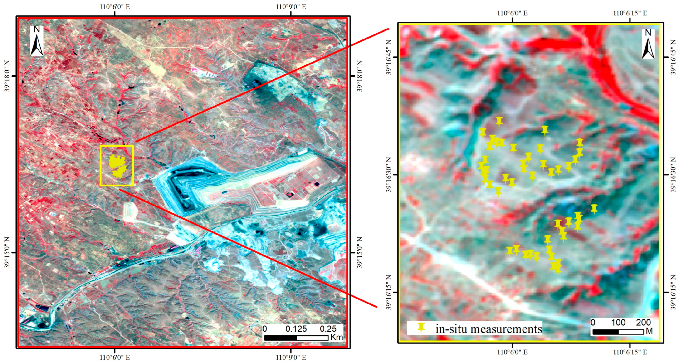
The Shangwan mine area in China’s Ordos Plateau is chosen as the study area (Figure 1). It is located in a semiarid transition region from arid grassland to desert grassland in central Asia, which is characterized by aridity and little rainfall. The average annual precipitation in the region is about 400 mm, while the average annual evaporation is about 7 times as much as precipitation. The average annual temperature is 6.2 °C. The study area has a water-eroded gully landform of the Loess Plateau, with an elevation ranging from 1097 m to 1322 m. It is an ecologically vulnerable area due to the poor climatic environment, and soil erosion is the predominant ecological problem. Coal mining activities in the study area began in the 2000s and contain both open-pit mines and underground mines. The exploitation of coal resources affects the surface/underground ecological environment and leads to a series of environmental problems [64,65,66].
2.2. Data
Experimental datasets include the SPL2SMAP_S SM products, Sentinel-2 remotely sensed images, vegetation index data, topographic data and in situ measurements data.
2.2.1. SPL2SMAP_S SM Products
The SPL2SMAP_S V3 was released in August 2020 to provide SM products at two resolutions, 1 and 3 km, since 31 March 2015, and the geographic coverage spans from 180° W to 180° E and from 60° N to 60° S. It is generated by merging the radiometer brightness temperature data of 40 km SMAP and the radar backscatter data collected by Sentinel-1 based on the SMAP Active–Passive algorithm [34]. The SPL2SMAP_S V3 can be downloaded from the website of the National Snow and Ice Data Center (NSIDC) (https://nsidc.org/data/SPL2SMAP_S, accessed on 17 June 2021). The SPL2SMAP_S V3 on 14 May 2021 is used.
2.2.2. Sentinel-2 Images
The reflectances data collected by the Sentinel-2 satellite is chosen as important auxiliary data since it has a high spatial resolution (10 m), multispectral bands for unprecedented views of the earth and a high revisit frequency (5 days) compared with the other optical images, such as Landsat images (16 days). The wavelength bands we used are listed in Table 1. The Sentinel-2 data acquired on 8 May 2021, which is the closest to the 14 May 2021 that is used. The Sentinel-2 images are provided by the Copernicus program of the European Union, operated by ESA and accessed via the Google Earth Engine (GEE).
2.2.3. Vegetation Index
The vegetation index used in this study is the Normalized Difference Vegetation Index (NDVI) [67], which is calculated based on Sentinel-2 remotely sensed image. It is calculated as Equation (1).
where and are the channel near-infrared reflectance and channel red reflectance, respectively.
2.2.4. Topographic Data
The topographic data include the Digital Elevation Model (DEM) data and the derived slope data. The ASTER GDEM V3, with a spatial resolution of 30 m, is used, and was downloaded from the website of the National Aeronautics and Space Administration (NASA) EarthData (https://earthdata.nasa.gov/, accessed on 17 June 2021).
2.2.5. In Situ Measurement Data
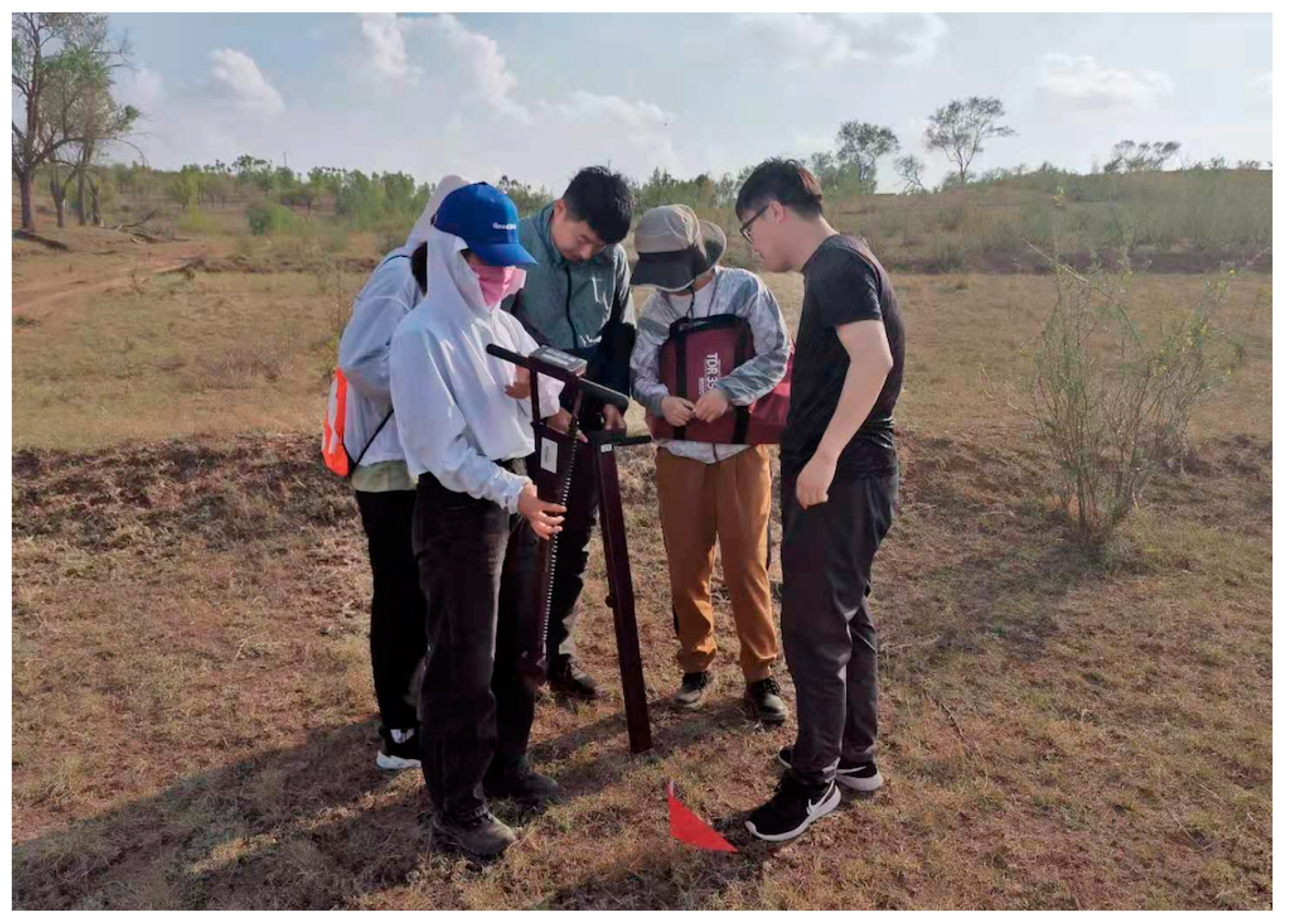
The ground truth SM values were collected on 14 May 2021 in the Shangwan mine area (Figure 1) with the FieldScout TDR 350 Soil Moisture Meter. The instrument can measure the SM value at depths of 3.8 cm, 7.6 cm, 12 cm and 20 cm under the ground surface. Considering that the surface SM monitored by the SPL2SMAP_S data is at a 0–5 cm depth, the SM values at the depth of 3.8 cm were measured in the fieldwork. A total of 54 ground truth SM values were measured within a window of 2 h concerning the Sentinel-1 acquisition time. During the fieldwork, each sample point was measured three times and the average was taken as the truth SM value to verify the accuracy of the downscaled SM value. Figure 2 shows a sample point in the field survey, and Figure 3 demonstrates the spatial distribution of the in situ measurements.
3. Methods
SM downscaling is to transform the SM from a coarse spatial resolution to a fine spatial resolution by means of physical or statistical approaches. The core of SM downscaling is to establish the relationship between the SM and related parameters (e.g., land cover, elevation) at the same place. This paper develops a method based on deep learning to downscale the SM products with auxiliary data to a field-scale spatial resolution. This section presents the details of the deep learning network structure, the implementation of the downscaling process and the accuracy validation for the downscaled SM results.
3.1. SM-RDNet
The SM has a more complex relationship with its impact factors in mining areas than in other scenarios, such as agricultural fields, and this relationship is difficult to accurately express using ordinary statistics models. Convolutional neural networks can well represent a complex relationship. We design a convolutional neural network called SM-Residual Dense Net (SM-RDNet) to downscale the SM products based on a dense residual fully convolutional network structure, as shown in Figure 4. The input of SM-RDNet is the feature variables including the bands of Sentinel-2 images, listed in Table 1, elevation, slope, etc., while its output is the SM values. The detailed procedures are as follows: First, based on a 3 × 3 sliding window, SM-RDNet captures n × 3 × 3 feature blocks from n feature variables. The sliding window allows the neighboring area of the center pixel to be taken into account. Second, the Convolution-ReLU-Batch Normalization (Conv-ReLU-BN) module and two residual dense blocks extract information from feature blocks. With two residual dense blocks, the neural network is further deepened, avoiding the problem of gradient disappearance due to too many layers of the network and increasing the reuse of features [68]. Finally, the number of channels of the output result is changed by 1 × 1 convolution to obtain the final single-band fitting result for this n × 3 × 3 feature block.
3.2. Downscaling Strategy
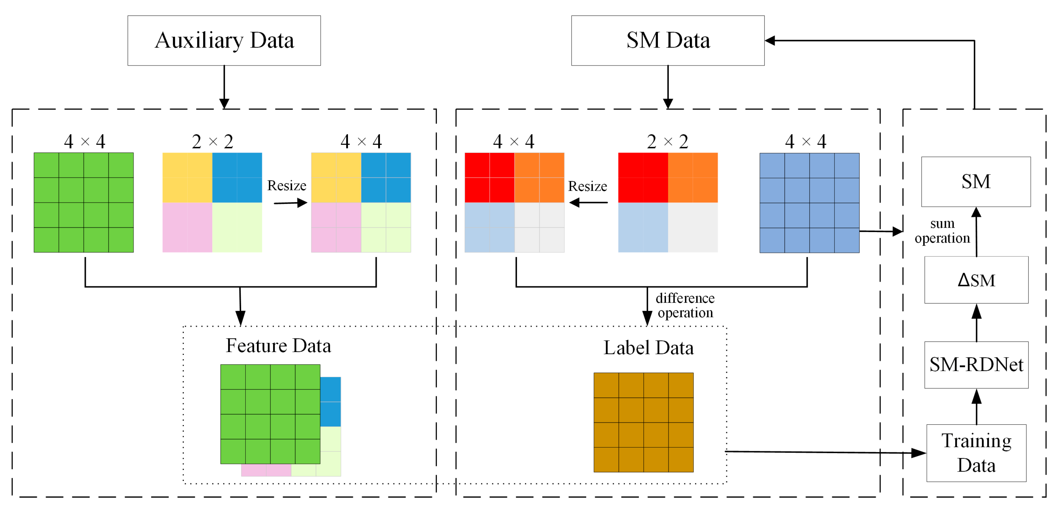
Based on the proposed SM-RDNet, we design the strategy of downscaling the SPL2SMAP_S SM products, and take the residual value (∆SM) between two SM images with different spatial resolutions as the label dataset [61]. Figure 5 shows the flowchart of downscaling strategy, and the detailed process is as follows:
- Preparation of training dataset. The training dataset consists of a label dataset and a feature dataset. The label dataset is the residual value (∆SM) between the SM data with a higher spatial resolution and that with a lower spatial resolution. This process requires the SM product with a lower spatial resolution to be resized to have a higher spatial resolution to perform difference calculation. The feature dataset is obtained by resampling the auxiliary data to the same spatial resolution as the SM data, including Sentinel-2 reflectances, NDVI, elevation and slope. It should be noted that the high-spatial-resolution SM data in the first loop of downscaling is generated by conducting the nearest-neighbor interpolation on the original SM products. For the other loop of downscaling, the SM data we used is the SM predictions from the previous downscaling loops.
- Training of SM-RDNet model. The training dataset is input into the SM-RDNet to generate a prediction model. The prediction model is consecutively trained 200 times and each training evaluates the prediction model by the statistical evaluation indexes root mean square error (RMSE) and coefficient of determination (R2) based on the truth SM values. As the number of training increases, the predicted SM accuracy gradually improves and eventually stabilizes. Finally, the best prediction model is selected. In our experiments, each prediction model has an R2 greater than 0.85 and an RMSE less than 0.004 m3/m3 with respect to the truth SM value.
- Downscaling of SPL2SMAP_S SM products. The auxiliary data are resampled to the target spatial resolution, while the auxiliary data of the feature dataset with the higher spatial resolution are resized to the same dimension, and the two datasets are input into the trained SM-RDNet model to obtain ∆SM. The obtained ∆SM is added to the SM product with the high spatial resolution in the label dataset to obtain the estimated SM values.
- The expansion of spatial resolution in progressively downscaling. To reduce the information loss, the SM with a close resolution to the target is obtained through several downscaling processes. The expansion multiplier in each step is calculated as Equation (2).where Rn_after and Rn_befor are the spatial resolutions after and before the n-th downscaling, respectively, and K is the expansion multiplier.Rn_after = Rn_before/K,In this paper, the expansion multipliers are 3, 3, 3 and 5 in turn for downscaling the 3 km SPL2SMAP_S SM product into the 7.4 m product, which is close to the target spatial resolution (10 m), and are 3, 3 and 5 in turn for downscaling the 1 km SPL2SMAP_S SM products.
- Iterative downscaling process. Each downscaling process includes the training and prediction of the model. In the first training of the model, the higher resolution SM data in the ∆SM (label data) calculation process is generated by conducting the nearest-neighbor interpolation on the original SM products, while the lower resolution SM data is the original SM products. In the n-th training of the model, the higher resolution SM data in the ∆SM (label data) calculation process are the SM predicted results obtained from the (n − 1)-th downscaling, while the lower resolution SM data are the SM predicted results obtained from the (n − 2)-th downscaling. The auxiliary data are used as feature data after the same processing as in step 2. In the n-th model prediction process, the target resolution is calculated by step 4. The auxiliary data processed to the same resolution as the target will be used as input to the prediction model. The output ∆SM is added to the SM predicted from the (n − 1)-th downscaling to obtain the estimated SM values. In particular, the reason we chose iterative downscaling is that Xu et al. showed that the iterative downscaling method performs better than directly downscaling SM products to the target resolution [61].
- When the downscaling is finished, the downscaled SM further needs a resampling to fit the target spatial resolution.
3.3. Accuracy Validation
The accuracy validation of the estimated SM values is conducted by comparing the estimated values with the in situ measurements [69]. Root mean square error (RMSE) is used to evaluate the effectiveness of the downscaled SM Equation (3). A lower value for the RMSE than the estimation value is closer to the ground truth and the downscaled SM value is more accurate.
where Ei and Mi are the i-th estimated and in situ measurement SM values, and n is the total number of validation samples.
4. Results
The proposed SM-RDNet was used to downscale SPL2SMAP_S SM products from km-level resolution to a 10 m resolution. In order to test the performance of SM-RDNet under various scenarios, a few experiments were conducted using a different spatial resolutions of the original SM products and different combinations of the auxiliary datasets.
4.1. Performance of Downscaled SM Derived from 1 Km SPL2SMAP_S SM Products
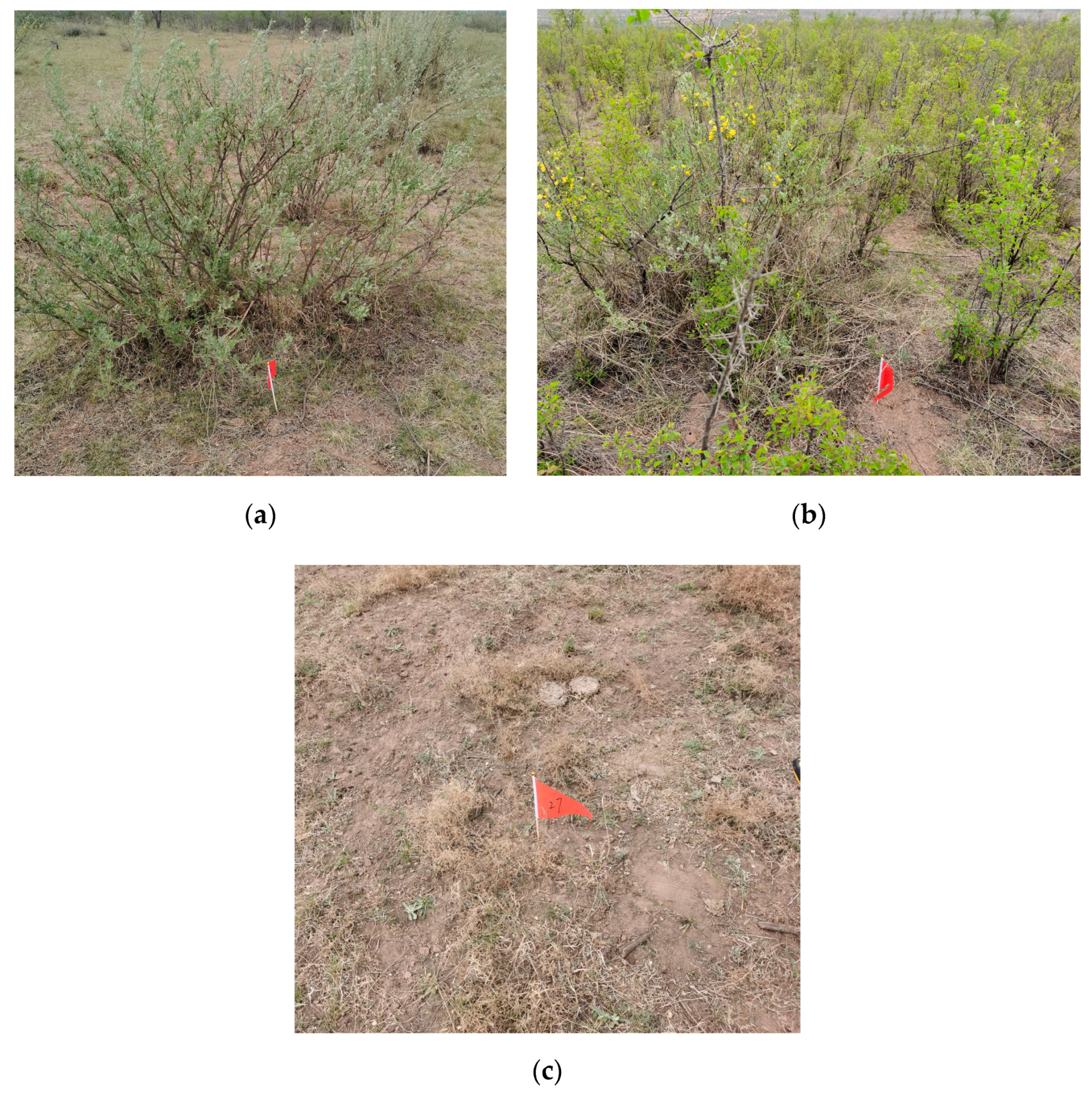
The downscaled SM with various combinations of auxiliary datasets were validated by the in situ measurements. Among auxiliary datasets, the Sentinel-2 reflectances are a necessary dataset, while NDVI, DEM and slope are optional. We further compared the accuracy of the downscaled SMs covered by different types of vegetation, including the Sophora davidii, the Siberian almond tree and the sparse grass. Figure 6 shows the pictures of three types of vegetation in the study area, respectively. The RMSEs of the downscaled SM derived from the 1 km SPL2SMAP_S SM product are summarized, as shown in Table 2.
It can be seen from Table 2 that the average RMSE of the downscaled SMs in the whole area is 0.1266 m3/m3. The accuracy of downscaled SMs in the three subregions alone is better than that in the whole area, which is 0.1208 m3/m3 (RMSE).
The NDVI as auxiliary data alone performs best in four types of vegetation cover. The RMSE is 0.0944 m3/m3 in the whole area; 0.0912 m3/m3 in the Sophora davidii area; 0.0867 m3/m3 in the Siberian almond tree area; 0.0882 m3/m3 in the sparse grass area, respectively. In addition, the combination of NDVI, DEM and slope as auxiliary data provides a higher improvement in accuracy than any other auxiliary datasets.
An integrated analysis of Table 2 demonstrates that the use of NDVI, DEM or slope as an auxiliary dataset can improve the downscaling accuracy to a certain extent compared with using the reflectances alone. Among them, NDVI is most effective in increasing the downscaling accuracy. Furthermore, the performance of downscaling SM in a single vegetation cover is better than in the area with mixed vegetation covers.
4.2. Performance of Downscaled SM Derived from 3 Km SPL2SMAP_S SM Products
Table 3 shows the RMSEs of the downscaled SM derived from the 3 km SM product. It can be seen that the downscaling accuracy in the three subregions is also better than in the whole area. The average RMSE of the downscaled SM in the whole area is 0.1438 m3/m3, while it is 0.1376 m3/m3 for the three subregions.
In terms of the combination of auxiliary data, the combination of NDVI + DEM + slope performs best among all. The RMSE is 0.0366 m3/m3 in the whole area; 0.0328 m3/m3 in the Sophora davidii area; 0.0305 m3/m3 in the Siberian almond tree area; 0.0324 m3/m3 in the sparse grass area, respectively. It should be noted that the combinations of two auxiliary data do not improve the accuracy of the downscaled SM.
4.3. Spatial Patterns of Downscaled SM in Shangwan Area
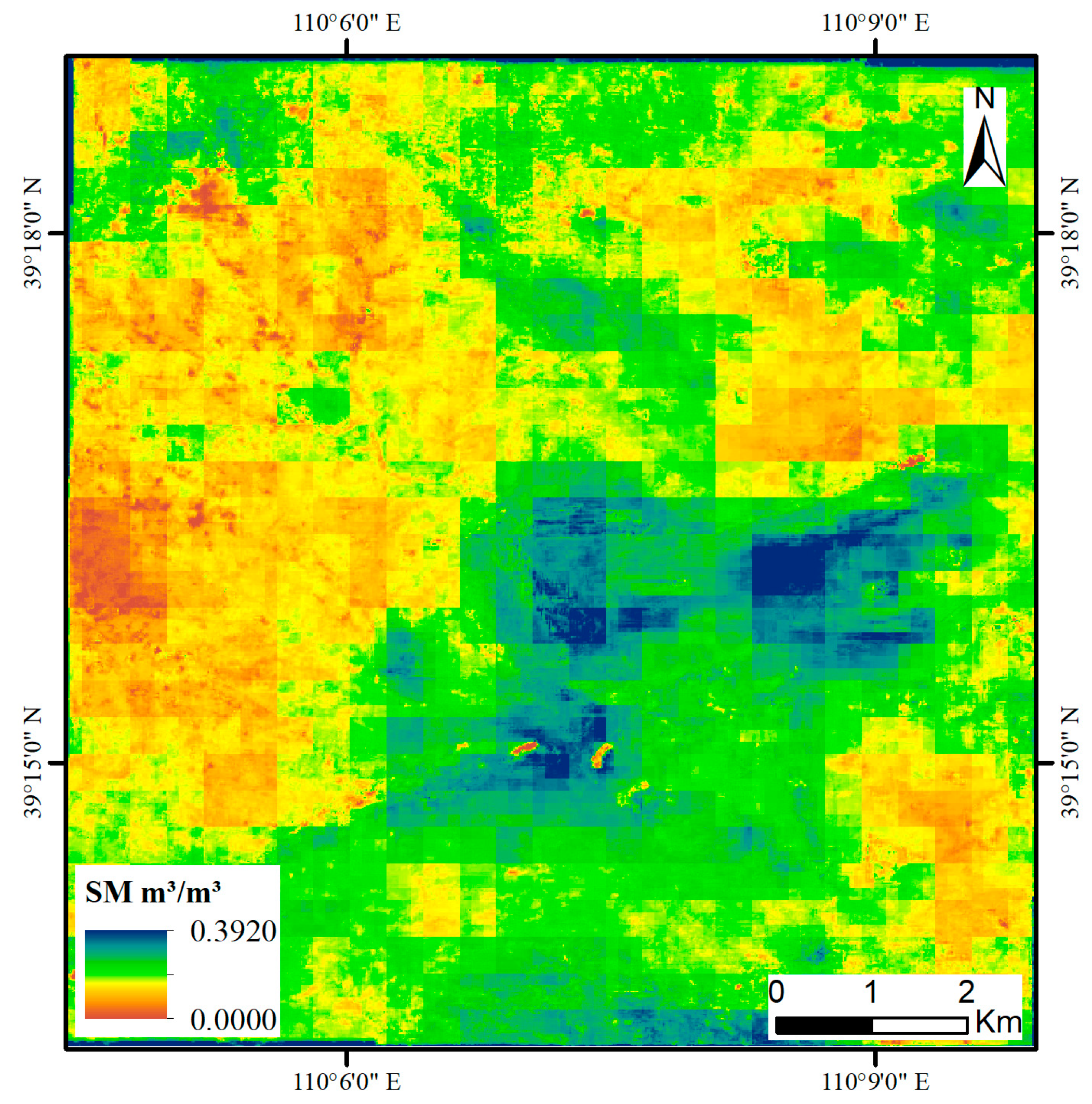
According to the above results, the downscaled SM derived from the 3 km SPL2SMAP_S SM product with the combination of reflectances + NDVI + DEM + slope as auxiliary data performs best, and the corresponding result is shown in Figure 7. It can be seen that the SM in the western part is lower than that in most other regions. There is an underground mine where the mining activities destroy the stability of the soil and reduce its resistance and recovery ability to environmental impact [70]. This result is consistent with the findings of Liu and Yue [70]. The SM in the south-central part is higher where there is an open-pit mine. It is probably because the excavation in the open-pit mine is carried out below the shallow aquifers, and water flows towards the mining works from the surrounding strata, which makes the surface SM higher than other places [71].
5. Discussion
5.1. Overview of the Downscaling Methodology
The SPL2SMAP_S V3 SM product is currently one of the highest spatial resolutions of SM products released worldwide and was available from 31 March 2015. It merges the SMAP radiometer brightness temperature data with a resolution of 40 km, and the Sentinel-1 radar backscatter data based on the SMAP Active–Passive algorithm. Based on the validation study over the SMAP Core Cal sites and the Sparse Network, the 3 km products’ unbiased RMSE is 0.05 m3/m3 [35]. Although the SPL2SMAP_S product is good, it does not satisfy the application requirements for ecological management in small-scale mine areas due to its coarse spatial resolution. In addition, the relationship between SM and impact factors such as vegetation in mining areas becomes unconventional due to the human exploitation of mineral resources [66]. The relationships in mining areas are more complex than that in general scenarios. For example, vegetation grows better in areas with a high SM under natural conditions, whereas in semiarid opencast mines, the destruction of shallow aquifers by coal mining results in a high SM and no vegetation growth. Under these contexts, we proposed a method to downscale the SPL2SMAP_S V3 products to a field-scale 10 m spatial resolution with the help of auxiliary datasets, and applied it in the Shangwan mine area, which contains both underground and open-pit mines. In addition, we took Sentinel-2 reflectances with a 10 m spatial resolution as the required input data and the other auxiliary data (e.g., vegetation and topographic information), which influences the SM distribution by affecting soil evapotranspiration and water dynamics, as optional input data. Finally, we designed the SM-RDNet network structure in order to obtain a more accurate SM. The SM-RDNet network solves the problem of computational resource consumption and gradient disappearance due to the increased number of layers in the network via the skip connection in the residual dense block. This effectively integrates low-level with high-level features and enhances the fitting ability.
5.2. Role of Geoinformation in Improving the Accuracy of the Downscaled SM
To derive accurate SM at small scale, NDVI, DEM and slope were taken as auxiliary data. According to Section 4.1 and Section 4.2, these factors do improve the downscaling accuracy to some extent compared with using reflectances alone. From the perspective of each data’s contribution to accuracy improvement, according to Table 2 and Table 3, NDVI provides the most improvement in accuracy in terms of RMSE while using only one auxiliary data, followed by DEM and slope. NDVI, representing the vegetation status, affect SM by soil evapotranspiration and the depth of penetration of microwaves into soil, while this is also an essential component in the method of optical remote sensing to inverse SM [51,72]. The DEM and slope are a quantitative description of the terrain. Topography affects SM distribution through soil–water dynamics, which can effectively improve the accuracy [47,48]. While using two auxiliary data, all combinations of auxiliary data do not improve the downscaling accuracy. Since the SM-RDNet, a black-box model, is agnostic in nature, we cannot provide a plausible explanation. Using all three auxiliary data performs best among all combinations, since there is a large improvement for all statistical metrics.
5.3. The Effect of Vegetation Cover on the Downscaling of SM
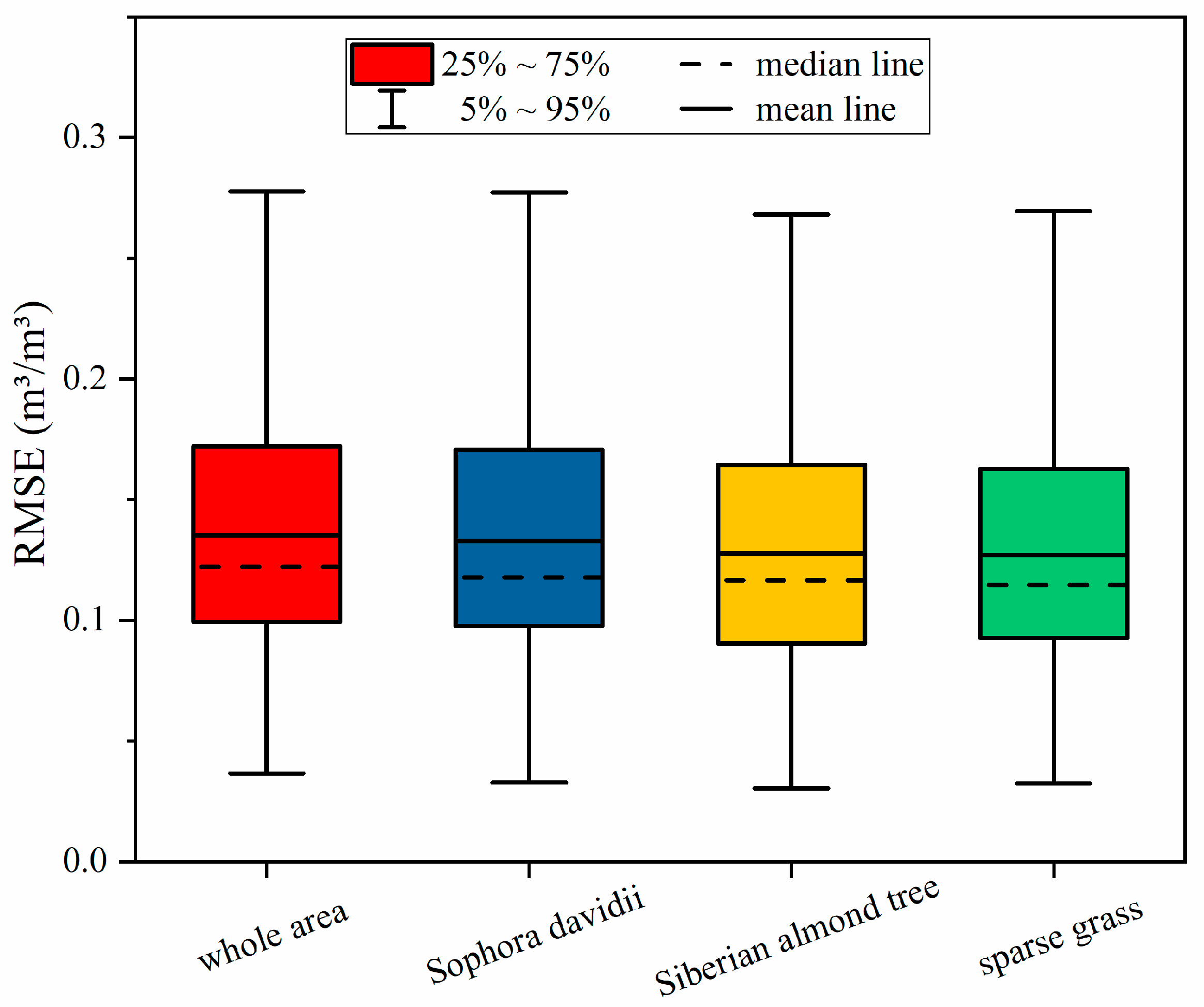
The study area is a gully area covered with multiple types of vegetation. Figure 8 shows full distribution of the downscaled SMs’ accuracy for the different data combinations in the whole area with mixed types of vegetation cover and the areas with a single type of vegetation cover, including Sophora davidii, Siberian almond tree and sparse grass. According to Figure 8, the downscaled SMs in the single type of vegetation cover have a slightly better performance than those in mixed types of vegetation cover. This is because the mixed types of vegetation cover have greater heterogeneity, where the relationship between the SM and vegetation is more complex and various. Since the main factor influencing SM is precipitation, rather than the vegetation [11], the difference for the downscaled SMs’ accuracy in each vegetation cover is relatively weak. Among all areas with a single type of vegetation cover, the SM downscaling performs best in sparse grass, so the proposed model performs better in grassland than in shrub-covered areas. This is partly because the grassland less attenuates microwaves compared with the shrub-covered area, which results in the original SM product being more accurate. In summary, the downscaled SMs in the single vegetation cover area have a better performance.
5.4. Comparison of Downscaled SM Derived from 1-Km and 3-Km SPL2SMAP_S SM Products
We compared the performance of downscaled SMs derived from the 1 km and 3 km SPL2SMAP_S SM products from two perspectives: statistical metric and the spatial distribution of the downscaled SM. According to Table 2 and Table 3, the statistical metrics of the downscaled SM derived from the 3 km product are overall better than that derived from the 1 km product. The reason could be that the 3 km SM products have a less spatial-scale mismatch and a better accuracy, which was indicated by Yee et al. [73] and van der Velde et al. [74]. The downscaled SM derived from the 3 km SPL2SMAP_S SM product performs best with the combination of all three auxiliary data, including NDVI, DEM and slope, and the RMSE is 0.0366 m3/m3. These results are consistent with Abowarda et al.’s [11] research, whose RMSE was 0.031–0.050 m3/m3 in the 30 m spatial resolution SM.
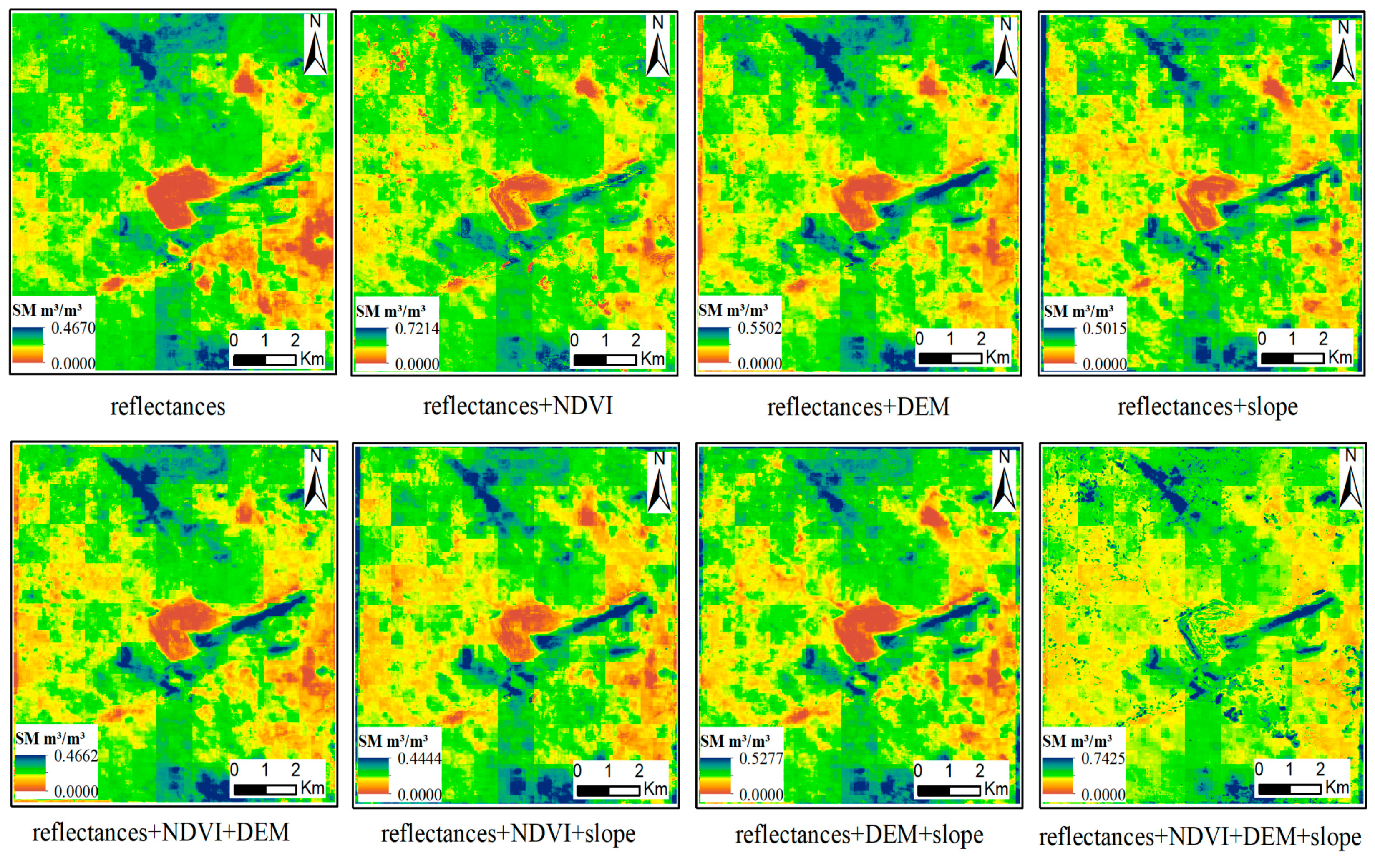
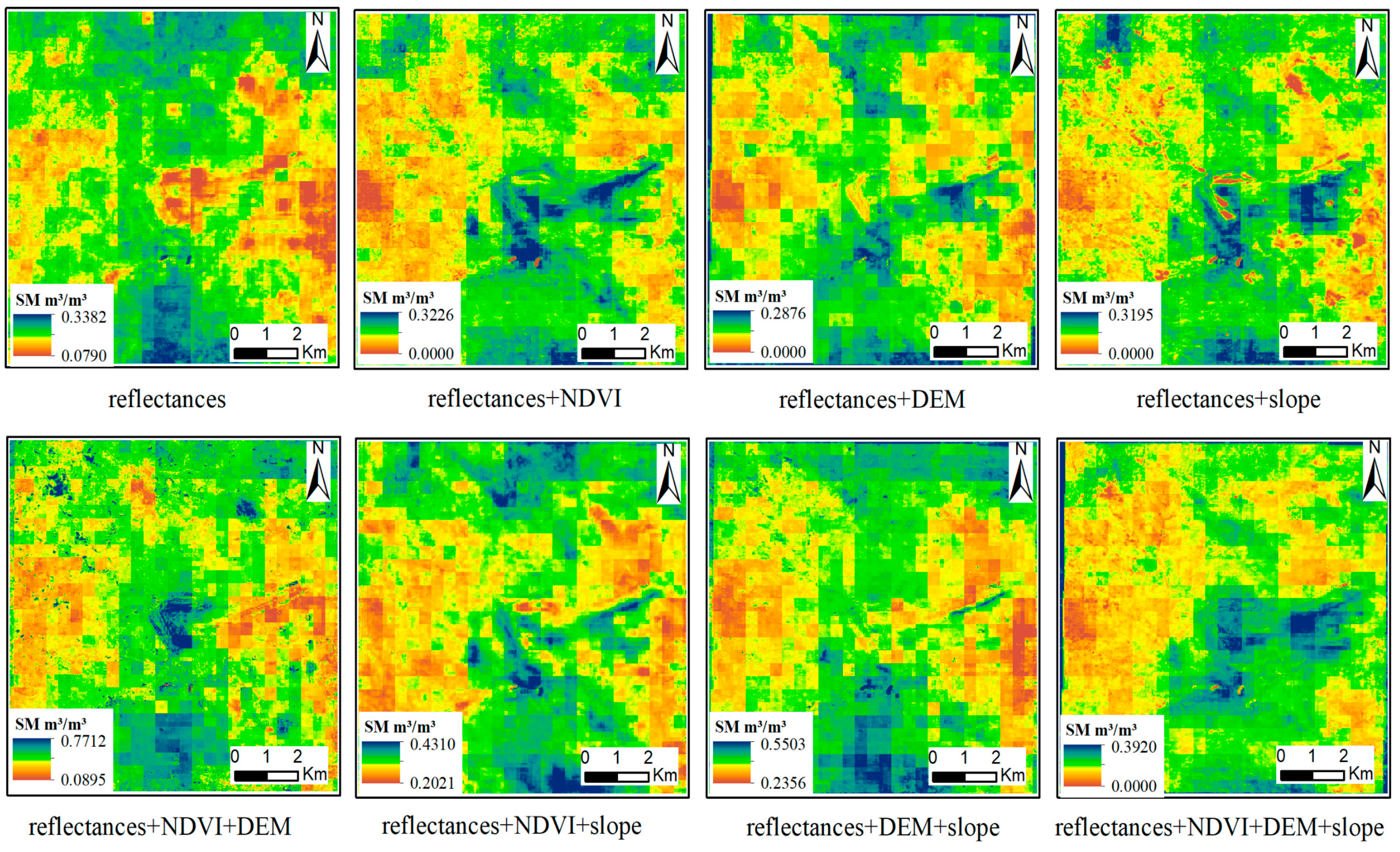
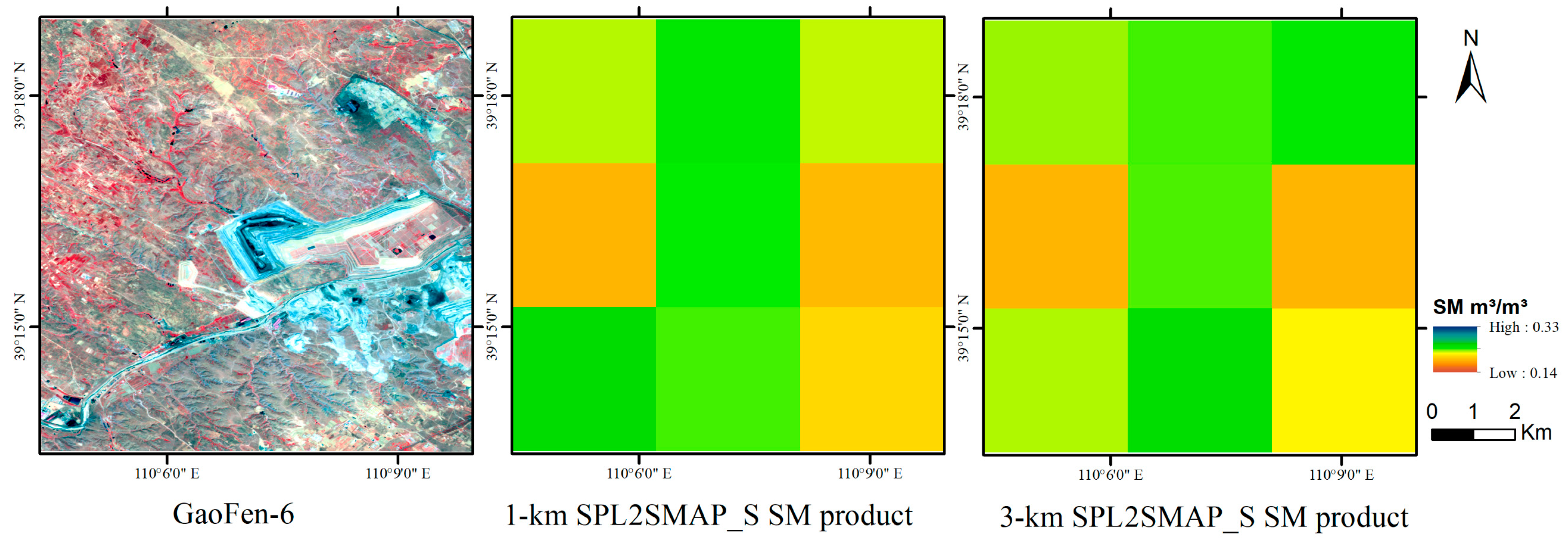
Figure 9 and Figure 10 show the spatial distribution of the downscaled SMs derived from the 1 km and 3 km SPL2SMAP_S SM products, respectively. Figure 11 shows the GaoFen-6 remotely sensed image with the 2 m spatial resolution and the SPL2SMAP_S SM products with the 1 km and 3 km spatial resolutions in the study area.
According to Figure 9 and Figure 10, the downscaled SM derived from the 1 km SPL2SMAP_S SM product have better spatial continuity than that derived from the 3 km product. Based on the GaoFen-6 remote sensing imagery (Figure 11), it is clear that the results obtained from the 1km SPL2SMAP_S SM product downscaling can better reflect the location and shape of the open-pit mine. However, the SM on open-pit mines is usually higher than on the surrounding unmined surface due to groundwater overflow from the destruction of aquifers by open-pit mining [71]. Therefore, most downscaled SMs derived from the 1 km resolution products shown in Figure 9 are inconsistent with the low SM in the central open pit relative to the surrounding area. In contrast, in the downscaled SMs derived from the 3 km resolution products (Figure 10), the SM is high in the central region and low in the western and eastern regions. What is more, the morphology of the area with the high SM values matches well with the open pit in Figure 11, particularly in the downscaled results using a combination of DEM + slope + NDVI as auxiliary data.
Based on the above analysis results, it can obtain the best performance by downscaling the SM from the 3 km product and using a combination of NDVI + DEM + slope as auxiliary data.
5.5. Comparison of Downscaled SM based on SM-RDNet and RF Model
We also compared the performance of the downscaled SMs based on the SM-RDNet model and the RF model, since previous studies have shown that the RF model performs well in downscaling for SM [43,59,75,76]. Since the combinations of reflectances + NDVI + DEM + slope derived from the 3 km SPL2SMAP_S SM products perform best (Section 5.4), we chose this combination for model comparison. The RMSE of the RF model is 0.1271 m3/m3 while the SM-RDNet is 0.0366 m3/m3. From a statistical point of view, the SM-RDNet model performs better than the RF model.
We compared the spatial distribution of the downscaled SMs based on the SM-RDNet and RF models. Figure 12 shows the downscaled SMs based on the SM-RDNet and RF models, respectively. According to Figure 12, it is clear that the downscaled SMs based on the SM-RDNet model are more continuous in space and show better spatial details compared to those based on the RF model. This is probably because the SM-RDNet uses a pixel block while conducting data fitting and makes full use of the information surrounding the central pixel, while the RF model uses a pixel-to-pixel strategy. It is worth noting that, for the open-pit mine, the RF model has not derived the right distribution of SM. In conclusion, the SM-RDNet model outperforms the RF model in the SM downscaling.
5.6. Analysis of Error Sources in Downscaling SM
Although the proposed method generates a good result and has the potential to be applied in mine ecological management and other fields, we still need to analyze its major error sources to ensure a scientific application. In this section, we discuss the potential sources of error from the perspective of the SPL2SMAP_S product, the in situ measurement, the downscaling process and the modeling process.
For SPL2SMAP_S products, there are three main sources of error, including the interpolation of SMAP brightness temperature data from 40 km to 9 km, the anthropogenic radio frequency interference and the high-resolution brightness temperature. Please refer to the user guide for SPL2SMAP_S [35] for detailed information. According to the validation study by Das et al. [35] over the SMAP Core Cal sites and the Sparse Network, the 3 km SPL2SMAP_S SM products have an ubRMSE of 0.05 m3/m3, while the 1 km SPL2SMAP_S SM products have not undergone validation.
For the in situ measurements, the TDR350 with a 3.8 cm probe used in our experiment measures the soil moisture at a depth of 3.8 cm from the surface. However, it is not clear how deep the SPL2SMAP_S SM products reflect the soil moisture, especially in the case of complex vegetation cover. Vegetation canopies attenuate the penetration of microwaves into the soil, especially for the C-band [51]. The diverse vegetation types in the study area vary in the attenuation of microwaves, so the soil depth that these SM products represent varies from vegetation type to vegetation type. Therefore, the mismatch between the in situ measurement and the microwave remotely sensed SM data is also a source of error.
For the downscaling process, several downscaling processes were performed in order to obtain the high-resolution SM. Although, in each, downscaling accuracy verification was conducted based on the truth SM values, errors were still inevitably introduced and accumulated.
In addition, there are some special mining-related human activities in the study area, such as coal mining and land reclamation. Different coal mining methods pose different effects on the surface SM. For example, underground mining could reduce the surface SM, since the mining activities destroy the stability of soil and reduce its resistance and recovery ability to environmental impacts. By contrast, open-pit mining could increase SM, since the removal of the topsoil and shallow aquifers above the coal seams can destroy the aquifers. In the reclaimed areas, the activities such as regular irrigation can contribute to an increase in SM. These human activities have resulted in much more complex relationships between SM and other factors than in natural scenarios, which is difficult to establish an accurate correlation model.
6. Conclusions
As the existing SM products fail to meet the requirements of fine ecological management in small-scale mining areas and represent the complex relationship between SM and related factors, a downscaling method based on deep learning is proposed. The key step of the method includes the SM-RDNet network structure and the downscaling strategy. Taking the Shangwan mine area as the study area, the experiments were carried out from several perspectives, including the type of original SM product, the combination of auxiliary datasets, the type of vegetation cover and comparison of models. Experimental results show that the proposed method can accurately obtain SM distributions at a spatial resolution of 10 m in mining areas. The key findings are as follows:
- (1)
- The 3 km SPL2SMAP_S SM product is a more reliable data source for SM downscaling, since its spatial scale matches better with the original observations of satellites. The RSME of the downscaled SM is 0.0366 m3/m3.
- (2)
- The combination of NDVI, DEM, slope and reflectances as auxiliary data obtains the highest downscaling accuracy due to the adequate information they contain.
- (3)
- The SM-RDNet performs better than the RF model, especially for mining areas with complex human activities. In addition, the downscaled SMs are better under a single vegetation cover, especially grassland.
In summary, we recommend downscaling the 3 km SPL2SMAP_S SM product to obtain fine-grained SM data for semiarid mining areas through the SM-RDNet network, combined with Sentinel-2, DEM, NDVI, and slope auxiliary data. The proposed method maximizes the potential of multisource data and deep learning algorithms in deriving fine-grained SM, which possess significant value to the managers of mining areas for fine ecological management and conservation in semiarid mining areas. Furthermore, with the fine-grained SM, how the mining effects SM in semiarid mining areas can be a subject of future research.
Author Contributions
Conceptualization, J.L. and C.Z. (Chengye Zhang); methodology, X.S.; software, J.X.; validation, X.L., H.W. and C.Z. (Caiyue Zhang); formal analysis, X.S.; investigation, X.L., H.W. and C.Z. (Caiyue Zhang).; writing—original draft preparation, X.S.; writing—review and editing, J.L.; visualization, X.S.; supervision, X.S.; funding acquisition, J.L. and C.Z. (Chengye Zhang). All authors have read and agreed to the published version of the manuscript.
Funding
This research was funded by the State Key Laboratory of Water Resource Protection and Utilization in Coal Mining (grant number GJNY-20-113-14), the National Natural Science Foundation of China (grant number 41901291, 42071314), the Fundamental Research Funds for the Central Universities (grant number 2022YJSDC21, 2022YQDC08, 2022JCCXDC04), Smart Group Entrepreneurship Program from Ningbo S&T Bureau (grant number 2021ZH1CXYD060013) and the Yueqi Young Scholars Program of China University of Mining and Technology-Beijing.
Institutional Review Board Statement
Not applicable.
Informed Consent Statement
Not applicable.
Data Availability Statement
The SPL2SMAP_S V3 can be downloaded from the website of the National Snow and Ice Data Center (NSIDC) (https://nsidc.org/data/SPL2SMAP_S, accessed on 17 June 2021). The Sentinel-2 images can be downloaded from the Google Earth Engine (GEE) (https://developers.google.com/earth-engine/datasets/, accessed on 17 June 2021). The topographic data downloaded from the website of National Aeronautics and Space Administration (NASA) EarthData (https://earthdata.nasa.gov/, accessed on 17 June 2021).
Acknowledgments
The authors thank Di Zhao from the China University of Mining and Technology-Beijing for her knowledge and advice on the hydrogeology of the mine area in this paper. The authors also thank Pixel Information Expert(PIE) Basic 6.0 software, provided by PIESAT International Information Technology Limited in Beijing, China, for supporting us with data processing, such as resample and resize.
Conflicts of Interest
The authors declare no conflict of interest.
References
- Saini, V.; Gupta, R.P.; Arora, M.K. Environmental impact studies in coalfields in India: A case study from Jharia coal-field. Renew. Sustain. Energy Rev. 2016, 53, 1222–1239. [Google Scholar] [CrossRef]
- Hasanuzzaman; Bhar, C.; Srivastava, V. Environmental capability: A Bradley–Terry model-based approach to examine the driving factors for sustainable coal-mining environment. Clean Technol. Environ. Policy 2018, 20, 995–1016. [Google Scholar] [CrossRef]
- Li, J.; Pei, Y.; Zhao, S.; Xiao, R.; Sang, X.; Zhang, C. A Review of Remote Sensing for Environmental Monitoring in China. Remote Sens. 2020, 12, 1130. [Google Scholar] [CrossRef] [Green Version]
- Giam, X.; Olden, J.D.; Simberloff, D. Impact of coal mining on stream biodiversity in the US and its regulatory implications. Nat. Sustain. 2018, 1, 176–183. [Google Scholar] [CrossRef]
- Manrique-Alba, À.; Ruiz-Yanetti, S.; Moutahir, H.; Novak, K.; de Luis, M.; Bellot, J. Soil moisture and its role in growth-climate relationships across an aridity gradient in semiarid Pinus halepensis forests. Sci. Total Environ. 2017, 574, 982–990. [Google Scholar] [CrossRef]
- Huang, Z.; Miao, H.-T.; Liu, Y.; Tian, F.-P.; He, H.; Shen, W.; López-Vicente, M.; Wu, G.-L. Soil water content and temporal stability in an arid area with natural and planted grasslands. Hydrol. Process. 2018, 32, 3784–3792. [Google Scholar] [CrossRef] [Green Version]
- Yang, M.J.; Wang, G.L.; Lazin, R.Y.; Shen, X.; Anagnostou, E. Impact of planting time soil moisture on cereal crop yield in the Upper Blue Nile Basin: A novel insight towards agricultural water management. Agric. Water Manag. 2021, 243, 106430. [Google Scholar] [CrossRef]
- Entekhabi, D.; Rodriguez-Iturbe, I.; Castelli, F. Mutual interaction of soil moisture state and atmospheric processes. J. Hydrol. 1996, 184, 3–17. [Google Scholar] [CrossRef]
- Seneviratne, S.I.; Corti, T.; Davin, E.L.; Hirschi, M.; Jaeger, E.B.; Lehner, I.; Orlowsky, B.; Teuling, A.J. Investigating soil moisture—Climate interactions in a changing climate: A review. Earth-Sci. Rev. 2010, 99, 125–161. [Google Scholar] [CrossRef]
- Sabaghy, S.; Walker, J.P.; Renzullo, L.J.; Jackson, T.J. Spatially enhanced passive microwave derived soil moisture: Capabilities and opportunities. Remote Sens. Environ. 2018, 209, 551–580. [Google Scholar] [CrossRef]
- Abowarda, A.S.; Bai, L.; Zhang, C.; Long, D.; Li, X.; Huang, Q.; Sun, Z. Generating surface soil moisture at 30 m spatial resolution using both data fusion and machine learning toward better water resources management at the field scale. Remote Sens. Environ. 2021, 255, 112301. [Google Scholar] [CrossRef]
- Zhang, C.Y.; Li, J.; Lei, S.G.; Yang, J.Z.; Yang, N. Progress and Prospect of the Quantitative Remote Sensing for Monitoring the Eco-environment in Mining Area. Met. Mine 2022, 3, 1–27. [Google Scholar]
- Friedl, M.A.; Davis, F.W. Sources of variation in radiometric surface temperature over a tallgrass prairie. Remote Sens. Environ. 1994, 48, 1–17. [Google Scholar] [CrossRef]
- Anderson, M.C.; Norman, J.M.; Mecikalski, J.R.; Otkin, J.A.; Kustas, W.P. A climatological study of evapotranspiration and moisture stress across the continental United States based on thermal remote sensing: 1. Model formulation. J. Geophys. Res. Earth Surf. 2007, 112, D10117. [Google Scholar] [CrossRef]
- Babaeian, E.; Sadeghi, M.; Franz, T.E.; Jones, S.; Tuller, M. Mapping soil moisture with the OPtical TRApezoid Model (OPTRAM) based on long-term MODIS observations. Remote Sens. Environ. 2018, 211, 425–440. [Google Scholar] [CrossRef]
- Entekhabi, D.; Njoku, E.G.; O’Neill, P.E.; Kellogg, K.H.; Crow, W.T.; Edelstein, W.N.; Entin, J.K.; Goodman, S.D.; Jackson, T.J.; Johnson, J.; et al. The Soil Moisture Active Passive (SMAP) Mission. Proc. IEEE 2010, 98, 704–716. [Google Scholar] [CrossRef]
- Wigneron, J.-P.; Li, X.; Frappart, F.; Fan, L.; Al-Yaari, A.; De Lannoy, G.; Liu, X.; Wang, M.; Le Masson, E.; Moisy, C. SMOS-IC data record of soil moisture and L-VOD: Historical development, applications and perspectives. Remote Sens. Environ. 2021, 254, 112238. [Google Scholar] [CrossRef]
- Ulaby, F.T.; Batlivala, P.P.; Dobson, M.C. Microwave Backscatter Dependence on Surface Roughness, Soil Moisture, and Soil Texture: Part I-Bare Soil. IEEE Trans. Geosci. Electron. 1978, 16, 286–295. [Google Scholar] [CrossRef]
- Ulaby, F.T.; Bradley, G.A.; Dobson, M.C. Microwave Backscatter Dependence on Surface Roughness, Soil Moisture, and Soil Texture: Part II-Vegetation-Covered Soil. IEEE Trans. Geosci. Electron. 1979, 17, 33–40. [Google Scholar] [CrossRef]
- Zribi, M.; Baghdadi, N.; Holah, N.; Fafin, O. New methodology for soil surface moisture estimation and its application to ENVISAT-ASAR multi-incidence data inversion. Remote Sens. Environ. 2005, 96, 485–496. [Google Scholar] [CrossRef]
- Zribi, M.; Andre, C.; Decharme, B. A Method for Soil Moisture Estimation in Western Africa Based on the ERS Scatterometer. IEEE Trans. Geosci. Remote Sens. 2008, 46, 438–448. [Google Scholar] [CrossRef]
- Njoku, E.G.; Jackson, T.J.; Lakshmi, V.; Chan, T.K.; Nghiem, S.J. Soil moisture retrieval from AMSR-E. IEEE Trans. Geosci. Remote Sens. 2003, 41, 215–229. [Google Scholar] [CrossRef]
- Geruo, A.; Velicogna, I.; Kimball, J.S.; Du, J.; Kim, Y.; Colliander, A.; Njoku, E. Satellite-observed changes in vegetation sensitivities to surface soil moisture and total water storage variations since the 2011 Texas drought. Environ. Res. Lett. 2017, 12, 054006. [Google Scholar] [CrossRef] [Green Version]
- Kerr, Y.H.; Waldteufel, P.; Richaume, P.; Wigneron, J.-P.; Ferrazzoli, P.; Mahmoodi, A.; Al Bitar, A.; Cabot, F.; Gruhier, C.; Juglea, S.E.; et al. The SMOS Soil Moisture Retrieval Algorithm. IEEE Trans. Geosci. Remote Sens. 2012, 50, 1384–1403. [Google Scholar] [CrossRef]
- Colliander, A.; Jackson, T.J.; Bindlish, R.; Chan, S.; Das, N.; Kim, S.B.; Cosh, M.H.; Dunbar, R.S.; Dang, L.; Pashaian, L.; et al. Validation of SMAP surface soil moisture products with core validation sites. Remote Sens. Environ. 2017, 191, 215–231. [Google Scholar] [CrossRef]
- Sabaghy, S.; Walker, J.P.; Renzullo, L.J.; Akbar, R.; Chan, S.; Chaubell, J.; Das, N.; Dunbar, R.S.; Entekhabi, D.; Gevaert, A.; et al. Comprehensive analysis of alternative downscaled soil moisture products. Remote Sens. Environ. 2020, 239, 111586. [Google Scholar] [CrossRef]
- Peng, J.; Loew, A.; Merlin, O.; Verhoest, N.E.C. A review of spatial downscaling of satellite remotely sensed soil moisture. Rev. Geophys. 2017, 55, 341–366. [Google Scholar] [CrossRef]
- Merlin, O.; Al Bitar, A.; Walker, J.; Kerr, Y. An improved algorithm for disaggregating microwave-derived soil moisture based on red, near-infrared and thermal-infrared data. Remote Sens. Environ. 2010, 114, 2305–2316. [Google Scholar] [CrossRef] [Green Version]
- Kim, J.; Hogue, T.S. Improving Spatial Soil Moisture Representation Through Integration of AMSR-E and MODIS Products. IEEE Trans. Geosci. Remote Sens. 2012, 50, 446–460. [Google Scholar] [CrossRef]
- Fang, B.; Lakshmi, V.; Bindlish, R.; Jackson, T.J. Downscaling of SMAP Soil Moisture Using Land Surface Temperature and Vegetation Data. Vadose Zone J. 2018, 17, 170198. [Google Scholar] [CrossRef] [Green Version]
- Merlin, O.; Escorihuela, M.J.; Mayoral, M.A.; Hagolle, O.; Al Bitar, A.; Kerr, Y. Self-calibrated evaporation-based disaggregation of SMOS soil moisture: An evaluation study at 3 km and 100 m resolution in Catalunya, Spain. Remote Sens. Environ. 2013, 130, 25–38. [Google Scholar] [CrossRef] [Green Version]
- Merlin, O.; Malbéteau, Y.; Notfi, Y.; Bacon, S.; Khabba, S.E.-R.S.; Jarlan, L. Performance Metrics for Soil Moisture Downscaling Methods: Application to DISPATCH Data in Central Morocco. Remote Sens. 2015, 7, 3783–3807. [Google Scholar] [CrossRef] [Green Version]
- Tian, J.; Deng, X.; Su, H. Intercomparison of two trapezoid-based soil moisture downscaling methods using three scaling factors. Int. J. Digit. Earth 2019, 12, 485–499. [Google Scholar] [CrossRef]
- Das, N.N.; Entekhabi, D.; Dunbar, R.S.; Chaubell, M.J.; Colliander, A.; Yueh, S.; Jagdhuber, T.; Chen, F.; Crow, W.; O’Neill, P.E.; et al. The SMAP and Copernicus Sentinel 1A/B microwave active-passive high resolution surface soil moisture product. Remote Sens. Environ. 2019, 233, 111380. [Google Scholar] [CrossRef]
- Das, N.; Entekhabi, D.; Dunbar, R.S.; Kim, S.; Yueh, S.; Colliander, A.; O’Neill, P.E.; Jackson, T.; Jagdhuber, T.; Chen, F.; et al. SMAP/Sentinel-1 L2 Radiometer/Radar 30-Second Scene 3-km EASE-Grid Soil Moisture, Version 3; NASA National Snow and Ice Data Center Distributed Active Archive Center: Boulder, CO, USA, 2020. [Google Scholar] [CrossRef]
- Zhan, X.W.; Houser, P.R.; Walker, J.P.; Crow, W.T. A method for retrieving high-resolution surface soil moisture from hydros L-band radiometer and Radar observations. IEEE Trans. Geosci. Remote Sens. 2006, 44, 1534–1544. [Google Scholar] [CrossRef]
- Wu, X.; Walker, J.P.; Rudiger, C.; Panciera, R.; Gao, Y. Medium-Resolution Soil Moisture Retrieval Using the Bayesian Merging Method. IEEE Trans. Geosci. Remote Sens. 2017, 55, 6482–6493. [Google Scholar] [CrossRef]
- Piles, M.; Entekhabi, D.; Camps, A. A Change Detection Algorithm for Retrieving High-Resolution Soil Moisture from SMAP Radar and Radiometer Observations. IEEE Trans. Geosci. Remote Sens. 2009, 47, 4125–4131. [Google Scholar] [CrossRef]
- Das, N.N.; Entekhabi, D.; Njoku, E.G. An Algorithm for Merging SMAP Radiometer and Radar Data for High-Resolution Soil-Moisture Retrieval. IEEE Trans. Geosci. Remote Sens. 2011, 49, 1504–1512. [Google Scholar] [CrossRef]
- Das, N.N.; Entekhabi, D.; Njoku, E.G.; Shi, J.J.C.; Johnson, J.T.; Colliander, A. Tests of the SMAP Combined Radar and Radiometer Algorithm Using Airborne Field Campaign Observations and Simulated Data. IEEE Trans. Geosci. Remote Sens. 2014, 52, 2018–2028. [Google Scholar] [CrossRef]
- Akbar, R.; Moghaddam, M. A Combined Active–Passive Soil Moisture Estimation Algorithm with Adaptive Regularization in Support of SMAP. IEEE Trans. Geosci. Remote Sens. 2015, 53, 3312–3324. [Google Scholar] [CrossRef]
- Wilson, D.J.; Western, A.W.; Grayson, R.B. A terrain and data-based method for generating the spatial distribution of soil moisture. Adv. Water Resour. 2005, 28, 43–54. [Google Scholar] [CrossRef]
- Yan, R.; Bai, J. A New Approach for Soil Moisture Downscaling in the Presence of Seasonal Difference. Remote Sens. 2020, 12, 2818. [Google Scholar] [CrossRef]
- Kim, G.; Barros, A.P. Space–time characterization of soil moisture from passive microwave remotely sensed imagery and ancillary data. Remote Sens. Environ. 2002, 81, 393–403. [Google Scholar] [CrossRef]
- Vereecken, H.; Huisman, J.A.; Bogena, H.; Vanderborght, J.; Vrugt, J.A.; Hopmans, J. On the value of soil moisture measurements in vadose zone hydrology: A review. Water Resour. Res. 2008, 44, W00D06. [Google Scholar] [CrossRef] [Green Version]
- Crow, W.T.; Berg, A.A.; Cosh, M.H.; Loew, A.; Mohanty, B.P.; Panciera, R.; de Rosnay, P.; Ryu, D.; Walker, J.P. Upscaling sparse ground-based soil moisture observations for the validation of coarse-resolution satellite soil moisture products. Rev. Geophys. 2012, 50, RG2002. [Google Scholar] [CrossRef] [Green Version]
- Cowley, G.S.; Niemann, J.D.; Green, T.R.; Seyfried, M.S.; Jones, A.S.; Grazaitis, P.J. Impacts of precipitation and potential evapotranspiration patterns on downscaling soil moisture in regions with large topographic relief. Water Resour. Res. 2017, 53, 1553–1574. [Google Scholar] [CrossRef]
- Yan, H.B.; Zhou, G.Q.; Yang, F.F.; Lu, X.J. DEM correction to the TVDI method on drought monitoring in karst areas. Int. J. Remote Sens. 2019, 40, 2166–2189. [Google Scholar] [CrossRef]
- El Hajj, M.; Baghdadi, N.; Zribi, M.; Bazzi, H. Synergic Use of Sentinel-1 and Sentinel-2 Images for Operational Soil Moisture Mapping at High Spatial Resolution Over Agricultural Areas. Remote Sens. 2017, 9, 1292. [Google Scholar] [CrossRef] [Green Version]
- Deshon, J.P.; Niemann, J.D.; Green, T.R.; Jones, A.; Grazaitis, P.J. Stochastic analysis and probabilistic downscaling of soil moisture in small catchments. J. Hydrol. 2020, 585, 124711. [Google Scholar] [CrossRef]
- Babaeian, E.; Sadeghi, M.; Jones, S.B.; Montzka, C.; Vereecken, H.; Tuller, M. Ground, Proximal, and Satellite Remote Sensing of Soil Moisture. Rev. Geophys. 2019, 57, 530–616. [Google Scholar] [CrossRef] [Green Version]
- Shi, H.; Fu, X.; Chen, J.; Wang, G.; Li, T. Spatial distribution of monthly potential evaporation over mountainous regions: Case of the Lhasa River basin, China. Hydrol. Sci. J. 2014, 59, 1856–1871. [Google Scholar] [CrossRef]
- Ranney, K.J.; Niemann, J.D.; Lehman, B.M.; Green, T.R.; Jones, A.S. A method to downscale soil moisture to fine resolutions using topographic, vegetation, and soil data. Adv. Water Resour. 2015, 76, 81–96. [Google Scholar] [CrossRef] [Green Version]
- Chai, S.-S.; Walker, J.P.; Makarynskyy, O.; Kuhn, M.; Veenendaal, B.; West, G. Use of Soil Moisture Variability in Artificial Neural Network Retrieval of Soil Moisture. Remote Sens. 2009, 2, 166–190. [Google Scholar] [CrossRef] [Green Version]
- Zhao, W.; Sanchez, N.; Lu, H.; Li, A. A spatial downscaling approach for the SMAP passive surface soil moisture product using random forest regression. J. Hydrol. 2018, 563, 1009–1024. [Google Scholar] [CrossRef]
- Wei, Z.S.; Meng, Y.Z.; Zhang, W.; Peng, J.; Meng, L.K. Downscaling SMAP soil moisture estimation with gradient boosting decision tree regression over the Tibetan Plateau. Remote Sens. Environ. 2019, 225, 30–44. [Google Scholar] [CrossRef]
- Yuan, Q.; Shen, H.F.; Li, T.W.; Li, Z.W.; Li, S.W.; Jiang, Y.; Xu, H.Z.; Tan, W.W.; Yang, Q.W.; Wang, J.; et al. Deep learning in environmental remote sensing: Achievements and challenges. Remote Sens. Environ. 2020, 241, 111716. [Google Scholar] [CrossRef]
- Senanayake, I.P.; Yeo, I.-Y.; Walker, J.P.; Willgoose, G.R. Estimating catchment scale soil moisture at a high spatial resolution: Integrating remote sensing and machine learning. Sci. Total Environ. 2021, 776, 145924. [Google Scholar] [CrossRef]
- Liu, Y.; Jing, W.; Wang, Q.; Xia, X. Generating high-resolution daily soil moisture by using spatial downscaling techniques: A comparison of six machine learning algorithms. Adv. Water Resour. 2020, 141, 103601. [Google Scholar] [CrossRef]
- LeCun, Y.; Bengio, Y.; Hinton, G. Deep learning. Nature 2015, 521, 436–444. [Google Scholar] [CrossRef]
- Xu, W.; Zhang, Z.; Long, Z.; Qin, Q. Downscaling SMAP Soil Moisture Products with Convolutional Neural Network. IEEE J. Sel. Top. Appl. Earth Obs. Remote Sens. 2021, 14, 4051–4062. [Google Scholar] [CrossRef]
- Bai, L.; Long, D.; Yan, L. Estimation of Surface Soil Moisture with Downscaled Land Surface Temperatures Using a Data Fusion Approach for Heterogeneous Agricultural Land. Water Resour. Res. 2019, 55, 1105–1128. [Google Scholar] [CrossRef]
- Vergopolan, N.; Chaney, N.W.; Beck, H.E.; Pan, M.; Sheffield, J.; Chan, S.; Wood, E.F. Combining hyper-resolution land surface modeling with SMAP brightness temperatures to obtain 30-m soil moisture estimates. Remote Sens. Environ. 2020, 242, 111740. [Google Scholar] [CrossRef]
- Zhang, D.S.; Fan, G.W.; Liu, Y.D.; Ma, L.Q. Field trials of aquifer protection in longwall mining of shallow coal seams in China. Int. J. Rock Mech. Min. Sci. 2010, 47, 908–914. [Google Scholar] [CrossRef]
- Xiao, W.; Zhang, W.; Ye, Y.; Lv, X.; Yang, W. Is underground coal mining causing land degradation and significantly damaging ecosystems in semi-arid areas? A study from an Ecological Capital perspective. Land Degrad. Dev. 2020, 31, 1969–1989. [Google Scholar] [CrossRef]
- Li, J.; Peng, S.; Zhang, C.; Yang, F.; Sang, X. Quantitative remote sensing-based monitoring and evaluation of the ecological environment in mining areas: Technology framework and application. J. Min. Sci. Technol. 2022, 7, 9–25. [Google Scholar] [CrossRef]
- Rogers, D.J.; Randolph, S.E. Mortality rates and population density of tsetse flies correlated with satellite imagery. Nature 1991, 351, 739–741. [Google Scholar] [CrossRef]
- Zhang, Y.; Tian, Y.; Kong, Y.; Zhong, B.; Fu, Y. Residual Dense Network for Image Super-Resolution. In Proceedings of the 2018 IEEE/CVF Conference on Computer Vision and Pattern Recognition, Salt Lake City, UT, USA, 18–23 June 2018; pp. 2472–2481. [Google Scholar] [CrossRef] [Green Version]
- Gruber, A.; De Lannoy, G.; Albergel, C.; Al-Yaari, A.; Brocca, L.; Calvet, J.-C.; Colliander, A.; Cosh, M.; Crow, W.; Dorigo, W.; et al. Validation practices for satellite soil moisture retrievals: What are (the) errors? Remote Sens. Environ. 2020, 244, 111806. [Google Scholar] [CrossRef]
- Liu, Y.; Yue, H. Remote Sensing Monitoring of Soil Moisture in the Daliuta Coal Mine Based on SPOT 5/6 and Worldview-2. Open Geosci. 2019, 11, 866–876. [Google Scholar] [CrossRef]
- Bahrami, S.; Ardejani, F.D.; Baafi, E. Application of artificial neural network coupled with genetic algorithm and simulated annealing to solve groundwater inflow problem to an advancing open pit mine. J. Hydrol. 2016, 536, 471–484. [Google Scholar] [CrossRef] [Green Version]
- Sadeghi, M.; Babaeian, E.; Tuller, M.; Jones, S.B. The optical trapezoid model: A novel approach to remote sensing of soil moisture applied to Sentinel-2 and Landsat-8 observations. Remote Sens. Environ. 2017, 198, 52–68. [Google Scholar] [CrossRef] [Green Version]
- Yee, M.S.; Walker, J.P.; Monerris, A.; Rüdiger, C.; Jackson, T.J. On the identification of representative in situ soil moisture monitoring stations for the validation of SMAP soil moisture products in Australia. J. Hydrol. 2016, 537, 367–381. [Google Scholar] [CrossRef]
- van der Velde, R.; Salama, M.S.; van Helvoirt, M.D.; Su, Z.; Ma, Y. Decomposition of Uncertainties between Coarse MM5–Noah-Simulated and Fine ASAR-Retrieved Soil Moisture over Central Tibet. J. Hydrometeorol. 2012, 13, 1925–1938. [Google Scholar] [CrossRef]
- Long, D.; Bai, L.L.; Yan, L.; Zhang, C.J.; Yang, W.T.; Lei, H.M.; Quan, J.L.; Meng, X.Y.; Shi, C.X. Generation of spatially complete and daily continuous surface soil moisture of high spatial resolution. Remote Sens. Environ. 2019, 233, 111364. [Google Scholar] [CrossRef]
- Peng, J.; Albergel, C.; Balenzano, A.; Brocca, L.; Cartus, O.; Cosh, M.H.; Crow, W.T.; Dabrowska-Zielinska, K.; Dadson, S.; Davidson, M.W.; et al. A roadmap for high-resolution satellite soil moisture applications–confronting product characteristics with user requirements. Remote Sens. Environ. 2020, 252, 112162. [Google Scholar] [CrossRef]
Figure 1.
Location of the study area.

Figure 2.
A sample point in the field survey.

Figure 3.
Spatial distribution of the in situ measurements data.

Figure 4.
Network structure of SM-RDNet.

Figure 5.
Flow chart of SM downscaling.

Figure 6.
The pictures for (a) Sophora davidii, (b) Siberian almond tree and (c) sparse grass in the study area.
Figure 6.
The pictures for (a) Sophora davidii, (b) Siberian almond tree and (c) sparse grass in the study area.

Figure 7.
Spatial distribution of downscaled SM from 3 km SPL2SMAP_S in the study area using all auxiliary data.
Figure 7.
Spatial distribution of downscaled SM from 3 km SPL2SMAP_S in the study area using all auxiliary data.

Figure 8.
The boxplot of downscaled SMs’ accuracy in the whole area and the single vegetation covers.
Figure 8.
The boxplot of downscaled SMs’ accuracy in the whole area and the single vegetation covers.

Figure 9.
The downscaled SMs derived from 1 km SPL2SMAP_S SM products on 14 May 2021.

Figure 10.
The downscaled SMs derived from 3 km SPL2SMAP_S SM products on 14 May 2021.

Figure 11.
The GaoFen-6 remotely sensed image and the SPL2SMAP_S SM products in the study area.

Figure 12.
The downscaled SMs based on the (a) SM-RDNet and (b) RF models.


Table 1.
The wavelength bands used in the Sentinel-2 data.
| Band Name | Resolution | Description | Band Name | Resolution | Description |
|---|---|---|---|---|---|
| B2 | 10 m | Blue | B3 | 10 m | Green |
| B4 | 10 m | Red | B5 | 20 m | Red Edge 1 |
| B6 | 20 m | Red Edge 2 | B7 | 20 m | Red Edge 3 |
| B8 | 10 m | NIR | B8A | 20 m | Red Edge 4 |
| B11 | 20 m | SWIR 1 | B12 | 20 m | SWIR 2 |
Table 2.
RMSEs of the downscaled SMs derived from 1 km SPL2SMAP_S SM product (m3/m3).
| Input Data Sets | Whole Area (n 1 = 54) | Sophora Davidii (n 1 = 9) | Siberian Almond Tree (n 1 = 14) | Sparse Grass (n 1 = 13) |
|---|---|---|---|---|
| reflectances | 0.1932 | 0.1911 | 0.1860 | 0.1841 |
| reflectances + NDVI | 0.0944 | 0.0912 | 0.0867 | 0.0882 |
| reflectances + DEM | 0.1121 | 0.1105 | 0.1043 | 0.1063 |
| reflectances + slope | 0.1207 | 0.1156 | 0.1152 | 0.1139 |
| reflectances + NDVI + DEM | 0.1236 | 0.1201 | 0.1179 | 0.1153 |
| reflectances + NDVI + slope | 0.1341 | 0.1324 | 0.1271 | 0.1255 |
| reflectances + NDVI + slope | 0.1281 | 0.1250 | 0.1229 | 0.1195 |
| reflectances + NDVI + DEM + slope | 0.1065 | 0.1040 | 0.0995 | 0.0979 |
1 n is the number of sample points.
Table 3.
RMSEs of the downscaled SMs derived from 3 km SPL2SMAP_S SM product (m3/m3).
| Input Data Sets | Whole Area (n 1 = 54) | Sophora Davidii (n 1 = 9) | Siberian Almond Tree (n 1 = 14) | Sparse Grass (n 1 = 13) |
|---|---|---|---|---|
| reflectances | 0.1510 | 0.1504 | 0.1426 | 0.1416 |
| reflectances + NDVI | 0.0509 | 0.0483 | 0.0437 | 0.0396 |
| reflectances + DEM | 0.0774 | 0.0761 | 0.0676 | 0.0675 |
| reflectances + slope | 0.1046 | 0.1053 | 0.0943 | 0.0969 |
| reflectances + NDVI + DEM | 0.2776 | 0.2772 | 0.2681 | 0.2696 |
| reflectances + NDVI + slope | 0.2189 | 0.2158 | 0.2115 | 0.2101 |
| reflectances + DEM + slope | 0.2331 | 0.2307 | 0.2263 | 0.2238 |
| reflectances + NDVI + DEM + slope | 0.0366 | 0.0328 | 0.0305 | 0.0324 |
1 n is the number of sample points.
Publisher’s Note: MDPI stays neutral with regard to jurisdictional claims in published maps and institutional affiliations. |
© 2022 by the authors. Licensee MDPI, Basel, Switzerland. This article is an open access article distributed under the terms and conditions of the Creative Commons Attribution (CC BY) license (https://creativecommons.org/licenses/by/4.0/).
Share and Cite
MDPI and ACS Style
Sang, X.; Li, J.; Zhang, C.; Xing, J.; Liu, X.; Wang, H.; Zhang, C. Downscaling Microwave Soil Moisture Products with SM-RDNet for Semiarid Mining Areas. Water 2022, 14, 1792. https://doi.org/10.3390/w14111792
AMA Style
Sang X, Li J, Zhang C, Xing J, Liu X, Wang H, Zhang C. Downscaling Microwave Soil Moisture Products with SM-RDNet for Semiarid Mining Areas. Water. 2022; 14(11):1792. https://doi.org/10.3390/w14111792
Chicago/Turabian StyleSang, Xiao, Jun Li, Chengye Zhang, Jianghe Xing, Xinhua Liu, Hongpeng Wang, and Caiyue Zhang. 2022. "Downscaling Microwave Soil Moisture Products with SM-RDNet for Semiarid Mining Areas" Water 14, no. 11: 1792. https://doi.org/10.3390/w14111792
Note that from the first issue of 2016, this journal uses article numbers instead of page numbers. See further details here.