
Appraisal of Socio-Technical Water Loss Control Strategies Using Cost-Benefit Analysis in a Water Supply Network


1
Department of Civil Engineering Science, University of Johannesburg, Auckland Park, P.O. Box 524, Johannesburg 2006, South Africa
2
Directorate of Engineering the Future, School of Science, Engineering and Environment, The University of Salford, Newton Building, Greater Manchester M5 4WT, UK
3
Department of Town Planning, Engineering Networks and Systems, South Ural State University, 76, Lenin Prospekt, 454080 Chelyabinsk, Russia
4
Department of Civil Engineering, Water Sisulu University, Old Berlin Road, Fort Jackson, P.O. Box 1421, East London 5200, South Africa
*
Author to whom correspondence should be addressed.
Water 2022, 14(11), 1789; https://doi.org/10.3390/w14111789
Submission received: 21 April 2022
/
Revised: 20 May 2022
/
Accepted: 27 May 2022
/
Published: 2 June 2022
(This article belongs to the Section Urban Water Management)
Abstract
:The authors conducted a socio-technical cost–benefit analysis (CBA) in Alexandra Township (Alex for short) by combining three water loss control investment strategies: (i) pipeline and infrastructure upgrades, (ii) repair and maintenance, and (iii) socio-domestic retrofitting capital. The researchers performed the CBA using sensitivity analysis methodologies such as marginal cost of capital (MCC), weighted average cost of capital (WACC), coefficient of variance (CV), the net present value (NPV) ratio, and cumulative and total cost methods. The findings for socio-domestic retrofitting capital investment showed that at an average investment cost of USD 5735 per household, consumption was reduced from 1369.4 m3/year to 301.99 m3/year, whereas a projected water savings average of 521.05 m3/household/year was achieved. The results show that the cumulative cost of water losses equaled USD 43.9 million per year, and that, if the water loss trend continues beyond the year 2026, almost 100% of the system input volume (SIV) will be non-revenue water (NRW) in the water balance. Using the MCC method, the integrated results for the socio-technical strategy showed that the economic level of leakage (ELL) was achieved at a WACC of 16.2, a CV of 0.66, and an NPV ratio or net capital risk of 0.246. This study demonstrates that the socio-technical approach is a viable alternative for water loss control and may be adopted in various parts of the world.
1. Introduction
Fresh water, a limited resource, continues to be depleted due to high consumption and infrastructural losses [1,2]. As an economic good, reducing water losses tops the priority list of the majority of water utilities globally [3,4,5]. According to the United Nations [1], over 126 billion cubic meters of water, equivalent to USD 39 billion, are recorded as non-revenue water (NRW) annually around the world. Some of the factors that contribute to high water losses in developing countries are as follows: increasing migration into urban areas, resulting in high water demands; socio-economic factors, resulting in non-payment for water usage; poor infrastructure management; metering inaccuracies; sub-standard repair and maintenance strategies; financial challenges; ageing infrastructure; water theft; and poor governance [5,6,7,8]. However, curbing water losses comes at a high cost and requires long-term capital investments [5,7,9,10,11,12]. Water utilities around the world have always engineered solutions and strategies to evaluate, manage, and monitor water losses. However, the complex existing gaps make applying any of the solutions impractical due to the cost implications [9,12,13].
According to the aforementioned literature, as a result of the associated water loss control costs that water utilities in some part of the world face, there is a contradictory outlook with regard to the factors contributing to water loss versus the available water loss reduction strategies [8,9,10,11,12,13]. However, despite the above assertion, there is some consensus in some research publications on water losses that indicates that the application of a cost–benefit analysis in water loss control is amongst the best methods when deciding which water loss capital investment option to select [14,15,16,17,18,19,20].
In practice, cost–benefit analyses provide various financial indicators that are useful in capital investment decision-making for water loss management [19,20,21]. According to Heryanto et al. [21], water loss control strategies that are CBA-driven go as far back as the mid-1990s in England and Wales as a sub-concept of the economic level of leakages (ELL). The ELL is a cost–benefit approach that focuses on the total cost method (TCM), where active leak control (ALC) frequencies are measured and calculated per unit cost of water [21]. The baseline data needed to measure the TCM comprise the annual total cost of water versus the annual cost required to reduce water losses [21,22]. The ELL, as a sub-component method of the TCM, has, however, evolved over time, whereby it has integrated leakage flowrates (LFRs) of reported and unreported bursts in water distribution systems [23].
In the early 2000s, the total cost method (TCM) was reinterpreted as the total leakage flow rate (TLFR) method, where the cost of water per unit rate multiplied by the volume of water lost per component measure was used to determine the total cost of water [23,24,25]. The total leakage flow rate (TLFR) uses average leak duration (ALD) for reported bursts, unreported bursts, and leaking connections. This method measures them against average flows per unit measure multiplied by the number of reported leakages [25,26]. In practice, the TLFR is useful when computing the total cost of water and its cumulative cost for a specific distribution system [12,24,26].
Another practical CBA method is called the marginal cost of capital (MCC) method, which is the cumulative investment of the capital cost of total leakages per year divided by the total volume of water loss recorded for the same period [21,22]. The MCC is also used to measure the ELL, in which the cumulative cost method graph intersects with the cumulative benefit of capital investment [19,20,21,22]. Furthermore, other CBA components in practice are the concept of the time value of money (TVM), in which financial indicators such as net present value (NPV) and future value (FV) have been applied with great success around the world [18,19,27]. The TVM financial indicators integrate the projected interests on investment and corresponding future returns [19,20]. The two sub-methods of NPV and FV are used to calculate the value of investments over a time period. For instance, the NPV is used in capital budgeting to analyze the profitability of a projected investment or project [18,27]. The NPV and FV methods use capital investment in water loss reduction, and compound that over a particular period [13,19,27]. This is performed to determine the FV of the investment and its NPV ratio outlook when discounting the investment backwards [28].
Furthermore, other CBA efficiency indicators used in practice are risk-orientated methods such as the weighted average cost of capital (WACC) and the coefficient of variance (CV). By definition, the WACC is the comprehensive percentage ratio of the total cumulative cost of a project investment against its individual sub-component contributions. WACC is commonly referred to as the firm’s total capital cost and its risk is dictated mostly by external markets [29,30,31]. Researchers compute the WACC by multiplying the sub-total cost of each capital source in the investment (debt and equity) by its corresponding market weight value of compounding interests, and then adding the products of each capital source together to determine the total WACC [19,20,31]. The coefficient of variance (CV), on the other hand, is a relative measure of risk variation. The CV is actually a ratio of the standard deviation (SD) of a specific distribution to its mean, and it measures the net risk and return ratio on capital investment for any project [19,32].
Therefore, other prior studies have proven that the above list of CBA methods is not exhaustive as it is highly improbable that all CBA indicators can be analyzed in a single study [18,19,20,21,30,31,32]. In order to carry out a cost–benefit analysis of water loss control strategies currently in practice, our team selected Alexandra Township in Johannesburg as the study area [12,33,34,35]. The study was motivated by practically observing the prevailing socio-economic conditions in Alexandra, as well as reviewing other internal reports (some of them were notes of personal communications) about water losses in Alexandra [35]. In 2016, Alexandra Township recorded 87.02% of the total system input volume as actual non-revenue water, which is equal to a value of USD 49.882 million [35]. As a result of its dense population, complex socio-economic conditions, and deteriorating water infrastructure [12,35], Alexandra Township represents an appropriate real-world scenario in which to conduct a cost–benefit analysis on water loss control. In comparison to other research studies, our motivation was to reduce water losses in a cost-effective manner in a water distribution network, which can guarantee sustainable water security and provision [35,36,37,38,39]. Moreover, no previous water loss control studies have been conducted in South Africa or in other similar countries with a focus on a socio-economic area like the Alexandra township. In this study, we aimed to close the knowledge gap in urban water management regarding the reduction of water losses.
2. Materials and Methods
2.1. Overview of Methodologies
The methodology used to achieve the study objective involved a combination of activities such as a desktop study, scientific mathematical procedures, financial performance indicator methods, and on-site visual data collection and subsequent analysis. The authors collected and analyzed data in the following categories: (i) scientific and hydraulic data flow logging; (ii) customer consumption data; (iii) repair and maintenance data and the corresponding capital investment costs; (iv) capital investment data on new pipeline upgrades; and (v) capital investment on socio-domestic retrofitting data. The authors also performed a sensitivity analysis procedure on all data to determine the CBA indexes and ELL using the MCC method, WACC, NPV ratio methods, coefficient of variance (CV), and the cumulative total cost method. All available data findings were integrated in this study and are presented in tables and figures in the following sections.
2.2. Research Instrumentation Setup
Primary, the data analyzed and presented in this paper were collected between September 2020 and August 2021. The authors conducted visual field data collection on customer meters and gathered secondary data from several internal documents, such as technical planning reports, annual budgetary plans, existing water distribution system drawings, capital and operational financial expenditure reports, and annual performance audit reports. Furthermore, the authors performed an in-depth hydraulic flow analysis using the Water Distribution and System Optimization (WADISO) (GLS Software (PTY) Ltd., Pretoria, South Africa) tool, which is a hydraulic modelling software (similar to EPANET 2.2 (US EPA Research, Durham, NC, USA) [7,12]. The WADISO software helped the authors to analyze the existing age of the infrastructure and remaining useful life [12]. The researchers used WADISO for system synchronization and the identification of the six district metered areas (DMA) in which bulk flow logging was conducted using ultra-sonic flow pressure devices for a period of 15 days. These data were used for the annual interpolation of total system input volume (SIV), as presented in the following section of this paper.
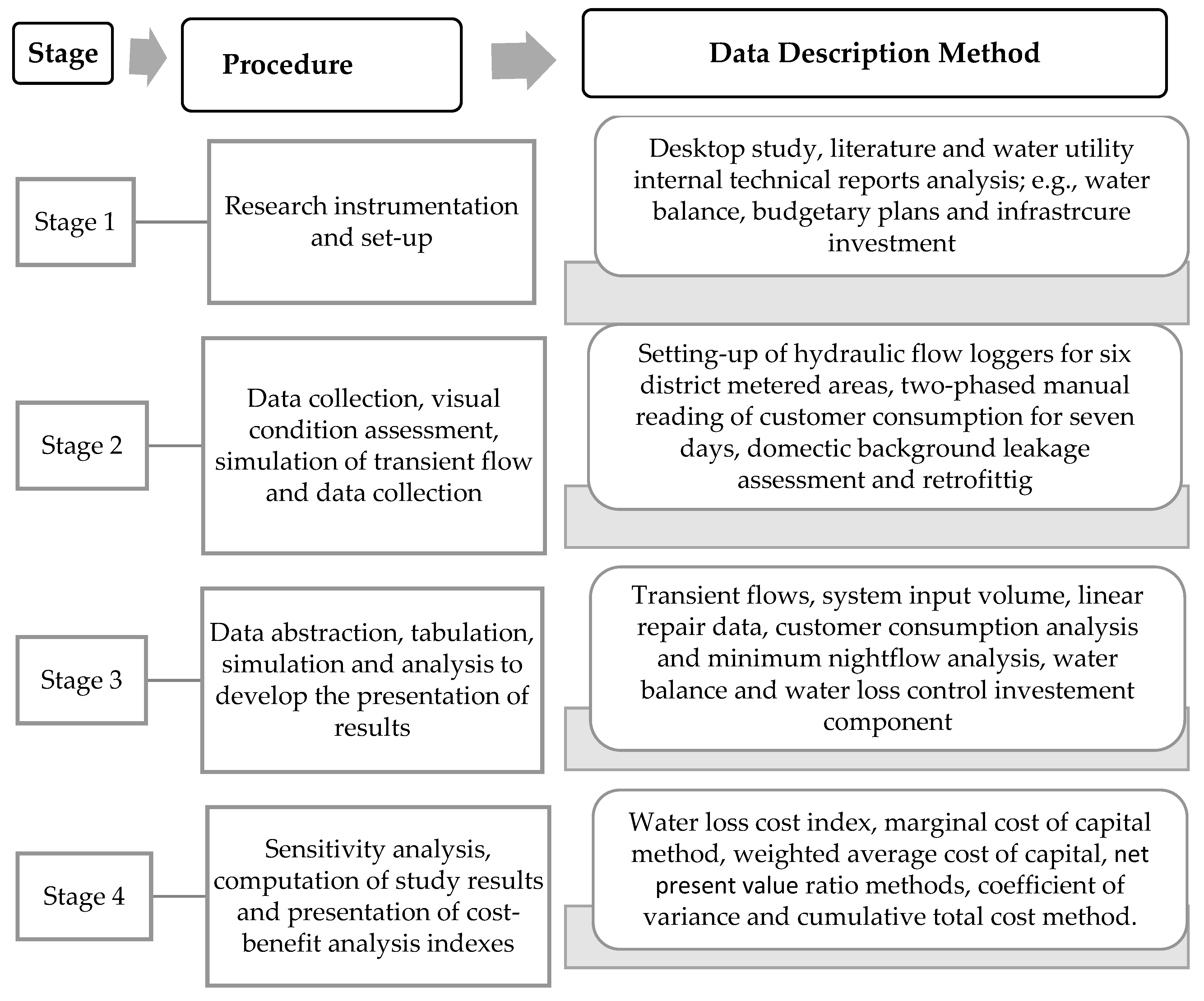
Additionally, relevant information was collected, which included the yearly International Water Association (IWA) water balance, costs related to water loss reduction, the total cost of production, water tariffs, the activity procedure for active leakage control, and different domestic background leakage trends. The data from the water utilities were only available from 2015 to 2019, which was the period used for the analysis. Figure 1 presents the process flow diagram that was followed.
2.3. Process Flows: Stages 1–3
The four stages involved were flow data collection, processing, analysis, and presentation. Figure 1 presents the flow process implemented in this research. The flow process shows the stages, procedures followed, and the descriptive data handling method used. Primary research data were collected through utility internal reports and the manual data simulation process. The team also logged bulk flows through six DMAs for 15 days and measured SIV and minimum night flow (MNF) trends. The outcomes of logged data were used to compute the percentage ratios of MNF and SIV. Flow data were further used to compute the rate of bulk water losses per DMA and the researchers used the same outcome to determine the cumulative cost of water losses as a component of infrastructural leakage. The population baseline for the sampling and recording of customer consumption was also assessed for a period of seven days, in a two-phase approach (before and after retrofitting of domestic leakages). The summary data collected are presented below.
- i.
- Social Capital Investment Intervention Strategy (SCIIS)
The authors randomly selected 136 properties in the case study and manually read meter readings for seven days for the purpose of assessing the average household consumption (AHC) per month. A further sub-dataset of 110 properties from the original 136 properties was assessed for leakages and to quantify all types of background defects; e.g., leaking taps and toilets. Using the methodology recommended by Wegelin [36] on the classification of water losses over 20 m3 as commercial water losses, a further sub-dataset of 38 properties from the 110 properties with access consumption of 20 m3 to 30 m3 per month were re-sampled and re-inspected for socio-domestic background leakages. These 38 properties were used as the baseline-cost model to determine the retrofitting investment capital per unit cost. The team, therefore, called the retrofitting capital investment the “social capital investment intervention strategy” (SCIIS). Sampling of the customer dataset was based on Equation (1), which the authors adopted from Makaya and Hensel [8].
where is the sample size; N is the total number of households; and is the precision level in a 7% ± 2% accuracy range.
Equation (2) presents the investment cost that were computed for each of the 38 properties for which SCIIS was performed. The total SCIIS investment cost was used for the sensitivity analysis when computing the CBA indexes according to Equation (2).
where is the cost of repair per unit defect; and is the number of households.
- ii.
- Total Cost Method
We used the SAP-PM system, which is an operational data-centric performance information measurement software package utilized for tracking all logged service tickets from start to finish [7,12]. We abstracted data for 12 months and computed the total leakage duration (TLD) using Equation (3),
where is the total leakage duration (hour); is the basic start date and time when the service ticket was logged in the SAP-PM system; and is the basic finish date when a leakage was physically isolated and repair was initiated.
Furthermore, the authors adopted the total annual volume of leakages (TAVL) method from Makaya [25] to compute the total leakage flow rates (TLFR) as per Equation (4). The authors used the TLFR (Equation (4)) to compute the total cost of infrastructure leakages as components of reported bursts (RB), unreported bursts (URB), and leaking connections (LC).
where TAVL is the total annual volume of leakage from the mains (m3/year); NRB is the number of reported bursts (n); ALFR is the average leak flow rate (m3/h); and ALD is the average leak duration or total leakage duration (TLD) measured in hours (h).
A unit cost of USD 3.18/m3 for the periods 2020 and 2021, converted from South African Rand/m3 to USD, was used to compute the total cost of water lost through infrastructure leakages. The team then used Equation (5) to compute the total cost of water lost through leakages.
- iii.
- Total Maintenance Capital Cost Method
In order to integrate the water utility total capital cost for water loss control, the researchers computed the cost structure for the repair and maintenance crews responsible for active leakage control. They used the water utility’s cost structure to obtain the average salaries and overhead costs per crew per month, plant and equipment costs, safety allowance, and the average cost of material per leakage type, e.g., reported bursts (RBs). The guidelines for the maintenance capital cost structure were obtained from the water utility’s internal assets management, audit reports, and the payroll department. To this effect, the team used the above data collection process to develop Equation (6).
where is the overhead cost per day, is the plant and equipment cost per day, is the average material cost per activity, and is the average safety cost (all expressed in USD).
The capital cost per was computed using Equation (7), which the authors developed for the purpose of this study.
- iv.
- The Capital Expenditure (CAPEX) Investment Method
Finally, the authors collected all capital expenditure data invested for all water loss reduction projects implemented in the water utility case study area for the prior period, from 2015 to 2020. For these projects, capital investment costs were assessed for PRV maintenance, pipe replacement, meter replacement, public educational campaigns on water losses, etc. The total CAPEX investment data were quantified for each year and finally combined with the total maintenance capital cost, as described in the preceding section (please refer to Equations (6) and (7) above). Thereafter, the authors combined the maintenance and CAPEX investments for each year and named this figure the capital investment on technical water loss reduction for the sensitivity analysis and CBA indexes.
where is the capital investment cost for technical water loss reduction and is the capital investment in operations and maintenance.
2.4. Process Flow Stage 4
Stage 4 of the process flow addressed the main objective of the study. Therein, the team performed the sensitivity analysis and computed various CBA indexes. All the CBA indexes and findings were used to conclude the study findings on the Appraisal of Socio-Technical Water Loss Control Strategies using Cost–Benefit Analysis in Water Supply Network. Table 1 presents the mathematical formulations used for the CBA.
3. Results and Discussion
3.1. Transient Flow and Measurement Indexes
Table 2 shows the results for average flows from the six DMAs that supply water to residents of Alexandra. The flows were logged and recorded for 15 days and the results were used to compute the percentage of MNF/SIV. The results show that during MNF periods (between 0:00 AM and 4:00 AM) the combined average percentage of MNF/Average was measured at 79%, whereas the overall annual percentage of MNF/SIV was 14%. The two results demonstrate that between 00:00 AM and 4:00 AM, more leakages were experienced in the area, which had an adverse effect on the annual SIV. The authors, therefore, concluded that more water losses as a component of MNF occurred between 12:00 AM and 4:00 AM. In practice, the percentage of MNF is traditionally accounted for under real losses [37]. However, Makaya [25] was of the opinion that accounting for MNF as a component of real losses reduces the accuracy in estimating the total system input volume (SIV) when accounting for apparent losses from domestic background leakages in households. The results demonstrate that more leakages occurred between night off-peak hours. This finding is further supported by the measured NRW of 95.21% (Table 3). The high MNF, SIV, and NRW percentages were attributed to the lack of billing records and fewer metering devices in properties located in Alexandra, which suggests that water provision was regarded as a social good and not as an economic one in this poor area.
3.2. Water Balance Results
Table 3 shows the results of the computed water balance table for Alexandra township for the period 2020/2021, where 95.21% was measured as NRW. The water balance results were computed using the estimated flow data loggings and average customer consumption values [12]. In comparison with the water balance from 2016/17 [12], the current analysis showed an SIV increase from 18,025,977.60 m3/year to 26,272,578.53 m3/year over a five-year period. This increase has a representative value of over 8.2 million cubic meters over five years. Although this increase in SIV equates to an average increase of 6.25% per year, the NRW also increased from 87.00% to 95.21%. As a result, the authors found that, year on year, Alexandra’s leakages were increasing exponentially and contributed to the high NRW, and this increment resulted in high production, transmission, and maintenance costs for the water utility in terms of reducing water losses. Other researchers around the world agree that water losses, as a component of NRW, increase the overall capital and investment cost during production, storage, and transmission [8,28,37].
3.3. Customer-Centric Results
3.3.1. Socio-Domestic Background Leakages
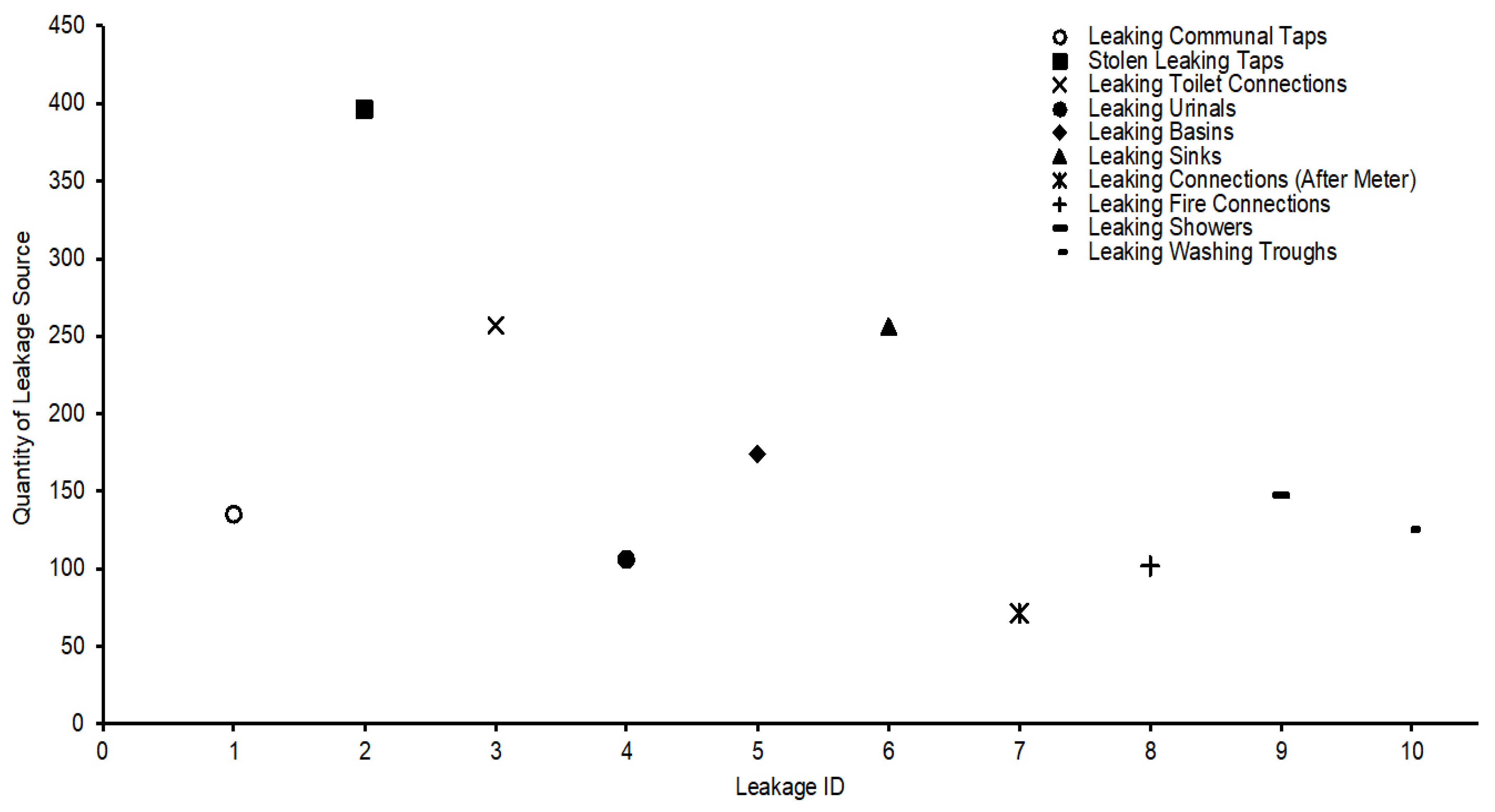
This section of the study presents the baseline data that were collected before the team could determine the total capital investment cost of retrofitting per household. Figure 2 shows the results obtained for the 110 randomly selected households inspected for domestic and background leakages (e.g., leaking taps and toilets). The results show that the 110 households produced combined leakage quantities of 1769 sources, with an average of 177 per household. From the socio-economic outlook of poverty and a lack of accountability from the residents, the results to some extent demonstrate that frequently leaking connections, toilets, sinks, and cisterns are among the highest contributors to domestic background leakage. Although the authors could not quantify the exact volumes that these leaking sources contributed to the overall NRW [8,25,36], the authors hold the view that items such as leaking service connections from households have a minimum leakage flow rate of 32 L/hour/m, as supported by Makaya [25]. This means that, with the number of leaking items presented in Figure 2, vast volumes of water are lost in the background daily. Therefore, it can be concluded that capital investment into the retrofitting, replacement, and repair of leaking and broken items such as taps and connections would greatly reduce MNF, NRW, and the overall SIV in Alexandra Township.
3.3.2. Customer Consumption Trends before and after SCIIS Implementation
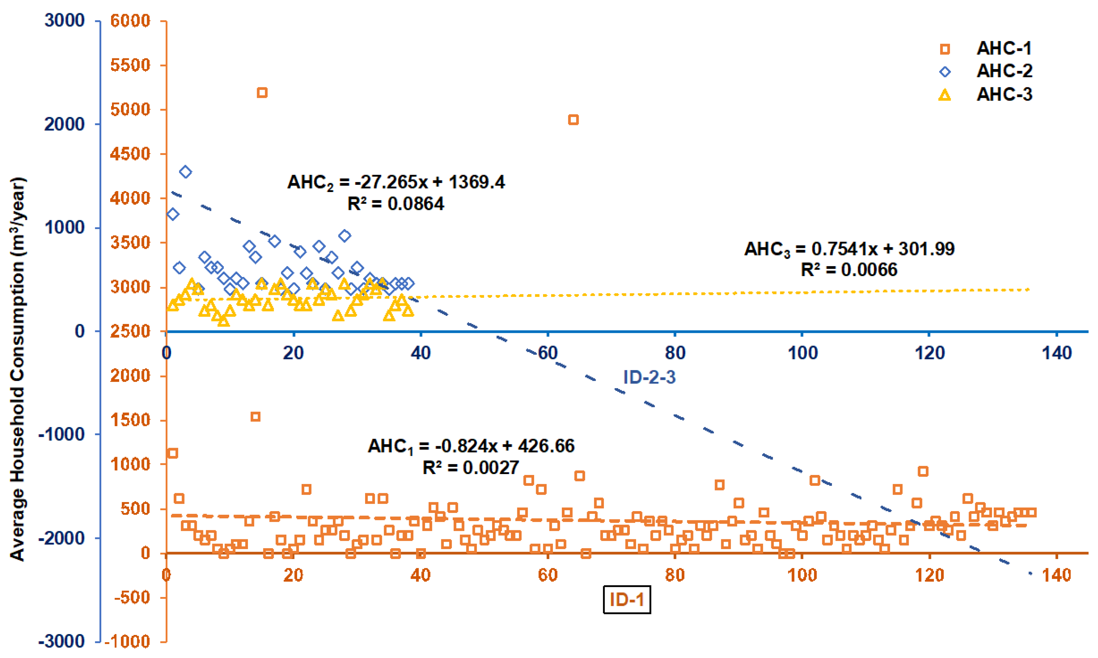
Figure 3 presents the average consumption pre- and post-retrofitting. The three-phase consumption results, denoted as AHC1, AHC2, and AHC3, were as follows:
Phase 1: The pre-results, denoted by the average household consumption (AHC1), represent the 136 randomly selected households, whose meters were manually read between 15 and 21 September 2020. The meter readings were aimed at establishing the average household consumption to assess whether the average household consumption (AHC) was higher than 360 m3/year, as recommended by Wegelin [36]. Higher recorded consumption normally indicates high background leakage, MNF, and NRW in the distribution system [11,36,37,38]. The results for AHC1 showed a linear reduction value (R2) of 0.0027, with a projected average consumption of 426.66 m3/year. According to Wegelin [36], such high consumption should be classified as commercial losses and unauthorized consumption. Although the projected AHC appears fair for denser residential areas such as Alexandra, some households recorded a projected AHC of 5000–5500 m3/year. The team then decided to randomly select a sub-set of 110 out of the 136 households to establish the sources of background leakage from households (Figure 2).
Phase 2: The corresponding results refer to the 38 households denoted by AHC2. These properties were selected as a sub-set of the 110 properties (Figure 2) that exhibited high consumption and excessive domestic background leakage. The results show that all 38 properties had an average linear consumption of 1369.4 m3/year at a linear reduction value (R2) of 0.0864, which is over three times that of the AHC derived during the AHC1 preliminary analysis. Therefore, the authors recommended to the water utility that all identified leakage sources (Figure 1) should be retrofitted under the “social capital investment intervention strategy (SCIIS)”. The capital funding for retrofitting was obtained from the Johannesburg Water SOC LTD regional maintenance office responsible for repair and maintenance of the water infrastructure in Alexandra Township.
Phase 3: The results for this phase are represented by AHC3. The 38 properties comprising the sub-dataset were retrofitted to reduce domestic background leakage. After the retrofitting capital investment project, customer meters were again read manually and consumption was recorded between 15 and 21 April 2021. The findings indicated a reduction in AHC from a constant value of 426 m3/year to 302 m3/year between AHC2 and AHC3. Furthermore, although the linear reduction values (R2) for AHC1, AHC2, and AHC3 appear insignificant, a decline in AHC during the three-phase approach is clearly evident (e.g., a decline from AHC2 = 1369.4 m3 to AHC3 = 301.99 m3/year). This projected annual consumption between AHC2 and AHC3 was 16.11% less than the 360 m3/year recommended threshold by Wegelin [36]), who outlined that consumption over 360 m3/year/household should be classified as commercial and unauthorized consumption. Therefore, the authors hold the opinion that implementation of the “social capital investment intervention strategy” (SCIIS) positively contributed to the overall reductions in NRW, MNF, and SIV in the water distribution system. The SCIIS unit cost per household was used to perform the sensitivity analysis during the cost–benefit analysis (CBA) indexes in the later sections of this study.
3.4. Total Water Leakage Method Results
3.4.1. Infrastructure Linear Leakage Repair
Table 4 shows the linear repair and maintenance outcomes abstracted from SAP-PM for a period of seven years, ranging from 1 July to the 31 June of the following year. These data were analyzed for the purpose of establishing leakage infrastructure trends and the associated costs of leakage reduction. The results show that between 2016 and 2020, the burst per kilometer ratio increased proportionally per annum. Furthermore, between 2015 and 2020, the average pressure increased year on year, which means more pressure was required to maintain the demand. The results show that linear leakage quantities averaged 3000 years on year between 2016 and 2020.
On the basis of the above assertion, the authors came to the preliminary conclusion that not only di AHC contribute to the high MNF and NRW, but infrastructure leakages also had an adverse effect on water loss problems in the study area. However, it is evident that during the 2021 calendar period, the average leakage quantity declined from an average of 3000 to 2671, whereas bursts per kilometer declined from 19 to 15 as compared to the previous year. This steady decline in the leakage indexes was achieved after the authors recommended the implementation of optimal pressure management in the water distribution system [12]. Finally, the established associated unit costs for repair and maintenance activities were used as a component of capital investment into leakage reduction and were integrated into the sensitivity analysis exercise of the CBA indexes. The corresponding findings are included in the later sections of this article.
3.4.2. Total Cost Method Results
Table 5 shows the total number of leakages and the corresponding total leakage flow rates (TLFR) over a 12-month period between 1 July 2020 and 31 July 2021. The mathematical formulation for average leak duration (ALD), the TLFR of the total annual volume of leakage (TAVL), and the total cost of water methods, as shown in Equations (3)–(5), were used to compute the results for reported bursts (RB), unreported bursts (URB), and leaking connections (LC). The results highlight that the overall volume of infrastructure leakage, measured as total leakage flow rates (TLFR) for all water losses in this study, equated to 13,840,704 m3/year at a converted value of USD 43.9 million. The TLFR represents 52.68%, against the computed NRW of 95.21% (Table 3).
This and other studies [9,10,12,13,24,36,39] indicate that improvements in the speed and quality of repairs by water utility repair and maintenance crews positively contribute to reducing the average leakage duration (ALD), the overall TLFR, and the associated operational costs. This is likely to lead in the long-term to a reduction in the MNF, NRW, and SIV in the distribution system. Similarly, the total costs of water leakages as components of reported bursts (RB), unreported bursts (URB), and leaking connections (LC) were used during the CBA index sensitivity analysis as outlined in the proceeding sections of this paper.
3.5. Cost–Benefit Analysis (CBA) Results
3.5.1. Overview
In the following sections we present the results of the CBA and the associated performance indexes. All data collected from the technical analysis and visual on-site assessment were integrated, costed using the total cost methods, and utilized during the CBA. The focus of this section is the evaluation of the three implemented water reduction strategies, namely, (i) pipe and infrastructure upgrade or renewal; (ii) operation and maintenance (O&M) costs; and (iii) the social capital investment intervention strategy (SCIIS).
3.5.2. Capital Investment on Water Loss Reduction and Marginal Cost of Capital
Table 6 shows the total cost method for the existing water loss reduction approaches currently being used in the case study area. The authors used the baseline data for SIV, MNF, and NRW for the years 2016/2017 and 2020 to determine the projected water loss trends and their cost for the period of 2021 to 2026 and beyond. All capital expenditure (CAPEX) as well as operations and maintenance cost investments into water losses were obtained from internal reports provided by Johannesburg Water (SOC) LTD, which is the water utility responsible for water provision in Alexandra Township.
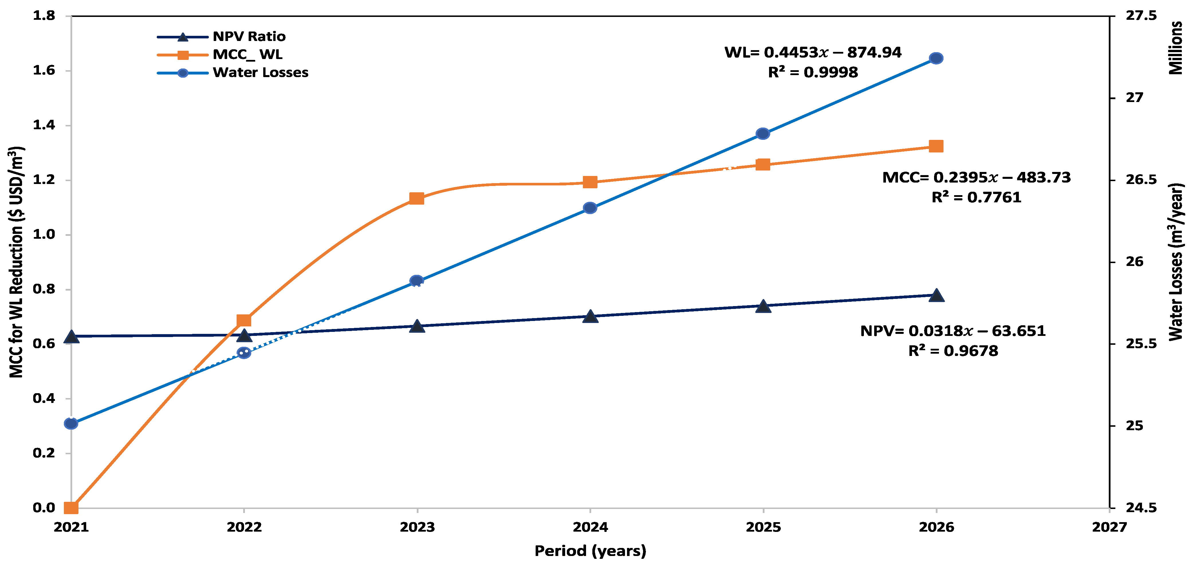
Table 6b shows the extended marginal cost of capital (MCC) for the two water loss (WL) reduction strategies in place, namely, (i) pipe and infrastructure upgrade or renewal and (ii) operation and maintenance (O&M). The comprehensive MCC and net present value (NPV) outlook results for Table 6 are graphically presented in Figure 4. The results show that between 2021 and mid-2025, the MCC remains higher than the average cost of water losses, which means that the water utility’s marginal investment is lower than the required net present value (NPV) ratio.
Other studies concluded that a lower MCC-versus-NPV ratio results in the non-achievement of the economic level of water leakage (ELWL) in capital water reduction [16,18,19,20,21,23]. The ELWL is the breakeven point, wherein the MCC graph intersects with the NPV and measures the allowable level of leakage per capital cost investment into a specific water loss reduction strategy [21]. The results show that linear reduction values (R2) of 0.7761 and 0.9998 for the MCC and water losses (WL), respectively, yield a constant ratio of 0.553 for MCC:WL, which means at least 55.3% of WL reduction capital investment is lost through leakage. Finally, the results may be interpreted as a prediction that, from the year 2026 and beyond, unless other WL reduction interventions are implemented, the cost of WL will continue to rise, whereas the MCC and NPV will remain low, thus making it impossible to achieve the ELWL.
3.5.3. Integrated Total Cost of Water Loss Trends
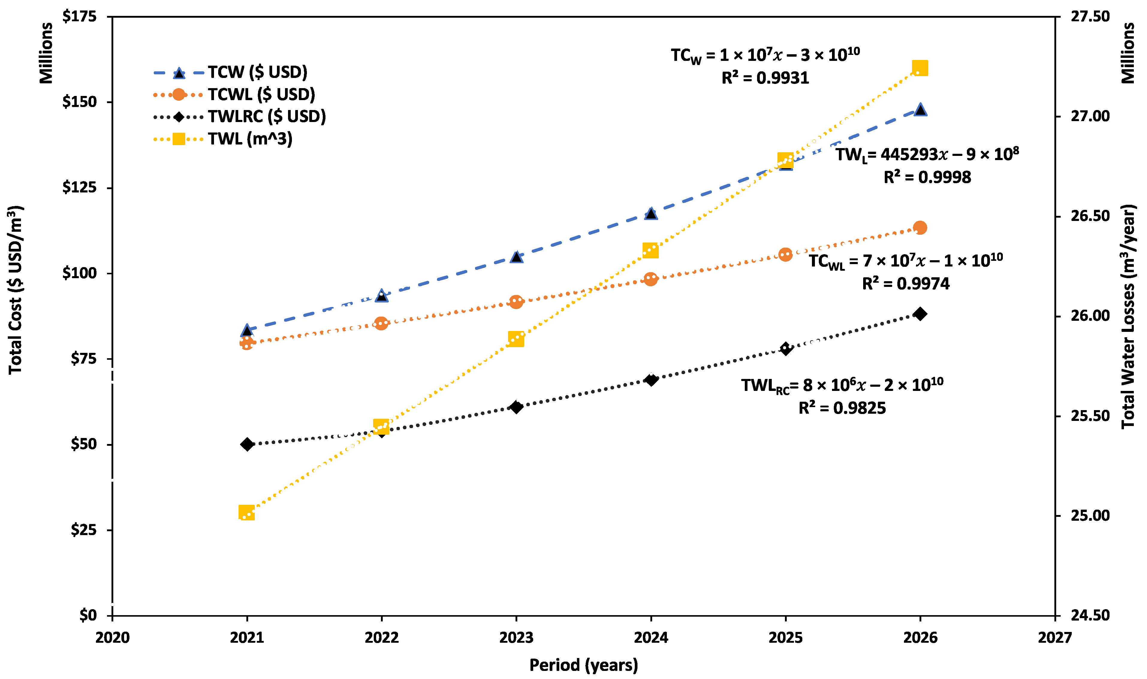
Figure 5 shows the integration of the total cost method in which non-revenue water (NRW) was compared with the total cost of water (TCW). The total cost of water losses (TCWL) were based on TLFR or TAVL (Equations (3)–(5) and Table 5). Furthermore, the total water loss reduction cost (TWLRC) was inclusive of the investment cost into CAPEX and O&M as water loss reduction strategies. The results for the year 2021 demonstrated that TCW and TWL increased with a similar trajectory, which was demonstrated by the almost equal linear values (R2) of 0.9931 and 0.9998, respectively. The projected results of TCW and TWL demonstrate that by 2026 almost 100% of the SIV will be regarded as NRW in the case study area, since the two water loss reduction strategies (CAPEX and O&M) are the only current options that the utility is presently investing in due to financial limitations. Financial limitations make it difficult for the water utility to curb water losses [35]. The financial limitations of water utilities are a common finding in some parts of the world [5,7,8,9,10,11,12,21,22,23,24,25,26]. The results indicate that in mid-2022 and 2025, the TWL graph intersected the TWLRC and TCWL graphs in an upward trajectory, which suggests that the cost of WL surpassed both the marginal production investment cost and the WL reduction capital investment. The results demonstrate that although WL reduction investments (CAPEX and O&M) are currently being implemented, they both yield minimum returns on investment (ROIs) for the water utility, since they are unlikely to achieve the ELWL. Therefore, the authors recommend that in order to achieve the ELWL, more WL reduction strategies should be developed by the water utility in Alexandra Township beyond CAPEX and O&M.
3.5.4. Sensitivity Analysis Investment Cost for the Total Leakage Flowrate
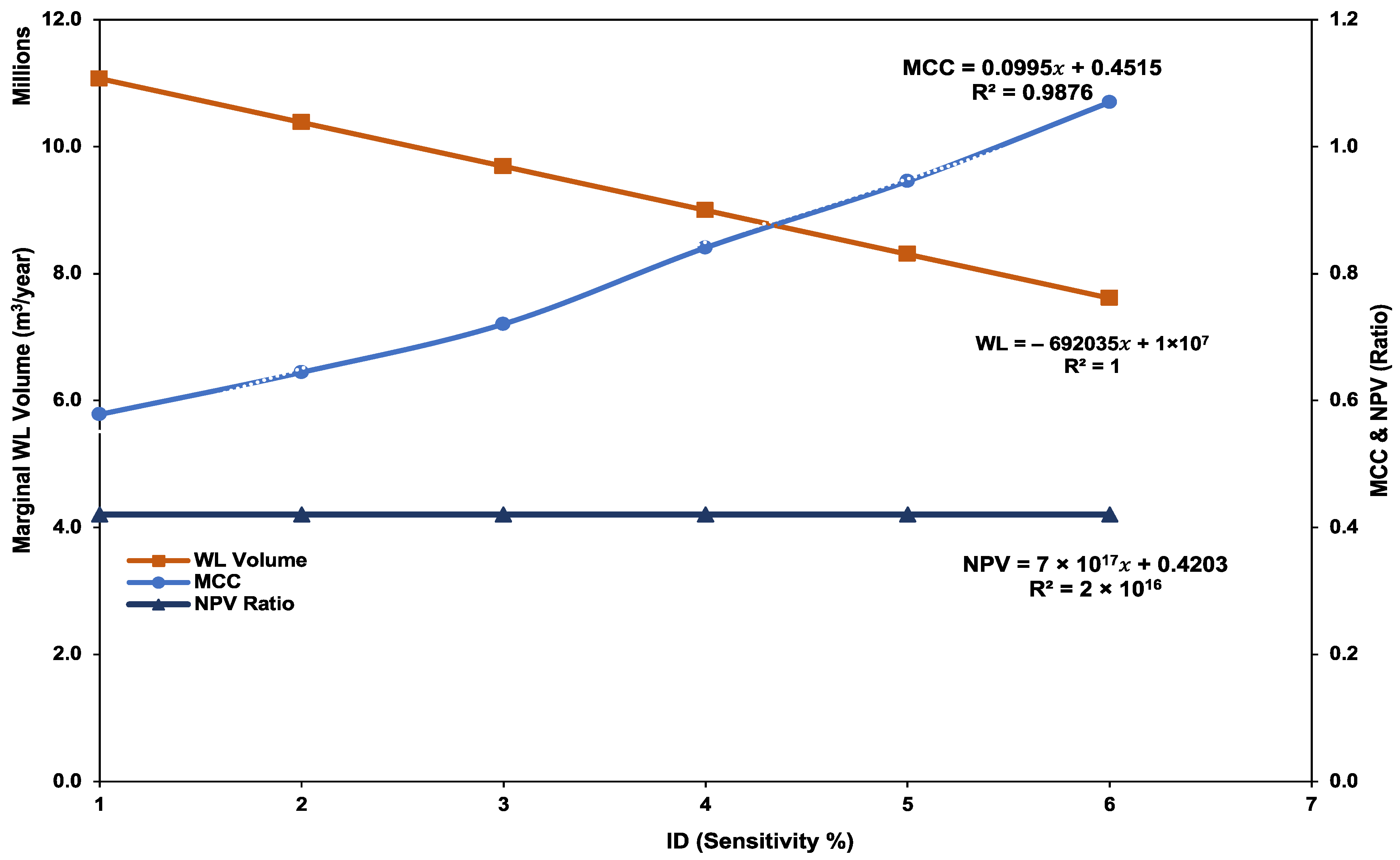
Figure 6 shows the sensitivity analysis results for TLFR reduction using the NPV ratio and MCC graphs and the attainment of ELL. This entailed deploying the trial-and-error method with the upward adjustment of the WL reduction investment until ELL was achieved. The results show that increments of WL reduction investment did not achieve the ELL. Moreover, the higher MCC versus NPV suggests that the low speed and quality of repairs cost the utility more when attending to leakages. Although the WL graph is constantly declining, the MCC increases, and thus, the ELWL remains unattainable. As the MCC investment ratio for TLFR reduction is not adequate, the authors recommend that a socio-technical approach may yield an adequate outcome.
3.5.5. Social Capital Investment Intervention Strategy and Marginal Cost of Capital
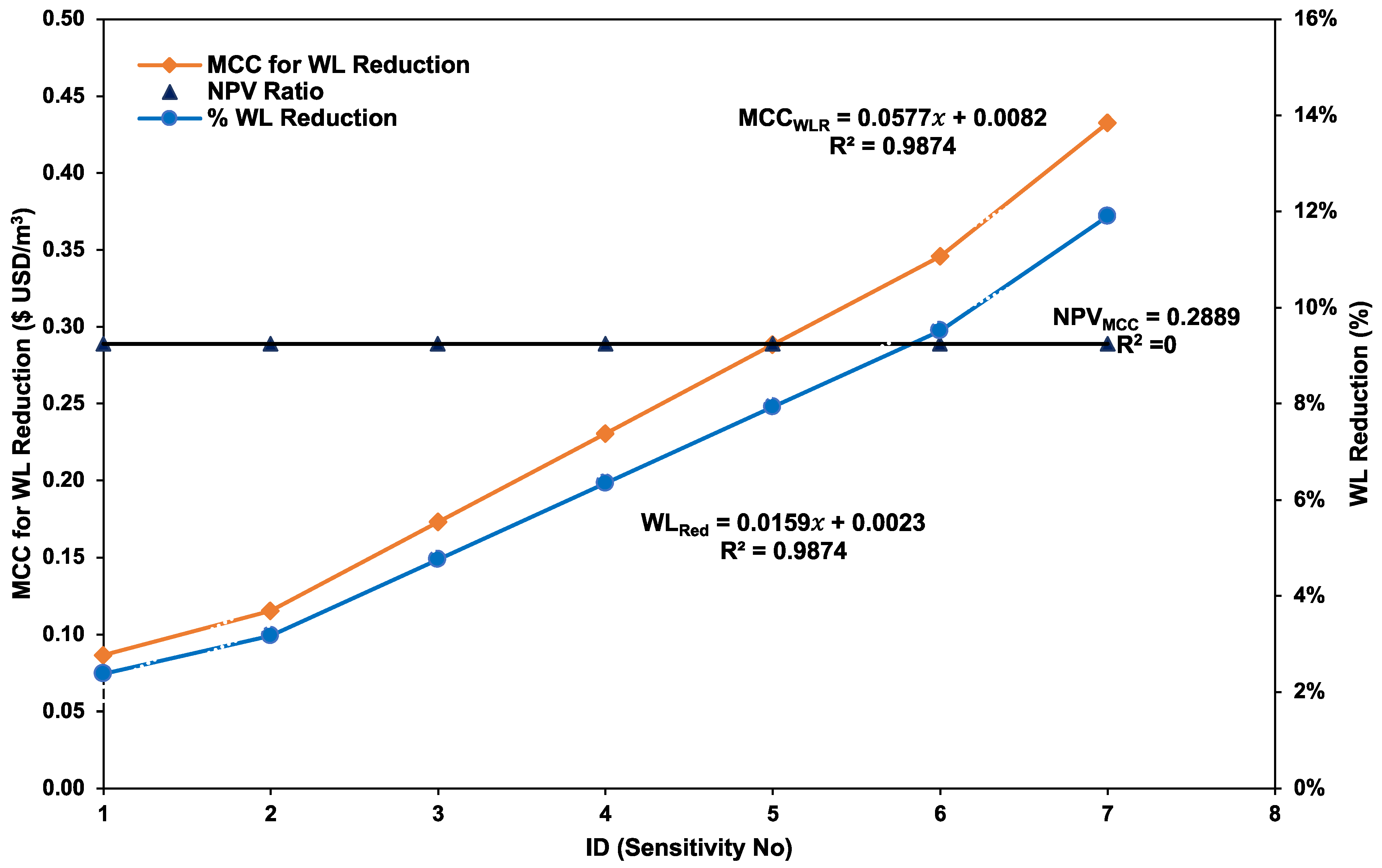
This section presents the CBA sensitivity analysis after applying the retrofitting process, which the authors call the social capital investment intervention strategy (SCIIS). Figure 7 shows the sensitivity analysis results for SCIIS for the 38 retrofitted properties. A cumulative total of 765 plumbing items were identified, retrofitted at an average cost of USD 5735/household and USD 217,917.30 in total. The results show that SCIIS implementation resulted in an average household saving of 521.05 m3/household/year. Moreover, to arrive at the ELWL on the MCC graph through the SCIIS strategy, the team performed a sensitivity analysis using a benchmark of 8000 properties with a steady percentage adjustment (using the trial-and-error method) of the dataset from 15% to 75%. The results show equal linear upward trends for MCC and WL at an R2 value of 0.9874, which means that implementing SCIIS yields a viable return on investment (ROI). The results also highlight that ELWL is achievable when MCC for retrofitting is increased proportionally to match WL reduction trends. Because implementing the CBA sensitivity analysis of SCIIS only measures customer consumption, the results demonstrate that WL reduction strategies that are social in nature are viable alternative ways of reducing domestic and background leakages. As demonstrated in the proceeding sections, wherein average household consumption (AHC) was reduced after retrofitting, it is clear that capital investment into the SCIIS program had positive results in terms of water loss reduction. The ELWL demonstrated by the MCC and NPV ratio indicates that the water utility should invest in this WL strategy, according to the authors.
3.5.6. Socio-Technical Sensitivity Analysis of Capital Net Risk
Table 7 shows the results for the socio-technical weighted average cost of capital (WACC), the coefficient of variance (CV), and the net risk analysis performed through the sensitivity analysis process. The authors combined all three water loss reduction strategies ((i) pipe and infrastructure upgrade or renewal, (ii) operation and maintenance (O&M) costs, and (iii) the social capital investment intervention strategy (SCIIS)) into a single WL capital investment. The team used the total cost method to combine the three water loss reduction capital investment strategies. The combination of the three WL strategies is what the authors refer to as the “socio-technical water loss control strategies”, and the overall capital structure was used to compute the WACC, CV, and capital net risk of the “socio-technical water loss control strategies”.
The results indicate that a combined WACC of 37.19% with the SCIIS contributes 0.001% of capital risk into water loss reduction. The low capital risk ratio for SCIIS is directly influenced by the 38 properties that were retrofitted, which is insignificant when compared with the other two strategies. Although the WACC for the SCIIS is insignificant, its return on investment (ROI) is noticeable in the MCC in the previous sections (Figure 7). When measuring the risk component of the SCISS using the CV, operation and maintenance costs show a lower risk of 0.08 as compared to SCIIS 0.41, which means SCIIS is almost 40% riskier to implement than the O&M.
The authors hold the opinion that the SCIIS risk is based on private investment. Other factors such as unaccountability, vandalism, and theft also contribute to the capital net risk of SCIIS. The results show that the socio-technical water loss control strategies’ risk-adjusted WACC of 0.66 and the net capital risk of 0.246 indicate that each WL reduction strategy shares a risk between 24.6% and 66%. Understanding of this shared risk assists water utilities in assessing where more resources should be invested to curb water losses. Accordingly, other studies [15,16,17,18,21] have attested to the value of the combined capital risk approaches and the distribution thereof, which water utilities must implement in their quest to curb water losses, specifically if more than one strategy is involved. Finally, the WCC and capital net risk required to demonstrate the ELWL for the socio-technical water loss control strategies, as displayed in Table 7, are summarized in Figure 8.
3.6. Socio-Technical Integrated Capital Net Risk Analysis Results
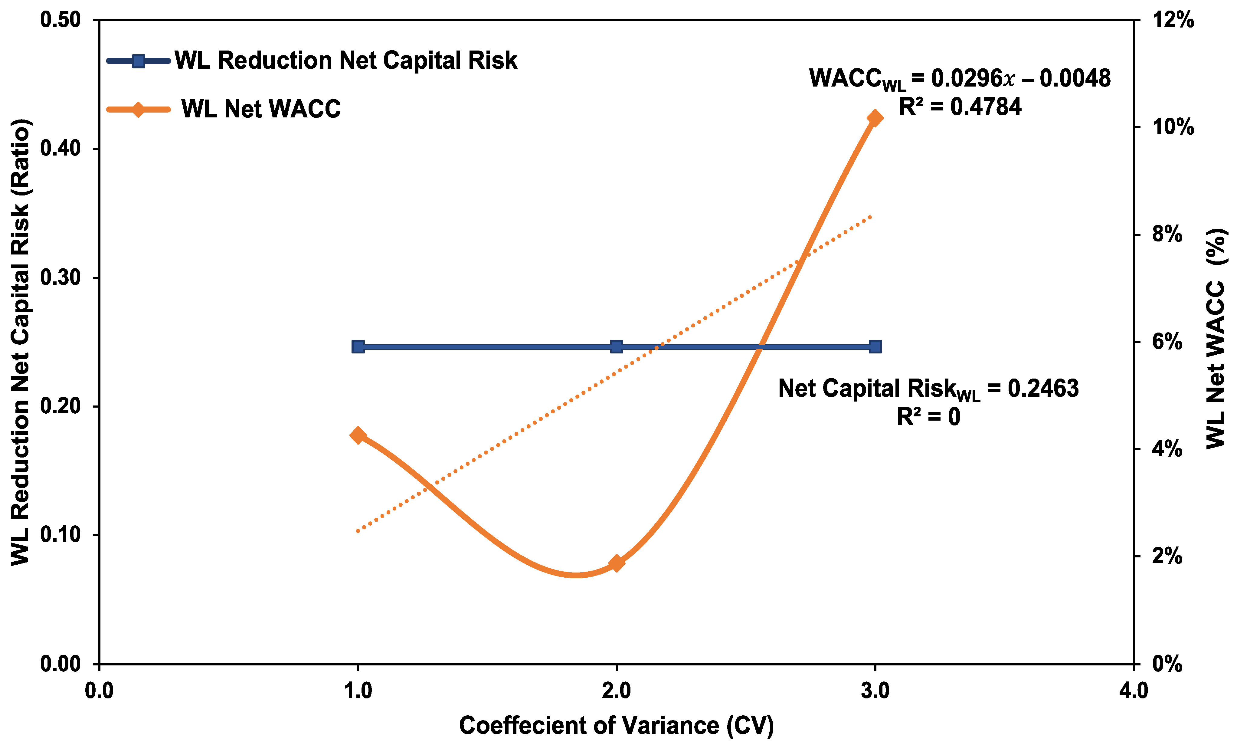
Figure 8 shows the WACC and the net capital risk for the socio-technical water loss control strategies derived from Table 7b. Figure 8 demonstrates where the ELWL was achieved, where the WACC intersects with the net capital risk graph. The net capital risk is an adjusted risk that is calculated by dividing the company’s total adjusted capital by the company’s risk weighed assets [19,20]. In this study, the weighted risk per water loss investment strategy was combined to make the overall WACC for the water loss capital investment, whereas the capital net risk per water loss strategy was regarded as a component of the NPV ratio. The idea of combining WACC per investment strategy and using capital net risk per strategy was inspired by the literature [19,20,30,31].
The results show that at an average risk variance of 2.5, the combined WACC for the socio-technical WL strategy produced the ELWL, which means that the water utility should invest 2.5 times more in annual water loss reduction capital to gradually continue towards the ELWL. As demonstrated in this study and supported by other studies [21,31], the ELWL can be identified as the point where the net capital risk or NPV intersects with the capital investments in the MCC graph. In other studies [19,20,21,31], the ELWL or breakeven point is where expenditure equals income and is a point where the capital risk of the project investment is zero.
Figure 8 also demonstrates that the socio-technical water loss control strategies’ linear reduction value (R2) of 0.4784 for WACC represents an upward trajectory, whereas the net capital risk R2 value is close to zero and on a constant horizontal plane. The authors’ preliminary inferences are that there are long-term marginal gains from the socio-technical water loss control strategies, and these could represent a highly effective method to reduce water losses in the long term. This opinion is supported by other studies that confirm that keeping net risk to a minimum in a company’s combined investment capital assets presents an opportunity to either break even on investment or achieve a return on it [19,20,21,29,30,31]. It follows that the combined and simultaneous implementation of the three water loss reduction strategies presents a viable alternative method to curb water losses in a complex socio-economic area such as the Alexandra Township.
4. Conclusions and Recommendations
The aim of this study was to present the benefits using CBA as part of a socio-technical water loss control strategy for a water supply network. The authors proposed three water loss reduction approaches: (i) capital investment in infrastructure upgrades, (ii) linear repair and maintenance capital investment, and (iii) the social capital investment intervention strategy (SCIIS) in a comparative approach. In this study, we utilized CBA performance indexes to achieve our objectives. Primary, the study results showed that after the implementation of SCIIS in Alexandra, the average household consumption (AHC) was reduced from about 1369 m3/year to 302 m3/year, which is a projected 77.84% average annual consumption saving. Furthermore, the findings indicated that existing water loss reduction strategies implemented by the water utility only yielded a water loss value of USD 44 million per year when measured as a component of the total leakage flow rate (TLFR), whereas the projected MCC was 55% of the NPV ratio. This finding shows that 45% of the existing capital investment on water reduction is lost through physical losses in the distribution system.
These two immediate outcomes projected a highly improbable and unattainable ELWL for the water utility. The total cost of water as a component of SIV versus total water losses as a component of NRW exhibited an upward trajectory, with R2 values of 0.99 and 1.00, respectively, and thus clearly indicated that by 2026, there is a likelihood that 100% of SIV will be recorded as NRW, which is exacerbated by various water leakage sources and a high MNF between 00:00 AM and 4:00 AM. The sensitivity analysis trajectory results showed that a reduction in TLFR to the ELWL is unlikely, because the MCC graph was moving away from the NPV ratio. The sensitivity analysis results for the SCIIS showed that 4000 properties at a unit cost of USD 5735 and water savings of 521 m3/year would achieve an ROI and ELWL on the MCC graph.
Finally, the individual results of the component analysis of (i) the linear reduction value R2 of 0.48, (ii) the integrated socio-technical risk-adjusted WACC of 16%, (iii) the CV of 0.66, and (iv) the combined NPV ratio or net capital risk of 0.25 and the reduction in the AHC clearly demonstrate that achieving the ELWL is possible when water loss reduction strategies, such as those presented in this paper, are implemented in an integrated manner (not in isolation). This is further proven by the fact that the individual findings of TLFR and AHC were higher before the implementation of SCIIS. The authors believe that most water utilities around the world should attempt to achieve ELWL by using a socio-technical approach in areas where high amounts of unaccounted water are lost due to domestic background leakages, as experienced by water managers in practice. Our findings should therefore persuade water managers and policy-makers, particularly in the developing world, to invest more resources towards socio-technical water loss reduction.
Author Contributions
Conceptualization, R.P.M. and M.S.; methodology, R.P.M.; software, R.P.M.; validation, R.P.M., M.S. and R.P.M.; formal analysis, R.P.M.; investigation, R.P.M.; resources, R.P.M.; data curation, R.P.M.; writing—original draft preparation, R.P.M.; writing—review and editing, M.S. and S.N.-B.; visualization, R.P.M.; supervision, M.S. and S.N.-B.; project administration, R.P.M.; funding acquisition, R.P.M. and M.S. All authors have read and agreed to the published version of the manuscript.
Funding
This research was financially supported by RainSolutions (Water JPI 2018 Joint Call project) via collaboration between Johannesburg University and Lund University.
Institutional Review Board Statement
The study was conducted according to the guidelines of the Declaration of the Department of Higher Education and Training of South Africa Government Gazette (No. 39583, Vol 607) of 8 January 2016 and originally approved by the University of Johannesburg on 12 February 2018 and the Institutional Review and Ethical committee of the University of Johannesburg on 24 August 2020 with the Ethical Clearance Number UJ_FEBE_FEPC_00034.
Informed Consent Statement
Informed consent was obtained from all subjects involved in the study and approved under Ethical Clearance Number UJ_FEBE_FEPC_00034.
Data Availability Statement
All generated and collected data, models, and code used during the study were provisionally and ethically granted by Johannesburg Water SOC Ltd. and the University of Johannesburg. Some or all of the data, models, and code that support the findings of this study are available from the corresponding author upon reasonable request.
Acknowledgments
The authors acknowledge the academic support from the University of Johannesburg and the data provided by Johannesburg Water SOC Ltd. (Johannesburg Metropolitan Municipality). This work was also supported by RainSolutions (Water JPI 2018 Joint Call project).
Conflicts of Interest
Risimati Patrick Mathye is an employee of Johannesburg Water SOC Ltd. However, the opinions expressed do not necessarily represent the views of Johannesburg Water SOC Ltd. The authors declare no conflict of interest. There are also no policy implications linked to the participating institutions.
References
- United Nations. Sustainable Development Goal 6: Synthesis Report on Water and Sanitation; UN-Water: New York, NY, USA, 2018. [Google Scholar]
- Boretti, A.; Rosa, L. Reassessing the projections of the World Water Development Report. NPJ Clean Water 2019, 2, 15. [Google Scholar] [CrossRef]
- Walker, A. The Independent Review of Charging for Household Water and Sewerage Services; Interim Report; Department for Environment, Food and Rural Affairs: London, UK, 2009.
- Mutikanga, H.E.; Sharma, S.; Vairavamoorthy, K. Water Loss Management in Developing Countries: Challenges and Prospects. J. Am. Water Works Assoc. 2009, 101, 57–68. [Google Scholar] [CrossRef]
- Dighade, R.R.; Kadu, M.S.; Pande, A.M. Challenges in Water Loss Management of Water Distribution Systems in Developing Countries. Int. J. Innov. Res. Sci. Eng. Technol. 2014, 3, 13838–13846. [Google Scholar]
- Colombo, A.F.; Karney, B.W. Energy and Costs of Leaky Pipes: Toward Comprehensive Picture. J. Water Resour. Plan. Manag. 2002, 128, 441–450. [Google Scholar] [CrossRef] [Green Version]
- Mathye, R.P.; Scholz, M.; Nyende-Byakika, S. Analysis of Domestic Consumption and Background Leakage Trends for Alexandra Township, South Africa. Int. J. Emerg. Technol. 2022, 13, 1–9. [Google Scholar]
- Makaya, E.; Hensel, O. The Contribution of leakage water to total water loss in Harare, Zimbabwe. Int. Res. J. 2014, 3, 55–63. [Google Scholar]
- Kanakoudis, V.K.; Gonelas, K. Applying pressure management to reduce water losses in two Greek cities’ WDSs: Expectations, problems, results and revisions. Procedia Eng. 2014, 1, 318–325. [Google Scholar] [CrossRef] [Green Version]
- Karadirek, I.E.; Kara, S.; Yilmaz, G.; Muhammetoglu, A.; Muhammetoglu, H. Implementation of Hydraulic Modelling for Water-loss Reduction through Pressure Management; Springer Science Business Media B.V: Berlin, Germany, 2011. [Google Scholar]
- McKenzie, R.S. Guidelines for Reducing Water Losses in South African Municipalities; Water Research Commission: Pretoria, South Africa, 2014. [Google Scholar]
- Mathye, R.P.; Scholz, M.; Nyende-Byakika, S. Optimal Pressure Management in Water Distribution Systems: Efficiency Indexes for Volumetric Cost Performance, Consumption and Linear Leakage Measurements. Water 2022, 14, 805. [Google Scholar] [CrossRef]
- Kanakoudis, V.; Gonelas, K. The Optimal Balance Point between NRW Reduction Measures, Full Water Costing and Water Pricing in Water Distribution Systems. Alternative Scenarios Forecasting the Kozani’s WDS Optimal Balance Point. Procedia Eng. 2015, 119, 1278–1287. [Google Scholar] [CrossRef] [Green Version]
- Venkatesh, G. CBA—Leakage reduction by rehabilitating old water pipelines: Case study of Oslo (Norway). Urban Water J. 2012, 9, 277–286. [Google Scholar] [CrossRef]
- Malm, A.; Moberg, F.; Roseén, L.; Pettersson, T.J.R. CBA and Uncertainty Analysis of Water Loss Reduction Measures: Case Study of the Gothenburg Drinking Water Distribution System. Water Resour. Manag. 2015, 29, 5451–5468. [Google Scholar] [CrossRef]
- Martins, R.; Coelho, F.; Fortunato, A. Water losses and hydrographical regions influence on the cost structure of the Portuguese water industry. J. Prod. Anal. 2012, 38, 81–94. [Google Scholar] [CrossRef] [Green Version]
- Molinos-Senante, M.; Mocholí-Arce, M.; Sala-Garrido, R. Estimating the environmental and resource costs of leakage in water distribution systems: A shadow price approach. Sci. Total Environ. 2016, 568, 180–188. [Google Scholar] [CrossRef] [PubMed]
- Ahopelto, S.; Vahala, R. Cost–Benefit Analysis of Leakage Reduction Methods in Water Supply Networks. Water 2020, 12, 195. [Google Scholar] [CrossRef] [Green Version]
- Lasher, W.R. Practical Financial Management, 8th ed.; Cengage Learning: Boston, MA, USA, 2014. [Google Scholar]
- Drury, C. Management Accounting for Business Management, 6th ed.; Cengage Learning EMEA: Boston, MA, USA, 2016. [Google Scholar]
- Heryanto, T.; Sharma, S.K.; Daniel, D.; Kennedy, M. Estimating the Economic Level of Water Losses (ELWL) in the Water Distribution System of the City of Malang, Indonesia. Sustainability 2021, 13, 6604. [Google Scholar] [CrossRef]
- Lim, E.; Savic, D.; Kapelan, Z. Development of a Leakage Target Setting Approach for South Korea Based on Economic Level of Leakage. Procedia Eng. 2015, 119, 120–129. [Google Scholar] [CrossRef] [Green Version]
- Lambert, A.; Fantozzi, M. Recent advances in calculating economic intervention frequency for active leakage control, and implications for calculation of economic leakage levels. Water Supply 2005, 5, 263–271. [Google Scholar] [CrossRef]
- Mutikanga, H.E.; Sharma, S.K.; Vairavamoorthy, K. Methods and Tools for Managing Losses in Water Distribution Systems. J. Water Resour. Plan. Manag. 2013, 139, 166–174. [Google Scholar] [CrossRef]
- Makaya, E. Water Loss Management Strategies for Developing Countries: Understanding the Dynamics of Water Leakages. Ph.D. Thesis, Universität Kassel/Witzenhausen, Harare, Zimbabwe, 2015. [Google Scholar]
- Mutikanga, H.E. Water Loss Management: Tools and Methods for Developing Countries. Ph.D. Thesis, Delft University of Technology, Leiden, The Netherlands, 2012. [Google Scholar]
- Ross, S.A. Uses, Abuses, and Alternatives to the Net-Present-Value Rule. Financ. Manag. 1995, 24, 96. [Google Scholar] [CrossRef]
- Mbabazise, P.M.; Daniel, T. Capital Budgeting Practices in Developing Countries: A case of Rwanda. Res. J. Financ. 2014, 2, 1–19. [Google Scholar]
- Banovec, P.; Domadenik, P. Defining Economic Level of Losses in Shadow: Identification of Parameters and Optimization Framework. Multidiscip. Digit. Publ. Inst. Proc. 2018, 2, 599. [Google Scholar] [CrossRef] [Green Version]
- Da, Z.; Guo, R.-J.; Jagannathan, R. CAPM for estimating the cost of equity capital: Interpreting the empirical evidence. J. Financ. Econ. 2012, 103, 204–220. [Google Scholar] [CrossRef]
- Schlegel, D. Background: Cost-of-capital in the finance literature. In Cost-of-Capital in Managerial Finance; Springer: Cham, Switzerland, 2015; pp. 9–70. [Google Scholar] [CrossRef]
- Albert, A.; Zhang, L. A novel definition of the multivariate coefficient of variation. Biom. J. 2010, 52, 667–675. [Google Scholar] [CrossRef] [PubMed]
- Wilson, M. Participatory Gender-Oriented Information and Learning Needs Assessment of the Youth of Alexandra; Background Report for UNESCO Developing Open Learning Communities for Gender Equity with the Support of ICTs; University of the Witwatersrand: Johannesburg, South Africa, 2002. [Google Scholar]
- Matowanyika, W. Impact of Alexandra Township on the Water Quality of the Jukskei River; A research report submitted to the Faculty of Science, University of the Witwatersrand; University of the Witwatersrand, Johannesburg, in partial fulfillment: Johannesburg, South Africa, 2010. [Google Scholar]
- WCWDM. Revised Water Conservation and Water Demand Management Strategy: Internal Report: Johannesburg Water: City of Johannesburg Metropolitan Municipality. WikiWater #227869. 2016. Available online: www.johannesburgwater.co.za (accessed on 20 April 2022).
- Wegelin, W.A. Guideline for a Robust Assessment of the Potential Savings from Water Conservation and Water Demand Management. Master’s Thesis, Faculty of Engineering at Stellenbosch University, Stellenbosch, South Africa, 2015. Available online: https://scholar.sun.ac.za (accessed on 20 April 2022).
- McKenzie, R. Development of a Standardised Approach to Evaluate Burst and Background Losses in Water Distribution Systems in South Africa; WRC, Report TT 109/99; Water Research Commission: Pretoria, South Africa, 1999. [Google Scholar]
- McKenzie, R.; Lambert, A.; South Africa Water Research Commission. ECONOLEAK: Economic Model for Leakage Management for Water Suppliers in South Africa, Users Guide; WRC Report TT 169/02; Water Research Commission: Pretoria, South Africa, 2002. [Google Scholar]
- Wu, Z.Y.; Farley, M.; Turtle, D.; Kapelan, Z.; Boxall, J.; Mounce, S.; Dahasahasra, S.; Mulay, M.; Kleiner, Y. Water Loss Reduction; Bentley Institute Press: Exton, PA, USA, 2011. [Google Scholar]
Figure 1.
Process flow diagram methodology.

Figure 2.
The socio-domestic and background leakage sources from households.

Figure 3.
Average customer consumption outcomes for the pre- and post-retrofitting process.

Figure 4.
The marginal cost of capital for existing water loss reduction: capital expenditure and operation and maintenance. MCC: marginal cost of capital, WL, water loss, NPV, net present value.
Figure 4.
The marginal cost of capital for existing water loss reduction: capital expenditure and operation and maintenance. MCC: marginal cost of capital, WL, water loss, NPV, net present value.

Figure 5.
Graphical results of the integrated total cost method. TCW: total cost of water, TCWL: total cost of water losses, TWLRC: total water loss reduction cost, TWL: total water loss.
Figure 5.
Graphical results of the integrated total cost method. TCW: total cost of water, TCWL: total cost of water losses, TWLRC: total water loss reduction cost, TWL: total water loss.

Figure 6.
Operation and maintenance sensitivity analysis graph for marginal cost of capital (MCC) and net present value (NPV). WL: water loss.
Figure 6.
Operation and maintenance sensitivity analysis graph for marginal cost of capital (MCC) and net present value (NPV). WL: water loss.

Figure 7.
Social capital investment intervention strategy for the social capital investment intervention strategy program. MCC: marginal cost of capital, NPV: net present value, WL: water loss.
Figure 7.
Social capital investment intervention strategy for the social capital investment intervention strategy program. MCC: marginal cost of capital, NPV: net present value, WL: water loss.

Figure 8.
Socio-technical approach of integrated weighted average cost of capital (WACC) and capital net risk outlook. WL: water loss.
Figure 8.
Socio-technical approach of integrated weighted average cost of capital (WACC) and capital net risk outlook. WL: water loss.


Table 1.
Mathematical formulations for the computation and derivation of the cost–benefit analysis indexes.
Table 1.
Mathematical formulations for the computation and derivation of the cost–benefit analysis indexes.
| Methodology | Mathematical Equation | References |
|---|---|---|
| Net Present Value (NPV) Ratio | is the period of compounding interest | [15,19,20,21,27,28,30,31] |
| Marginal Cost Capital (MCC) | [15,19,20,22] | |
| Weighted Average Cost of Capital (WCC) | is the compounding period in year, and CI is the value of NPV | [19,20,30,31,32] |
| Coefficient of Variance (CV) | where Xi is the individual value, N is the total dataset or number of values, is the mean average of the dataset, and P is the position of population dataset in a series | [19,20,32] |
Table 2.
Flow analysis results for the district metered areas.
| ID | Ave Flow (L/s) | Ave MNF (L/s) | Head (m) | SIV (m3/Year) | MNF (m3/Year) | % MNF/Ave Flow | % MNF/SIV |
|---|---|---|---|---|---|---|---|
| LP-1 | 70.1 | 56.40 | 180 | 2,209,412 | 296,438 | 81% | 13% |
| LP-2 | 343.8 | 296.10 | 80 | 10,843,338 | 1,556,302 | 86% | 14% |
| LP-3 | 248.5 | 202.10 | 90 | 7,836,696 | 1,062,238 | 81% | 14% |
| LP-4.1 | 9.3 | 8.18 | 50 | 293,285 | 42,984 | 88% | 15% |
| LP-4.2 | 2.7 | 1.34 | 51 | 85,147 | 6917 | 50% | 8% |
| LP-4.3 | 158.7 | 136.30 | 49 | 5,004,700 | 716,393 | 86% | 14% |
| 26,272,579 | 3,681,271 | Ave:79% | Ave:14% | ||||
SIV: system input volume, MNF: minimum night flow.
Table 3.
Water balance for Alexandra for the 2019/2020 financial year.
| System Input Volume (SIV) 26,272,578.53 m3/year. 100% | Authorized Consumption 17,676,052 m3/year. 67.28% | Billed Authorized Consumption 1,257,383.25 m3/year. 4.79% | Billed Metered Consumption 873,195.03 m3/year. 3.32% | Free Basic Water 337,902.5 m3/year. 1.29% |
| Billed Unmetered Consumption 384,188 m3/year. 1.46% | Recovered Revenue Water 919,480.71 m3/year. 3.5% | |||
| Unbilled Authorized Consumption 16,418,668.77 m3/year. 62.49% | Unbilled Metered Consumption No Historic Data 16,418,668.77 m3/year. 62.49% | Non-Revenue Water (NRW) 25,015,195.28 m3/year. 95.21% | ||
| Water Losses 8,596,526.51 m3/year. 32.72% | Apparent Losses No Historic Data 0 m3/year 0.00% | Real Looses + Unauthorized Consumption 8,596,526.51 m3/year. 32.72% | ||
| Real Losses 8,596,526.51 m3/year. 32.72% | Reservoir Overflows No Historic Data 0.00 m3/year 0.00% |
Table 4.
Linear repair and maintenance data (2015–2021).
| Description | Period | ||||||
|---|---|---|---|---|---|---|---|
| 2015 | 2016 | 2017 | 2018 | 2019 | 2020 | 2021 | |
| Reported Bursts (RB) | 1466 | 1517 | 1495 | 1403 | 1521 | 1567 | 1336 |
| Unreported Bursts (URB) | 299 | 216 | 233 | 254 | 209 | 264 | 179 |
| Burst Total (RB + URB) | 1765 | 1733 | 1728 | 1657 | 1730 | 1831 | 1515 |
| Leaking Connections (LC) | 1245 | 1145 | 1244 | 1324 | 1165 | 1211 | 1156 |
| Total (RB + URB + LC) | 3010 | 2878 | 2972 | 2981 | 2895 | 3042 | 2671 |
| Pipe Length (m) | 94,700 | 95,654 | 96,235 | 96,900 | 98,321 | 98,435 | 98,345 |
| Burst Frequency/km | 19 | 18 | 18 | 17 | 18 | 19 | 15 |
| Average Pressure (m) | 71.3 | 75.2 | 75.6 | 81.3 | 83.7 | 86.2 | 76.7 |
| Average Pipe Age (year) | 19.6 | 20.2 | 21.5 | 22.8 | 23.4 | 25.6 | 26 |
Table 5.
Total costs of infrastructure leakage quantities (2021).
| Reported Burst (RB) | Unreported Burst (URB) | Leaking Connection (LC) | Total Water Loss (TWL) USD/m3/Month | ||||||||||
|---|---|---|---|---|---|---|---|---|---|---|---|---|---|
| ID | RB No | ALD (h) | TAVL (m3) | UR No | ALD (h) | TAVL (m3) | LC No | ALD (h) | TAVL (m3) | TLFR (m3) | Total Cost (RB) | Total Cost (URB) | Total Cost (LC) |
| 1 | 123 | 31.20 | 921,024 | 15 | 73.55 | 132,390 | 103 | 61.01 | 201,089 | 1,254,503 | 2,928,856 | 421,000 | 639,463 |
| 2 | 131 | 31.20 | 980,928 | 22 | 73.55 | 194,172 | 112 | 61.01 | 218,660 | 1,393,760 | 3,119,351 | 617,467 | 695,338 |
| 3 | 134 | 31.20 | 1,003,392 | 10 | 73.55 | 88,260 | 111 | 61.01 | 216,708 | 1,308,360 | 3,190,787 | 280,667 | 689,130 |
| 4 | 120 | 31.20 | 898,560 | 13 | 73.55 | 114,738 | 119 | 61.01 | 232,326 | 1,245,624 | 2,857,421 | 364,867 | 738,797 |
| 5 | 126 | 31.20 | 943,488 | 12 | 73.55 | 105,912 | 98 | 61.01 | 191,327 | 1,240,727 | 3,000,292 | 336,800 | 608,421 |
| 6 | 119 | 31.20 | 891,072 | 15 | 73.55 | 132,390 | 112 | 61.01 | 218,660 | 1,242,122 | 2,833,609 | 421,000 | 695,338 |
| 7 | 125 | 31.20 | 936,000 | 13 | 73.55 | 114,738 | 89 | 61.01 | 173,756 | 1,224,494 | 2,976,480 | 364,867 | 552,546 |
| 8 | 132 | 31.20 | 988,416 | 22 | 73.55 | 194,172 | 110 | 61.01 | 214,755 | 1,397,343 | 3,143,163 | 617,467 | 682,922 |
| 9 | 102 | 31.20 | 763,776 | 19 | 73.55 | 167,694 | 78 | 61.01 | 152,281 | 1,083,751 | 2,428,808 | 533,267 | 484,253 |
| 10 | 86 | 31.20 | 643,968 | 10 | 73.55 | 88,260 | 83 | 61.01 | 162,043 | 894,271 | 2,047,818 | 280,667 | 515,295 |
| 11 | 67 | 31.20 | 501,696 | 16 | 73.55 | 141,216 | 76 | 61.01 | 148,376 | 791,288 | 1,595,393 | 449,067 | 471,837 |
| 12 | 71 | 31.20 | 531,648 | 12 | 73.55 | 105,912 | 65 | 61.01 | 126,901 | 764,461 | 1,690,641 | 336,800 | 403,545 |
| Total Cost/year | 31,812,618 | 5,023,936 | 7,176,885 | ||||||||||
ALD: average leak duration, TAVL: total annual volume of leakages.
Table 6.
(a) Preliminary technical water loss reduction investment data; and (b) the marginal cost of capital for water loss reduction investment.
Table 6.
(a) Preliminary technical water loss reduction investment data; and (b) the marginal cost of capital for water loss reduction investment.
| (a) | ||||||||
| Total Cost Method (USD) | Total WL Reduction Cost (USD) | |||||||
| Period | Total WLNRW | Unit Cost/m3 | Cost of WL | SIV | Total Cost of Water | CAPEX | O&M | WL Reduction Cost |
| 2016/17 | 15.69 | 2.31 | 36.23 | 18.03 | 41.64 | 18.72 | 0 | 18.72 |
| 2017/18 | - | 2.46 | - | - | - | 20.83 | 0 | 20.83 |
| 2018/19 | - | 2.62 | - | - | - | 25.27 | 0 | 25.27 |
| 2019/20 | - | 2.79 | - | - | - | 27.78 | 0 | 27.78 |
| 2020/21 | - | 2.97 | - | - | - | 33.67 | 16.37 | 50.04 |
| 2021/22 | 25.02 | 3.18 | 79.55 | 26.27 | 83.55 | 35.53 | 18.50 | 54.03 |
| SUM:(5 yrs.) | 40.70 | 16.33 | 115.78 | 44.30 | 125.19 | 161.80 | 34.87 | 196.67 |
| Diff/yr. | 9.33 | - | 43.31 | 8.25 | 41.91 | - | 18.50 | 54,032 |
| Av. Diff/yr. | 1.89 | 3.27 | 8.66 | 1.65 | 8.38 | 32.36 | - | - |
| % Diff/yr. | 37.29 | 27.36 | 54.45 | 31.39 | 50.16 | 47.31 | 100 | 65.35 |
| % Av./5 yr. | 7 | 5.5 | 10.89 | 6. 28 | 10.89 | 9.46 | - | 13.07 |
| 2016/17: WLNRW @ 87.02%; 2020 WLNRW @ 95.21%; Cost (USD and Volume (m3) in millions) | ||||||||
| (b) | ||||||||
| Description and Period | 2021 | 2022 | 2023 | 2024 | 2025 | 2026 | ||
| WL Control Investment Cost (Million USD) | 50.04 | 54.03 | 61.10 | 69.08 | 78.11 | 88.32 | ||
| Incremental WL Cost (Million USD) | - | 3.99 | 7.06 | 7.99 | 9.03 | 10.21 | ||
| WL Component of Non-revenue Water (Million USD/m3) | 79.55 | 85.37 | 91.61 | 98.31 | 105.50 | 113.22 | ||
| WL Reduction Cumulative Difference | 5.82 | 6.24 | 6.70 | 7.19 | 7.72 | |||
| Marginal Cost of WL (Million USD/m3) | 0.686 | 1.131 | 1.192 | 1.256 | 1.323 | |||
| Water Loss (m3/year) | 25.02 | 25.45 | 25.88 | 26.33 | 26.78 | 27.24 | ||
| Net Present Value Ratio | 0.63 | 0.63 | 0.67 | 0.70 | 0.74 | |||
WL: water level, SIV: system input volume, CAPEX: capital expenditure. O&M: operation and maintenance.
Table 7.
(a) Weighted cost of capital for combined socio-technical water loss reduction; and (b) sensitivity analysis for weighted average cost of capital (WACC) concerning socio-technical water loss (WL) reduction.
Table 7.
(a) Weighted cost of capital for combined socio-technical water loss reduction; and (b) sensitivity analysis for weighted average cost of capital (WACC) concerning socio-technical water loss (WL) reduction.
| (a) | ||||||||||
|---|---|---|---|---|---|---|---|---|---|---|
| Total WL Investment Cost (USD) (A) | Capital Investment Weight (%) (B1; B2; B3) | Total WL Cost (USD) (C) | Weight of Capital/Total WL Cost (%) (D1; D2; D3) | WACC Value (%) (E1; E2; E3) | ||||||
| Description | ||||||||||
| WL Capital Expenditure (X) | 35,534,591 | 65.50 | 79,548,320 | 44.67 | 29.260 | |||||
| Operations and Maintenance (Y) | 18,498,113 | 34.10 | 79,548,320 | 23.25 | 7.929 | |||||
| Social Capital Investment (Z) | 217,917.30 | 0.40 | 79,548,320 | 0.27 | 0.001 | |||||
| SUM (USD) | 54,250,621.70 | 100.00 | - | 68.20% | ||||||
| Sum of Combined WACC = 37.19 | ||||||||||
| Formulae: B1 = (X/SUM); B2 = (Y/SUM); B3 = (Z/SUM); D = (A/C) × 100; E = (B/100) × (100 × D): SUM: (B1 + B2 + B3) | ||||||||||
| (b) | ||||||||||
| Period | WL Sensitivity Analysis Index | |||||||||
| Description | 2022 | 2023 | 2024 | 2025 | 2026 | Mean | Standard Deviation | CV | Net WACC | Capital Risk |
| Capital Expenditure Index (USD mill) | 54,032 | 61,094 | 69,079 | 78,108 | 88,317 | 70,126 | 12,135 | 0.17 | 4.2% | 0.246 |
| Operation and Maintenance Sensitivity Index (USD mill) | 20,347 | 21,272 | 22,197 | 24,047 | 24,972 | 22,567 | 1715 | 0.08 | 2% | 0.246 |
| Social Capital Investment Intervention Strategy Sensitivity Index (USD mill) | 6881 | 9175 | 13,763 | 18,350 | 22,938 | 14,221 | 5875 | 0.41 | 10% | 0.246 |
| Average Net WACC Risk = WACC Value × Sum CV e.g., (37.19% × 0.66 = 0.246) Net WACC = (Average Net WACC Risk × CV); e.g., (0.246 × 0.17) × 100 = 4.2% | Combined CV/Risk: 0.66 Net Capital Risk: 0.246 | |||||||||
Publisher’s Note: MDPI stays neutral with regard to jurisdictional claims in published maps and institutional affiliations. |
© 2022 by the authors. Licensee MDPI, Basel, Switzerland. This article is an open access article distributed under the terms and conditions of the Creative Commons Attribution (CC BY) license (https://creativecommons.org/licenses/by/4.0/).
Share and Cite
MDPI and ACS Style
Mathye, R.P.; Scholz, M.; Nyende-Byakika, S. Appraisal of Socio-Technical Water Loss Control Strategies Using Cost-Benefit Analysis in a Water Supply Network. Water 2022, 14, 1789. https://doi.org/10.3390/w14111789
AMA Style
Mathye RP, Scholz M, Nyende-Byakika S. Appraisal of Socio-Technical Water Loss Control Strategies Using Cost-Benefit Analysis in a Water Supply Network. Water. 2022; 14(11):1789. https://doi.org/10.3390/w14111789
Chicago/Turabian StyleMathye, Risimati Patrick, Miklas Scholz, and Stephen Nyende-Byakika. 2022. "Appraisal of Socio-Technical Water Loss Control Strategies Using Cost-Benefit Analysis in a Water Supply Network" Water 14, no. 11: 1789. https://doi.org/10.3390/w14111789
Note that from the first issue of 2016, this journal uses article numbers instead of page numbers. See further details here.