Numerical Simulation of Internal Flow Characteristics and Pressure Fluctuation in Deceleration Process of Bulb Tubular Pump

Abstract

In order to explore the change in internal and external characteristics and the pressure fluctuation of the large bulb tubular pump unit during deceleration, a transient and steady three-dimensional (3D) numerical simulation is executed, based on the standard k-ε turbulence model and the change in boundary conditions such as flow rate. Finally, the pressure fluctuation data are analyzed by the wavelet method. There is a good agreement between the experimental data and numerical simulation results. During the deceleration process of the unit, the head decreases linearly while the efficiency remains stable. Meanwhile, the shock phenomenon and hysteresis effect appear before and after the unit head deceleration. Although there are vortex and backflow in the outlet conduit during deceleration, the pressure distribution on the suction surface of the impeller blades changes uniformly and significantly. The pressure fluctuation changes on the inlet surface of the impeller are more obvious during the deceleration: the closer to the hub, the greater the pressure, and this change decreases with decreasing radius. The fluctuation energy is mainly concentrated in the high-frequency region of 100–120 Hz and decreases uniformly with the deceleration of the rotational speed. This paper provides a reference for the energy utilization and safe operation of the water pump unit in adjusting speeds with variable frequency.

1. Introduction

A pump that can convert mechanical energy into liquid kinetic energy and convey fluid directionally has been widely used in many fields [1]. Among the different types of pumps, the tubular pump is widely used in low-head pumping stations due to its several advantages, such as high efficiency, good hydraulic performance, and compact structure [2]. Compared with the axial-flow pump and the mixed-flow pump, the use of the tubular pump unit can reduce the amount of excavation of the factory and the concrete needed, and then greatly reduce the overall cost of the pumping station [3,4].

Although the hydraulic performance of the tubular pump is stable under the designed operating condition, the operation point of the pump will inevitably alter due to the change in the internal and external factors. In order to ensure the efficient and reliable operation of the pump to reduce energy consumption and mechanical losses, adjusting the speed with Variable-Frequency Drives (VFDs) is one of the effective and feasible methods. As part of the Eastern Route of South-to-North Water Diversion Project, many large-scale tubular pumping stations have made use of adjusting the speed with VFDs to regulate the operation point to achieve the best efficiency point [5].

The one-dimensional (1D) flow model is an effective method that balances computational accuracy and speed, which is used to analyze flow characteristics and pressure distribution normally. Gu et al. [6,7] established a new self-closed 1D pressure model by introducing Poncet’s K formula. Based on the above theory, the pressure of the casing wall can be predicted well. They also proved that the rotating speed is related to thrust acting on the shrouds, which has little effect on volumetric efficiency. Taking into consideration the blade slip factor, the self-closed 1D pressure model was later improved and the calculated results presented a greater agreement with the experimental data. Song et al. [8] investigated the free surface vortex by establishing a theoretical model of the pressure fluctuation induced by the linear vortex according to the Biot–Savart Law. There was a great agreement between the results of theoretical analysis and model experiments.

Although the method of 1D models can be used to increase the calculation speed as a good compromise of solution accuracy and computation feasibility, experimentation and computational fluid dynamics (CFD) are the most important ways for researchers to investigate hydraulic problems. With the development and wide use of CFD, scholars normally validate the two against each other to increase the credibility of the study and capture the complex flow features in hydraulic machines [9]. Shi et al. [10] designed an axial-flow pump runner by using the method of the surface element based on plane cascade theory. The hydraulic performances of the impeller, calculated by the CFD and model test, showed great agreement with each other. Shi et al. [11] optimized the comprehensive performance of the axial-flow pump with the objective of light weight and high efficiency. The reliability was verified by CFD and model tests, which proved that the accuracy of the approximate model used was high. Yang et al. [12] studied the impact on the hydraulic performance caused by different tip clearance sizes of a sewage pump. Meanwhile, the investigation of the complex vortices structure and propagation benefited from the 3D numerical simulation and test verification. The pressure fluctuation is an important characteristic that reflects the operating state of the water pump. The method of CFD is used to study the pressure fluctuation, which is an important way for the study of the stable operation of the pump. Liu et al. [13] investigated the flow and external characteristics of the pump mode turbine in the hump region, based on the SST turbulence model, and proved that the rotating speed determines the characteristics of pressure fluctuation at the wave trough of the hump region. Andreas et al. [14] implemented comparative research on the highly transient flow field in single and double-vane pumps. Based on the mutual verification of experiments and numerical simulations, the characteristics of flow rate and pressure fluctuation on single and double-vane pumps were summarized. Song et al. [15,16] studied the formation mechanism and the dynamic characteristics of the free surface vortex in the pump sump and the effect on the performance of the pump by numerical simulation.

In recent years, many domestic and foreign scholars have carried out a large number of studies on the variable-speed transient process of fluid machinery, but they mainly focused on the unit start-up and shutdown process. Tsukamoto et al. [17] developed theories to predict the transient characteristics of the centrifugal pump during deceleration and proved that the difference between dynamic and quasi-steady characteristics mainly come from impulsive pressure and lag around the vanes. Liu et al. [18] numerically simulated the rapid stopping process of the pump. They found that at the beginning of deceleration, the pressure fluctuation of the pump decreased but the pressure at the inlet increased. Meanwhile, the deviation in the quasi-steady and transient calculation results was attributed to the difference in the internal vortex of the impeller. Chalghoum et al. [19] investigated the dynamic characteristics of the centrifugal pump start-up process under different valve openings and the influence of impeller parameters on pressure changes. Zhang et al. [20,21] numerically investigated the system performance and affinity issue of the tubular pump under variable rotating speed operations. He proved that the similarity law cannot predict the relationship between head and discharge rates during the speed change process completely accurately, but within a certain speed range, the predicted error is acceptable.

However, some characteristics of the large-scale bulb tubular pump unit under the variable-speed operation, such as the pressure fluctuation and distribution, have not been analyzed. There is still room for studies. Therefore, this paper aims to investigate those characteristics of the tubular pump unit, under the operation of rotating speed deceleration (from 1223 rpm to 978.5 rpm), by the methods of CFD and model test. Section 2 describes the computational model and numerical method. Section 3 compares the data of the model test and CFD. The accuracy and reliability of numerical results are verified. The variable speed characteristics calculated by numerical simulation are presented and analyzed in Section 4, and Section 5 summarizes some important conclusions.

2. CFD Method

2.1. Computation Module

The prototype pump in the South-to-North Water Diversion Project with the S-shaped blades is 3350ZGQ37.5-2.45 and the corresponding rated power is 2200 kW. Taking into consideration the exited model test data, this paper established the horizontal bulb tubular pump model components, including inlet conduit, impeller, guide vanes, and outlet conduit, by UG12.0. The main parameters of the bulb tubular pump model are listed in

Table 1. Characteristic parameters of pump model flow system.

Parameters	Value
Diameter of impeller/mm	315
Number of impeller blades/-	3
Number of guide vanes/-	5
Number of front support vanes/-	6
Blade angle/°	0
Design head/m	2.45
Design discharge/m3/min	19.9
Initial rotating speed/r/min	1223
Target rotating speed/r/min	978.5 (20% deceleration)

. The computational fluid region was the entire unit from the inlet section of the inlet conduit to the outlet of the outlet conduit, and the 3D model of the horizontal bulb tubular pump is shown in Figure 1.

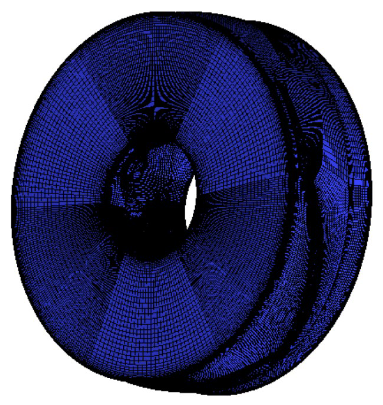
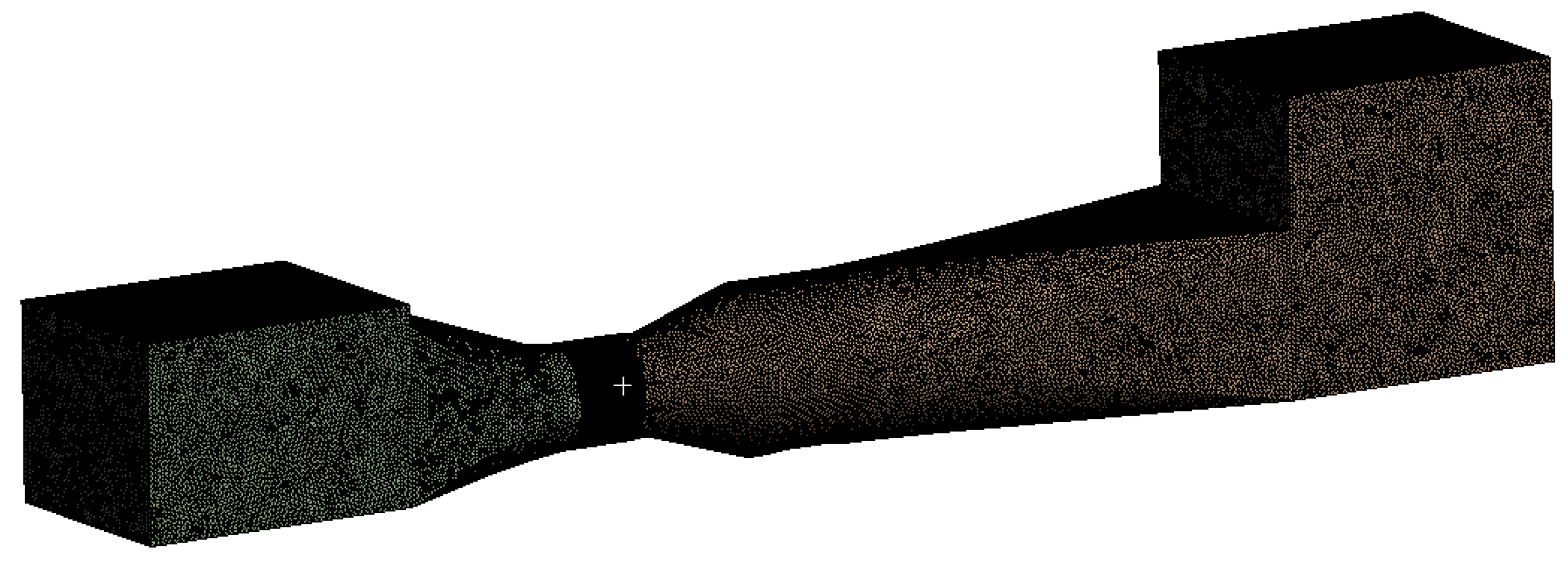
2.2. Hexahedral and Tetrahedral Mesh

Each part of the computational fluid domain was spat first and then assembled in ANSYS CFX after meshing. In order to take into consideration the later calculation efficiency and accuracy, the hexahedral mesh shown in Figure 2 was generated by using ANSYS ICEM CFD for the impeller portion of the computational model. By controlling the nodes on each topology line, the grid encryption degree of the impeller part is ensured, which is shown in the darker part of Figure 3. The other tetrahedral mesh of the calculation domain was generated by ANSYS MESH. In this paper, the grid independence test was carried out on the grid number of the inlet conduit of the large-scale bulb tubular pumping station during the stable operation under the design conditions. The mesh of the inlet conduit was generated with the same method to ensure that the number of grids changed without reducing quality. Through the steady calculation, it was found that when the number of grids in the calculation domain reached about 4.3 million (Figure 3), the change in hydraulic loss was controlled within ±5%, which met the requirement of the grid independence test. As shown in Figure 4, the total number of grid cells in the fluid region was 12,261,547, of which the number of grid cells in the impeller part was 1,760,000.

2.3. Computational Setup

Both a steady and transient 3D simulation of this large-scale bulk tubular pump was conducted by ANSYS CFX based on Reynolds-averaged Navier-Stokes equations (RANS). The results of the steady simulation were calculated first and taken as the initial value of the unsteady simulation. It is important to select an appropriate turbulence model to simulate the complex flow field inside the pump unit. Taking into consideration the compromise of solution accuracy and computation feasibility, the standard k-ε model can capture the internal transient flow characteristics of the pump under speed change operation well [22]. Therefore, this one was selected as the turbulence model to close the governing equations, and the SIMPLEC algorithm was used to solve the discrete algebraic equations.

The “Frozen Rotor” interface was used to connect the rotating domain and the stationary domain in the steady numerical simulation, and the “Transient Frozen Rotor” mode was used to transmit data through the interface based on interpolation in the transient numerical simulation. All solid walls were specified with smooth and nonslip, and the calculation medium was normal-temperature water. The boundary condition at the pump outlet was set as total pressure, and the mass flow rate was specified at the pump inlet.

What the paper focused on was the variable-speed characteristics, and it should be carefully considered when the rotating speed of impeller was set. It can be assumed that the efficiency of the pump unit does not change when the pump operates in a certain rotating speed range [19]. Based on the above assumption of constant efficiency, the pump performance parameters at variable speeds are shown as follows:

$$\{\begin{array}{l}\frac{Q_1}{Q_2}=\frac{n_1}{n_2}\\ \frac{H_1}{H_2}={\left(\frac{n_1}{n_2}\right)}^2\\ \frac{P_1}{P_2}={\left(\frac{n_1}{n_2}\right)}^3\end{array}$$

(1)

where Q_i, P_i, H_i, and n_i are the flow rate, shaft power, efficiency, and speed of the pump under the working condition of i, respectively. It is obvious that the flow rate at the pump inlet will reduce in accompaniment with the rotating speed deceleration. According to the above equations, under the assumption of constant efficiency, the discharge rate of the unit could be achieved by

$$Q=Q_d\times \frac{n}{n_d}$$

(2)

where Q_d and n_d are the discharge rate and rotating speed of pump under the design condition, respectively, n is the pump rotating speed under running, and Q is the discharge rate corresponding to n.

Based on the above theories, the algorithm of variable speed was implemented at the rotating domain, through the CFD secondary development (CFX Expression Language): the impeller rotating speed change was set as uniform deceleration from 1223 rpm to 978.5 rpm and the costed time was 1.5 s. The relationship between the rotating speed and the mass flow rate set at the inlet is shown in Figure 5. According to the curve characteristics of Figure 6 in Reference [23], in the first half of the deceleration, the rotating speed and flow rate showed the same trend, conforming to Equation (1), so the setting of the inlet boundary conditions was feasible. In the transient simulation, the total time was set to 3.5424 s, and each time step was set to 0.00246 s, which corresponds to an impeller rotation of 18 deg. The maximum iteration number in each time step was set to 20, and the residual convergence accuracy was set to 10⁻⁴.

2.4. Methods of Pressure Fluctuation Analysis

As the pressure fluctuation during the speed change is an unsteady signal, the Fast Fourier Transform (FFT) with a fixed-size analysis window cannot fully reflect the time and frequency characteristics. Therefore, the wavelet method was used to analyze the unsteady pressure fluctuation signal in the process of speed change of the model pump in this paper. Compared with the method of FFT, wavelet analysis has a good ability to characterize signals in both time and frequency domains, and has a better adaptability to signals [24].

3. Comparison of CFD with Experimental Results

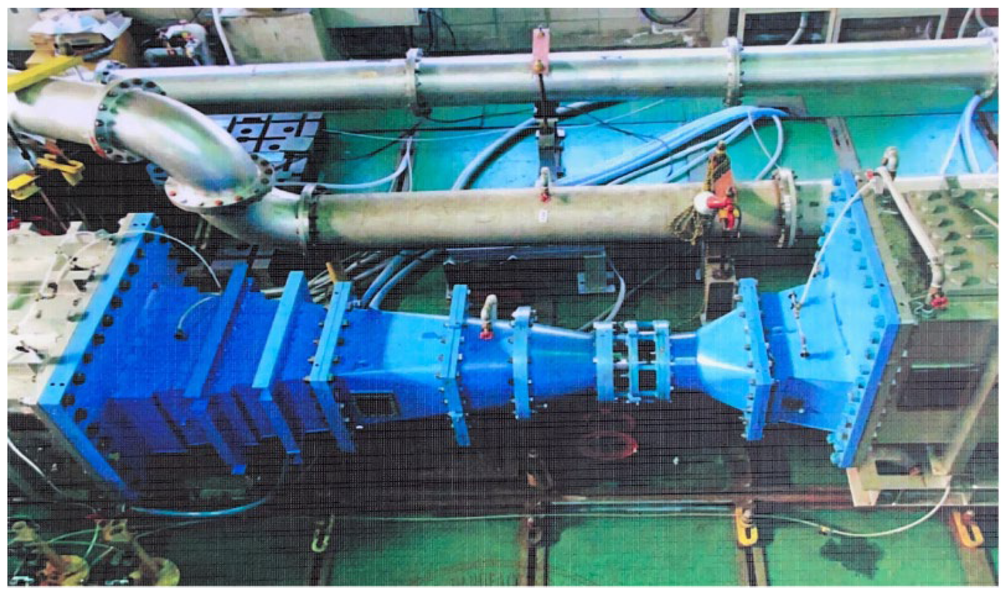
3.1. Experimental Device

In order to verify the accuracy of the numerical simulation, the transient external characteristics of the pumping station model are measured by building the bulb tubular pump experimental device system, as shown in Figure 6. In the test, the rotating speed of the model pump is measured by an electromagnetic tachometer. The measurement error of the instrument is less than 0.1%. The discharge of the model device is measured by an electrical flowmeter, and the error is controlled below ±0.15%, the same as the error of the torque measuring device. Hereinafter, the relevant data are processed by a Computer-Aided Measurement System (CAM). According to the complexity of adjusting the speed of the model pump and collecting relevant calculation data during operation, the accuracy of numerical simulation, by comparing the correlation between the steady numerical simulation of the model pump and the external characteristic curve of the experimental simulation under the rotating speed of 1223 r/min, can be verified. The subsequent analysis is carried out through the numerical simulation data.

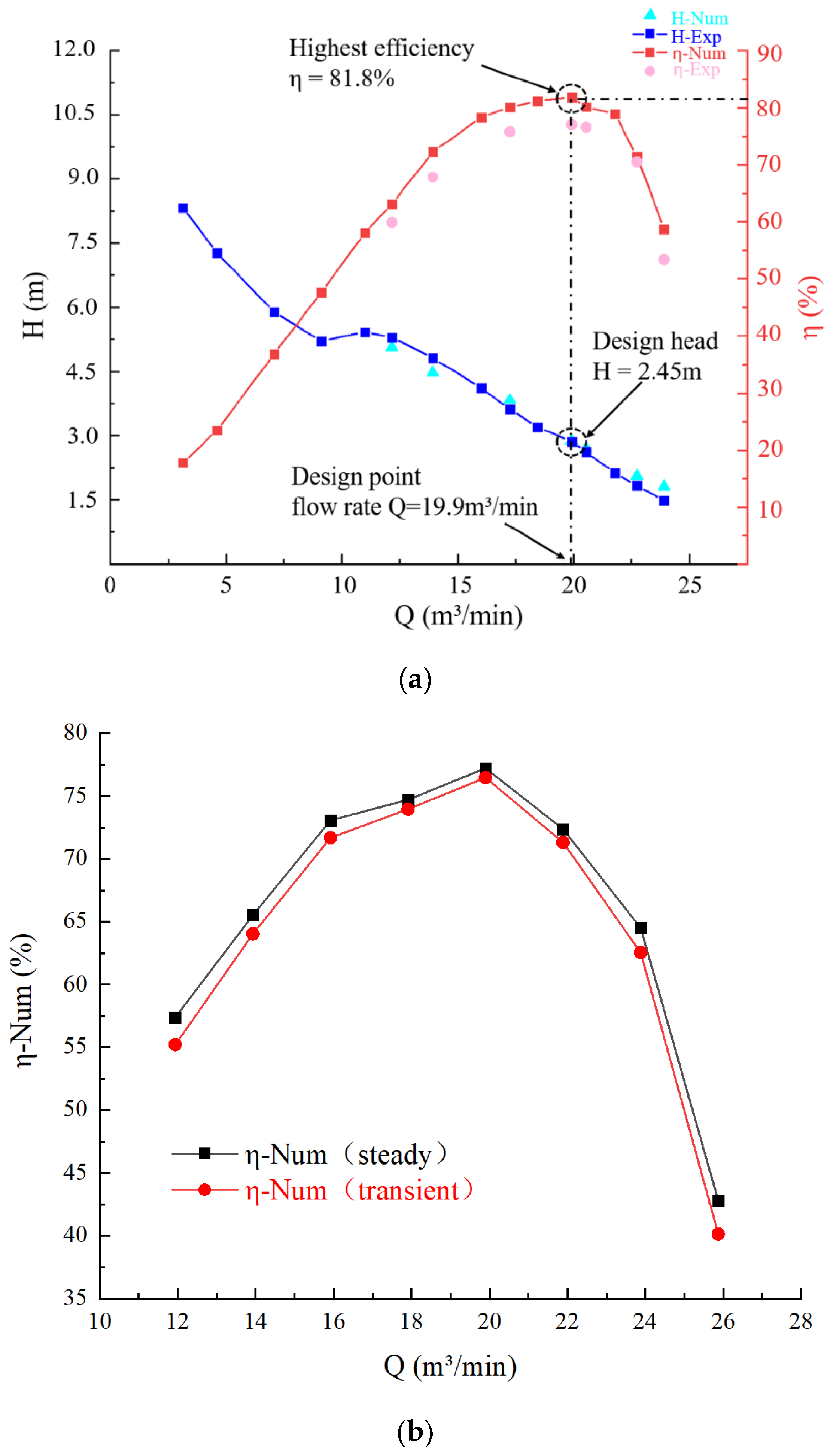
3.2. Comparison of External Characteristic Curves

Some of the external characteristic curves of the pump are obtained through the model test, and they are compared with the results of the numerical simulation to verify the accuracy and reliability of the subsequent numerical simulation of the pump during the deceleration process. As shown in Figure 7a, the head and efficiency under different flow rates calculated by steady numerical simulation with no cavitation are highly consistent with those achieved by the model test, and the error is small. Considering that the subsequent calculations for deceleration are transient simulations, Figure 7b compares the efficiencies obtained from steady and transient numerical simulation. It can be seen that the two efficiency curves maintain a high degree of consistency. Overall, the investigation of the characteristics of the tubular pump during the deceleration process is reliable using the method of transient numerical simulation.

4. Results and Discussion

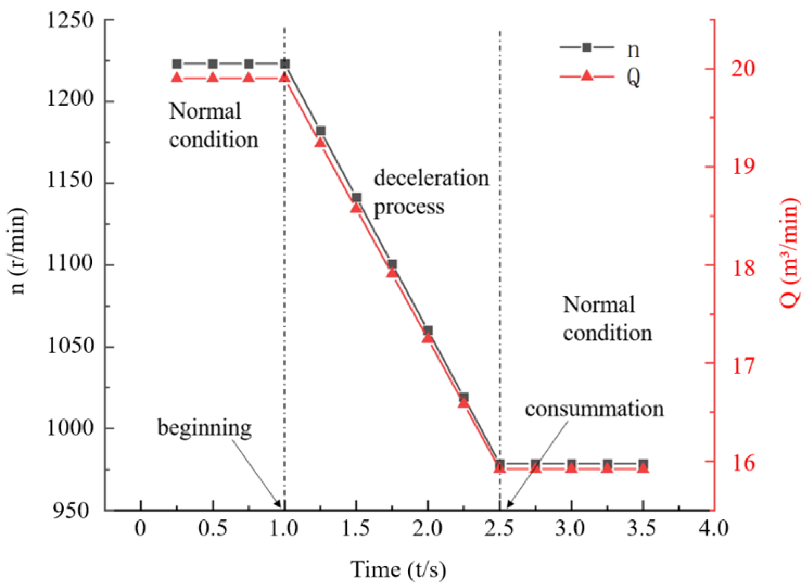
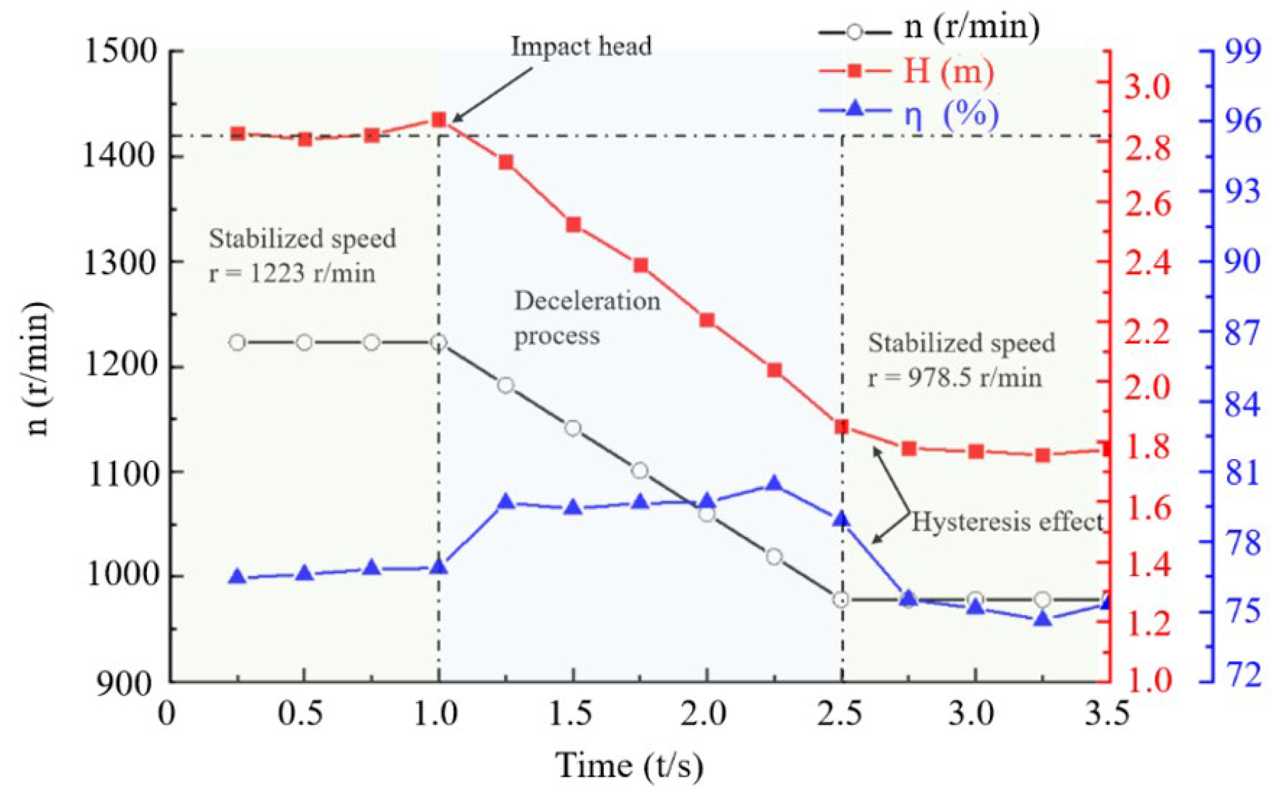
4.1. Transient External Characteristics of CFD

The transient external characteristic curve of the numerical simulation of the model pump unit during deceleration is shown in Figure 8. The three curves changing with time are pump rotating speed, unit head (the difference between inlet and outlet section pressures), and unit efficiency (the full flow field). It can be seen from the figure that the change in head curve maintains the same trend with the rotating speed. When the model pump runs at 0–1 s, the rotating speed in the rotation domain remains stable. At this period, the head of the model pump is stable at about 2.8 m, and the efficiency is stable at 76%. However, at the beginning of the speed change (1 s), the head curve has an obvious impact phenomenon, and its value is about 2% of the head when the rotating speed is constant at 1223 r/min. This is mainly because, under the transient numerical simulation, the fluid is affected by the inertial force. It can be considered that the pump performance curve does not change at this time; however, the inlet flow begins to decrease, so there is a certain impact head phenomenon; in the 1–2.5 s operation of the model pump, the head of the model pump decreases linearly with the decrease in rotating speed, while the efficiency of the model pump remains stable after increasing to 79% in 0.25 s, an improvement of about 3 percentage points. Starting from the 2.5 s of the model pump operation, the rotating speed of the rotation domain is stable at 987.5 r/min. At this stage, the head and efficiency calculated by CFD are affected by the fluid inertia, resulting in an obvious hysteresis effect, and stabilizes at about 1.77 m and 75% when the time reaches 2.75 s.

4.2. Analysis of Internal Flow Characteristics

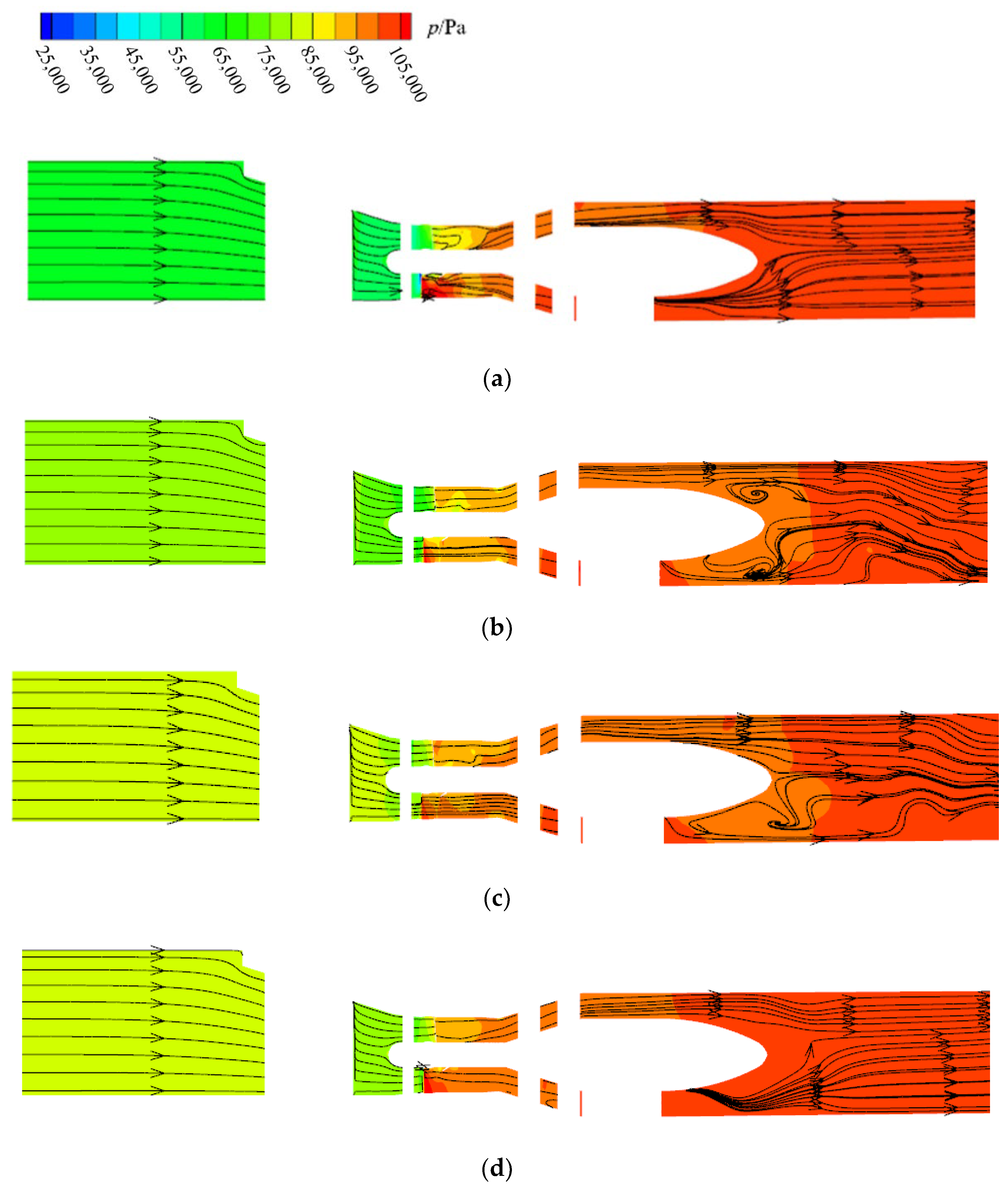
4.2.1. Internal Flow Characteristics in Horizontal Plane

In order to analyze the transient flow field of the tubular pump model in the process of speed change, as shown in Figure 9, the streamline distribution and pressure contours in the horizontal plane of the computational domain at the times of 0.5 s, 1. 5 s, 2.0 s, and 3.0 s are plotted. At 0.5 s, when the rotating speed is stable at 1223 r/min (Figure 9a), the streamlines in the horizontal plane of the entire computational domain are relatively smooth. The pressure distribution of the inlet conduit and the outlet conduit section is relatively uniform, only a comparatively low pressure area appears in the front part of the bulb body, and its value is about 950 kPa. After the water flow is pressurized by the impeller, the pressure distribution of the outlet conduit is obviously larger than that of the inlet conduit. In the process of the rotating speed deceleration (Figure 9b,c), the streamline in the horizontal plane of the water outlet conduit begins to become disordered, and there are turbulence and backflow vortex phenomena at the rear end of the bulb body. The pressure in the inlet conduit begins to increase with time, but the pressure distribution is still uniform, and the comparatively low pressure area in the outlet conduit spreads to about 0.2 m behind the bulb body. After the deceleration is completed (Figure 9d), the streamline in the horizontal plane of the outlet conduit tends to be stable again, but there is still a small amount of vortex and backflow at the rear end of the bulb body, which causes the efficiency reduction shown in Figure 8. The pressure distribution of the outlet conduit is more uniform than that during the rotating speed deceleration, and the comparatively small pressure distribution area is also concentrated only in the front part of the bulb body.

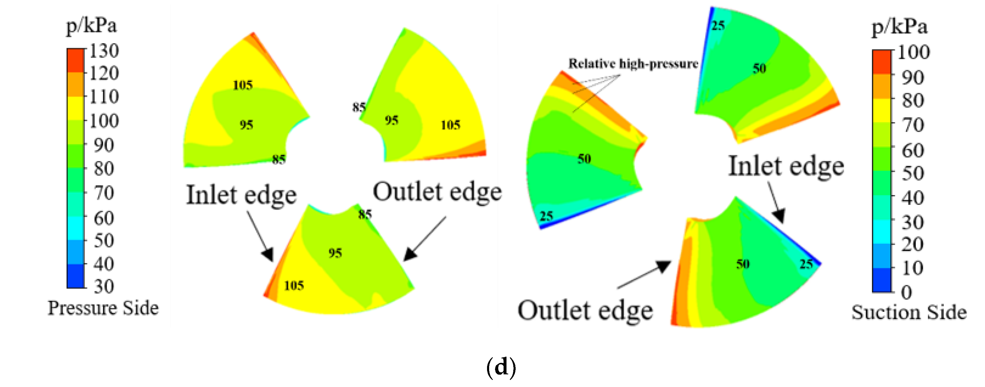
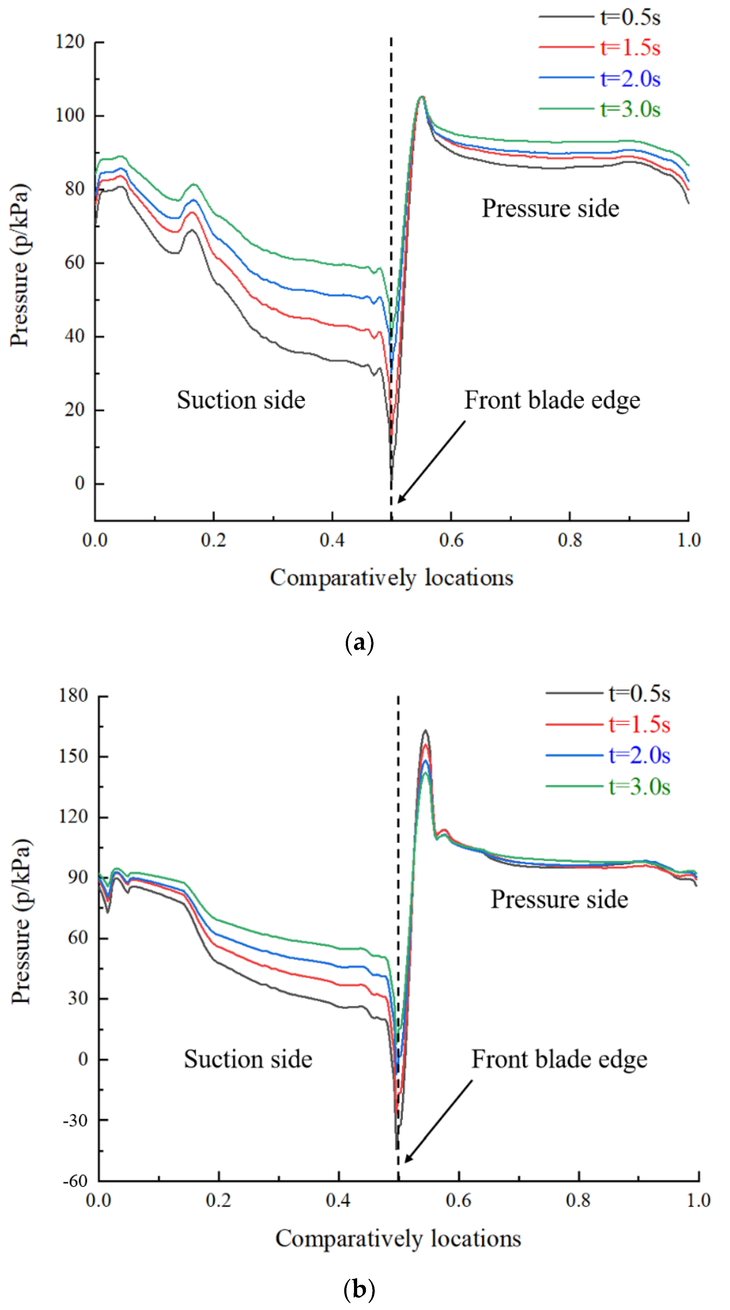
4.2.2. Pressure Distribution of Impeller

Figure 10 shows the transient pressure distribution contours of the impeller blades at different times. At the time of 0.5 s when the speed is stable at 1223 r/min (Figure 10a), it can be clearly observed that comparatively high pressure is generated on the water inlet edge of the impeller blade pressure side due to the impact of the flow, and the comparatively low pressure is distributed from the hub to the outlet edge of the impeller blades. The pressure side of the entire blade basically shows a trend of slow decline in pressure from the water inlet edge to the outlet edge, but the pressure area distribution is irregular. At the same time, the suction side of the blades shows an obvious pressure stratification: on the water inlet edge of the suction surface, a local negative pressure is generated due to the off-flow. Meanwhile, the pressure distribution on the suction side changes uniformly. The pressure areas of 25 kPa, 35 kPa, and 45 kPa are evenly distributed in the middle of the blade, and the area is about 25% of the entire suction surface. The flow forms a comparatively high pressure area on the water outlet edge of the blade again. In the transition process of the speed change (Figure 10b,c), the pressure value and distribution on the pressure surface of the impeller blade do not change obviously; only the comparatively low pressure area on the water outlet edge and the comparatively high pressure area on the water inlet edge are reduced. On the suction side of the blade, although the pressure value still shows a trend of increasing along the flow direction and the stratification phenomenon is obvious, the pressure of about 50 kPa and the comparatively high pressure area increase significantly. Those pressure areas are about 40% to 60% of the entire suction surface. At 3.0 s after the completion of the speed change (Figure 10d), the area of the comparatively high pressure on the water inlet edge and the comparatively low pressure on the water outlet edge of the suction side are reduced to a minimum. In addition, the pressure of about 50 kPa on the suction surface spreads to about 70% of the entire blade, and the comparatively high pressure area also increases to a maximum.

In order to show the characteristics of pressure variation along the flow direction on the blade more clearly, three span lines are made along the direction of the hub to the rim, as shown in Figure 11. The pressure distributions at different times on different span lines are drawn in Figure 12. The X-axis represents the comparative locations on the blade, and the Y-axis represents the pressure values corresponding to the comparative locations. It can be obviously observed that the pressure on the blade surfaces present the trend of uniform increase during the process of deceleration. On the two span lines near the middle of the blades and the rim (span 0.5 and span 0.9), the pressure change mainly occurs on the suction side and the inlet edge of the pressure side of the blade, while the pressure near the hub (span 0.5) shows an obvious numerical change on the entire blade surface except the inlet edge of the pressure side.

4.3. Pressure Fluctuation

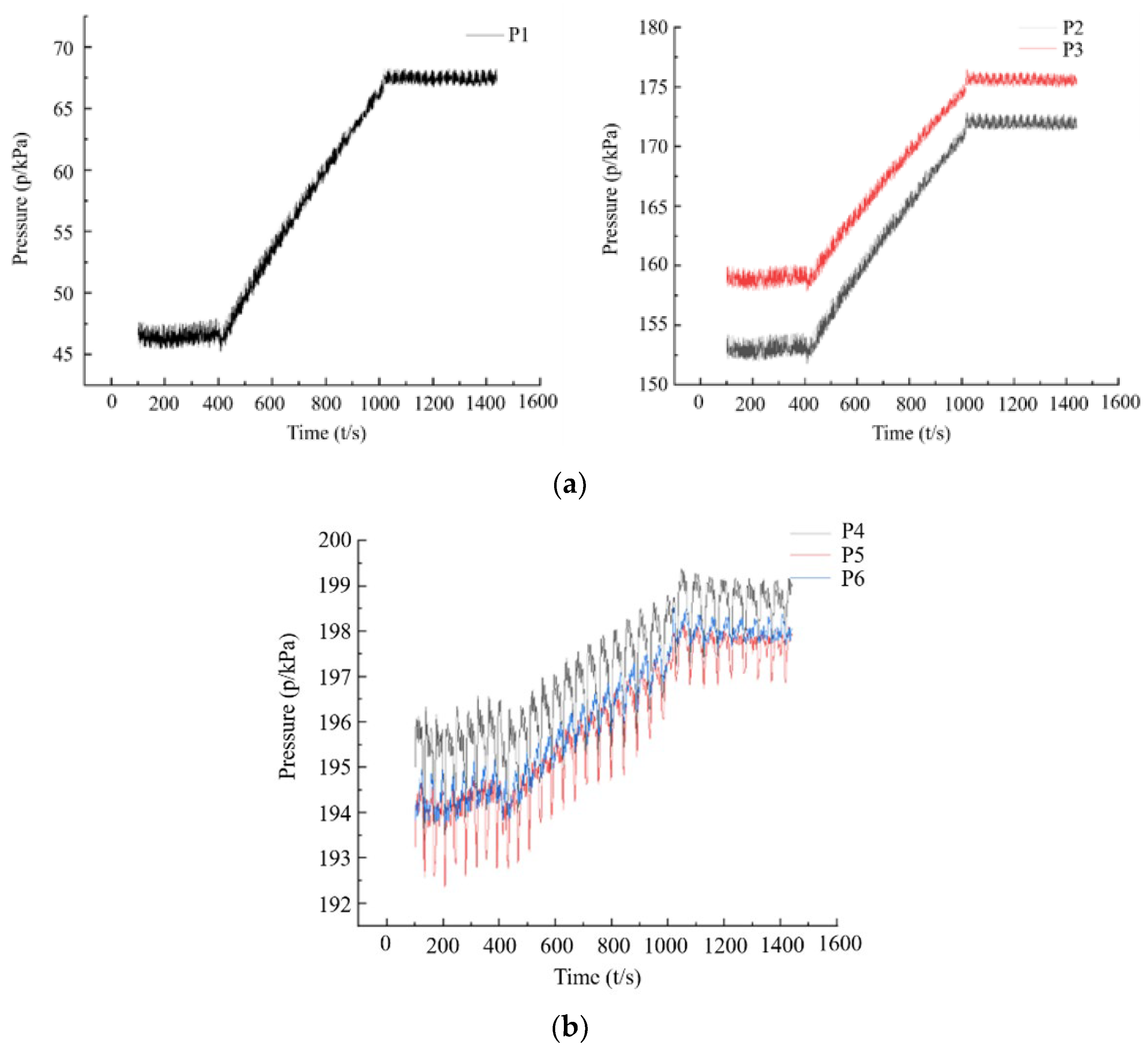
4.3.1. Time Domain Analysis

In order to monitor the pressure fluctuation in the flow field, two monitoring surfaces are set at the front of impeller and the rear of guide vane. In order to capture the influence of radius, three monitoring points are set at the different radii (near the hub, medium radium, and near the rim) of the same monitoring surfaces as those shown in Figure 13.

Figure 14 illustrates the pressure fluctuation time-domain diagram of different monitoring points shown in Figure 13. It can be seen from the figure that the pressure of each monitoring point is quite different from each other: the pressure of the monitoring point at the rim on the impeller inlet section (P1) is smallest, and it increases from 47 kPa to 68 kPa with the deceleration of rotating speed. The closer to the hub, the larger the pressure, but this change decreases as the radius decreases. The pressure of the P3 monitoring point near the hub increases from 157 kPa to 176 kPa with the deceleration of rotating speed. The outlet section of the guide vane also follows the above laws, but the variation is smaller. The data of the two pressure fluctuation monitoring points near the hub are very close, rising from 194 kPa to 197.5 kPa. From the waveform point of view, the pressure fluctuation of the impeller inlet section and guide vane outlet section presents a regular sine or cosine wave, and there are five wave peaks and five wave troughs in a cycle, which is related to the number of blades and guide vanes in the calculation model.

From the overall trend, in the decreasing process, the pressure fluctuation changes of the monitoring points on the two sections are consistent: with the speed decreasing, the pressure fluctuation value increases linearly, the period becomes larger, and the pressure fluctuation amplitude decreases. However, the pressure change range at the outlet section of the guide vane is only about 18% of that of the corresponding monitoring point at the inlet section of the impeller. When the rotating speed starts to change (1 s), a certain degree of pressure impact appears on two sections [25], while the outlet section of the guide vane also has a certain degree of pressure impact when the change in rotating speed ends (2.5 s). However, compared with the pressure fluctuation when the rotating speed is constant, the value of the impact is comparatively small and can be ignored.

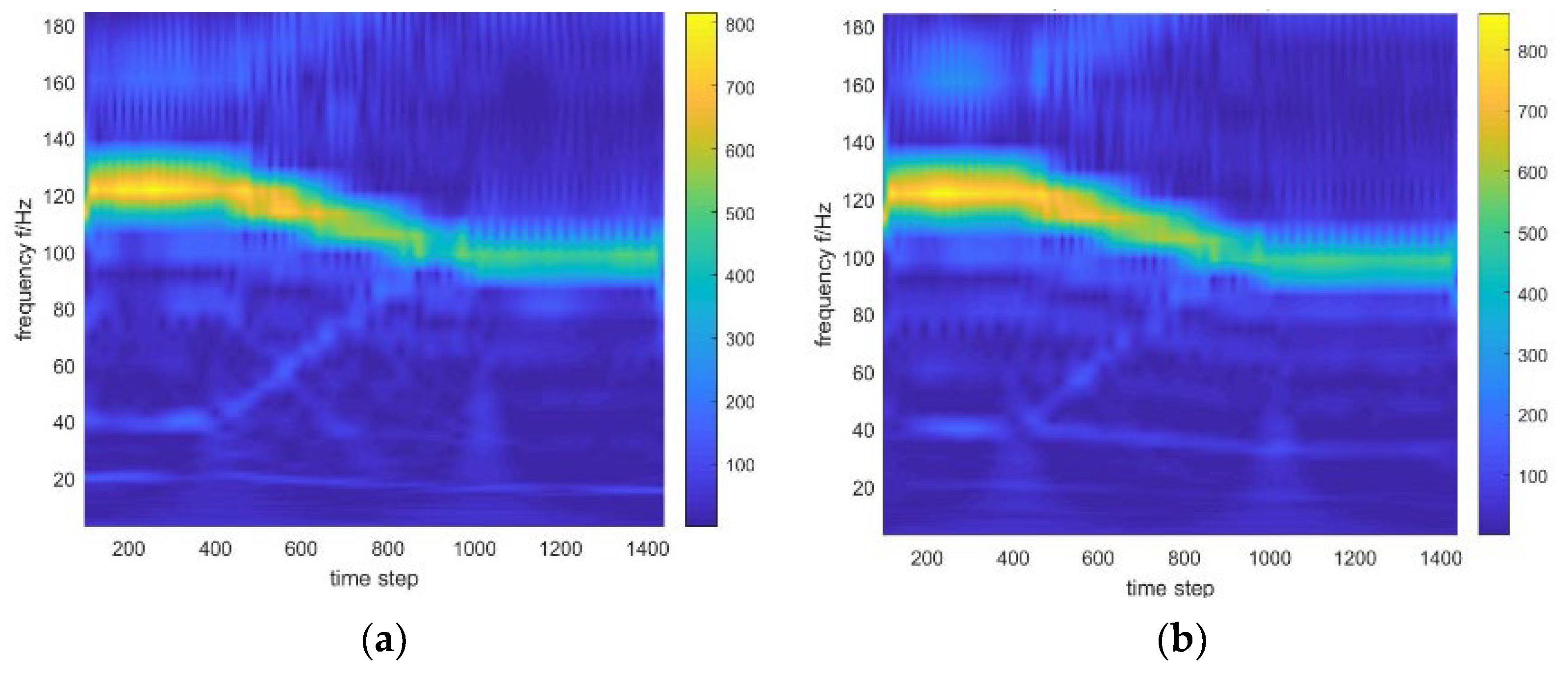
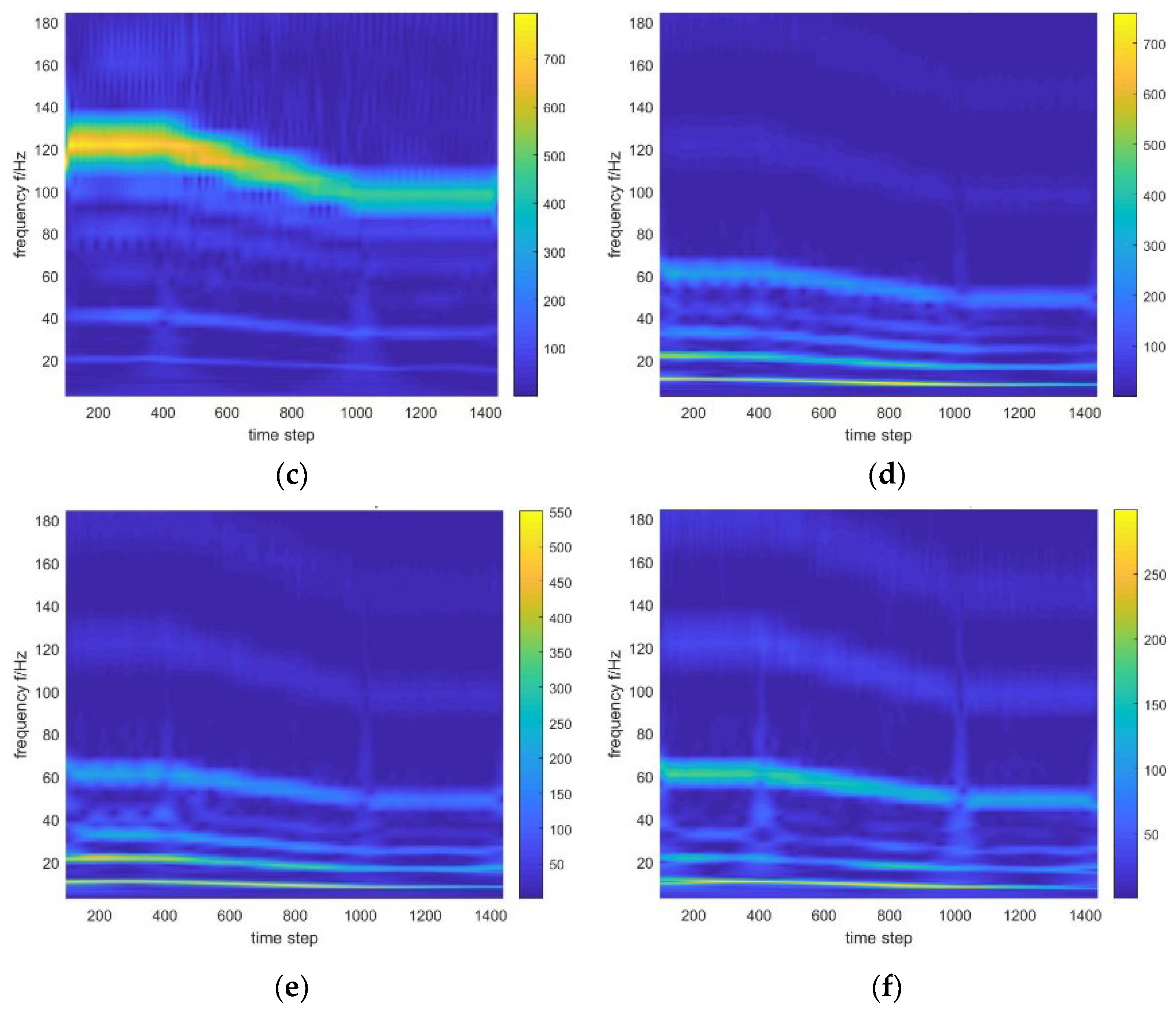
4.3.2. Wavelet Frequency Domain Analysis

As the numerical simulation adopts the linear deceleration method and the number of the impeller blades is 3, the expressions of shaft frequency f_z and blade frequency f are

$$\{\begin{array}{l}{f}_z=\frac{n}{60}\\ f=3f_z\end{array}$$

(3)

where n is the speed of the pump operation stage, r/min. It can be seen from formula (3) that under the design flow condition, the shaft frequency of the bulb tubular model pump is about 20.38 Hz when the rotating speed is 1223 r/min, and the blade frequency is about 61.14 Hz. When the rotating speed is 987.5 r/min, the shaft frequency is about 16.46 Hz and the blade frequency is about 49.38 Hz. The wavelet time–frequency domain conversion is realized by the “cwt” function of MATLAB, and the time–frequency distribution characteristic map of the pressure fluctuation of different sections is drawn as shown in Figure 15, where the abscissa represents the number of time steps, the ordinate represents the fluctuation frequency, and the color represents the fluctuation amplitude. It can be clearly seen from the figure that the main frequency of pressure fluctuation at the inlet section of the impeller decreases linearly from about 122 Hz to about 100 Hz during the deceleration. It can be found that the calculated values of fluctuation frequency are twice the theoretical values of blade frequency calculated by Equation (3), which is due to the influence of the impeller front support vanes [26]. Meanwhile, the fluctuation amplitude before and after the deceleration is also reduced linearly by about 50%, which is basically in line with the analysis above; the pressure fluctuation energy at the outlet section of the guide vane is mainly concentrated in the low-frequency region of 20 Hz and 10 Hz, and the frequency and amplitude change of the fluctuation before and after the deceleration are not obvious, which is mainly affected by the dynamic and static interference of the impeller and guide vanes. It can be seen from the above analysis that the frequency and amplitude of pressure fluctuation are proportional to the rotating speed, and the frequency characteristics of pressure fluctuation on different sections have obvious differences: the fluctuation in the impeller inlet section is mainly concentrated in the high-frequency region, which is sensitive to the change in rotating speed. The pressure fluctuation of the guide vane outlet section is mainly concentrated in the low-frequency region, and it is not sensitive to the change in rotating speed.

5. Conclusions

In this paper, the characteristics of the internal and external flow field and the pressure fluctuation of the bulb tubular pump unit during the deceleration are extracted by numerical simulations. The time–frequency domain analysis method based on wavelets is used to investigate the pressure fluctuation obtained. The results provide a certain reference for the energy utilization and safe operation of the water pump unit in adjusting speeds with variable frequency.

(1)

The predicted head and efficiency of the pump unit based on the numerical simulation are basically consistent with the experimental results, indicating the reliability of the CFD method. The predicted head curve of the bulb tubular pump based on the unsteady flow field calculation maintains a linear downward trend in the process of deceleration, and there is an impact head phenomenon when the speed begins to change, which is about 2% of the value under the speed of 1223 r/min. The predicted efficiency curve maintains a relatively stable high efficiency in the process of speed reduction, and the efficiency is increased by about 3% compared with the stable condition before the speed change. The two prediction curves have a hysteresis effect of about 0.25 s at the end of the speed change.

(2)

In the process of frequency conversion and deceleration of the tubular pump, the pressure distribution on the suction surface of the impeller blade has obvious differences, while this change on the pressure surface is less prominent. At the same time, in the transition process of deceleration, the pressure distribution on the impeller blades is a regular transition, and there is no sudden change or other characteristics.

(3)

From the time-domain analysis of pressure fluctuation, it can be seen that the pressure on the impeller inlet section is sensitive to the change in radius, and the smaller the radius, the smaller the pressure change. Meanwhile, the pressure on the guide vane outlet section is less responsive to the change in radius. With the decrease in rotating speed, the pressure values on the impeller inlet and guide vane outlet sections show a linear upward trend, but the change range of the guide vane outlet section is only about 18% of that on the impeller inlet section. The pressure fluctuation of the two sections has a pressure impact phenomenon at the beginning of the speed change, but the value is small.

(4)

From the frequency domain analysis of pressure fluctuation, it can be seen that the impeller inlet section can better reflect the basic characteristics and changing trend of the fluctuation signal than the guide vane outlet section: the pressure fluctuation energy on the impeller inlet section is mainly concentrated in the high-frequency region. Before and after the deceleration, the main frequencies of the fluctuation are 122 Hz and 100 Hz, which are twice the theoretical rotation frequency of 1223 r/min and 987.5 r/min, respectively, showing an obvious linear decreasing trend in the frequency domain characteristic map. Meanwhile, the amplitude of the pressure fluctuation also increases with the pressure fluctuation energy. The energy on the outlet section of the guide vane is mainly concentrated at about 20 Hz and 10 Hz, the difference between the frequencies is not obvious, due to the dynamic and static interference of the impeller and guide vane, and the change in the speed has less of an effect on the fluctuation amplitude.

References

1. Li, Z. Numerical Simulation and Experimental Study of the Internal Flow in Axial-Flow Pump; Jiangsu University: Zhenjiang, China, 2007. [Google Scholar]
2. Zhu, H.; Zhang, R. Numerical Simulation of Internal Flow and Performance Prediction of Tubular Pump with Adjustable Guide Vanes. Adv. Mech. Eng. 2014, 6, 171504. [Google Scholar] [CrossRef]
3. Xu, X.M.; Lu, Y.J.; Peng, Z.G.; Lu, W. Discussion on the characteristics and selection of large and medium-sized horizontal pump units. Jiangsu Water Resour. 2016, 2016, 20–24. [Google Scholar]
4. Liu, C. Researches and Developments of Axial Flow Pump System. Trans. Chin. Soc. Agric. Mach. 2011, 46, 49–59. [Google Scholar]
5. Li, C.X. Study on Bulb Tubular Pump’s Transient Process with VFD; Yangzhou University: Yangzhou, China, 2011. [Google Scholar]
6. Gu, Y.D.; Li, J.X.; Wang, P.; Cheng, L.; Qiu, Y.; Wang, C.; Si, Q. An Improved One-Dimensional Flow Model for Side Chambers of Centrifugal Pumps Considering the Blade Slip Factor. J. Fluids Eng. 2022, 144, 91207. [Google Scholar] [CrossRef]
7. Gu, Y.; Pei, J.; Yuan, S.; Zhang, J. A Pressure Model for Open Rotor–Stator Cavities: An Application to an Adjustable-Speed Centrifugal Pump with Experimental Validation. J. Fluids Eng. 2020, 142, 101301. [Google Scholar] [CrossRef]
8. Song, X.J.; Liu, C.; Wang, Z.W. Prediction on the pressure pulsation induced by the free surface vortex based on experimental investigation and Biot-Savart Law. Ocean Eng. 2022, 250, 110934. [Google Scholar] [CrossRef]
9. Kan, K.; Zheng, Y.; Chen, H.; Zhou, D.; Dai, J.; Binama, M.; Yu, A. Numerical simulation of transient flow in a shaft extension tubular pump unit during runaway process caused by power failure. Renew. Energy 2020, 154, 1153–1164. [Google Scholar] [CrossRef]
10. Shi, L.; Zhang, W.; Jiao, H.; Tang, F.; Wang, L.; Sun, D.; Shi, W. Numerical simulation and experimental study on the comparison of the hydraulic characteristics of an axial-flow pump and a full tubular pump. Renew. Energy 2020, 153, 1455–1464. [Google Scholar] [CrossRef]
11. Shi, L.; Zhu, J.; Tang, F.; Wang, C. Multi-Disciplinary Optimization Design of Axial-Flow Pump Impellers Based on the Approximation Model. Energies 2020, 13, 779. [Google Scholar] [CrossRef] [Green Version]
12. Yang, Y.; Zhou, L.; Bai, L.; Xu, H.; Lv, W.; Shi, W.; Wang, H. Numerical Investigation of Tip Clearance Effects on the Performance and Flow Pattern Within a Sewage Pump. J. Fluids Eng. 2022, 144, 81202. [Google Scholar] [CrossRef]
13. Liu, J.; Liu, S.; Wu, Y.; Jiao, L.; Wang, L.; Sun, Y. Numerical investigation of the hump characteristic of a pump–turbine based on an improved cavitation model. Comput. Fluids 2012, 68, 105–111. [Google Scholar] [CrossRef]
14. Pesch, A.; Melzer, S.; Schepeler, S.; Kalkkuhl, T.; Skoda, R. Pressure and Flow Rate Fluctuations in Single- and Two-Blade Pumps. J. Fluids Eng. 2020, 143, 11203. [Google Scholar] [CrossRef]
15. Song, X.-J.; Yao, R.; Chao, L.; Wang, Z.-W. Study of the formation and dynamic characteristics of the vortex in the pump sump by CFD and experiment. J. Hydrodyn. 2021, 33, 1202–1215. [Google Scholar] [CrossRef]
16. Song, X.; Luo, Y.; Wang, Z. Numerical prediction of the influence of free surface vortex air-entrainment on pump unit performance. Ocean Eng. 2022, 256, 111503. [Google Scholar] [CrossRef]
17. Tsukamoto, H.; Matsunaga, S.; Yoneda, H.; Hata, S. Transient Characteristics of a Centrifugal Pump During Stopping Period. J. Fluids Eng. 1986, 108, 392–399. [Google Scholar] [CrossRef]
18. Liu, J.; Li, Z.; Wang, L.; Jiao, L. Numerical Simulation of the Transient Flow in a Radial Flow Pump during Stopping Period. J. Fluids Eng. 2011, 133, 111101. [Google Scholar] [CrossRef]
19. Chalghoum, I.; Elaoud, S.; Akrout, M.; Taieb, E.H. Transient behavior of a centrifugal pump during starting period. Appl. Acoust. 2016, 109, 82–89. [Google Scholar] [CrossRef]
20. Zhang, R.T.; Yao, L.B.; Zhu, H.G.; Zhang, L.; Wei, J. Low-head pumping system performances and affinity issues under variable speed operation based on CFD. J. Drain. Irrig. Mach. Eng. 2010, 28, 5. [Google Scholar]
21. Cheng, J.L.; Zhang, R.T.; Deng, D.S.; Yi, D.; Xusong, F. Adaptability research of optimal operation mode with variable frequency drives for pumping stations in China’s Eastern Route Project of S-to-N Water Diversion. J. Drain. Irrig. Mach. Eng. 2010, 28, 5. [Google Scholar]
22. Li, W.; Ji, L.L.; Shi, W.D.; Zhang, Y.; Zhou, L. Numerical Calculation of Internal Flow Field in Mixed-flow Pump with Non-uniform Tip Clearance. Trans. Chin. Soc. Agric. Mach. 2016, 47, 66–72. [Google Scholar]
23. Yang, L.; Xu, Z.; Zhen, Y. Study on shutdown transition process of large low head pumping station. Water Conserv. Constr. Manag. 2020, 40, 73–79. [Google Scholar]
24. Zhang, F. Application of Wavelet on Status Monitoring and Failure Diagnosis of Large Scale and Intermediate Pump Unit. Master’s Thesis, Hohai University, Nanjing, China, 2007. [Google Scholar]
25. Li, W.; Lu, D.L.; Ma, L.L.; Ji, L.; Wu, P. Experimental study on pressure vibration characteristics of mixed-flow pump during start-up. Trans. Chin. Soc. Agric. Eng. 2021, 37, 44–50. [Google Scholar]
26. Shi, W.; Cai, R.M.; Li, S.B.; Sun, T.; Shen, C.; Cheng, L.; Luo, C. Numerical simulation of pressure fluctuation in postpositional bulb tubular pump. South North Water Transf. Water Sci. Technol. 2021, 37, 44–50. [Google Scholar]
Figure 1. 3D model of horizontal bulb tubular pump.
Water 14 01788 g001
Figure 2. Grid of impeller domain.
Water 14 01788 g002
Figure 3. Hydraulic losses under different grid numbers.
Water 14 01788 g003
Figure 4. Grid of full channel calculation domain.
Water 14 01788 g004
Figure 5. Impeller speed and flow inlet change.
Water 14 01788 g005
Figure 6. Experimental setup.
Water 14 01788 g006
Figure 7. Comparison of numerical simulation and experimental results: (a) Steady numerical simulation and experimental results; (b) Steady and transient numerical simulation results.
Water 14 01788 g007
Figure 8. Transient external characteristic curve.
Water 14 01788 g008
Figure 9. Streamline and pressure contours in horizontal plane of the pump at different times: (a) t = 0.5 s; (b) t = 1.5 s; (c) t = 2.0 s; (d) t = 3.0 s.
Water 14 01788 g009
Figure 10. Pressure distribution contours of the pump impeller blades at different times: (a) t = 0.5 s; (b) t = 1.5 s; (c) t = 2.0 s; (d) t = 3.0 s.
Water 14 01788 g010aWater 14 01788 g010b
Figure 11. Schematic diagram of the different span line positions.
Water 14 01788 g011
Figure 12. Pressure characteristics at different span lines under deceleration: (a) span = 0.1; (b) span = 0.5; (c) span = 0.9.
Water 14 01788 g012aWater 14 01788 g012b
Figure 13. Pressure fluctuation monitoring points.
Water 14 01788 g013
Figure 14. Pressure characteristics of sections: (a) impeller inlet section; (b) guide vane outlet section.
Water 14 01788 g014
Figure 15. Frequency distribution of pressure fluctuation under two sections: (a) monitoring point P1 on the impeller inlet section; (b) monitoring point P2 on the impeller inlet section; (c) monitoring point P3 on the impeller inlet section; (d) monitoring point P4 on the guide vane outlet section; (e) monitoring point P5 on the guide vane outlet section; (f) monitoring point P6 on the guide vane outlet section.
Water 14 01788 g015aWater 14 01788 g015b