
Laboratory Studies on the Parametrization Scheme of the Melting Rate of Ice–Air and Ice–Water Interfaces

1
State Key Laboratory of Coastal and Offshore Engineering, Dalian University of Technology, Dalian 116024, China
2
North China Sea Marine Forecasting Center of State Oceanic Administration, Qingdao 266000, China
*
Author to whom correspondence should be addressed.
Water 2022, 14(11), 1775; https://doi.org/10.3390/w14111775
Submission received: 5 May 2022
/
Revised: 26 May 2022
/
Accepted: 29 May 2022
/
Published: 1 June 2022
(This article belongs to the Special Issue Sea, River, Lake Ice Properties and Their Applications in Practices)
Abstract
:During the melt season, surface melting, bottom melting, and lateral melting co-occur in natural ice floes. The bottom melting rate is larger than the lateral melting rate, followed by the surface melting rate, and the smaller the size of an ice floe, the higher the lateral melting rate. To add the scale index of small-scale ice to the melting parametrization scheme, experiments on the melting process of sea ice and artificial fresh-water ice samples in the shape of a disc were carried out in a low-temperature laboratory, under conditions of no radiation, current, or wind, with controlled air and water temperatures. The variations of diameter, thickness, and mass of the ice discs were measured through the experiments. According to the experimental data, a new indicator was created using the ratio of the diameter to the thickness of an ice sample. Based on physical and statistical analyses, the relationships between the surface/bottom melting rates and temperature gradient were formulated. Additionally, the relationships among the lateral melting rate, temperature difference, and the ratio of the diameter to the thickness were also quantified. The equations can be applied to the melting parametrization scheme of ice for a range of diameters up to 100 m, which covers simulations of the energy and mass balance values of the Arctic sea ice and coastal freshwater ice during the summer melt season.
1. Introduction
With global warming, the annual warming trend of the Arctic temperature is 2–3 times that of the global temperature, which is also known as the Arctic amplification effect [1,2,3]. Sea ice changes in the Arctic are not only related to local climate, but also affect climate changes in the mid-latitudes of the Northern Hemisphere, such as by increasing extreme weather events in Eurasia and North America [4,5]. Sea ice models are effective tools to describe the evolution of sea ice which mainly include thermodynamic and dynamic processes [6,7].
In general, ice thickness distribution (ITD) and sea ice concentration are used to describe the state of sea ice in a given area in the sea ice models [8]. The World Meteorological Organization uses floe size (form of ice) in addition to these two terms to describe ice, and uses an egg code as the standard way to describe ice [9]. The floe size distribution (FSD) is also needed in the developments of sea ice models, especially in the simulation of a marginal ice zone (MIZ) [10]. In the empirical formula according to the observations, FSD generally could be represented by a power law [11]. To accurately describe FSD, lateral melting plays an important role in the contribution to the conservation formula of FSD. For example, in the Arctic summer, a rapid melting rate occurs not only in the bottom and surface, but also in the lateral interface between sea ice and ocean, especially in MIZ. The contribution of lateral melting to ice ablation and perimeter increases has a more important role than before, because of floe breaks [12]. The lateral melting rate and perimeter of floes often determine the magnitude of a net heat flux exchanged between the ocean and the lateral edge of sea ice [13]. The melting rate is sensitive to floe size due to the increase in the perimeter of the lateral ice edge when floe size is smaller than 30 m [14]. Due to the decrease in ice extent and thickness, the evolution of sea ice shows new characteristics different from previous cases. For larger floe sizes, the lateral melting of sea ice may also have an important contribution since the ice meltwater fronts accelerate the lateral mixing [15]. An active exploration of the lateral melting mechanism is necessary to understand Arctic sea ice melting during the summer.
Field investigations are important means of understanding the lateral melting physical processes of sea ice. In the programs of Arctic Ice Dynamics Joint Experiment and Marginal Ice Zone Experiment, researchers have investigated the relationship between floe size shape and lead heat flux [14,16]. Hwang et al. (2017) and Perovich and Jones (2014) have observed the evolution of floe size and found that lateral melting plays an important role in the variation of FSD [17,18]. Stern et al. (2018) are continuously conducting observational studies in which the seasonal cycle of the FSD is analyzed and lateral melting contributes quantitatively to the seasonal cycle [19].
At present, only a few field observations of the lateral melting of the Arctic sea ice have been conducted due to the limitations imposed by the polar field conditions and testing techniques. As a result, different techniques and methods were tested on stable lake ice in China and the acquired data were applied to the parametrization research of lateral melting [20,21]. These in situ experiments on lake ice have comprehensively investigated the multifactors of air temperature, solar radiation, and water temperature contributing to the lateral melting, and the limit in understanding the contributions of one particular factor to lateral melting. However, the effect of floe size on the lateral melting is still difficult to observe in in situ experiments due to the lack of effective techniques. In this paper, the laboratory experiments were conducted for the melting on the basal and the lateral interfaces of ice, improving the understanding of the lateral melting process, and then giving a parametrization scheme of the lateral melting rate varied with floe size.
2. Theoretical Foundation
The lateral melting of sea ice depends on the net heat flux from the ocean and atmosphere to lateral ice [22]. The net heat flux generally includes shortwave and longwave radiation, sensible heat flux, conductive heat flux, and latent heat flux [23]. The melting rate contributes to latent heat flux. In the literature (Bateson et al., 2020; Roach et al., 2018) [10,24], the lateral melting rate is expressed in a power law, which is:
where is the lateral melting rate of ice, is the difference of water temperature above the freezing point, and a and b are the statistical parameters based on observations.
Smith et al. (2022) used an equation for the ice surface, bottom, and lateral melting based on the sea ice concentration [25]:
where is the sea ice concentration per unit area and ranges from 0–1, is the surface melting rate of ice, is the bottom melting rate of ice, is the ice thickness, is the floe diameter (300 m in the default set up of sea ice models), and is the geometric parameter representing the deviation of floe with a circular shape ( = 0.66). and contribute to the variation of ice thickness H; and when H keeps constant, and can be neglected, and the equation can be written as:
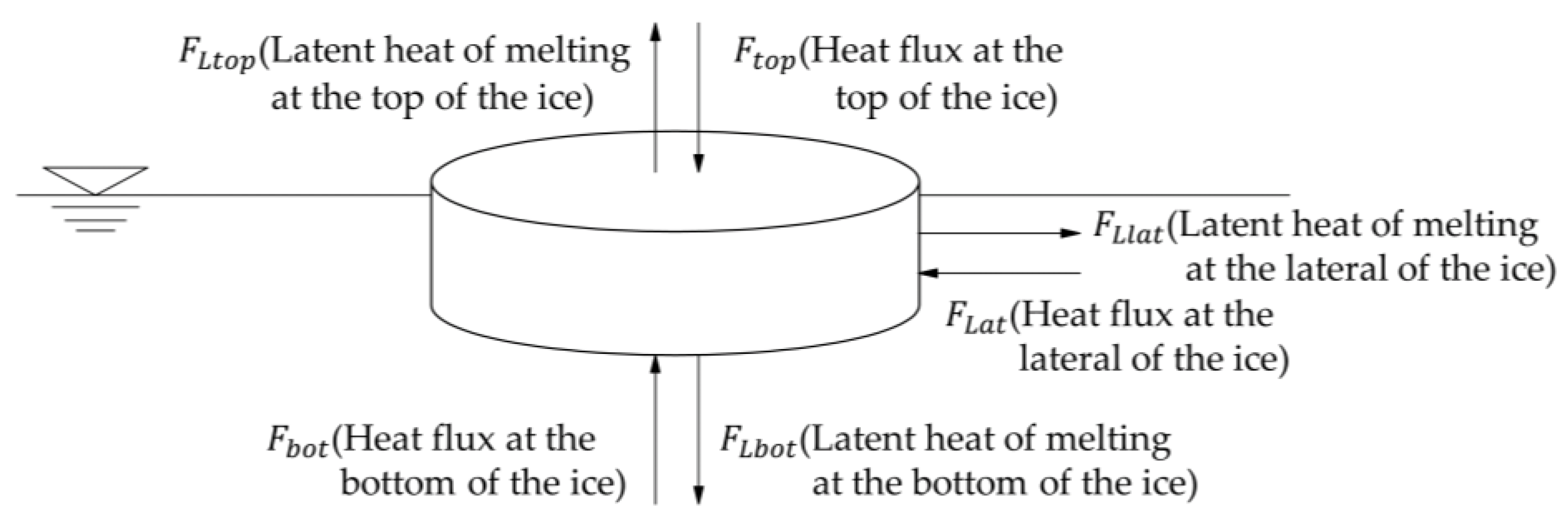
In particular, ice with an equivalent diameter of less than 30 m is thought to be greatly affected by lateral melting [14]. In this paper, ice samples were used in the laboratory to model surface, bottom, and lateral melting of ice. The observed changes in the diameter were the result of the lateral melting on the surface of the samples, whereas the thickness variation data indicated the melting of the surface and the bottom, and the mass variation was an integral demonstration of the three melting processes. The Figure 1 schematic illustrates the heat flux and the thermal balance of the surface, bottom, and lateral interfaces during ice floe melting.
Laboratory experiments are conducted in an ideal condition. As shown in Figure 1, the net heat flux mainly includes two parts. One is the latent heat flux resulting from melting, the other is heat flux from the environment (air or water) to ice. The latent heat flux is proportional to the melting rate, and the other heat flux is proportional to the gradient of temperature. The equation for the surface melting rate is:
The bottom melting rate is given by [26]:
where and are air and water thermal conductivity, respectively; and are the difference of temperatures between air and ice surface, and difference of temperatures between water and ice bottom, respectively; and are references to height and depth according to measurement positions; and L represents the latent heat.
3. Experimental Method
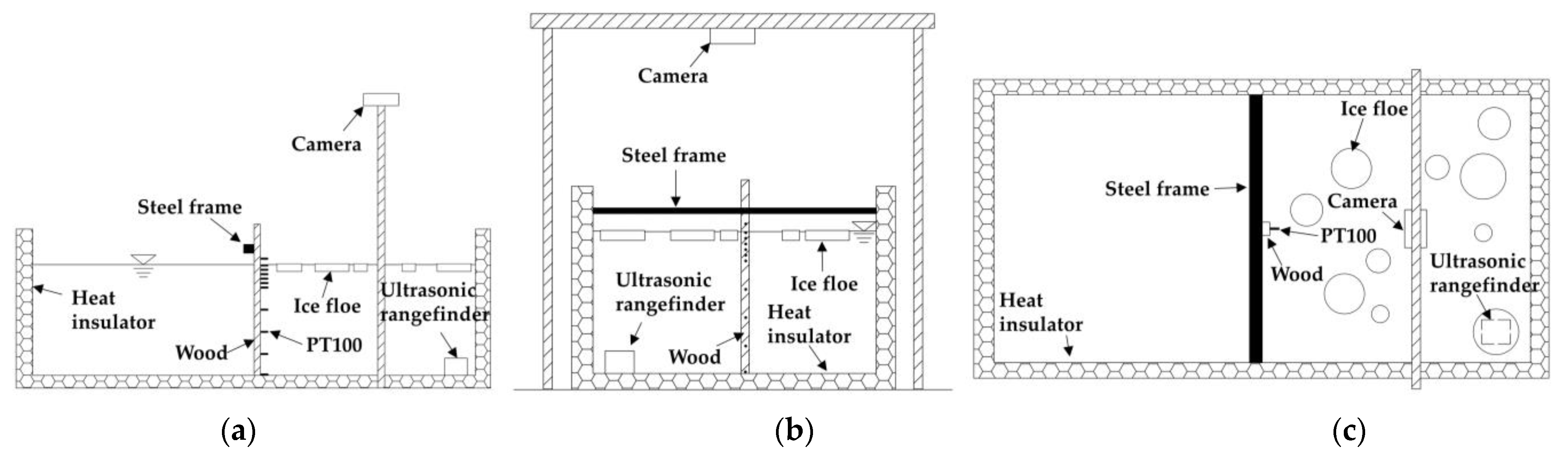
A water tank 2 m long, 1 m wide, and 0.8 m high was set up in the low-temperature laboratory. The tank was designed specially with a double-layer bottom, and a pump was installed at the lower layer to drive the water before tests and was stopped during test. The experimental water tank can hold water to a depth of 0.5 m. A schematic of the laboratory equipment system is shown in Figure 2. The melting process of the ice samples was affected jointly by the temperature of the air above the water tank and the water inside. So, the PT100 temperature probes were distributed along the direction of depth, from the air above the tank to the water in the tank. With a diameter of 5 mm, each temperature probe was precision-corrected in the factory to satisfy a temperature measurement accuracy of 0.1 °C. The air temperature probes were installed above the water surface at a height of 50 cm and 3 cm, respectively. For the water temperature measurements, probes were set up at depths of 0, 2, 4, 6, 8, 10, 20, 30, 40, and 50 cm. To reduce the interference caused by the small probe spacing, the adjacent two temperature probes were inserted vertically into the wood.
A COOLPIX P6000 camera, with 13.5 million pixels, was installed 0.7 m above the water surface at the tank center. Photos taken by the camera had the quality of each pixel corresponding to 0.5 mm × 0.5 mm. An under-ice ultrasonic range finder with high precision (±0.1 mm) was set on the bottom of the water tank. Both the camera and the ultrasonic range finder were used as aid technology in this experiment; that is, the measured data using the camera and ultrasonic range finder were not included into the analysis below but were used to validate the manual measurements during tests. The camera traced the diameter variation on the surface of the ice sample, and the ultrasonic range finder traced the level variation on the bottom of a specific ice sample.
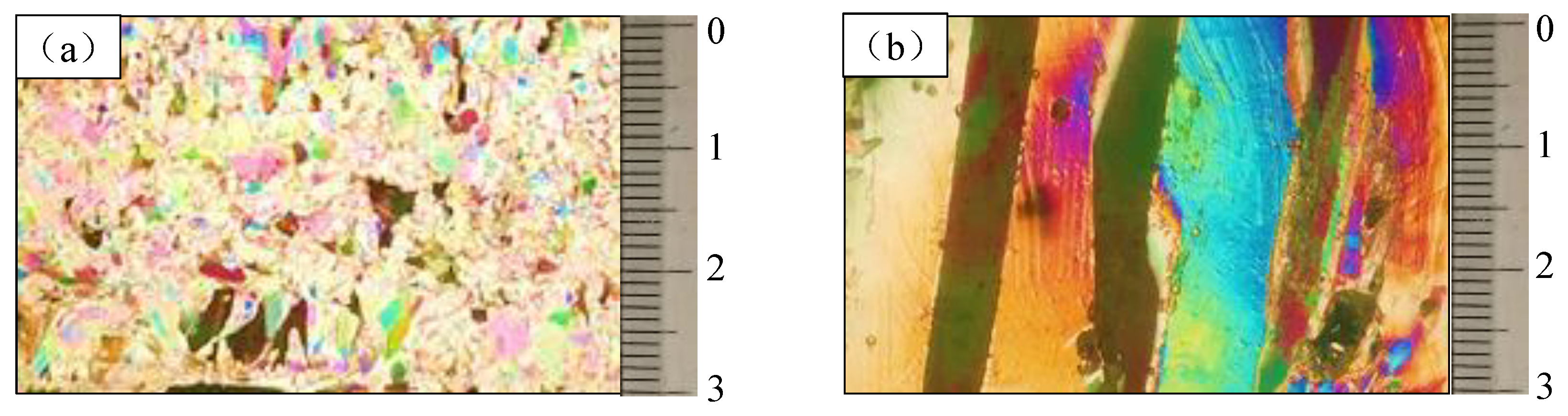
In this experiment, two types of ice samples were used: natural sea ice from the Yellow Sea and artificial fresh-water ice. The sea ice was level ice with a thickness of about 30 mm that had been collected from the Xiajiahezi seashore, Dalian, during 4–6 January 2021, transported to the laboratory directly without large temperature variations and then stored at a low temperature. The sampling site was not far away from the laboratory so that large brine loss would not occur. The sea ice was then cut using a chain saw and lathe to diameters of 65, 90, 120, 150, and 190 mm. For the artificial fresh-water ice, constant temperature technology was used to maintain the lateral water temperature at the freezing point so that the ice would freeze unidirectionally. The unidirectionally frozen ice was processed using a lathe to diameters of 65, 90, 120, 150, and 190 mm, at a thickness of about 30 mm. The sea ice was melted for measuring salinity using a salinometer, and the mean salinity was 6.04 ppt, which is close to the typical salinity of sea ice in the Yellow Sea. The densities of sea ice and fresh-water ice were measured using the mass/volume method, and the mean densities were 800 kg/m3 for sea ice and 900 kg/m3 for fresh-water ice. The ice crystal structure was observed by first preparing 1 cm thick vertical sections using a band saw. These thick sections were attached to glass plates and cut further to an approximately 0.5 mm thickness. These thin sections were placed on a universal stage to observe the crystal structure under crossed polarized light, recorded by photography. Figure 3 shows the two crystal types. The sea ice was granular ice, and the fresh-water ice was columnar ice.
By adjusting the air temperature in the low-temperature laboratory, the water temperature in the water tank was kept stable. In this experiment, the sea water was salty water prepared using sea salt, with a salinity (tested as 27.7 ppt) in accordance with the median value of the ocean salinity profile for the Arctic summer sea ice area, as reported in the literature [27]. The fresh water was tap water. Before the experiment, different preliminary water temperature ranges were set for the sea ice and the fresh-water ice experiments. Based on the temperature-controlling abilities of the laboratory, the water temperatures were set at −0.5, 0, 0.5, 1.0, and 1.5 °C in the sea ice tests and 0.5, 1.5, 2.0, and 3.0 °C in the fresh-water tests. Since the fresh water is simpler in phase composition than sea ice, the temperature groups were less in fresh-water tests and the test temperatures were set higher in fresh-water ice tests than in sea ice tests.
Before each experiment, ice samples were stored in the thermotank at the temperature of 1 °C lower than the freezing point for at least 24 h. When water temperature was measured close to the designed temperature, samples with five different diameters were placed in the water tank at the same time. Samples were labeled with different color stickers or numbers for identification. The variations in the diameter, maximum thickness, and mass of each sample were traced in the test. Both manual measurements and electro-test aided technology were carried out simultaneously during the melting process. At the beginning of each experiment, there was less melting of ice, so the lateral melting, thickness melting, and mass melting were measured directly after the samples were taken out of the water. In general, the measurement interval was set to about 1 h to minimize the influence of the manual testing on the experimental results. The maximum thickness and the surface diameter of the ice samples were measured by an electronic digital caliper (±0.01 mm), and the mass was measured using an electronic scale. The whole process was rapid and the samples were taken with caution so that no wave was produced and the temperatures of air, ice, and water would not be affected. A foam disc with a diameter of 10 cm was placed in the ice sample as a reference for photographing to calibrate the equivalent diameter on the surface of the ice samples at different moments determined using a sample area. Both the camera and ultrasonic sensor were set to record data at an interval of 10 min.
4. Results
Before the experiment, an electronic digital caliper was used to measure the diameter and thickness of each sample three times at different positions, respectively, based on which the average initial values of these two parameters were calculated. The initial size information of the two types of samples is listed in Table 1.
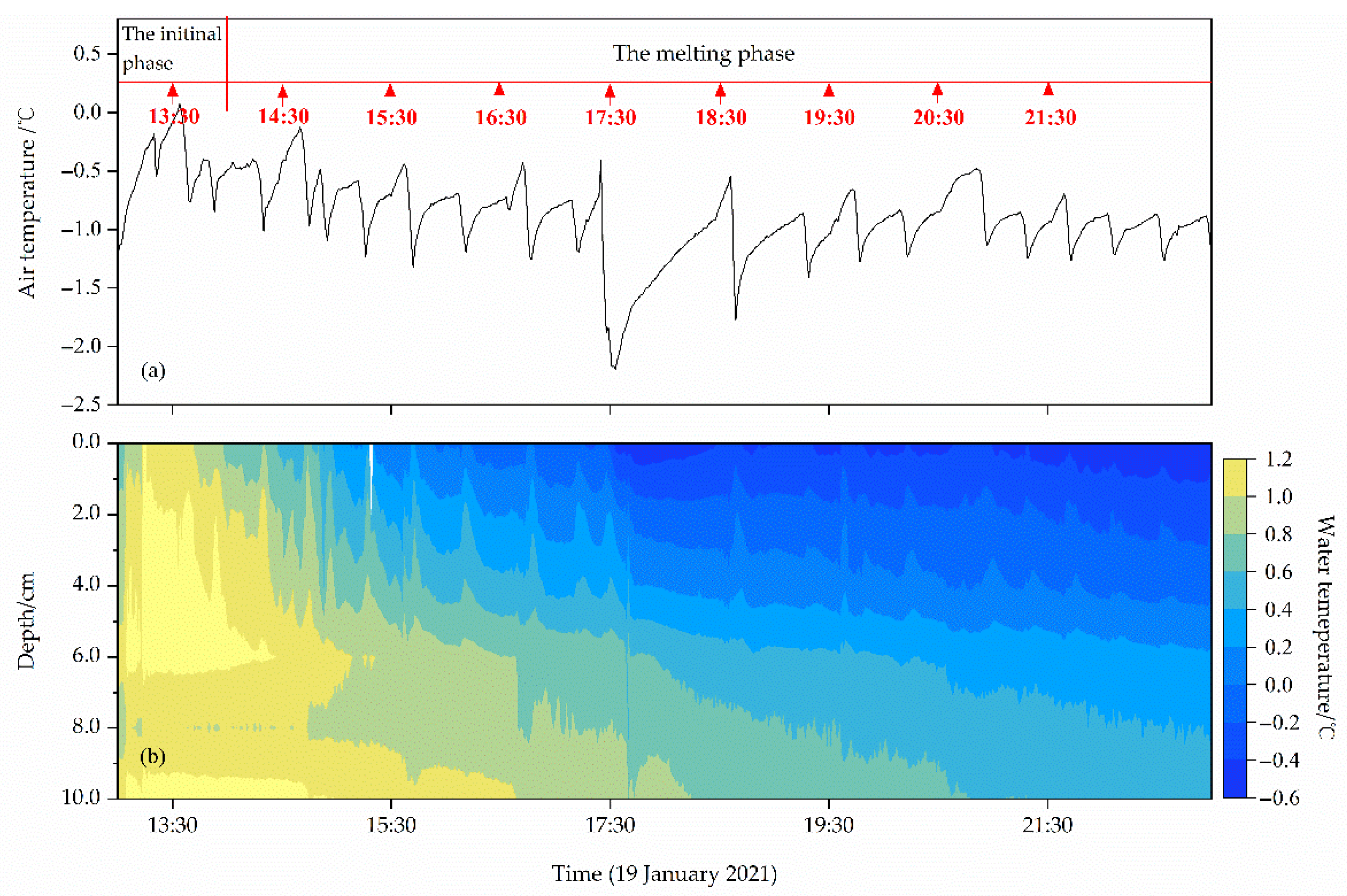
Throughout the experiment, no heat exchange was caused by solar radiation or wind convection in the low-temperature laboratory and only the indoor temperature was used as the driving factor to control the water–ice heat exchange. The designed preliminary water temperature was higher than the experimental water temperature to ensure that lateral and bottom melting occurred after the ice absorbed heat during the whole experiment. The temperature in the low-temperature laboratory was characterized by (1) temperature control fluctuations resulting from the refrigeration system, (2) a temperature increase “pulse” in the daily defrosting of the refrigeration system, and (3) a slight long-term temperature increase. Figure 4a presents the temperature changes at a position of 3 cm above the water surface during the experiment, where a sea ice sample with a designed preliminary water temperature of 1.0 °C is taken as an example.
The experiment was conducted from 13:30 to 21:30 on 19 January. Before the experiment, the water in the tank was stirred constantly to uniformly reduce the water temperature to 1.0 °C. The air temperature at a distance of 3 cm from the water surface was kept below 1.0 °C for a period of time to stabilize the water temperature. Next, the sample was placed into the tank. Thus, the temperature in the laboratory was reduced due to the heat absorption of the ice sample. However, the operation of the refrigerator guaranteed a regular fluctuation of 0.4 °C. Finally, a temperature “pulse” caused by the short-term defrosting was observed at 17:30.
The sample melted after absorbing heat from the water, leading to a temperature reduction from the water surface to the depth of ice immersion. The temperature of the water at the same depth also experienced a decrease with the adjustment of air temperature. However, the vertical temperature gradient of the water under the ice gradually increased with depth, which could be attributed to the heat absorption in the ice-melting process. Taking the sea ice sample with the designed preliminary water temperature of 1.0 °C as an example, Figure 4b records the changes in water temperature, including changes in the section of the example experiment, where the water temperature decreased with the melting of the sample. The water and air temperatures first remained stable and then increased after the ice sample had completely melted.
As seen in Figure 4, large changes occurred in the frequency and amplitude of the air temperature, whereas the water temperature remained stable during the experiment. According to the color gradation diagram of the water temperature in Figure 4b, the water was uniformly stirred before 14:00 and its temperature reached the designed preliminary water temperature of about 1.0 °C, indicated by the yellow color. After all the ice samples were placed in the tank, the surface water temperature reduced quickly, while the temperature of the lower water reduced slowly. Abrupt changes in water temperature were observed before 18:00, and the whole experiment displayed a clear vertical water temperature gradient. Moreover, the temperature of the water from a depth of 2 to 4 cm underwent a higher rate of reduction owing to the ice thickness of 3 cm.
A typical picture of a melting ice sample is shown in Figure 5. The diameter, maximum thickness, and mass changes of the sea ice samples with different diameters with a designed preliminary water temperature of 1.0 °C are shown in Figure 6. The changes in the surface diameter during the ice-melting process are displayed in Figure 6a. The diameter reduced gradually in the initial stage due to the hysteresis of heat absorption. The reduction rate then increased with time. Figure 6b depicts the thickness changes in the samples. As the experiment continued, the sample first melted rapidly and then slowly, eventually reaching a stable state. The melting rates of the samples with different diameters were basically the same. According to Figure 6c, the overall mass of the sample decreased in the experiment. At the beginning, due to the large pores of the unclosed bubbles, salty water infiltrated the sample when it was first placed into the water, resulting in an increased sample mass.
Similar results were obtained from experiments conducted on the other four groups of sea ice and three groups of fresh-water ice samples in water with different initial preliminary water temperatures. Therefore, they are not presented in detail here but shown in an online dataset [28].
Furthermore, the lateral melting of the sample was affected by the temperature difference in the water at different depths. The amount of melting of the sample varied with water depth. In general, the surface and bottom of the ice melted the most in nature. However, solar radiation and wind were not present in the low-temperature laboratory, where water temperature adjustment was completely based on air temperature, which led to a consistent and large vertical temperature gradient in the water, as shown in Figure 4b. For this reason, along the depth below water surface, the water–ice temperature difference and the amount of melting rose, showing a decreasing trend (Figure 6), which agrees with reports from the literature [21,29]. Other findings included a high lateral melting rate of the sample underwater, a small lateral melting rate of the ice surface, and a protruding edge of the ice upper surface. The ice specimen became thinner in the later stage and lost its round shape. This phenomenon was fully consistent with the observation that the melt rate of sea ice is higher than that of fresh-water ice.
5. Parametrization Schemes for the Melting Rate at the Ice–Water Interface
According to the literature [30], for Arctic sea ice, the bottom melting rate is higher than the surface melting rate, followed by the lateral melting rate. In the low-temperature laboratory without solar radiation or wind, the surface of the specimen melted more slowly than the bottom surface. The melting rates were higher than those of Arctic sea ice in the actual situation since the laboratory had a larger vertical temperature gradient than the Arctic, but its rate was still lower than that of the bottom melting for the sample in our experiments. In the melting experiment, the ice floes became thinner during the melting process. In the data analysis, the thickness changes of the disc sample and the measured average densities of the sea ice and fresh-water ice samples (800 kg/m3 and 900 kg/m3, respectively) were used to estimate distances from the sample surface to the temperature probe in air and from the sample bottom to the temperature probe in water. At the temperature where the disc sample achieved thermal equilibrium, sea ice was a mixture containing liquid brine, in which pure ice crystals accounted for the majority. From a physicochemical perspective, the freezing and melting points of these crystals are different [31], and the melting temperature is a range value. It was assumed that the minimum temperature was slightly lower than the freezing point of sea water, namely, −1.5 °C, and the maximum temperature was slightly lower than the melting point of pure ice crystals, namely, −0.2 °C. Fresh-water ice was considered pure-water ice with the same freezing and melting points of 0 °C. In this way, the air temperature gradient on the sample surface and the vertical water temperature gradient on the sample bottom were calculated. The melting point of fresh-water ice is higher than sea ice. Therefore, the temperature differences between air and sea ice samples were higher than those between air and fresh-water ice samples, leading to higher surface melting rates of sea ice samples.
Given the high frequency of fluctuations in surface air temperature, the surface melting accounted for a small proportion of thickness melting. Thus, based on Equations (4) and (5), the thickness melting rate was decomposed into the surface and bottom melting rates. Due to the short time period, the temperature fluctuations during the defrosting period and the moment when the refrigeration stopped failed to cause rapid melting or freezing of the sample surface. However, in individual cases, the calculated temperature gradient values were negative (i.e., exothermic and ice freeze) and hence eliminated. Statistical analysis was conducted on the surface and the bottom melting rates, respectively, and the corresponding results are depicted in Figure 7 and Figure 8.
According to Figure 7, the empirical parametrization scheme of the surface melting rate of sea ice and fresh-water ice can be expressed by Equations (6) and (7), respectively, and those of the bottom melting rate are expressed by Equations (8) and (9), respectively. These can be applied to the melting process of coastal fresh water or low-salinity ice in most of the Arctic Ocean that is covered by summer sea ice and several estuaries of the Arctic Ocean, such as the Mackenzie River flowing into the Chukchi Sea, the Lena River flowing into the East Siberian Sea, and the Ob River and Yenisei River flowing into the Kara Sea [32]. Notably, the laboratory was subject to high frequency and large amplitude temperature fluctuations, resulting in large data dispersion. For this reason, the parametrization confidence of the surface melting rate might be reduced. Thus, it was suggested that Equations (6) and (7) should be modified based on experimental and field results obtained in the future in a controlled and stable environment. Long-term observational data from the Arctic can be directly used to verify Equations (8) and (9).
where the subscripts sea and fresh denote sea ice and fresh-water ice, respectively; , , , and are in mm/h, respectively; and r is the correlation coefficient. The equations were empirically established using regression analysis of the test data, and thus the dimensions were not considered.
Equations (6)–(9) are specific manifestations of Equations (4) and (5). Therefore, under natural conditions, as for the interface heat flux obtained based on meteorological and marine hydro-meteorological environmental elements, Equations (6)–(9) can be used to estimate the bottom and surface melting rates of the coastal fresh-water ice in the sea ice area and estuaries of the Arctic Ocean. Moreover, according to the thermodynamic theory, the heat flux on the ice surface and bottom is determined by the temperature gradient, and the above parametrized expressions are not limited by the floe size.
The target of manual measurements in the experiment was to observe the diameter changes in the sample surface, since it was difficult to measure the dimension of the sample in other depths below surface (as shown in Figure 5). Thus, in the statistical analysis of the experimental results focused on lateral melting, the difference between the water temperature at the water surface and the thermal equilibrium melting point of the ice sample were taken into consideration. To demonstrate the effect of the floe size on the lateral melting rate, the ratio of the diameter (LD) to the thickness (H) of the ice sample was introduced into the parametric scheme as a new index, thereby achieving consistency between test results obtained in the laboratory and those measured on site. Previous investigation showed that the lateral melting is important for floes with a diameter of less than 30 m [14], and thus, the laboratory parametrization scheme for ice within a 10 m diameter can be first expanded to that within 30 m through the geometric similarity criterion. With warming in the Arctic, the lateral melting might be enhanced. Moreover, the proportions of surface melting, bottom melting, and lateral melting for onsite ice floes, as reported in the literature [30], can be extended to applications where the diameter of the ice floe is within 100 m using the geometric similarity criterion. When the ice diameter is greater than 100 m, lateral melting occurs as well, but in small quantities. Hence, the lateral melting parametric scheme including the floe size effect is more applicable to the marginal area of the ice floes in the Arctic Ocean.
In the manual measurements of the sea ice and fresh-water ice samples, data corresponding to the negative temperature gradient and instantaneous temperature gradient changes were eliminated first. Afterwards, a total of 86 and 58 measured data were obtained for sea ice and fresh-water ice samples, respectively. Finally, the expression of the predictive empirical parametrization scheme was fitted with the results shown in Figure 9.
According to the fitted results in Figure 9a, the parametrization scheme for the lateral melting of sea ice can be expressed as:
According to the result in Figure 9b, the parametrization scheme for the lateral melting of fresh-water ice is:
When only the scale parameters of ice are considered, the larger the , the greater the , and the lower the melting rate of the ice floes. This is consistent with the results reported in previous studies [13,14,25]. In nature, ice diameters range widely from kilometers to meters, while their thicknesses are only at the meter level. However, the proportion of melt in ice thickness is much larger than in lateral surface [30]. If diameter was selected as the scale parameter of ice and introduced into the parametric scheme, it failed to reflect the overall loss of ice; however, is an ideal parameter. The first item in Equations (10) and (11) has also been used by international scholars [14,16,33]. The latter two demonstrate that the lateral melting rate changes with . The contributions of can be reflected by the latter two items only when is lower than 200. The case for the ratio <6 can only be achieved in a laboratory without dynamic conditions, but it is rare in nature. Because surface, bottom, and lateral melting occurred simultaneously in the ice, the effect could not be expressed by the monotonic function. In this study, the function was adopted, where the case of was excluded. This mathematical expression conveys two meanings. First, the lateral melting rate can be ignored when the ice floe is small. Second, under the same water temperature difference, the larger the ice, the smaller the lateral melting rate. When the floe size is large, in spite of the lateral melt that occurs, the sea ice melts completely in thickness because the size is much smaller in thickness than in diameter.
Based on the experimental results using sea ice, a parametrization scheme for the lateral melting of Arctic sea ice was obtained through Equation (10), where the coefficients of the first item are 0.534 and 1.337, respectively. Coefficient 1.337 is close to 1.36, as recommended in the literature [18]. Coefficient 0.534, which is subject to environmental conditions and the selected units, should be corrected based on future observation data from the polar regions. Coefficients 0.573 and 1.326 in Equation (11) are on the same level but slightly less than those for sea ice, indicating that the fresh-water ice had no brine channels, but a higher density and lower melting rate. A similar phenomenon has been reported in the literature [29]. Likewise, this equation is mainly applicable to the coastal ice in the estuaries of the Arctic Ocean.
6. Conclusions and Discussion
Surface, bottom and lateral melting occurs simultaneously in ice. Regardless of the heat source responsible for melting ice in nature, the water temperature at the ice–water interface is the ultimate driver. Therefore, the parametrization for ice melting can be realized by the construction of relationships between the melting rate at the ice–water interface and the water temperature or the temperature difference. Water temperature changes caused by other natural factors can be considered as peripheral products of such parametrization. The parametrization scheme for ice floe melting formulated based on laboratory experiments is characterized as follows:
- (1)
- The surface melting rate of ice is determined by the gradient between the near-surface air temperature and temperature of the ice surface, and the bottom melting rate depends on the gradient between the near-bottom water temperature and the temperature of the ice bottom. Notably, the surface melting rate is lower than the bottom one under the same temperature gradient. This seems to hold even when the air temperature gradient during the ice melting season is much higher than the vertical water temperature gradient. Despite the scattered data in the parametrization scheme and the large deviation of sea ice from fresh-water ice in this paper, the results still confirm the feasibility of the parametrization scheme for surface melting as continuously verified by laboratory research with high-precision temperature control and field data. Furthermore, the theoretical analysis indicates that parametrization schemes for surface and bottom melting rates are not affected by the diameter of ice.
- (2)
- The lateral melting rate is determined by the difference between the temperature at the ice–water interface and the water temperature at different depths, as well as the ratio of the diameter (LD) to the thickness (H) of ice. This ratio can reflect the negative correlation between the ice floe diameter and the lateral melting rate. When only the scale parameters of ice are considered, the larger the , the greater the , and the lower the melting rate of the ice floes. Because of the same reason, the large near-surface diameter and the small bottom diameter during the ice melting season can be explained.
- (3)
- The lateral melting rates of fresh-water ice and sea ice are close to those in the parametric schemes reported internationally. The two parametrization schemes formulated in this study can be used for the numerical simulation of the lateral melting of sea ice with a diameter of <100 m in the marginal seas of the Arctic Ocean with low water salinity (e.g., Chukchi Sea and East Siberian Sea) and the melting of coastal fresh-water ice with a diameter of <100 m in the Arctic Ocean (e.g., the estuaries of Lena River and Mackenzie River).
- (4)
- Given the complexity of sea ice melting during the Arctic summer, more experiments are still essential in the future to respond to different situations in the Arctic, even though the lateral sea ice melting mechanism developed in the present study is effective. Furthermore, for laboratory experiments, the technology of simultaneously observing the surface and bottom melting of ice needs to be explored.
Admittedly, there are limitations in this paper, especially because only the effects of air and water temperatures on ice melting were investigated, but the other environmental drivers including wind, wave, and solar radiation were not included under the restriction of the experimental apparatus. Therefore, more laboratory experiments are still required in the future with more specially designed devices that can resemble solar radiation, generate waves with small heights, and measure the ice lateral surface automatically. More temperature probes are also needed to give a complete air–ice–water temperature profile. The control of air temperature needs to be more precise with less fluctuation to reduce the influence on ice melting.
Author Contributions
Conceptualization, Z.L. and G.L.; investigation, Z.W., F.X. and Q.W.; writing—original draft preparation, Z.L. and P.L.; writing—review and editing, Q.W. All authors have read and agreed to the published version of the manuscript.
Funding
This research was supported by the National Natural Science Foundation of China (41922045, 41906198, 41876213, 41807501), the National Key Research and Development Program of China (2018YFA0605901), the Liaoning Revitalization Talents Program (XLYC2007033), and the Fundamental Research Funds for the Central Universities (DUT21RC3086, DUT20GJ206).
Data Availability Statement
The experiment data are available at the website (https://doi.org/10.5281/zenodo.6517801) (accessed on 4 May 2022).
Acknowledgments
The authors thank the editor and anonymous reviewers for their valuable comments and suggestions to this paper.
Conflicts of Interest
The authors declare no conflict of interest.
References
- Comiso, J.C. Large decadal decline of the Arctic multiyear ice cover. J. Clim. 2012, 25, 1176–1193. [Google Scholar] [CrossRef]
- Screen, J.A.; Deser, C.; Smith, D.M.; Zhang, X.D.; Blackport, R.; Kushner, P.J.; Oudar, T.; Mccusker, K.E.; Sun, L.T. Consistency and discrepancy in the atmospheric response to Arctic sea-ice loss across climate models. Nat. Geosci. 2018, 11, 155–163. [Google Scholar] [CrossRef]
- Dekker, E.; Bintanja, R.; Severijns, C. Nudging the Arctic ocean to quantify sea ice feedbacks. J. Clim. 2019, 32, 2381–2395. [Google Scholar] [CrossRef]
- Vihma, T. Effects of arctic sea ice decline on weather and climate: A review. Surv. Geophys. 2014, 35, 1175–1214. [Google Scholar] [CrossRef] [Green Version]
- Onarheim, I.H.; Eldevik, T.; Smedsrud, L.H.; Stroeve, J.C. Seasonal and regional manifestation of Arctic sea ice loss. J. Clim. 2018, 31, 4917–4932. [Google Scholar] [CrossRef]
- Stroeve, J.; Notz, D. Changing state of arctic sea ice across all seasons. Environ. Res. Lett. 2018, 13, 103001. [Google Scholar] [CrossRef]
- Notz, D.; SIMIP Community. Arctic sea ice in CMIP6. Geophys. Res. Lett. 2020, 47, e2019GL086749. [Google Scholar] [CrossRef]
- Thorndike, A.S.; Rothrock, D.A.; Maykut, G.A.; Colony, R. The thickness distribution of sea ice. J. Geophys. Res. 1975, 80, 4501–4513. [Google Scholar] [CrossRef]
- Milaković, A.-S.; Schütz, P.; Piehl, H.; Ehlers, S. A method for estimation of equivalent-volume ice thickness based on WMO egg code in absence of ridging parameters. Cold Reg. Sci. Technol. 2018, 155, 381–395. [Google Scholar] [CrossRef]
- Bateson, A.W.; Feltham, D.L.; Schröder, D.; Hosekova, L.; Ridley, J.K.; Aksenov, Y. Impact of sea ice floe size distribution on seasonal fragmentation and melt of Arctic sea ice. Cryosphere 2020, 14, 403–428. [Google Scholar] [CrossRef] [Green Version]
- Toyota, T.; Takatsuji, S.; Nakayama, M. Characteristics of sea ice floe size distribution in the seasonal ice zone. Geophys. Res. Lett. 2006, 33, L02616. [Google Scholar] [CrossRef] [Green Version]
- Morison, J.H.; Mcphee, M.G.; Maykut, G.A. Boundary layer, upper ocean, and ice observations in the Greenland Sea Marginal Ice Zone. J. Geophys. Res. 1987, 92, 6987–7011. [Google Scholar] [CrossRef]
- Horvat, C.; Tziperman, E.; Campin, J.M. Interaction of sea ice floe size, ocean eddies, and sea ice melting. Geophys. Res. Lett. 2016, 43, 8083–8090. [Google Scholar] [CrossRef] [Green Version]
- Steele, M. Sea ice melting and floe geometry in a simple ice-ocean model. J. Geophys. Res. 1992, 97, 17729–17738. [Google Scholar] [CrossRef]
- Lu, K.; Weingartner, T.; Danielson, S.; Winsor, P.; Dobbins, E.; Martini, K.; Statscewich, H. Lateral mixing across ice meltwater fronts of the Chukchi Sea shelf. Geophys. Res. Lett. 2015, 42, 6754–6761. [Google Scholar] [CrossRef]
- Maykut, G.A.; Perovich, D.K. The role of shortwave radiation in the summer decay of a sea ice cover. J. Geophys. Res. 1987, 92, 7032–7044. [Google Scholar] [CrossRef]
- Hwang, B.; Wilkinson, J.; Maksym, T.; Graber, H.C.; Schweiger, A.; Horvat, C.; Perovich, D.K.; Arntsen, A.E.; Stanton, T.P.; Ren, J.C.; et al. Winter-to-summer transition of Arctic sea ice breakup and floe size distribution in the Beaufort Sea. Elem. Sci. Anthr. 2017, 5, 40. [Google Scholar] [CrossRef] [Green Version]
- Perovich, D.K.; Jones, K.F. The seasonal evolution of sea ice floe size distribution. J. Geophys. Res. Ocean. 2014, 119, 8767–8777. [Google Scholar] [CrossRef] [Green Version]
- Stern, H.L.; Schweiger, A.J.; Stark, M.; Zhang, J.L.; Steele, M.; Hwang, B. Seasonal evolution of the sea-ice floe size distribution in the Beaufort and Chukchi seas. Elem. Sci. Anthr. 2018, 6, 48. [Google Scholar] [CrossRef]
- Wang, Q.K.; Li, Z.J.; Cao, X.W.; Yan, L.H. Analysis of measured thermodynamic melting rate of lateral interface between ice and water. South-to-North Water Transf. Water Sci. Technol. 2016, 14, 81–86. (In Chinese) [Google Scholar] [CrossRef]
- Wang, Q.K.; Fang, H.; Li, Z.J.; Zu, Y.H.; Li, G.Y. Field investigations on lateral and bottom melting of lake ice and thermodynamic analysis. J. Hydraul. Eng. 2018, 49, 1207–1215. (In Chinese) [Google Scholar] [CrossRef]
- Zhao, J.; Gao, G.; Jiao, Y. Warming in Arctic intermediate and deep waters around Chukchi Plateau and its adjacent regions in 1999. Sci. China Ser. D Earth Sci. 2005, 48, 1312–1320. [Google Scholar] [CrossRef]
- Parkinson, C.L.; Washington, W.M. A large-scale numerical model of sea ice. J. Geophys. Res. 1979, 84, 311–337. [Google Scholar] [CrossRef]
- Roach, L.A.; Horvat, C.; Dean, S.M.; Bitz, C.M. An Emergent Sea Ice Floe Size Distribution in a Global Coupled Ocean-Sea Ice Model. J. Geophys. Res. Ocean. 2018, 123, 4322–4337. [Google Scholar] [CrossRef]
- Smith, M.M.; Holland, M.; Light, B. Arctic sea ice sensitivity to lateral melting representation in a coupled climate model. Cryosphere 2022, 16, 419–434. [Google Scholar] [CrossRef]
- Chen, X.D.; Wang, A.L.; Høyland, K.; Ji, S.Y. Study of the influence of sea ice salinity on the thermodynamics. Mar. Sci. Bull. 2019, 38, 38–46. (In Chinese) [Google Scholar] [CrossRef]
- Zhao, J.P.; Shi, J.X.; Jin, M.M.; Li, C.L.; Jiao, Y.T.; Lu, Y. Water mass structure of the Chukchi Sea during ice melting period in the Summer of 1999. Adv. Earth Sci. 2010, 25, 154–162. (In Chinese) [Google Scholar] [CrossRef]
- Li, Z.J.; Wang, Q.K.; Lu, P.; Wang, Z.Q.; Xie, F. Laboratory Studies on the Melting Rate of Ice-Air and Ice-Water Interfaces. Zenodo [Data Set]. Available online: https://doi.org/10.5281/zenodo.6517801 (accessed on 4 May 2022). [CrossRef]
- Ai, R.B.; Xie, T.; Liu, B.X.; Zhao, L.; Fang, H. An experimental study on parametric scheme of lateral melting rate of ice layer based on temperature. Haiyang Xuebao 2020, 42, 150–158. (In Chinese) [Google Scholar] [CrossRef]
- Tsamados, M.; Feltham, D.; Petty, A.; Schroeder, D.; Flocco, D. Processes controlling surface, bottom and lateral melt of Arctic sea ice in a state of the art sea ice model. Philos. Trans. R. Soc. A. Math. Phys. Eng. Sci. 2015, 373, 20140167. [Google Scholar] [CrossRef]
- Overduin, P.P.; Kane, D.L.; van Loon, W.K.P. Measuring thermal conductivity in freezing and thawing soil using the soil temperature response to heating. Cold Reg. Sci. Technol. 2006, 45, 8–22. [Google Scholar] [CrossRef] [Green Version]
- Ahmed, R.; Prowse, T.; Dibike, Y.; Bonsal, B.; O’Neil, H. Recent trends in freshwater influx to the Arctic Ocean from four major Arctic-Draining rivers. Water 2020, 12, 1189. [Google Scholar] [CrossRef] [Green Version]
- Perovich, D.K. On the Summer Decay of a Sea Ice Cover. Ph.D. Thesis, University of Washington, Seattle, WA, USA, 1983. [Google Scholar]
Figure 1.
Thermal balance between the ice–air interface at the surface, between ice and water on the bottom, and the lateral surface of a floe.
Figure 1.
Thermal balance between the ice–air interface at the surface, between ice and water on the bottom, and the lateral surface of a floe.

Figure 2.
The laboratory equipment setup. (a) Front schematic; (b) lateral schematic; and (c) top schematic.
Figure 2.
The laboratory equipment setup. (a) Front schematic; (b) lateral schematic; and (c) top schematic.

Figure 3.
The crystals of the ice samples used in the experiments. (a) Yellow Sea ice (b) fresh-water ice.
Figure 3.
The crystals of the ice samples used in the experiments. (a) Yellow Sea ice (b) fresh-water ice.

Figure 4.
The (a) air and (b) water temperature variation processes of the tested samples of sea ice at a designed preliminary water temperature of 1.0 °C.
Figure 4.
The (a) air and (b) water temperature variation processes of the tested samples of sea ice at a designed preliminary water temperature of 1.0 °C.

Figure 5.
The lateral shape of a melted ice sample.

Figure 6.
(a) Diameter, (b) thickness, and (c) mass variability of the tested sea ice samples at the designed preliminary water temperature of 1.0 °C.
Figure 6.
(a) Diameter, (b) thickness, and (c) mass variability of the tested sea ice samples at the designed preliminary water temperature of 1.0 °C.

Figure 7.
The statistical relationship between the surface melting rate and air temperature gradient. (a) Sea ice (b) fresh-water ice.
Figure 7.
The statistical relationship between the surface melting rate and air temperature gradient. (a) Sea ice (b) fresh-water ice.

Figure 8.
The statistical relationship between the bottom melting rate and vertical water temperature gradient. (a) Sea ice (b) fresh-water ice.
Figure 8.
The statistical relationship between the bottom melting rate and vertical water temperature gradient. (a) Sea ice (b) fresh-water ice.

Figure 9.
The statistical relationship between the lateral melting rate and the temperature difference, and the ratio of the diameter and the sample thickness. (a) Sea ice (b) fresh-water ice.
Figure 9.
The statistical relationship between the lateral melting rate and the temperature difference, and the ratio of the diameter and the sample thickness. (a) Sea ice (b) fresh-water ice.


Table 1.
Preliminary parameters of the ice samples.
| Specimen No. | Sea Ice | Fresh-Water Ice | ||||||||
|---|---|---|---|---|---|---|---|---|---|---|
| 1 | 2 | 3 | 4 | 5 | 1 | 2 | 3 | 4 | 5 | |
| Designed preliminary water temperature/°C | −0.5 | −0.5 | −0.5 | −0.5 | −0.5 | 0.5 | 0.5 | 0.5 | 0.5 | 0.5 |
| Initial average diameter/mm | 68.9 | 93.0 | 124.5 | 154.5 | 185.9 | 68.2 | 90.9 | 120.0 | 154.8 | 191.9 |
| Initial thickness/mm | 32.6 | 34.5 | 36.0 | 35.5 | 34.5 | 30.9 | 30.7 | 30.7 | 30.2 | 30.9 |
| Designed preliminary water temperature/°C | 0 | 0 | 0 | 0 | 0 | 1.5 | 1.5 | 1.5 | 1.5 | 1.5 |
| Initial average diameter/mm | 69.4 | 88.6 | 122.8 | 154.2 | 191.6 | 67.9 | 89.4 | 119.1 | 153.2 | 192.5 |
| Initial thickness/mm | 36.6 | 36.7 | 35.7 | 31.7 | 36.8 | 31.00 | 31.2 | 30.3 | 29.6 | 31.2 |
| Designed preliminary water temperature/°C | 0.5 | 0.5 | 0.5 | 0.5 | 0.5 | 2.0 | 2.0 | 2.0 | 2.0 | 2.0 |
| Initial average diameter/mm | 68.8 | 97.4 | 123.0 | 154.5 | 194.5 | 67.5 | 90.4 | 118.9 | 153.0 | 191.0 |
| Initial thickness/mm | 31.9 | 41.9 | 36.0 | 36.1 | 39.5 | 30.9 | 30.4 | 30.6 | 30.6 | 31.5 |
| Designed preliminary water temperature/°C | 1.0 | 1.0 | 1.0 | 1.0 | 1.0 | 3.0 | 3.0 | 3.0 | 3.0 | 3.0 |
| Initial average diameter/mm | 69.6 | 88.1 | 124.4 | 152.8 | 193.8 | 67.6 | 89.5 | 120.0 | 153.2 | 191.0 |
| Initial thickness/mm | 38.8 | 37.3 | 35.7 | 40.5 | 38.1 | 30.9 | 30.2 | 30.5 | 30.9 | 30.6 |
| Designed preliminary water temperature/°C | 1.5 | 1.5 | 1.5 | 1.5 | 1.5 | |||||
| Initial average diameter/mm | 67.0 | 94.9 | 126.9 | 155.9 | 193.3 | |||||
| Initial thickness/mm | 28.8 | 32.9 | 35.3 | 32.5 | 34.1 | |||||
Publisher’s Note: MDPI stays neutral with regard to jurisdictional claims in published maps and institutional affiliations. |
© 2022 by the authors. Licensee MDPI, Basel, Switzerland. This article is an open access article distributed under the terms and conditions of the Creative Commons Attribution (CC BY) license (https://creativecommons.org/licenses/by/4.0/).
Share and Cite
MDPI and ACS Style
Li, Z.; Wang, Q.; Li, G.; Lu, P.; Wang, Z.; Xie, F. Laboratory Studies on the Parametrization Scheme of the Melting Rate of Ice–Air and Ice–Water Interfaces. Water 2022, 14, 1775. https://doi.org/10.3390/w14111775
AMA Style
Li Z, Wang Q, Li G, Lu P, Wang Z, Xie F. Laboratory Studies on the Parametrization Scheme of the Melting Rate of Ice–Air and Ice–Water Interfaces. Water. 2022; 14(11):1775. https://doi.org/10.3390/w14111775
Chicago/Turabian StyleLi, Zhijun, Qingkai Wang, Ge Li, Peng Lu, Zhiqun Wang, and Fei Xie. 2022. "Laboratory Studies on the Parametrization Scheme of the Melting Rate of Ice–Air and Ice–Water Interfaces" Water 14, no. 11: 1775. https://doi.org/10.3390/w14111775
Note that from the first issue of 2016, this journal uses article numbers instead of page numbers. See further details here.