
Water Balance of a Small Island Experiencing Climate Change
by
 , , ,
, , ,
Justin Hughes
1,*,†,‡ ,
,
Cuan Petheram
2,‡,
Andrew Taylor
3,
Matthias Raiber
4,
Phil Davies
3 and
Shaun Levick
5 1
CSIRO Land and Water, Black Mountain, Canberra, ACT 2601, Australia
2
CSIRO Land and Water, Sandy Bay, TAS 7005, Australia
3
CSIRO Land and Water, Waite, Urrbrae, SA 5064, Australia
4
CSIRO Land and Water, Dutton Park, QLD 4102, Australia
5
CSIRO Land and Water, Berrimah, NT 0828, Australia
*
Author to whom correspondence should be addressed.
†
Current Address: CSIRO Black Mountain Laboratories, Rossville, ACT 2601, Australia.
‡
These authors contributed equally to this work.
Water 2022, 14(11), 1771; https://doi.org/10.3390/w14111771
Submission received: 12 April 2022
/
Revised: 25 May 2022
/
Accepted: 25 May 2022
/
Published: 31 May 2022
(This article belongs to the Special Issue Integrated Water Assessment and Management under Climate Change)
Abstract
:Small islands provide challenges to hydrological investigation, both in terms of the physical environment and available resources for hydrological monitoring. Furthermore, small islands are generally more vulnerable to natural disasters and water shortages for resident populations. Norfolk Island in the South–west Pacific, is typical in these respects, and recent water shortages have highlighted the lack of hydrological knowledge required to make informed decisions regarding water supply. Accordingly, a campaign of field measurements and analysis was conducted on Norfolk Island in the 2019–2020 period and these were compared to data from the 1970’s and 1980’s along with climate records to provide some insight into the behaviour and changes to the hydrology of the island over the last 50 years. Data indicates that a decline in rainfall across the 50 year water balance period (13%) combined with increased potential evapo-transpiration and changes to land cover have reduced recharge by 27%. Reduced recharge resulted in a significant decline in the groundwater potentiometric surface and runoff (reduced by around 57%). Examination of the water balance indicates that the majority (70–80%) of recharge across the 50 year period discharges to the ocean via cliff or submarine discharge.
Keywords:
island hydrology; rainfall; non-stationarity; recharge; geological modelling; runoff; water balance1. Introduction
Hydrological investigations on small islands are usually problematic. Lack of data, complexity of sea-water and groundwater interactions, recharge estimation difficulties, unknown discharge of groundwater to the sea, and difficulties in estimating runoff across the entire island [1] all contribute to uncertainty problems for water resource investigation. Problems related to data collection and investigation are often exacerbated by the remoteness of islands and lack of scientific facilities and trained staff.
The size and position of small islands within the ocean also create vulnerabilities for inhabitants, particularly in term of exposure to natural disasters such cyclones, tsunamis, drought, earthquakes, pandemics and volcanic eruptions. In terms of water supply, access to fresh water can be difficult given that permanent rivers and springs only occur where rainfall is relatively high and evenly distributed throughout the year, and in general, river basins on small islands are numerous but small with limited capacity for regulation. Similarly, the residence time for fresh groundwater may be short, and even where pumping is an option, water quality issues due to sea water intrusion and organic contamination by human activities can severely limit groundwater use [2]. Therefore, despite the obvious difficulties involved with a study of water resources on small islands, the needs for such information is of great importance due to the fragile nature of water supply.
Norfolk Island, situated in the Pacific Ocean between New Zealand and New Caledonia (Section 2), is classified by Diaz-Arenas and Falkland [2] as a “very small” island. The hydrology of Norfolk Island’s water resources has been the subject of numerous previous studies, the earliest being in the early 1950s (unpublished Australian Government study). However no studies have been published for over 30 years. These past studies had a strong geological focus and remain as fundamental references on the geology of Norfolk Island.
While many studies have discussed the nature of water resources (i.e., occurrence and use of groundwater and surface water) across the island they were not able to adequately quantify the island’s water resources due to a lack of temporal groundwater and stream-flow measurements. Groundwater levels have historically been limited to the initial measurements at the time of drilling and bore yield testing.
Temporal streamflow measurements have also been limited to two previous studies:
- (1)
- An unpublished Australian Government report for improving the water supply to Norfolk Island’s International Airport, which included streamflow measurements for Watermill and Broken Bridge creeks
- (2)
- A study by Wheeler and Falkland [3] that evaluated runoff across Norfolk Island which involved the establishment of eight streamflow gauging stations and an evaluation of 3 years of temporal streamflow data. Of these daily data was available for only one site.
Key studies and sources of data for groundwater level and streamflow measurements across Norfolk Island include:
- (1)
- Abell [4] who provided one of the first comprehensive evaluations of the island’s hydrogeological systems and water resources and highlighted the need to investigate the deeper basal bedrock aquifers
- (2)
- Abell and Taylor [5] who undertook a geophysical investigation to evaluate whether a deep potable water supply could be developed from the basal bedrock aquifers as an alternative water supply to the shallow aquifers of the surficial weathered volcanics
- (3)
- Wheeler and Falkland [3] who undertook the most comprehensive evaluation of runoff across Norfolk Island, with data being reworked in subsequent studies
- (4)
- Abell and Falkland [6] who conducted a further evaluation of the island’s groundwater systems to evaluate the opportunities and constraints for further developing a water supply from the deep basal bedrock aquifers, including those below sea level
- (5)
- Croucher [7] who undertook a groundwater modelling study of Norfolk Island
A problem common to all studies has been the lack of data, and since the last major hydrogeological study in 1991, the problem has been further compounded by a lack of ongoing monitoring and inadequate archiving of the data. In many cases past data could not be fully utilised as crucial metadata that describes how the data was collected and its quality and accuracy is missing.
This study aims to analyse new data collected on Norfolk Island with those data retrieved from previous studies in an effort to re-construct the water balance for two distinct period across the last 50 years, with the intention of more informed water resource management on the island.
2. Site
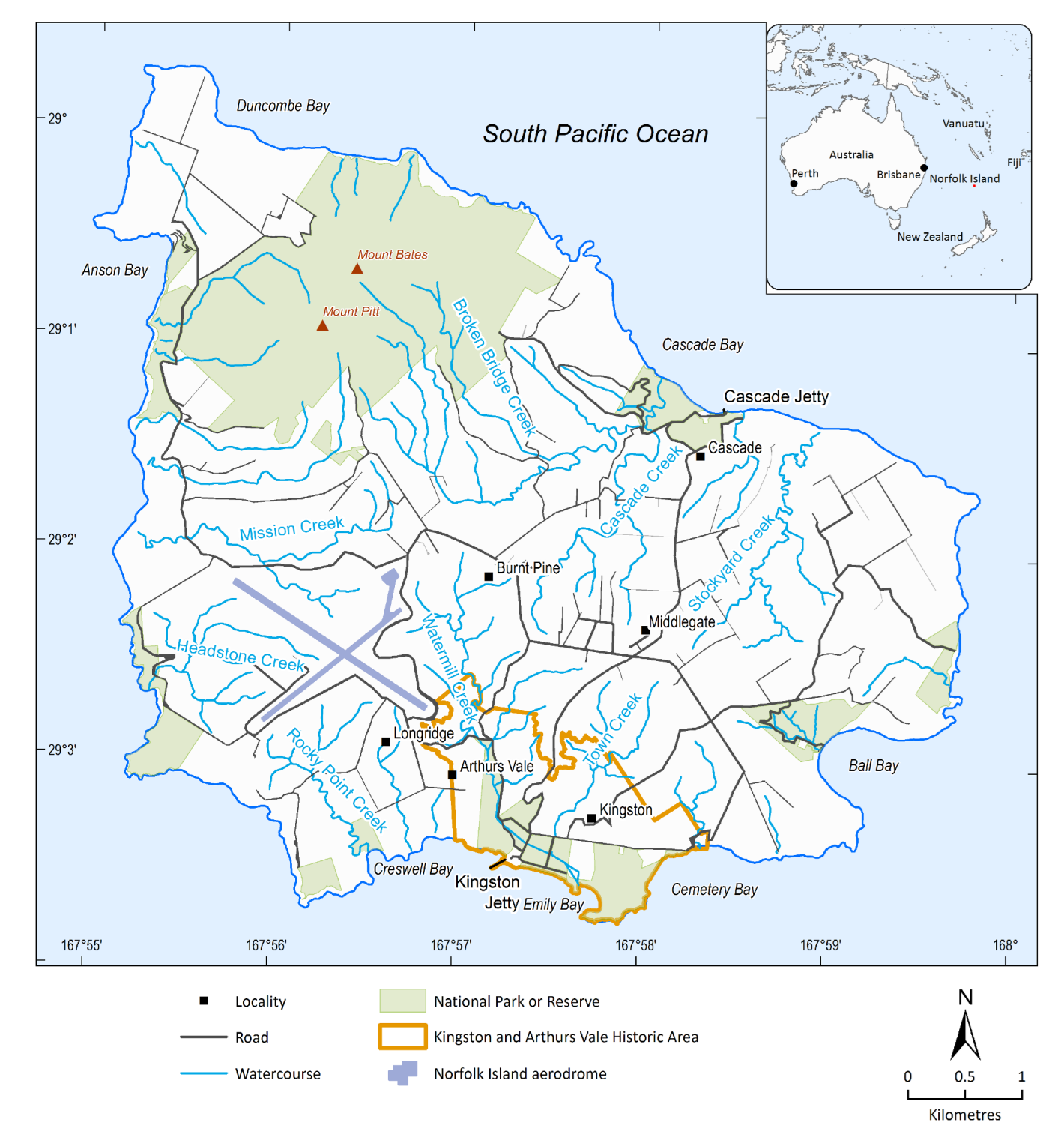
Norfolk island is situated in the south-west Pacific Ocean, occurring as small isolated island representing the only portion of the Norfolk Ridge protruding above sea level [8]. The island is 35.7 km in area (Figure 1). The Norfolk Ridge is a north–south trending submerged (except the very small island portions) continental ridge linking New Zealand and New Caledonia in the south-west Pacific Ocean. Norfolk island is a remnant of a weathered and eroded volcanic complex that began forming as a result of volcanic activity approximately two to three million years ago [9].
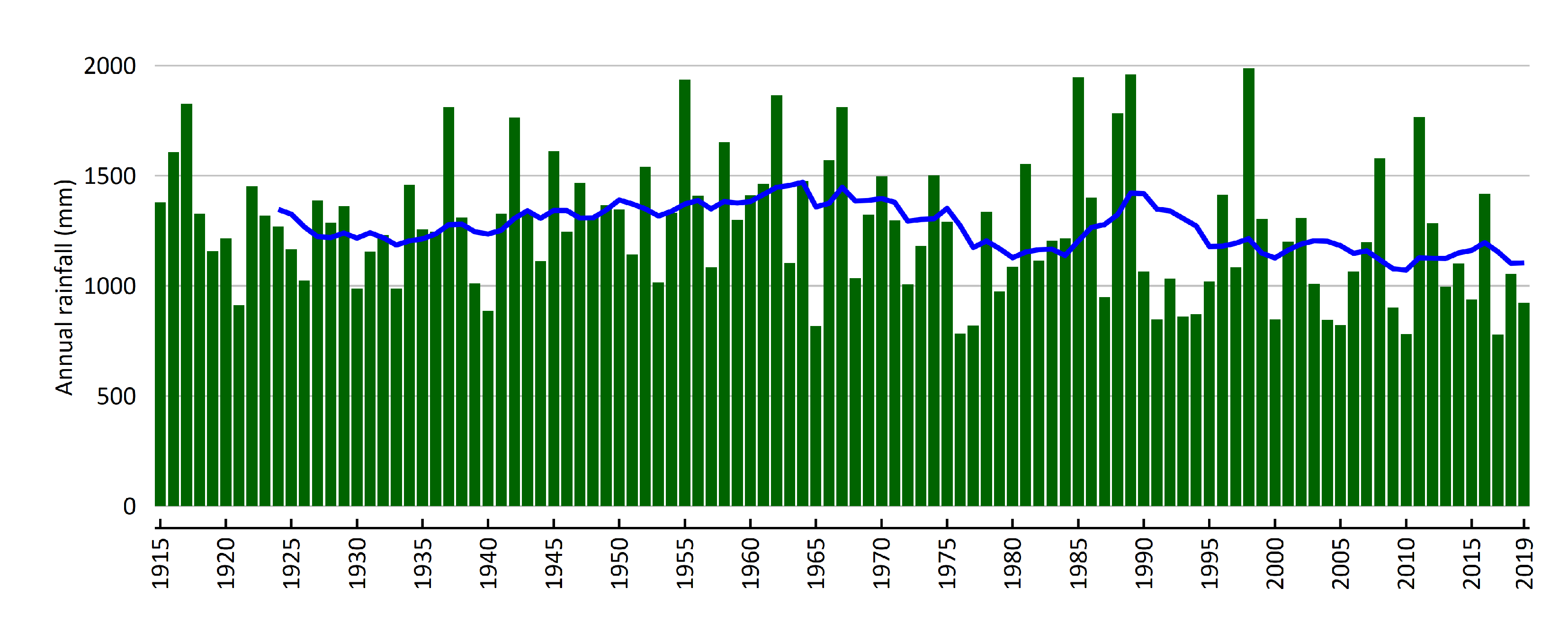
Norfolk Island had a mean annual rainfall of 1263 mm between 1915 and 2019. A notable feature in Figure 2 is the decline in annual rainfall since about 1970, which manifests as long runs of dry years in recent decades. Another feature of rainfall at Norfolk Island since about 1970 are the large fluctuations between exceptionally wet and dry years. These changes in rainfall are not anomalous to Norfolk Island but are part of a broad pattern of change, with south-eastern and south-western Australian also experiencing a decline in annual rainfall and change in seasonality of rainfall in recent decades.
Relative 1915 to 1969 (1334 mm/year) mean annual rainfall at Norfolk Island was 11% lower between 1970 and 2020 (1184 mm/year), and recent decades have seen mostly drier than average years, with annual rainfall during 33 of the last 50 years (66%) and 22 of the last 30 years (73%) having an annual rainfall less than the long term median (1915–2020). The decline has occurred in all seasons except summer, with the largest decreases in seasonal rainfall occurring during autumn and winter [10]. This is consistent with declines in autumn and winter rainfall observed over much of southern and eastern Australia. Rainfall over the three summer months typically accounts for about 20% of the annual total.
Characteristics of the condition of the soil surface affect runoff and water infiltration. All soils on Norfolk Island have firm strongly structured surfaces with rapid surface infiltration, and impeding subsurface layers are generally absent. Surface runoff only occurs during severe rainfall events when rainfall intensity is greater than surface infiltration rates or if soils are saturated (wet/shallow soils).
The soils and regolith derived from the basalts and tuff are deep (commonly as deep as 60 m) and the soils are quite permeable [6]. This, in combination with the humid climate and incised drainage lines, has resulted in strong surface water-groundwater connections across the island, as judged by the surface water and groundwater chemistry, and the once common expression of groundwater springs at the head of most drainage lines [6].
A strong surface water-groundwater connection, a high potential groundwater storage and a drying climate, lends the hydrology of the island to potential non–stationarity in hydrological prediction. Briefly, this is when the hydrological response of the catchment differs over longer time periods despite similar short-term climate inputs. This has been observed in the south-west of Western Australia where long-term drying has been experienced in a remarkably similar fashion (timing and severity) to Norfolk Island [11]. In that region, runoff coefficients have fallen dramatically, and even when wetter years are now experienced, runoff is far lower than from similar rainfall 40 years ago. These changes are largely the result of declining groundwater-surface water connection [12,13] and provide a challenge to the use of conceptual rainfall-runoff models [14].
Rainfall on Norfolk Island is, on average, higher in winter than summer, and combined with lower potential ET at this time, is the period when runoff is higher. The exception to this is storms in late summer/early autumn related to tropical depressions that can bring significant depths of rainfall in a short time period. Based upon this climate (Section 2), one may expect runoff coefficients in the range of 0.2 to 0.3 [15], which equates to mean annual runoff in the 250 to 375 mm range. However, the limited historical data on runoff indicates that runoff coefficient varies between 0.05 and 0.23 (Wheeler and Falkland, 1986). These data were collected at eight locations for the years 1981 to 1984. It should be noted that rainfall on Norfolk Island has, in general, been in decline since the mid-1970s.
At the last Australian Government census [16] in 2016 there were 1748 people on Norfolk Island and 1080 private dwellings of which 748 (75%) were occupied. Approximately 30,000 tourists visit the island annually, which assuming each stays an average of seven days is equivalent to an additional 575 permanent ‘visitors’. There is no reticulated water supply scheme on Norfolk Island, in part due to prohibitive cost of such a scheme given the dispersed nature of the residential population and the steeply undulating landscape. The majority of residents (>95%) primarily source their water from rainwater harvest/rainwater storage (RHRWS) and replenish their depleted rainwater tanks with groundwater sourced from a private bore/well, delivered by a commercial ‘water carter’ or from one of three communal water points on the island. Although there are 475 registered bores and wells on the island, no new bores or wells have been constructed since a moratorium on groundwater drilling was introduced in 1996.
3. Method
The water balance of a landscape in its most simple form can be expressed as;
where I is the input of water, O is the output of water and is the landscape change in water storage.
This can be further expanded into processes that can be measured or estimated as;
where P is precipitation, is evapo-transpiration, Q is runoff, is the change in aquifer water storage, is the change in soil water storage, while is groundwater discharge (including pumping from aquifers, transpiration by riparian vegetation and coastal/sub-marine discharge).
For this study the periods 1967–1976 and 2010–2019 were used to investigate the changes in water state, largely since data availability is highest during these periods and coincides with the data of Wheeler and Falkland [3], Abell [4] and modern data collected as a part of this study. A ten year period was judged to be long enough to reduce the effects of inter-annual variability. Individual components of the water balance (e.g., runoff) are presented in time periods suited to each individual analyses.
3.1. Potential Evapotranspiration and Irrigation Demand
Class A pan measurements are available on Norfolk Island since the 1970s and these may be indicative of evaporative demand. However, for longer term estimates of daily potential evapotranspiration (), estimates were made based on climate variables collected by the Bureau of Meterology at Norfolk Island Airport. These were, daily rainfall, maximum and minimum daily temperature, wind run, dew point temperature and cloud cover (both at 3-hourly intervals). These data were used to calculate Penman–Monteith potential evapotranspiration using the FAO56 method [17]. The Penman–Monteith equation, using specified units is as follows:
where is reference evapotranspiration (mm·day), is net radiation (MJ·m·day), G is soil heat flux (MJ·m·day), T is mean daily air temperature at 2 height (°C), is windspeed at 2 m (m·s), is saturation vapour pressure (kPa), is actual vapour pressure, is vapour pressure deficit (kPa), is the slope of the vapour pressure curve (kPa·°C−1) and is the psychometric constant (kPa·°C−1).
Of the above parameters, data were not available for soil heat flux, wind speed at 2 m, vapour pressure or radiation. For daily estimates the net soil heat flux G is assumed to be zero. For Norfolk Island, synoptic wind data at 10 m height was available as far back as the 1940s. These data were corrected to 2 m height using the relationships of Tennekes and Lumley [18]. Vapour pressure was estimated from relative humidity and temperature data. Incoming radiation was calculated from cloud fraction data, latitude and day of year information as follows (from Shuttleworth [19]):
where is the fraction of extra–terrestrial radiation () on overcast days, is the fraction of extra–terrestrial radiation () on clear days, is the cloudiness fraction, n is bright sunshine hours per day, N is total day length (hours) and is extra-terrestrial radiation (MJ·mday). The values of and were assumed to be 0.25 and 0.50 respectively [19]. was calculated using latitude, altitude and day of year.
The crop irrigation water demand estimates used the AWRA-R irrigation model [20], which is based upon the FAO56 [17] method of estimating crop water requirements. The model accounts for soil water availability and triggers irrigation events as the soil water becomes depleted by crop water use. Crop water use is calculated as follows:
where is the crop water requirement (mm·day), is the reference crop evapotranspiration (mm·day) and is the crop coefficient (dimensionless). Plant available water capacity was based on soil survey data and data regarding plant rooting depth from other locations.
3.2. Vegetation Mapping/History
Attribution of vegetation/land cover type across the study area was an important pre-cursor to recharge estimation, since vegetation type and structure will influence actual evapo–transpiration. Accordingly, high resolution airborne LiDAR was collected as a part of the study, providing both terrain and and vegetation morphology [21]. Similar approaches have been used to classify vegetation types including the extent of invasive weeds [22,23].
Prior to undertaking WAVES modelling of evaporation and potential recharge, the similarity in evaporation response for major vegetation types on Norfolk Island was examined using remote sensing. The remotely sensed method of inferring evaporation was based on the CSIRO MODIS ReScaled EvapoTranspiration CMRSET model [21]. The CMRSET model was developed to estimate AET using the MODIS nadir BRDF-adjusted reflectance (NBAR) product (called MOD43B4) available at a spatial resolution of 1 km × 1 km pixels. However, this spatial resolution is not fine enough for differentiating the different landcover types on Norfolk Island, so the less temporarily frequent Landsat data series was used instead (at a pixel size of 30 m × 30 m). The remotely sensed mean AET values were compared at a selection of points across the island covering: Eucalypts (6 points), Norfolk Pines (12 points), Pasture (12 points), deep rooted woody weeds African Olive (17 points) and Red Guava (17 points). The results indicated that Eucalypts have high AET values and are very similar to the woody weeds (African Olive and Red Guava). Norfolk pines and pasture tend to have lower AET values. With no WAVES vegetation parameters readily available for woody weeds, woody weeds were modelled using the eucalypt WAVES parameters, given their similarity in remotely evaporation response.
In this study, LiDAR was combined with spaceborne remote sensing products (e.g., high resolution RGB imagery and ALOS-2 synthetic aperture radar intesity). These data were calibrated to local expert data regarding vegetation types and extent. A machine learning classification model was used to predict vegetation types and extent and these were tested against an independent set of validation data not used in the model training. The machine learning algorithm was the random forest classifier Pal [24], Belbiu and Drăgut [25], and was trained across 128 decision trees to produce three levels of classification (Table 1).
Historic estimates of land cover were reconstructed from historical records and aerial photography.
3.3. Groundwater Monitoring
In 1996, a moratorium on the construction or alteration of bores and wells was introduced at which time there was approximately a total of 500 groundwater bores and hand-dug wells across the island [4,26]. However, it should be noted that long-term residents on Norfolk Island also speak of many abandoned holes and ‘unregistered’ bores.
As part of this study, a hydrological monitoring programme was initiated to better characterise and conceptualise the groundwater systems as well as quantify their groundwater balance. Local residents, business owners and island Administration provided permission to access and monitor groundwater levels at 65 locations from 42 bores and 23 wells. Periodic manual static groundwater level observations were recorded at all 65 sites where a standing water level could be obtained with a portable hand-operated electronic water level meter. Temporal groundwater level observations were obtained over an 11-month period from the installation of digital temperature and pressure data loggers at 20 sites. In addition to observations recorded in groundwater bores and hand-dug wells, observations of the most elevated point of perennial groundwater seepage to creeks was recorded at 12 locations and used as proxy for the watertable. All groundwater level observations collected were reduced to the Australian Height Datum (AHD) and used as input to produce hydrographs as well as modelled ‘modern’ (2019) and ‘historic’ (1975) potentiometric surfaces across the island.
3.4. Geological Modelling
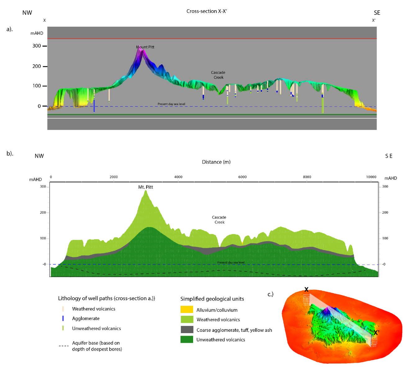
A three-dimensional geological model of Norfolk Island was developed to improve the understanding of the subsurface geology and hydrogeology, and to assist with the water resource assessment. Prior to development of the three-dimensional geological model, lithological logs, which generally only existed as hard copies, were digitised and extensive data quality checks were performed. The lithological logs were then interrogated in three-dimensional space, subjected to further data quality checks and simplified to reduce the number of lithological classes for representation in the three-dimensional geological model. This initial study confirmed that multiple sequences of basalt flows and other volcanic lithologies (e.g., ash, tuff and agglomerates) exist within the subsurface. However, the variable and often high degree of weathering particularly in the upper part of the subsurface (with rocks ranging from slightly weathered to completely decomposed) prohibited correlations of individual basalt flows, and the weathered shallow volcanic sequences were therefore summarised into a single geological model unit (weathered volcanics). The median thickness of the weathered volcanic sequence is 43 m. Beneath this weathered sequence, deep coarse agglomerates, unweathered basalts (in drillers’ logs sometimes described as fractured or dense) and hyaloclastites were identified in lithological logs. Comments in drillers’ logs highlighted that the primary water source in many bores appears to be basal coarse agglomerates, followed by fractured and unweathered basalts and weathered basalts. Despite their hydrogeological significance, the basal coarse agglomerates, fractured and unweathered basalts and hyaloclastites were summarised in the three-dimensional geological model unit as a single unit (unweathered volcanics), as a further assessment would be needed to confirm their spatial continuity. Additional lithological units included in the three-dimensional geological model are alluvium and calcarenite.
The ground surface (topographic) elevation and sea floor elevation used for the three-dimensional geological model development is based on the newly obtained LiDAR survey for Norfolk Island and an historical bathymetry dataset, covering an area to a distance of 300 m offshore. A variable offset between with a mean of 2.45 m was observed between LiDAR and bathymetry and the bathymetry was therefore raised by 2.45 m. These two datasets have been blended to derive a combined dataset with a 5 m spacing. This combined dataset was imported into GoCAD three-dimensional geological modelling software, where it was used to determine the elevation at each bore location.
The three-dimensional geological model was then used to assign bores to different aquifers and estimate changes in saturated and unsaturated aquifer volumes based on an historical potentiometric surface from 1974 to 1975 [4] and the modern (2019) potentiometric surface, as well as the change in saturated and unsaturated cliff areas.
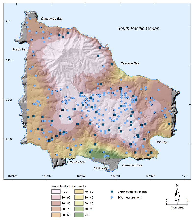
3.5. Potentiometric Surface
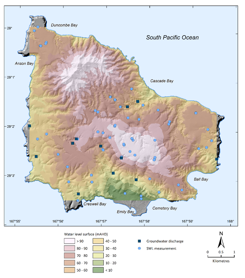
Historic potentiometric surface were estimated using 203 groundwater level observations (58 groundwater bores and 145 groundwater wells) and 56 inland seepages as defined and mapped by Abell [4]. The seepage sites were digitised from the data published in Abell and Falkland [6]. Reduced standing water levels (RSWL) for each groundwater level measurement location (i.e., bores and wells) were derived by subtracting observations from either the surveyed elevation at the measurement location, or the natural surface elevation defined by a digital elevation model (DEM) derived from the LiDAR survey. Similarly, modern (2019) potentiometric surfaces were estimated using 65 groundwater level observations (42 groundwater bores and 23 groundwater wells) compiled between May 2019 to May 2020 and surface groundwater discharge observations derived by walking along drainage lines in a period where significant rain had not been observed for weeks and noting the presence or absence of surface water flow (analogous to the “seeps” of Abell [4]).
A simple cokriging interpolation method was developed using the Abell [4] RSWL values and seppage locations as an input. The LiDAR data was re–sampled to derive a 5 m DEM which was used as the covariate input variable. The resulting potentiometric surface was assessed against known documented historical observations.The same cokriging method parameters were used to interpolate a modern potentiometric surface using the study RSWL values and seepage observations as input. The resulting surfaces were then classified into ranges of water level elevation.
3.6. Groundwater Recharge
Due to the challenges in estimating recharge, this study used several independent approaches to derive recharge rates across Norfolk Island. Two methods were used to estimate recharge (i) generic relationships [27], and (ii) soil-vegetation-atmosphere transfer modelling (WAVES) [28].The only method for which it was possible to estimate seasonal or annual recharge was using the WAVES model, which estimates deep drainage or potential recharge. Generic relationships being derived from long-term average datasets only provide estimates over similar timeframes. In this way it is not suited to estimating recharge under transient processes such as climate or land use change. Key input data required by WAVES are climate data, which were obtained from the Norfolk Island airport and soil and vegetation parameters.
Based on the experience and advice of the CSIRO soil officers the most similar Ferrosols in Australia to Norfolk Island are found in the Burnett region, Queensland. A soil physics study on the Ferrosols in the Burnett characterised the soils as having large drainable porosities in all parts of the profile to a measured depth of 1.5 m, with very rapid rates of internal drainage [29]. This is consistent with field observations on Norfolk Island. During the short field program undertaken as part of this study two rainfall events of between 40 and 50 mm·day were recorded, neither of which generated runoff in any of the small catchments being monitored.
The Broadbridge and White soil physical parameters used for the WAVES modelling on Norfolk Island are listed in Appendix A Table A2. Soil parameters for the first two soil layers were taken directly from Bell et al. [29]. The third soil layer, below 1.8 m and below the depth of measurements made by Bell et al. [29], was based on expert judgement. The weathered rock is known to texture to a sandy loam with hard lumps, however, the weathered rock is permeable, though it is not considered to be as permeable as the soil. Typical soil parameters for a sandy loam were adopted from Dawes et al. [30].
The main woody weed species are African olive (Olea europaea), red guava (Psidium cattleianum), cottoneaster (Cotoneaster frigidus) and Hawaiian holly (Schinus terebinthifolius) and the major pasture species are warm season perennial grasses, namely kikuyu (Pennisetum clandestinum), Rhodes grass (Chloris gayana), paspalum (Paspalum dilatatum) and clovers (Trifolium spp.) [31]. Due to the absence of WAVES vegetation files for many of the above listed species, WAVES modelling was limited to three vegetation types, for which data were available and were deemed likely to be suitable surrogates for modelling deep-rooted and shallow-rooted vegetation on Norfolk Island. The three vegetation types were:
- 1.
- Eucalypts
- 2.
- Maritime pine (Pinus pinaster) (used as a surrogate for the Norfolk Island Pine)
- 3.
- Generic C4 perennial pasture.
3.7. Streamflow Measurement and Estimation
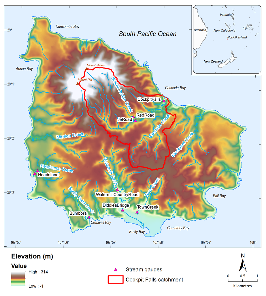
There have been several previous attempts at measuring streamflow on Norfolk Island. Of these, only the Wheeler and Falkland [3] study records any observed streamflow data, and, in all known studies, hydrological observations have ceased at the close of each project. Despite previous projects in which runoff was gauged, monitoring of surface water hydrology has been intermittent on Norfolk Island. Furthermore, most data collected during these studies cannot be located at the time of writing. The only recoverable data were from tables within the Wheeler and Falkland [3] report. This report contains approximately 3 years of daily flow at the Cockpit Falls (Cascade-Figure 3). Various other sites at Town Creek, Stockyard Creek, Rocky Point Creek, Mission Creek, Headstone and Watermill Creeks were reported at a monthly scale across the same time period (April 1981 to June 1984). These additional sites relied upon daily staff gauge readings. Some of these sites featured thin-plate v-notch or Cippoletti weirs, although confusingly, many of the same sites were recorded as having a ‘rock-bar’ control. The authors state in the conclusions that there were many problems with the data. As a part of this study, pressure sensors and loggers were installed at a number of sites between May and October 2019, and these sites continue to be monitored. No attempt was made to calibrate a rainfall-runoff model in any locations other than Cockpit Falls, since it was the only catchment with daily historical data available.
3.8. Conceptual Rainfall–Runoff Model Calibration
Two conceptual rainfall-runoff models were tested for their performance, Sacramento [32] and GR7J [14]. The models were calibrated to the observed data and tested against an objective function that considered simulation bias, low flow and high flow fit as well as overall correlation. The objective function is as follows:
where is the Nash–Sutcliffe Efficiency of root transformed daily flow, is normalised error for 100 day segments, is normalised error for the 10 highest flow days, is simulation bias and;
where is the exceedance probability difference of the 80%ile, non-zero exceedance value of the observed data in comparison to the simulated data and is the probability of 80% exceedance value calculated from concurrent simulated and observed time series. This objective function was favoured since it has been shown to produce a more balanced simulation that considers fit across the flow duration curve and at daily and annual time scales [33].
Estimates of runoff and streamflow were required at multiple locations without streamflow observations (ungauged areas). The approach undertaken in this study was to transpose the model parameters from Cockpit Falls to other parts of the island. However, the model parameters calibrated at Cockpit Falls gauge are representative of a catchment with a connected groundwater system in its lower reaches (i.e., groundwater discharge is occurring in the lower reaches). Hence the appropriateness of applying these model parameters to other parts of the island depended upon the similarity of groundwater characteristics and areas of saturation following large rainfall events in these other catchments. In many (more elevated) parts of Norfolk Island the current potentiometric surface was a considerable distance (i.e., >10 m) below the ground surface and consequently streamflow estimated from the application of the model parameters calibrated at Cockpit Falls was inappropriate as there would be very little or no baseflow in those areas. To produce estimates, the simulation at Cockpit Falls was modified in two steps:
- 1.
- A digital baseflow filter [34] was applied with a low alpha value ( = 0.001), and this was subtracted from the Cockpit Falls simulation to provide an intermediate estimate, which was further modified by:
- 2.
- Applying a high pass filter of the following design:
where is the intermeadiate flow estimate (after baseflow separation).
Is it worth nothing that we recognise that this quick flow is still likely to be an overestimate as some of the quickflow is likely to be generated in areas with shallow water–tables. Nonetheless, even though this is likely to be an overestimate the value is still very small (probably within measurement and modelling error) and hence still serves its purpose in this study.
3.9. Groundwater Discharge
3.9.1. Transpiration of Groundwater by Vegetation
Groundwater within the root zone of some terrestrial vegetation can be used by the vegetation as a source of water [35,36], in small catchments (i.e., <40 km) this can manifest itself as diurnal changes in streamflow under baseflow conditions as vegetation transpires water during the day and not the night. To calculate the transpiration of groundwater by vegetation pressure loggers were installed in selected perennial streams across the island and the method outlined by Boronina et al. [37] was used to diurnal signals in stream water level to a transpiration flux. Although diurnal fluctuations can also be induced by a variety of factors such as alternating processes of freezing and thawing, early afternoon rainfall events in the tropics, changes in streambed hydraulic conductivity induced by temperature variations, hydro-electric power generation, and time varying rates of groundwater extraction [38], on Norfolk Island the most likely explanation is considered to be the diurnal cycle of water uptake by vegetation (primarily due to diurnal changes in solar radiation and air temperature), where streamflow is highest at dawn and lowest in the afternoon.
3.9.2. Coastal Spring, Submarine and Diffuse Cliff Discharge
At the scale of an island-wide water balance, ‘aquifer discharge’ is considered to be the discharge of groundwater through the saturated profile of the cliffs that surround much of the island, and groundwater that discharges directly into the ocean, commonly referred to as submarine groundwater discharge (SGD). Both processes are difficult to quantify, and no measurements or estimates exist for Norfolk Island. Due to the time frames of this study and available resources and challenges in undertaking these measurements, no direct measures of SGD or coastal seepage were made and aquifer discharge is inferred here as the residual term in the water balance.
3.10. Consumptive Water Use
Total anthropogenic groundwater use over time was estimated for the following categories using the methods summarised below;
- 1.
- Residential households-based water use survey and RHRWS shortfall calculations by Seo [39].
- 2.
- Commercial agriculture-high-resolution aerial photography to identify total area, local knowledge was used to define cropping practices and FAO56 crop modelling to calculate water use per hectare.
- 3.
- Medium and large-scale vegetable gardens and orchards-high-resolution aerial photography to identify total area, local knowledge was used to estimate percentage of gardens likely to be irrigated (in which case they would be irrigated using groundwater) and FAO56 crop modelling.
- 4.
- 5.
- Tourists-to understand the potential water use of tourists to Norfolk Island, loggers were installed in rainwater tanks of two tourist accommodation businesses and average water use numbers were extrapolated based on tourist visit records held by the NIRC.
- 6.
- Other industry and services-Other industry and services include school, hospital, construction and council operations. No information was available on groundwater use by other industries but local knowledge indicated that it is small compared to other consumptive use categories and consequently a nominal value was assigned.
4. Results
4.1. Climate
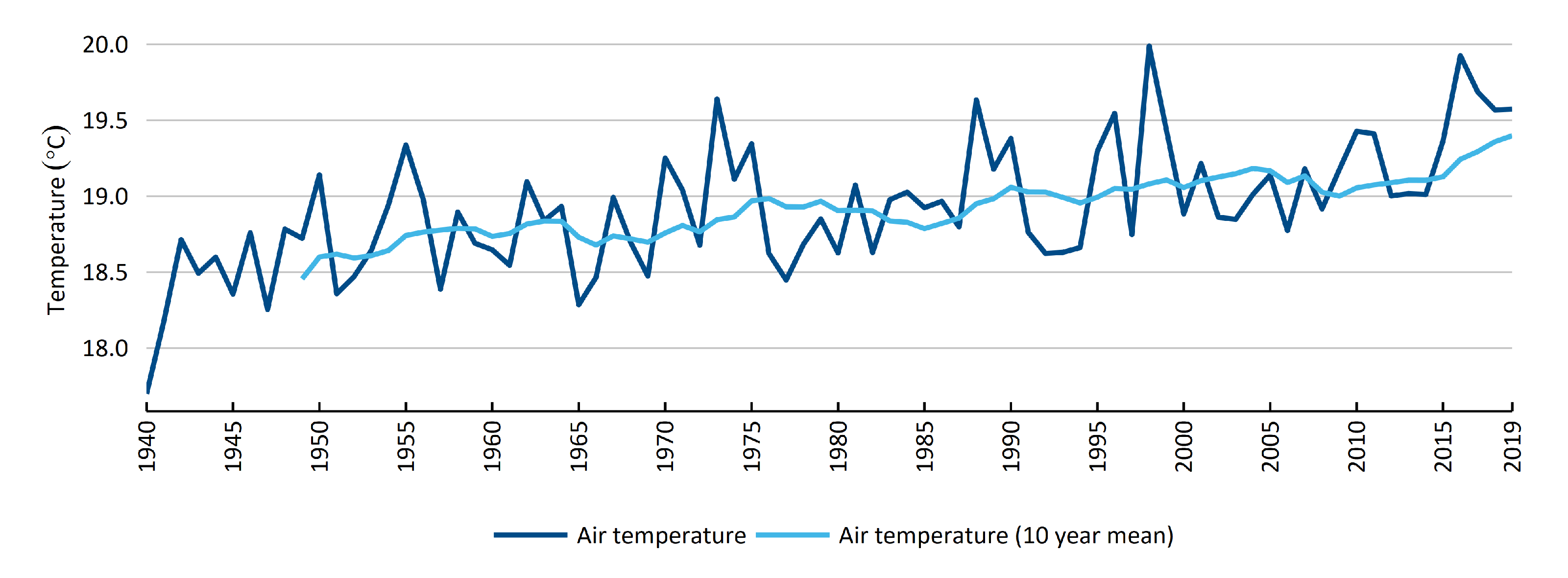
While decreases in long-term rainfall on Norfolk Island have been previously documented [40], changes in pan evaporation and potential evaporation have not been previously reported. There has been an increase in mean annual air temperature over Norfolk Island (Figure 4), and while mean air temperatures have increased in each of the four seasons, spring months have recorded the greatest increase (0.085 °C/decade). BoM (2020) report a similar increasing trend in sea surface temperature.
There is a weaker correlation between pan evaporation and mean temperature, but both show increasing trends, with a 14% increase in pan evaporation for each degree of warming, relative to the mean pan evaporation between 1981 and 2010. Increases in pan evaporation at Norfolk Island (Figure 5) are also likely to be due to an increase in wind speed over Norfolk Island since about 1990, which is consistent with other studies that have found surface wind speed to have increased over the ocean [41] but decreased over land [42] the past three decades.
Reference crop evapotranspiration based on the FAO56 method [17], shows a considerable increasing trend in crop/plant water demand, in part due to an increase in temperature, but more notably from the increase in wind speed from about 1990 [43]. The increasing trend in crop/plant water demand combined with the decreasing trend in rainfall, results in a strong upward trend in modelled irrigation water requirement.
4.2. Potentiometric Surfaces
The modern potentiometric surface (2019-Figure 6), while more data sparse shown than historic surfaces (1975-Figure 7) exhibits similar spatial patterns to the historical surface. Areas on the southern part of the island plateau still exhibit groundwater levels of 100 mAHD in places based on measurements between May 2019 and March 2020. The 65 SWL measurements used as input to derive the potentiometric surface come from a combination of groundwater bores and wells intersecting the watertable in the weathered volcanics, as well as areas where the watertable is in shallow agglomerate and unweathered (fractured) basalt. The highest areas of uncertainty remain the same as for the historical surface (beneath Mount Pitt and Mount Bates along the western side of the island between Mission Creek and Anson Bay).
The historical potentiometric surface exhibits much larger areas of the southern plateau with higher groundwater levels, though it is underpinned by a much larger spatial dataset. In addition, hydraulic gradients are also more subtle towards the eastern and western discharge areas for aquifers in the weathered volcanics. It is important however to acknowledge that the surfaces were derived from static observations that are likely to be spatially affected by frequent groundwater pumping at some locations and less so at others.
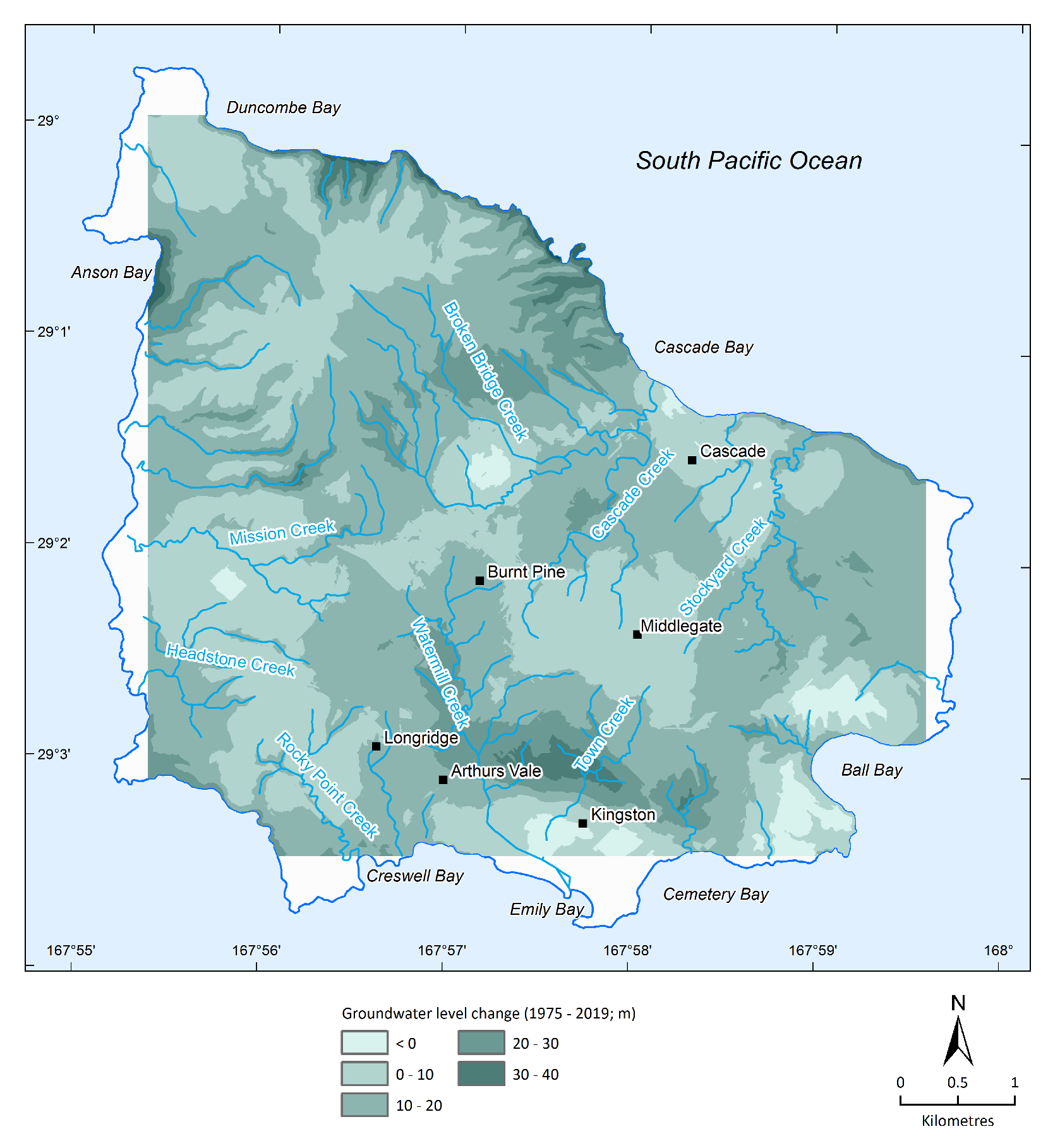
The modelled change in groundwater levels was derived by calculating the difference between the historical (1975) and modern (2019) potentiometric surfaces. Figure 8 shows the spatial differences in modelled changes to groundwater levels over the last 45 years. Groundwater levels have declined between about 5 and 20 m across different parts of the island. The largest decline in groundwater levels appear to be between the upper reaches of Town Creek and an area adjacent to Ball Bay. Areas of little change reflect the lack of groundwater level observations in both potentiometric surfaces across these areas.
4.3. Geological Modelling
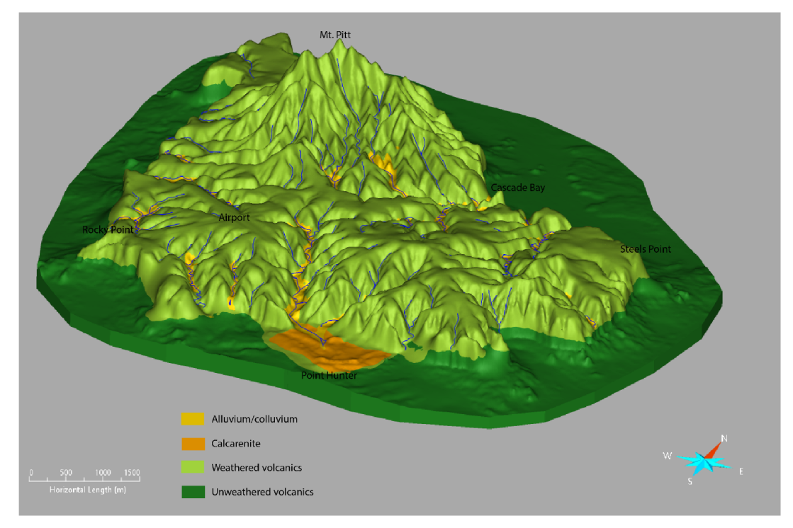
From the initial assessment of lithology and water-bearing formation, a smaller number of relevant lithological classes were identified for inclusion into the three-dimensional geological model. These were alluvium, calcarenite, weathered volcanics, bassal coarse agglomerate and yellow ash, unweathered (fractured)basalt and hyaloclasite.
Due to the relatively small number of deeper bores and as it is considered likely that the basal coarse agglomerates, unweathered (fractured) basalts and hyaloclastite are hydraulically connected, it was not considered necessary for the first model iteration to include them into the three-dimensional geological model as separate model units, and they were therefore combined into a composite model unit named ‘unweathered volcanics’. Above this unit, multiple repetitive sequences of volcanic lithologies (e.g., basalt, agglomerates, ash or tuff) can be identified within the upper approximately 50 m of the subsurface in the lithological dataset. In contrast to the deeper unweathered volcanics, these shallower volcanics are typically highly weathered and sometimes decomposed. The spatial variability of the degree of weathering is highly variable. This means that although they can be identified and separated clearly in some bores, elsewhere they are highly weathered or decomposed. They are therefore combined into a single three-dimensional geological model unit (‘weathered volcanics’). Furthermore, alluvium and calcarenite (limited to the coastal area at Jetty Bay) were included as separate model units in the three-dimensional geological model.
The completed four-layer three-dimensional geological model of Norfolk Island is shown in three dimensions in Figure 9 and as cross-sections in Figure 10. The deep basal agglomerates and yellow ash form a characteristic bed at the top of the unweathered volcanics, and they form a major water source of bores on Norfolk Island. The depth at which the unweathered volcanics were intersected varies, but the median thickness of the weathered volcanics overlying the unweathered volcanics is 43 m. However, in some areas, and in particular underneath Mount Pitt where no bores exist, the interface between weathered and unweathered volcanics remains uncertain.
Following the completion of the three-dimensional geological model, additional models were developed to compare how the saturated and unsaturated rock volumes change from 1975 (based on the dataset from Abell (1976)) to 2019 (based on the modern potentiometric surface). For the purpose of this study, it was initially assumed that the base of the aquifer is the modern-day sea level. However, as shown on cross–sections through Norfolk Island (Figure 10), multiple groundwater bores extend beyond the depth of the modern-day sea level. Therefore, an additional set of models was developed where the base of the aquifer was represented by a surface interpolated from the deepest bores developed on Norfolk Island. The study showed that there has been a significant decline in the potentiometric surface from 1975 and 2019 (Table 2). When assuming the sea level as the aquifer base, the saturated rock volume (as total rock volume rather than water volume within the rocks) decreases by about 15% from 1974 to 1975 and 2019, compared to a decrease of approximately 12% when assuming the surface developed from the deepest bores as aquifer base. This significant change is also reflected in the change of the exposed cliff surface area that is unsaturated or saturated, respectively. In 1974 to 1975, approximately 24% of the cliff surface exposure area was unsaturated, whereas in 2019, the estimated unsaturated cliff surface exposure area has almost doubled to 46%.
Modelling based on available data, and assuming a porosity of 0.1, indicates that the volume of rock saturated by water has decreased by about 45,000 ML (±50%) or about one-fifth of the stored volume since the mid-1970s. Three-dimensional geological modelling indicates that of 500 known wells and bores, the number of ‘dry’ wells and bores increased from about 70 to 210 in late 2019. If groundwater levels fell uniformly by a further 10 m and 20 m across the island, the number of dry wells would increase to about 325 and 400 respectively.
4.4. Groundwater Recharge
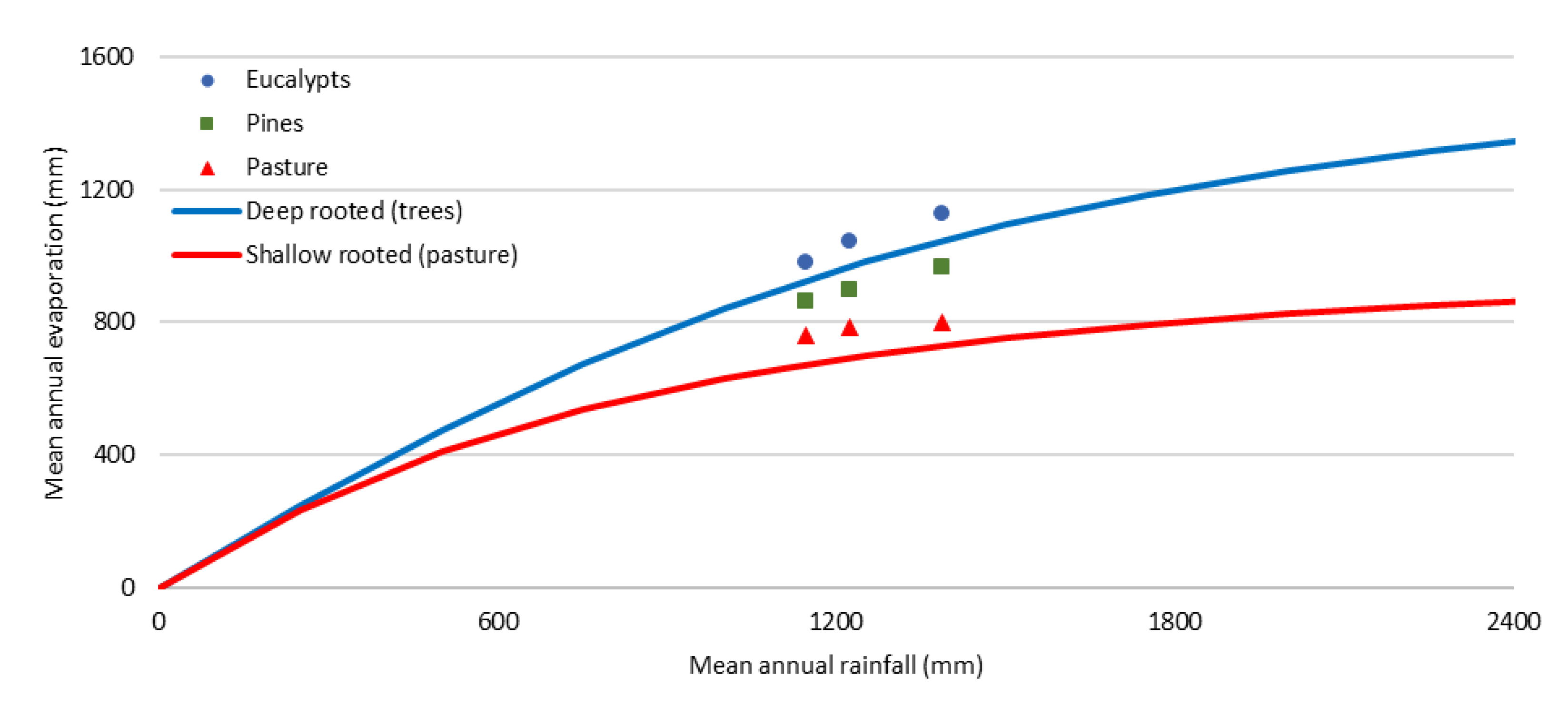
For comparative purposes the WAVES data were averaged over 25-year windows, which is a time frame commensurate with that of the data underpinning the relationships. These data were compared to theoretical relationships between rainfall and actual evaporation taken from method of Zhang et al. [27]). See Figure 11. The WAVES modelled actual evaporation under eucalypts, was slightly higher than that modelled under pines, which were higher again than that under pasture, while a declining trend in actual evaporation is evident for all vegetation types across the simulation period. Between 1945 to 1969, 1970 to 1994 and 1995 to 2019 mean annual rainfall reduced by 12% and 17% respectively relative to mean annual rainfall from 1945 to 1969. However, modelled potential annual recharge relative to the 1945–1969 period fell under eucalypts fell by 27% and 35% respectively (Table 3).
4.5. Streamflow Estimation
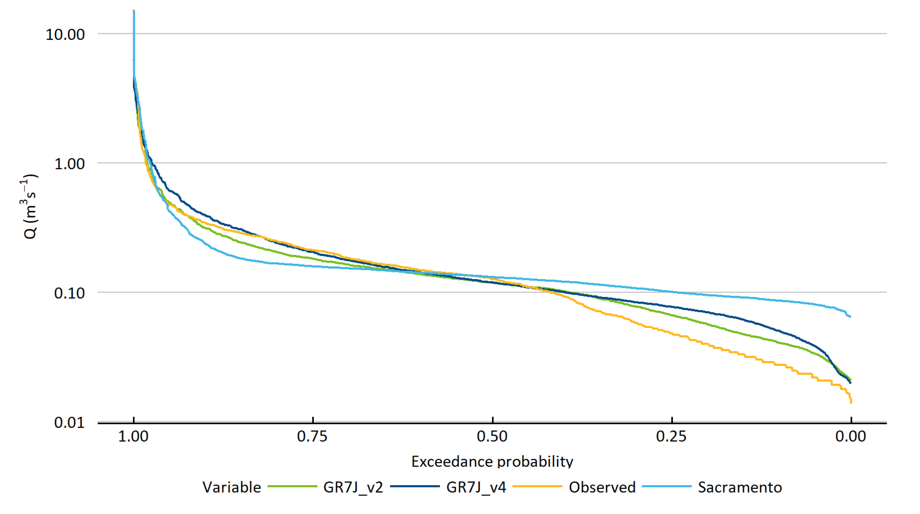
Simulated streamflow time series for the Cockpit Falls catchment was compared to streamflow observations at this site. Two versions of the GR7J model and one of Sacramento were evaluated. The goodness of fit was judged to be poor for all models deemed plausible, and all models underestimated flow in the 2019–2020 period (Table 4).
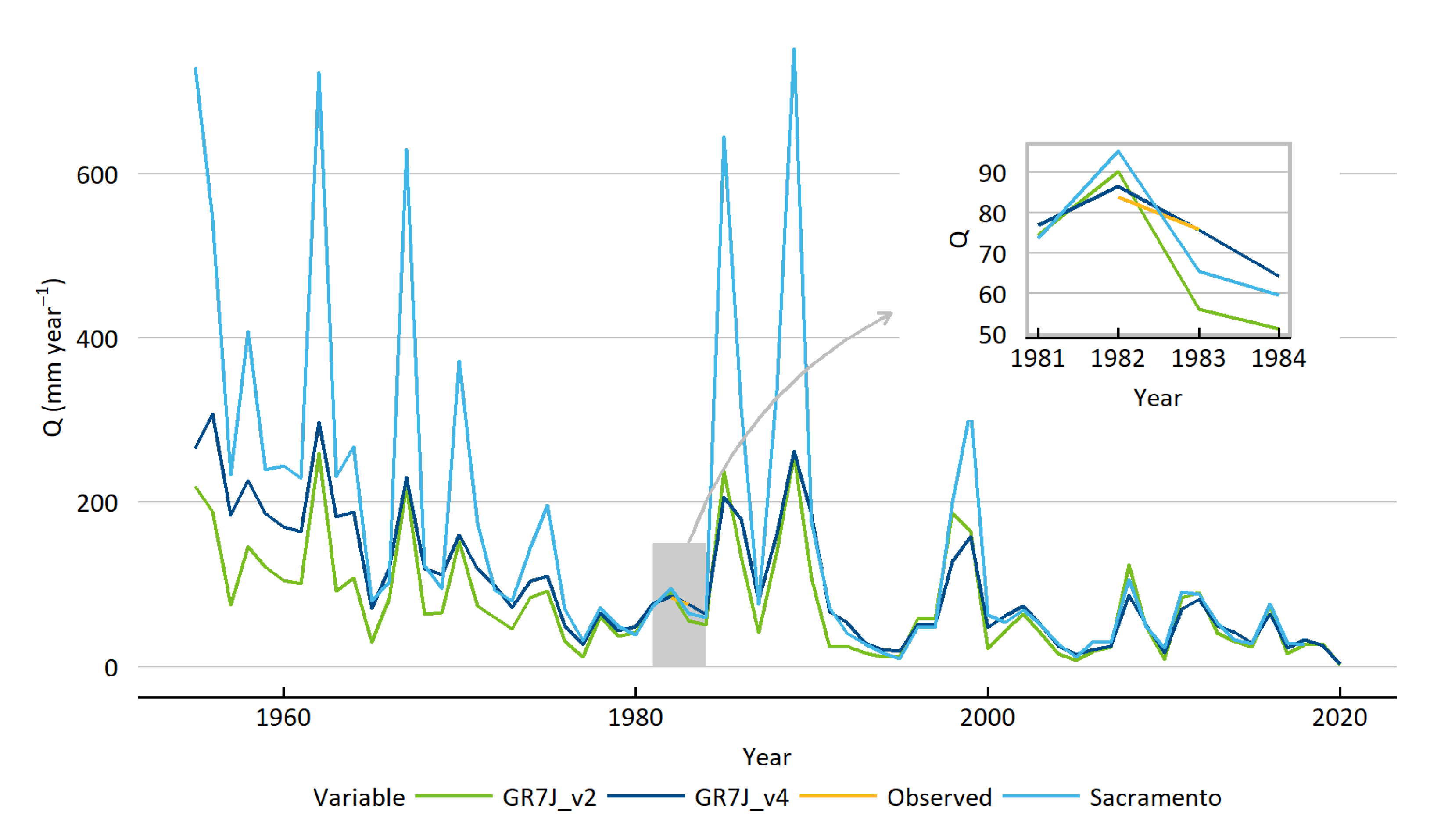
Consideration of these statistics along with flow distribution (Figure 12) as well as longer term model behaviour outside of the calibration periods was considered. The difficulty of simulating a suitable runoff time series is illustrated in Figure 13. All three simulations are similar in terms of performance against observed data, however the period of observation is very short relative to the simulation period (1950 to 2019). This is further compounded by a significant reduction in rainfall across the simulation period (Figure 2). While all models are similar in the observation period, they are vastly different during the 1960 to 1980s. It is very difficult to know which model represents true runoff from this time. The Abell and Falkland [6] report indicates that springs/seepages were evident at the head of most flow lines in 1974, suggesting a widespread groundwater–surface water connection at the time, and, potentially runoff coefficient was very high at that time. The runoff coefficient was for all models varied from approximately 4% to 20% depending upon model and decade of calculation, although most model/decade combinations were less than 10%.
A GR7J model was also calibrated for the Town Creek catchment, although there was little data with which to constrain the model. The calibration utilised a regression relationship between Cockpit Falls and Town Creek gauges published by Wheeler and Falkland [3], to estimate Town Creek streamflow.
Wheeler and Falkland (1986) also noted that the rainfall–runoff coefficient was low at Cockpit Falls at around 6%, while rainfall–runoff coefficients over a concurrent period of time at Town Creek, Watermill Creek and Rocky Point (named Bumboras in this study) were higher at 23%, 12% and 14% respectively. These differences were attributed to catchment losses due to groundwater movement out of the Cockpit Falls catchment. Since gauges for the other catchments were closer to sea level, losses were supposed to be lower. The Cockpit Falls catchment terminates in, as the name suggests, a waterfall. The gauge is 40 m above sea level, and it is possible that significant volumes of water are discharged from the catchment subsurface. However, this cannot be confirmed with data available at the time of writing.
Water balance estimates were produced using model outputs for the Cockpit Falls and the Town Creek site to provide some contrast between a ‘dry’ and a ‘wet’ site. Town Creek has a far higher runoff coefficient relative to Cockpit Falls and hence ET + losses at Town Creek are lower than potential ET. This is not the case for Cockpit Falls, and this is related to the very low runoff coefficient at this site, making extrapolation of these data across the Island difficult. It should be noted that the Town Creek catchment is south facing and more incised than the Cockpit Falls catchment, therefore, radiation at the ground surface and resulting energy for ET may be lower than calculated above. Additionally, it is very likely that the groundwater contributing area for Town Creek extends beyond the surface water catchment.
Of the three candidate models, GR7J-v2 was chosen as the parameter set for future climate runoff estimation since it was judged to provide a more conservative estimate of runoff over all conditions. The water balance components for both Cockpit Falls and Town Creek catchments is shown in Table 5. In groundwater disconnected areas using flow transformation as described above, the runoff coefficient reduces from 6.4% to 0.9% for the period 1950 to 2019. However, it should be noted that the resulting runoff time series may still be a slight over–representation of runoff in disconnected areas as the influence of groundwater induced areas of saturation on overland flow may still be implied in the original runoff time series.
4.6. Consumptive Groundwater Use
Estimates of anthropogenic groundwater use are shown in Table 6.
4.7. Waterbalance
A water balance for the entire island is provided in Table 7 based on estimates for different parameters discussed earlier in this chapter. The estimate of discharge from coastal seepages/SGD and cliff line vegetation is the residual of the difference between potential annual groundwater recharge and the sum of anthropogenic use, discharge to creeks and transpiration by vegetation in creeks. The modelled difference in volume of water stored in the island aquifers between 1975 and 2019 is 45,000 mL, which over a period of 45 years is an average reduction of 1000 mL/year (with a likely uncertainty of ±50% based on a likely range of averaged effective porosity values).
Calculated from the geological model of Norfolk Island, the exposed area of cliff line below the historical (1975) potentiometric surface reduced from 3.4 km to 2.41 km below the modern (2019) potentiometric surface. Although coastal seepage is localised, dividing the coastal seepage/SDG/cliff vegetation term in Table 3, Table 4, Table 5 and Table 6 by the exposed ‘saturated’ cliff surface in 1975 and 2019 gives an average groundwater flow velocity of 2.25 and 2.7 m/year. If coastal discharge (seeps and vegetation) was limited to 10% of the ‘saturated’ exposed face of the cliffs surrounding Norfolk Island then these averaged flow velocities would increase by a factor of ten, still within a plausible range. This assumes no SGD. Making an allowance for SGD would reduce these values.
5. Discussion
A water balance approach is a common method used by hydrologists to understand the properties and idiosyncrasies of study areas. Ideally, this would be facilitated by long-term data across multiple water balance components. In the case of small islands, a lack of infrastructure and trained staff means these data are rarely available. Physically, small islands have additional challenges for hydrologists, specifically sub-marine discharge, groundwater-sea water interactions and multiple small watersheds [2].
Norfolk Island, at 35.7 km is typical in both size and available hydrological data. Some data are available from investigations in the 1970’s and 1980’s, while poor archiving means that data from some subsequent investigations cannot be recovered. Norfolk Island is also typical of small islands in that it’s water supply to the population is vulnerable to changes in climate. This has recently become apparent as rainfall has declined, placing stress on the supply of water that in general, consists of water tanks supplemented by groundwater pumping. This study was intended to collect and analyse additional data, allowing a more informed understanding of the water balance of the island and changes to the water balance over the past 40–50 years.
For the period 1970 to 2020, the mean annual rainfall on Norfolk Island was 11% lower (at 1184 mm/year) relative to the 1915 to 1969 period (1334 mm/year). Rainfall decline has occurred in all seasons except summer, with the largest decreases in autumn and winter. These observations are consistent with broader patterns of climate change in the south–western Pacific [40].
Long-term changes in rainfall have resulted in a profound change to the hydrology of Norfolk Island. Water balance calculations indicate that the percentage reductions in long-term groundwater recharge and streamflow to be 2.1 and 4.3 times the percentage reductions in long-term rainfall over the same time period respectively. While rainfall has reduced by 13% across the study time period, evapo-transpiration has decreased by only 8%. This may be partly influenced by the decrease in pasture area over the time period (Table 8), with a concurrent increase in the area of woody weeds or deep rooted vegetation and an increase in reference crop evapotranspiration (Figure 5).
Across the study time period there has been 50% increase in anthropogenic use of water resources. However, even in the 2010–2019 period this was still less than 2% of estimated recharge and is therefore a very small component of the water balance. Despite this, there have been large reductions in groundwater heads in some parts of the island (Figure 8), that have created problems for water users. These result from an imbalance between groundwater discharge and recharge that will need to be considered for water management. Recent shifts in climate are unlikely to have fully propagated through the Island’s hydrological cycle since mean residence times for groundwater are longer than the 45 year period examined in this study.
Water balance calculations indicate that the majority of recharge is destined to return to the ocean as submarine or cliff discharge (∼75%). It is acknowledged that this term is a calculated residual and therefore is subject to cumulative error in water balance. However, given the nature of the geology, land use and regolith of Norfolk Island it is unexpected.
This study indicates that data collection and analyses of water balance components, when conducted individually, are associated with high uncertainty over short time periods. However, when as many components of the water balance are estimated jointly and these are examined together, uncertainty is reduced and hydrological understanding is easier to achieve. Planning for future water use can consider the insights provided in this study. Being able to quantify water balance terms and their locally specific relationships in a changing climate is fundamental to being able to evaluate options for securing the potable water supply to residents and businesses on Norfolk Island. This is examined in a companion manuscript [44].
Author Contributions
Conceptualization, J.H. and C.P.; formal analysis, J.H., A.T., P.D., M.R. and S.L.; resources, C.P.; writing—original draft preparation, J.H.; writing—review and editing, J.H., C.P. and A.T.; project administration, C.P.; funding acquisition, C.P. All authors have read and agreed to the published version of the manuscript.
Funding
The Australian Government Department of Infrastructure, Transport, Regional Development and Communications funded the study and in doing so provided us with the challenge of attempting such a complex project in a short time.
Institutional Review Board Statement
Not applicable.
Informed Consent Statement
Not applicable.
Data Availability Statement
While not exhaustive, many data related to this study can be found here https://data.csiro.au/ (accessed on 24 May 2022).
Acknowledgments
First special thanks are extended to those landholders, the majority of whom chose to remain anonymous who permitted us to take measurements on their property and trusted us with their data. Many people were generous with their time and patiently answered numerous questions on wide range of topics. Particular thanks to Hannah Taylor, Claire Qunital, Neil (Snow) Tavener, Derek Greenwood, Nathan Taylor, Chris Nobbs, Adam Jauczius (BoM), Jim Tavener, Merv Buffett, Andrew Barnett, Geoff Bennett, Charles Christian-Bailey, Bruce Taylor, Geoff Edwards Helmut Dresselhaus (Pacific Water Technology) and Aaron Graham. Glen Walker and Tony Ladson provided valuable feedback on an early draft. Numerous organisations and government departments on Norfolk Island also provided assistance including the Norfolk Island Regional Council, and particularly officers Cheryl (Sarlu) LeCren, PJ Wilson and Arthur Travalloni. Nigel Greenup and Joel Christian (Parks Australia) willingly shared knowledge held by Parks Australia. Mayor Robin Adams, the Administrator Eric Hutchinson and Fiona Anderson from the Administrators office were encouraging and most welcoming to the Assessment team.
Conflicts of Interest
The authors declare no conflict of interest.
Appendix A

Table A1.
WAVES model parameters.
| Parameter | Unit | C pasture | Eucalypt | P. pinaster |
|---|---|---|---|---|
| 1-canopy albedo | - | 0.90 | 0.80 | 0.90 |
| 1-soil albedo | - | 0.90 | 0.85 | 0.87 |
| Rainfall interception coefficient | m·day·LAI | 0.00005 | 0.0003 | 0.0012 |
| Light extinction coefficient | - | −0.90 | −0.45 | −0.45 |
| Maximum carbon simulaton rate | k·C·d | 0.04 | 0.02 | 0.025 |
| Slope parameter-conductance | - | 1.10 | 0.90 | 0.25 |
| Maximum plant available soil water potential | m | −250 | −200 | −200 |
| IRM weighting of water | - | 2.50 | 2.10 | 2.00 |
| IRM weighting of nutrients | - | 1.00 | 0.30 | 0.30 |
| Ratio of stomatal to mesophyll conductance | - | 0.80 | 0.20 | 0.20 |
| Temp at 0.5 optimum growth | °C | 20 | 15 | 12 |
| Temp at optimum growth | °C | 25 | 20 | 20 |
| Year day of germination | d | −1 | −1 | −1 |
| Degree-daylight hours for growth | °C·h | −1 | −1 | −1 |
| Saturation light intensity | µmoles·m·d | 2000 | 1000 | 800 |
| Maximum rooting depth | m | 3 | 20 | 15 |
| Specific leaf area | LAI·kg·C | 30 | 12 | 4.8 |
| Leaf respiration coefficient | kg·C·kg·C | 0.001 | 0.001 | 0.0005 |
| Stem respiration coefficient | kg·C·kg·C | −1 | 0.0006 | 0.0005 |
| Root respiration coefficient | kg·C·kg·C | 0.002 | 0.0001 | 0.0005 |
| Leaf mortality rate | fraction of C·d | 0.01 | 0.0001 | 0.0005 |
| Above-ground partitioning factor | - | 0.6 | 0.4 | 0.4 |
| Salt sensitivity factor | - | 10 | 1 | 1 |
| Aerodynamic resistance | s·d | 40 | 10 | 10 |
| Crop harvest index | - | 0 | 0 | 0 |
| Crop harvest factor | - | 0 | 0 | 0 |
Table A2.
Broadbridge and White soil parameters used in the WAVES model.
| Depth (m) | K | C | |||
|---|---|---|---|---|---|
| 0–1 m | 2 m.d | 0.54 | 0.27 | 0.2 | 1.5 |
| 1–1.8 m | 2 m.d | 0.5 | 0.36 | 0.2 | 1.5 |
| >1.8 m | 1 m.d | 0.4 | 0.15 | 0.1 | 1.05 |
References
- Robins, N.S.; Lawrence, A.R. Some hydrological problems peculiar to various types of small islands. Water Environ. J. 2000, 14, 341–346. [Google Scholar] [CrossRef]
- Diaz-Arenas, A.; Falkland, A. Characteristics of small islands. In Hydrology and Water Resources of Small Islands: A Practical Guide; Falkland, A., Ed.; UNESCO: Paris, France, 1991; Chapter 1; pp. 1–9. [Google Scholar]
- Wheeler, P.; Falkland, A.J. Norfolk Island-Second Progress Report; Technical Report; Hydrology and Water Resource Unit, Water Supply and Sewerage Branch, The Australian Department of Territories: Canberra, Australia, 1986.
- Abell, R.S. A Groundwater Investigation on Norfolk Island; Technical Report; Bureau of Mineral Resources: Canberra, Australia, 1976.
- Abell, R.S.; Taylor, F.J. Hydrogeological and Geophysical Investigations of Norfolk Island; Technical Report 78; Department of Primary Industries and Energy. Bureau of Mineral Resources, Geology and Geophysics: Canberra, Australia, 1981.
- Abell, R.S.; Falkland, A.C. The Hydrogeology of Norfolk Island, South Pacific Ocean; Technical Report; Department of Primary Industries and Energy. Bureau of Mineral Resources, Geology and Geophysics: Canberra, Australia, 1991.
- Croucher, A.D. Water Resources and Groundwater Modeling on Norfolk Isalnd. Master’s Thesis, University of Auckland, Auckland, New Zealand, 1992. [Google Scholar]
- Van der Linden, W.J.M. Structural relationships in the Tasman Sea and South-west Pacific Ocean. N. Z. J. Geol. Geophys. 1967, 10, 1280–1301. [Google Scholar] [CrossRef]
- Jones, J.G.; MacDougall, I. Geological history of Norfolk and Philip Islands, Southwest Pacific Ocean. J. Geol. Soc. Aust. 1973, 20, 239–254. [Google Scholar] [CrossRef]
- BOM. State of the Climate: Norfolk Island. 2020. Available online: http://www.bom.gov.au/climate/averages/tables/cw_200288.shtml (accessed on 24 May 2022).
- Petrone, K.C.; Hughes, J.D.; Neil, T.G.V.; Silberstein, R.P. Streamflow decline in southwestern Australia, 1950–2008. Geophys. Res. Lett. 2010, 37, L11401. [Google Scholar] [CrossRef]
- Hughes, J.D.; Petrone, K.C.; Silberstein, R.P. Drought, groundwater storage and streamflow decline in southwestern Australia. Geophys. Res. Lett. 2012, 39, L03408. [Google Scholar] [CrossRef]
- Ruprecht, J.K.; Schofield, N.J. Analysis of streamflow generation following deforestation in southwest Western Australia. J. Hydrol. 1989, 105, 1–17. [Google Scholar] [CrossRef]
- Grigg, A.H.; Hughes, J.D. Nonstationarity driven by multidecadal change in catchment groundwater storage. A test of modifications to a common rainfall–run-off model. Hydrol. Process. 2018, 32, 3675–3688. [Google Scholar] [CrossRef]
- Choudhury, B.J. Evaluation of an empirical equation for annual evaporation using field observations and results from a biophysical model. J. Hydrol. 1999, 216, 99–110. [Google Scholar] [CrossRef]
- Statistics, A.B.O. Census of population and housing. Aust. Gov. Canberra 2016, 2016. [Google Scholar]
- Allen, R.G.; Pereira, L.S.; Raes, D.; Smith, M. Crop Evapotranspiration-Guidelines for Computing Crop Water Requirements; Technical Report FAO Irrigation and Drainage Paper 56; FAO—Food and Agriculture Organization of the United Nations: Rome, Italy, 1998. [Google Scholar]
- Tennekes, H.; Lumley, J.L. A First Course in Turbulence; MIT Press: Cambridge, MA, USA, 1972. [Google Scholar]
- Shuttleworth, W.J. Evaporation. In Handbook of Hydrology; Maidment, D.R., Ed.; McGraw-Hill: New York, NY, USA, 1993; Chapter 4. [Google Scholar]
- Hughes, J.D.; Mainuddin, M.; Lerat, J.; Dutta, D.; Kim, S.S.H. An irrigation model for use in river systems modelling. In Proceedings of the 20th International Congress on Modelling and Simulation, Modelling and Simulation Society of Australia and New Zealand, Adelaide, SA, Australia, 12–15 December 2013. [Google Scholar]
- Guerschman, J.P.; Van Dijk, A.I.J.M.; Mattersdorf, G.; Beringer, J.; Hutley, L.B.; Leuning, R.; Pipunic, R.C.; Sherman, B. Scaling of potential evapotranspiration with MODIS data reproduces flux observations and catchment water balance observations across Australia. J. Hydrol. 2009, 369, 102–119. [Google Scholar]
- Asner, G.P.; Knapp, D.E.; Kennedy-Bowdoin, T.; Jones, M.O.; Martin, R.E.; Boardman, J.; Hughes, R.F. Invasive species detection in Hawaiian rainforests using airborne imaging spectroscopy and LiDAR. Remote Sens. Environ. 2008, 112, 1942–1955. [Google Scholar] [CrossRef]
- Levick, S.R.; Setterfield, S.A.; Rossiter-Rachor, N.A.; Hutley, L.B.; McMaster, D.; Hacker, J.M. Monitoring the distribution and dynamics of an invasive grass in tropical savannah using airborne LiDAR. Remote Sens. 2015, 7, 5117–5132. [Google Scholar] [CrossRef] [Green Version]
- Pal, M. Random forest classifier for remote sensing classification. Int. J. Remote Sens. 2005, 65, 217–222. [Google Scholar] [CrossRef]
- Belbiu, M.; Drăgut, L. Random forest in remote sensing: A review of applications and future directions. ISPRS J. Photogramm. Remote Sens. 2016, 43, 24–31. [Google Scholar]
- NIRC. Spatial Data Provided to the CSIRO; Norfolk Island Regional Council. 2019. Available online: https://www.csiro.au/en/research/natural-environment/water/water-resource-assessment/norfolk/ (accessed on 24 May 2022).
- Zhang, L.; Dawes, W.R.; Walker, G.R. The response of mean annual evapotranspiration to vegetation changes at catchment scale. Water Resour. Res. 2001, 37, 701–708. [Google Scholar] [CrossRef]
- Zhang, L.; Dawes, W. WAVES—An Integrated Energy and Water Balance Model; Technical Report Technical Report No. 31/98; CSIRO Land and Water: Canberra, Australia, 1998. [Google Scholar]
- Bell, M.J.; Bridge, B.J.; Harch, G.R.; Orange, D.N. Rapid internal drainage rates in Ferrosols. Aust. J. Soil Res. 2005, 43, 443–455. [Google Scholar] [CrossRef] [Green Version]
- Dawes, W.R.; Zhang, L.; Dyce, P. WAVES v3.5 User Manual; Technical Report; CSIRO Land and Water: Canberra, Australia, 1998. [Google Scholar]
- GHD. Calculation of Stocking Rates on Public Lands; Technical Report; Gutteridge Haskins & Davey Pty Ltd.: Melbourne, Australia, 2016. Available online: http://www.norfolkisland.gov.nf/sites/default/files/Calculation (accessed on 24 May 2022).
- Burnash, R.J.C.; Ferral, R.L.; McGuire, R.A. A Generalised Streamflow Simulation System-Conceptual Modelling for Digital Computers; Technical Report; Joint Fedral and State River Forecast Center, Sacramento: Sacramento, CA, USA, 1973. [Google Scholar]
- Hughes, J.D.; Wang, B.; Vaze, J. AWRA Development to Support Hydrological Projections-Year 1; Technical Report; CSIRO Land and Water: Clayton, Australia, 2019. [Google Scholar]
- Lyne, V.; Hollick, M. Stochastic time variable rainfall runoff modelling. In Proceedings of the Hydrology and Water Resources Symposium, Sioux Falls, SD, USA, 10–15 November 1979; Institute of Engineers Australia: Perth, Australia, 1979; pp. 10–12. [Google Scholar]
- O’Grady, A.; Eamus, D.; Cook, P.; Lamontage, S. Groundwater use by riparian vegetation in the wet-dry tropics of northern Australia. Aust. J. Bot. 2006, 52, 145–154. [Google Scholar] [CrossRef]
- Hutley, L.B.; O’Grady, A.P.; Eamus, D. Monsoonal influences on evapotranspiration of savanna vegetation of northern Australia. Oecologia 2001, 126, 434–443. [Google Scholar] [CrossRef]
- Boronina, A.; Golubev, S.; Balderer, W.S. Estimation of actual evapotranspiration from an alluvial aquifer of the Kouris catchment (Cyprus) using continuous streamflow records. Hydrol. Process. 2005, 19, 4055–4068. [Google Scholar] [CrossRef]
- Gribovszki, Z.; Szilagyi, J.; Kalicz, P. Diurnal fluctuations in shallow groundwater levels and streamflow rates and their interpretation—A review. J. Hydrol. 2010, 385, 371–383. [Google Scholar] [CrossRef] [Green Version]
- Seo, L. Norfolk Island Rainwater Tank Simulator. 2022. Available online: https://nawra-river.shinyapps.io/raintank/ (accessed on 24 May 2022).
- McGree, S.; Herold, N.; Alexander, L.; Schneider, S.; Kuleshov, Y.; Ene, E.; Finaulahi, S.; Inape, K.; Mackenzie, B.; Malala, H.; et al. Recent Changes in Mean and Extreme Temperature and Precipitation in the Western Pacific Islands. J. Clim. 2019, 32, 4519–4941. [Google Scholar] [CrossRef]
- Zheng, C.W.; Pan, J.; Li, C.Y. Global oceanic wind speed trends. Ocean. Coast. Manag. 2016, 129, 15–24. [Google Scholar] [CrossRef]
- Wu, J.; Zha, J.; Zhao, D.; Yang, Q. Changes in terrestrial near-surface wind speed and their possible causes: An overview. Clim. Dyn. 2018, 51, 2039–2078. [Google Scholar] [CrossRef] [Green Version]
- Young, I.R.; Ribal, A. Multiplatform evaluation of global trends in wind speed and wave height. Science 2019, 364, 548–552. [Google Scholar] [CrossRef] [PubMed]
- Petheram, C.; Yang, A.; Hughes, J.; Seo, L.; Rogers, L.; Vanderzalm, J.; Taylor, A. Water, water everywhere, nor any drop to drink? Options for improving the resilience of a subtropical island to droughts and the elasticity of their yield under a projected drier future climate. 2022. unpublished.
Figure 1.
Norfolk Island. Inset shows the location of Norfolk Island relative to Australia and New Zealand.
Figure 1.
Norfolk Island. Inset shows the location of Norfolk Island relative to Australia and New Zealand.

Figure 2.
Annual rainfall on Norfolk Island. Blue line indicates 10 year moving mean annual rainfall.
Figure 2.
Annual rainfall on Norfolk Island. Blue line indicates 10 year moving mean annual rainfall.

Figure 3.
Stream flow monitoring sites on Norfolk Island (2019).

Figure 4.
Annual mean air temperature at Norfolk Island Airport.

Figure 5.
Class A pan evaporation and reference crop evapotranspiration at Norfolk Island Airport.

Figure 6.
Estimated water level surface in 2019.

Figure 7.
Estimated water level surface in 1975.

Figure 8.
Modelled change (reduction) in water level surface between 1975 and 2019.

Figure 9.
Three-dimensional geological model of Norfolk Island, including area around Norfolk Island below present-day sea level.
Figure 9.
Three-dimensional geological model of Norfolk Island, including area around Norfolk Island below present-day sea level.

Figure 10.
North-south oriented geological cross-section through Norfolk Island showing (a) topography and simplified lithological logs and (b) a section through the completed three-dimensional geological model. The orientation of the cross-section is shown in (c) The aquifer base shown on this cross-section is inferred from a relatively small number of groundwater bores (20) that extend beyond the present-day sea level across Norfolk Island.

Figure 11.
Generalised water balance relationship between long-term mean annual rainfall and long-term mean annual evaporation for shallow-rooted vegetation and for deep-rooted vegetation (Zhang et al. [27]) and estimates based upon WAVES estimates for the 1945–1969, 1970–1994 and 1995–2019 periods.

Figure 12.
Flow duration curves at the Cockpit Falls site for Sacramento GR7J_v2, GR7J_v4 and observed flows using concurrent data.
Figure 12.
Flow duration curves at the Cockpit Falls site for Sacramento GR7J_v2, GR7J_v4 and observed flows using concurrent data.

Figure 13.
Annual observed and simulated runoff at Cockpit Falls, 1955 to 2019.

Table 1.
Land cover classes estimated with a classified random forest model.
| Level 1 | Level 2 | Level 3 | Descritption |
|---|---|---|---|
| Hardwood | Native hardwoods | ||
| Native woody | Pines | Norfolk pines | |
| Palm | Moist palm valley | ||
| Woody | Lowland woody | Other woody classes on plateau | |
| Eucalypt | Eucalypt | Eucalypt plantations | |
| Guava | Red guava, invasive | ||
| Woody weeds | Holly | Hawaiian holly, invasive | |
| Olive | African olive, invasive | ||
| Cotoneaster | Cotoneaster, invasive | ||
| Pasture | Green fields and pastures | ||
| Non-woody | Cultivated | Cultivated lands | |
| Bare | Bare soil | ||
| Non-woody | Sand | Bare sand | |
| Infrastructure | Bitumen | Tarred roads and airstrip | |
| Buildings | Built infrastructure |
Table 2.
Saturated and unsaturated rock volume derived from the three-dimensional geological model.
| Abell [4] Potentiometric Surface (km)-Sea Level Aquifer Base | Modern (2019) Potentiometric Surface (km)-Sea Level Aquifer Base | Abell [4] Potentiometric Surface (km)-Aquifer Base Inferred from Deepest Bores | Modern (2019) Potentiometric Surface (km)-Aquifer Base Inferred from Deepest Bores | |
|---|---|---|---|---|
| Unsaturated rock | 0.83 | 1.30 | 0.83 | 1.30 |
| Saturated rock | 2.52 | 2.04 | 3.32 | 2.85 |
Table 3.
Modelled deep drainage for eucalypts, P. pinaster and pasture for three 25-year time windows Percentage change is relative to the 1945 to 1969 time window, while lines are estimates based on the method of Zhang et al. [27].
Table 3.
Modelled deep drainage for eucalypts, P. pinaster and pasture for three 25-year time windows Percentage change is relative to the 1945 to 1969 time window, while lines are estimates based on the method of Zhang et al. [27].
| Time Period | Rainfall | Drainage Eucalypts | Drainage Pines | Drainage Pasture | ||||
|---|---|---|---|---|---|---|---|---|
| (mm) | % | (mm) | % | (mm) | % | (mm) | % | |
| 1945–1969 | 1386 | 254 | 415 | 577 | ||||
| 1970–1994 | 1223 | −12% | 186 | −27% | 332 | −20% | 448 | −22% |
| 1995–2019 | 1145 | −17% | 164 | −35% | 281 | −32% | 383 | −34% |
Table 4.
Goodness of fit for three plausible models at the Cockpit Falls site.
| Period | Goodness of Fit Indicator | Sacramento | GR7J-V2 | GR7J-V4 |
|---|---|---|---|---|
| 1981–1984 | NSE | 0.42 | 0.54 | 0.5 |
| 1981–1984 | Bias (%) | 3.5 | −4.7 | 4.7 |
| 2019–2020 | NSE | −0.04 | −0.18 | 0 |
| 2019–2020 | Bias (%) | −36.2 | −50.5 | −45.5 |
Table 5.
Water balance components by decade for the Cockpit Falls and Town Creek gauges. Values are given in mean mm·year.
Table 5.
Water balance components by decade for the Cockpit Falls and Town Creek gauges. Values are given in mean mm·year.
| Site/Model | Variable | 1960s | 1970s | 1980s | 1990s | 2000s | 2010s |
|---|---|---|---|---|---|---|---|
| P | 1388 | 1169 | 1421 | 1149 | 1078 | 1104 | |
| ET | 1168 | 1178 | 1182 | 1247 | 1264 | 1260 | |
| Cockpit Falls/v2 | Q | 166 | 85 | 124 | 76 | 46 | 43 |
| S | −20 | −57 | 122 | −70 | −62 | −24 | |
| ET + losses | 1202 | 1027 | 1418 | 1002 | 970 | 1037 | |
| Q | 370 | 226 | 326 | 213 | 137 | 137 | |
| Town Creek | S | −3 | −32 | 81 | −52 | −36 | −15 |
| ET + losses | 1015 | 911 | 1176 | 882 | 905 | 951 |
Table 6.
Estimates of groundwater consumption (estimates could have a likely accuracy of ±50%.)
| 5 Year | Households | Household Garden | Tourist | Agriculture | Livestock | Others | Total |
|---|---|---|---|---|---|---|---|
| Window | (ML·yr) | Irrigation (ML·yr) | Accom (ML·yr) | (ML·yr) | (ML·yr) | (ML·yr) | (ML·yr) |
| 1975–1979 | ∼10 | ∼2 | ∼1 | ∼30 | ∼29 | ∼10 | ∼80 |
| 2015–2019 | ∼16 | ∼3.5 | ∼12.5 | ∼45 | ∼27.5 | ∼15 | ∼120 |
Table 7.
Water balance.
| Parameter | 1967–1976 ML (mm) | Indicative Uncertainty % | 2010–2019 ML (mm) | Indicative Uncertainty % | Comment |
|---|---|---|---|---|---|
| Rainfall | 45,700 (1273) | 0 to +15% | 39,500 (1105) | 0 to +10% | Rainfall could be higher on Mount Pitt/Mount Bates than measured at airport, though spatially averaged across island so uncertainty reduced. |
| Evaporation | 35,500 (965) | 15% | 31,570 (883) | 15% | Based on uncertainty in recharge and runoff estimates. |
| Recharge | 10,725 (300) | ±50% | 7850 (220) | ±50% | Uncertainty encompasses range in estimated values (Table 3). |
| Runoff | 3000 (84) | ±75% | 1300 (36) | ±75% | Modelled values. Uncertainty based on experience in ungauged catchments elsewhere. |
| Slow flow | 2860 (80) | ±75% | 1220 (34) | ±75% | |
| Quick flow | 240 (8) | −50% to +300% | 80 (2) | −50% to +300% | Uncertainty due to ‘slow flow’ separation parameters |
| Groundwater discharge | |||||
| Anthropogenic use | 70 (2) | ±50% | 120 (3) | ±50% | Table 6. |
| Discharge to creeks | 2860 (80) | ±75% | 1220 (34) | Assumed equivalent to slow flow | |
| Transpiration by vegetation in creeks | 140 (4) | −50% to +300% | 70 (2) | −50% to +300% | Only estimated for 2019. 1976 estimate assumes transpiration of groundwater by vegetation scales to match ‘slow flow’ |
| Coastal seepages/SGD/other use by cliff/other vegetation | 7650 (215) | ±75% | 6440 (180) | ±75% | Residual term in balancing to 10-year recharge. Coastal discharge would probably change at scales greater than 10 years. |
| Storage (Volume of water in saturated rock) | 250,000 | ±50% | 205,000 | ±50% | Assumes mean effective porosity of 0.1. Based on saturated rock volumes calculated using the geological model taking sea level as base. Uncertainty based on range in average effective porosity of 0.05 to 0.2. |
Table 8.
Estimated area of pasture on Norfolk Island as a percentage of total island area.
| Year | Area (%) | Source |
|---|---|---|
| 1796 | ∼0.2 | Literature |
| ∼1800 | ∼30 | Literature |
| 1840 | ∼23 | Literature |
| 1856 | ∼40 | Literature |
| 1944 | ∼65 | Aerial photography |
| 1987 | ∼55 | Aerial photography |
| 2019 | ∼40 | See Section 3.2 |
Publisher’s Note: MDPI stays neutral with regard to jurisdictional claims in published maps and institutional affiliations. |
© 2022 by the authors. Licensee MDPI, Basel, Switzerland. This article is an open access article distributed under the terms and conditions of the Creative Commons Attribution (CC BY) license (https://creativecommons.org/licenses/by/4.0/).
Share and Cite
MDPI and ACS Style
Hughes, J.; Petheram, C.; Taylor, A.; Raiber, M.; Davies, P.; Levick, S. Water Balance of a Small Island Experiencing Climate Change. Water 2022, 14, 1771. https://doi.org/10.3390/w14111771
AMA Style
Hughes J, Petheram C, Taylor A, Raiber M, Davies P, Levick S. Water Balance of a Small Island Experiencing Climate Change. Water. 2022; 14(11):1771. https://doi.org/10.3390/w14111771
Chicago/Turabian StyleHughes, Justin, Cuan Petheram, Andrew Taylor, Matthias Raiber, Phil Davies, and Shaun Levick. 2022. "Water Balance of a Small Island Experiencing Climate Change" Water 14, no. 11: 1771. https://doi.org/10.3390/w14111771
Note that from the first issue of 2016, this journal uses article numbers instead of page numbers. See further details here.