A Combined O/U-Tube Oscillatory Water Tunnel for Fluid Flow and Sediment Transport Studies: The Hydrodynamics and Genetic Algorithm

Abstract

This study proposes an oscillatory water tunnel (O/U-tube) equipped with two impellers to drive flows. The O/U-tube consists of two modes: U-tube mode and O-tube mode. The former can generate oscillatory flow, while the latter can produce both oscillatory and unidirectional flows with velocities up to 1.6 m/s. The hydrodynamics of the U-tube and O-tube modes were examined analytically. For the U-tube mode, a sine-varying rotational speed for the impeller caused higher harmonic components for the velocity, owing to the local inertia and gravity forces. In the steady state of the O-tube mode, owing to the resistance force, the flow velocity was proportional to the rotational speed. To generate the target flow conditions, two open-loop control schemes were proposed according to the analytic approach for the U-tube mode and a genetic algorithm for the O-tube mode. The analytic approach was based on a hydrodynamic model with a given flow condition. In the genetic algorithm, the rotational speed was represented by a square root of the Fourier series. The optimal coefficients of the Fourier series to generate the target flow were determined by using the genetic algorithm and the hydrodynamic model. Both approaches were experimentally validated. Consequently, the O/U-tube with the open-loop schemes can be used to generate the desired oscillatory and unidirectional flows.

1. Introduction

Hydrodynamics and sediment transport in coastal environments have received extensive attention from researchers because of their rich physics and practical needs in coastal engineering [1,2]. In addition to field surveys, many studies have been conducted using coastal research facilities in laboratories. Waves and currents dominate the hydrodynamics and sediment transport in coastal environments [3]. In contrast to water tunnels [4], which generate unidirectional flow, coastal research facilities must be capable of generating oscillating flow. Furthermore, the flow velocity should be sufficiently high to transport sediment in an appropriate mode, similar to the coastal environment.

Coastal research facilities include wave flumes [5,6,7], U-tubes [8,9], and O-tubes [10,11]. The former two are popular, and the latter was developed in the last decade. A wave flume is equipped with an oscillating paddle to generate waves. Some wave flumes have been coupled with separate current generation systems [12]. The wave flume that can generate a wave scale or flow scale in the field must be large [5,6,7]. For example, the huge wave flume at National Cheng Kung University in Taiwan is 300 m long, 5 m wide, and 5.2 m deep [7]. Large wave flumes are expensive to build and use; thus, such flumes are rare.

A U-tube is a vertical U-shaped tunnel, and a horizontal tunnel connects two vertical columns. A piston is located in one of the columns to generate oscillatory flow. The other column is open to the atmosphere. Some U-tubes can generate unidirectional flow by adding another circulating flow system derived from a pump [9]. A U-tube uses a closed duct so that it can generate flow at the prototype scale with a smaller size than large wave flumes. The U-tube at the National University of Singapore has a 10 m (length) × 50 cm (depth) × 40 cm (width) test section, which can generate an oscillatory flow velocity of up to 2 m/s. The advantage of the U-tube is that it is affordable to build and use, and it can generate a highly accurate flow at the prototype scale. However, the oscillating flow generated by the U-tube does not reveal boundary layer streaming [13], and the oscillating flow amplitude is limited by the piston stroke length.

To overcome the limitation of the U-tube by the length of the piston stroke, an O-tube was designed, which is a fully enclosed circulating water tunnel with an impeller-type pump to drive the flow. Various flow conditions can be generated in the O-tube, including a steady current, regular oscillatory flow, combined steady current and oscillatory flow, random flow, and any combination of the above flows. A large O-tube at the University of Western Australia [10] has a 17.4-m long, 1.4-m high, and 1.0-m wide working section. The O-tube can achieve a maximum steady velocity of up to 3 m/s and an oscillatory flow velocity of up to 1–2.5 m/s.

This study presents a new coastal research facility, which is a combination of an O-tube and a U-tube. This new facility, referred to as an O/U-tube, has a circulating water tunnel and two vertical columns. The water tunnels are enclosed. The two vertical columns are open and can avoid pressure surges (water hammer) as surge tanks in a pipeline system [14]. A pressure surge occurs when the flow direction is suddenly changed, which can damage facilities. The flow is driven using two impeller pumps. Various flow conditions can be generated as in the O-tube. A valve is placed in the O/U-tube. When the valve is closed, the O/U-tube is reduced to a U-tube. This study analytically examines the hydrodynamic characteristics of an O/U-tube. Open-loop control schemes based on an analytic approach and a genetic algorithm [15] have been proposed to generate desirable flow conditions.

2. The O/U-Tube

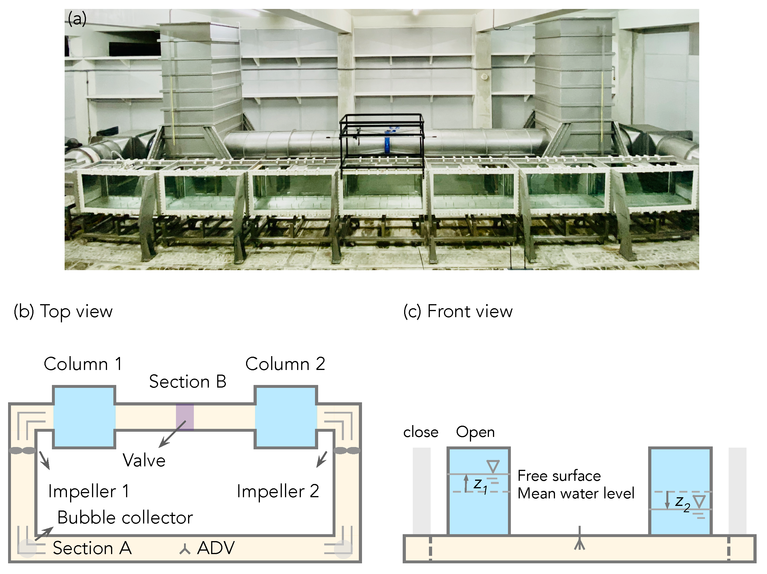
Figure 1 displays the O/U-tube, including a photo and two schematic illustrations. The O/U-tube consisted of two duct sections (Section A and Section B), two vertical columns, two bubble collectors, two impellers, and a valve, as shown in Figure 1b. Section A included the test section, which was 10.5 m long, 0.4 m wide and 0.4 m high with upper lids and a 0.2-m deep sediment pit. The sediment pit could be covered by a flat plate when conducting rigid bed experiments. Deflectors were installed in the four corners. Two honeycomb laminators were installed at each end of the test section to reduce the level of turbulence and scale of the vortices introduced into the test section. The honeycomb comprised stainless steel ducts in the form of a 40 × 40 array. Column 1 and Column 2 were open to the atmosphere and acted as surge tanks to avoid pressure surges. The free water levels in Column 1 and Column 2 ($z_1$ and $z_2$) in Figure 1c changed with the flow velocities in Section A and Section B, respectively. The bubble collectors were cylindrical columns with closed lids, which prevented air bubbles (generated by the two impellers) from moving into the test section. A valve was installed in the middle of Section B. The two impellers were installed in the corners and driven by two 25-kW servomotors. The rotational speed of the motor ranged from −1000 to 1000 revolutions per minute (rpm). The rotation speed of the impeller R could be input into the software to control the rotation of the two impellers. A SonTek acoustic doppler velocimetry (ADV) was installed in the test section to measure the velocity at the centroid of the cross-section. This velocity is the maximum velocity $V_a$ over the cross-section.

3. Hydrodynamics

The hydrodynamic model of the O/U-tube, which is used to analytically examine the hydrodynamic behavior of the O/U-tube with the valve open (referred to as O-tube mode hereafter) and closed (U-tube mode), is presented in this section. Steady flows in O-tube mode and oscillatory flows in U-tube mode were studied.

3.1. Hydrodynamic Model

The equations governing the momentum of the water flow in Section A and Section B are presented as follows:

$$\rho (1+C_{ma})L_a\frac{d{Q}_a}{dt}=\rho g{A}_{ca}(z_1-z_2)-\frac{\rho }{2A_a}{K}_a\left|Q_a\right|Q_a+F_p,$$

(1)

and

$$\rho (1+C_{mb})L_b\frac{d{Q}_b}{dt}=\rho g{A}_{cb}(z_2-z_1)-\frac{\rho }{2A_b}{K}_b\left|Q_b\right|Q_b,$$

(2)

where $L_{a/b}$ is the length of Section A or B, $C_{ma/mb}$ is the model parameter, $Q_{a/b}$ is the flow discharge, $F_p$ is the force applied by the impeller on the water, $K_{a/b}$ is the loss coefficient, $A_{ca/cb}$ is the cross area between the column and section A or B, and $A_{a/b}$ is the representative cross area ($A_{a/b}=L_{a/b}/{\sum }_i^n{L}_i/A_i$). According to the affinity laws [16], $F_p$ and R (rotational speed) have the following relationship:

$$F_p=\frac{\left|R\right|R}{\alpha },$$

(3)

where $\alpha$ is the model parameter. Equations (1) and (2) are similar to the equation in [10] for their O-tube. The first terms on the left-hand side (LHS) of Equations (1) and (2) account for the local inertia force. The resistance force associated with the acceleration is also included in the first terms of $C_{ma}$ and $C_{mb}$, which are excluded from the equation in [10]. $C_{ma}$ and $C_{mb}$ are related to the added mass effect [17] from the deflectors and the honeycomb laminators. The first and second terms on the right-hand side (RHS) of these two equations represent the gravitational and resistance forces, respectively. The major loss (from friction within a pipe) is not considered in the resistance force here, which is generally much smaller than the minor loss (owing to a change in section or other interruption) [17].

The water levels in the two columns are governed by the following mass balance equations:

$$\frac{d{z}_1}{dt}=-\frac{Q_a-Q_b}{A_1},$$

(4)

and

$$\frac{d{z}_2}{dt}=\frac{Q_a-Q_b}{A_2},$$

(5)

where $A_1$ and $A_2$ are the cross-sectional areas of Column 1 and Column 2, respectively.

The volume flow rate $Q_a$ and the fluid velocity $V_a$ (measured by ADV) have the following relationship:

$$V_a=\frac{Q_a}{r{A}_t}$$

(6)

where r is the ratio of the mean velocity to the maximum velocity and $A_t$ is the cross-sectional area of the test section. r depends on the Reynolds number ($Re=V_{a}d/\nu$, with d being the diameter and $\nu$ being the kinematic velocity). For the O/U-tube, $Re$ ranges from ${10}^5$ to ${10}^6$, and r is approximately 0.86 [16].

Equations (1)–(6) were solved numerically using an in-house code based on a simple difference method: the forward Euler method [18]. The time step was 0.01 s. The model parameters are listed in

Table 1. Parameters of the hydrodynamic model.

Parameter	Value	Parameter	Value	Parameter	Value
$C_{ma}$	1.22	$C_{mb}$	0.6	$L_a$	18.35 m
$L_b$	7.5 m	$A_{ca}$	0.33 m2	$A_{cb}$	0.33 m2
$A_a$	0.2 m2	$A_b$	0.33 m2	$A_t$	0.16 m2
$A_{1/2}$	1.21 m2	$K_a$	150 or 120	$K_b$	2
$\alpha$	0.341 rad2/kg m

. The values of $L_a$, $L_b$, $A_{ca}$, $A_{cb}$, $A_a$, $A_b$, and $A_t$ were related to the dimensions of the O/U-tube. $C_{ma}$, $C_{mb}$, $K_a$, $K_b$, and $\alpha$ were obtained through calibration with (1) the conditions $R=100sin(2\pi t/6)$ rpm, $R=200sin(2\pi t/6)$ rpm, and $R=400sin(2\pi t/6)$ rpm using the U-tube mode and (2) the conditions $R=300$ rpm, $R=600$ rpm, $R=100sin(2\pi t/6)$ rpm, and $R=200sin(2\pi t/6)$ rpm using the O-tube mode. The value of $K_a$ is 150 for the U-tube mode and 120 for the O-tube mode. The two modes have different flow structures inside Column 1 and Column 2, yielding a difference in $K_a$. Because the two columns have the same cross area, $A_1=A_2$ is used in the following analysis.

3.2. Steady Flow Conditions with O-Tube Mode

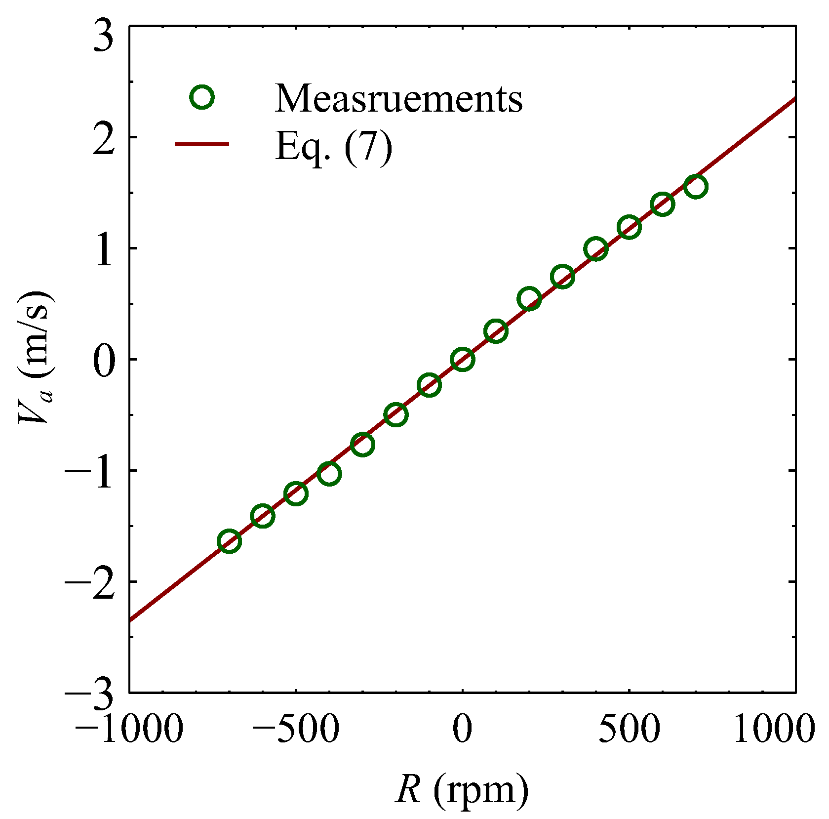
This section examines the steady flow in O-tube mode. Under such conditions, the flow does not change with time; that is, $\partial ·/\partial t=0$. The local inertial force played no role, and the water levels in Column 1 and Column 2 did not change. According to Equations (4) and (5), $Q_a=Q_b$ can be obtained. The combination of Equations (1) and (2) suggests a nonlinear relationship between $F_p$ and $Q_a$ ($F_p=\rho (K_a/A_a+K_b/A_b)\left|Q_a\right|Q_a/2$) because the force applied by the impellers on the water is balanced by the resistance force. According to Equations (3) and (6), the nonlinear relationship can be expressed by the linear relationship between $V_a$ and R:

$$V_a=\sqrt{\frac{{\displaystyle 2}}{{\displaystyle \alpha \rho A_t^2(\frac{K_a}{A_a}+\frac{K_b}{A_b})}}}\frac{{\displaystyle R}}{{\displaystyle r}}.$$

(7)

Figure 2 displays the measured velocity against the rotational speed. The O-tube mode can generate flow with a velocity of up to 1.6 m/s. A linear relationship between $V_a$ and R was observed. Equation (7) was consistent with the measured velocity, thus validating the hydrodynamic model described in Section 3.1. In addition, the O-tube in [10] also revealed a linear relationship between $V_a$ and R in the steady state. Equation (7) can be used to control the impellers to generate a desirable flow velocity for a steady flow or flow with an insignificant local inertial force. For oscillatory flows or flows with a large local inertial force, Equation (7) is not applicable.

3.3. Oscillatory Flow Conditions with the U-Tube Mode

This section describes the hydrodynamics of the U-tube mode with

$$R=R_{1}sin(2\pi t/T)$$

(8)

where $R_1$ is the amplitude and T is the period. The valve is closed and $Q_b=0$. From Equations (1) and (4)–(6), we obtain

$$\rho (1+C_{ma})L_{a}r{A}_t\frac{d{V}_a}{dt}+\frac{\rho }{2A_a}{r}^2{A}_t^2{K}_a\left|V_a\right|V_a+2\rho g\int V_{a}r{A}_{ca}/A_{1}dt=\frac{R^2}{\alpha }.$$

(9)

It is notable that Equations (4) and (5) were integrated with respect to t before being substituted into Equation (1). Again, the first through third terms on the LHS in Equation (9) account for the local inertia force, the resistance force, and the gravitational force. Equation (9) cannot be solved analytically in general. Nondimensionalizing Equation (9) suggests the following three important dimensionless parameters:

$$\begin{array}{ccc}\hfill & {\Pi }_1=\frac{L_a}{TV}=\frac{\mathrm{the}\mathrm{local}\mathrm{inertia}\mathrm{force}}{\mathrm{the}\mathrm{resistance}\mathrm{force}},\hfill & \hfill {\Pi }_2=\frac{L_a}{g{T}^2}=\frac{\mathrm{the}\mathrm{local}\mathrm{inertia}\mathrm{force}}{\mathrm{the}\mathrm{gravitational}\mathrm{force}},\\ \hfill & {\Pi }_3=\frac{gT}{V}=\frac{\mathrm{the}\mathrm{gravitational}\mathrm{force}}{\mathrm{the}\mathrm{resistance}\mathrm{force}}\hfill \end{array}$$

(10)

where V denotes the characteristic velocity. $L_a$ and T are taken as the reference length and the reference time, respectively, in the nondimensionalization process. According to these three dimensionless parameters, the oscillatory flow demonstrates three extreme cases:

• Case I: ${\Pi }_1$ and ${\Pi }_2$ are large.
  In this case, V and T should be small enough. The force applied by the impellers is balanced mainly by the local inertia force. Only the first term on the LHS in Equation (9) is considered; the second and third terms are ignored. In such a situation, the solution to Equations (8) and (9) is given as follows (substituting Equation (8) into Equation (9) and integrating Equation (9) with respect to t):

  $$\begin{array}{cc}\hfill V_a=& \frac{4R_1^{2}T}{3{\pi }^2\alpha \rho (1+C_{ma})L_a{A}_t}\hfill \\ & \left[sin(\frac{{\displaystyle 2\pi t}}{{\displaystyle T}}+\frac{{\displaystyle 3\pi }}{{\displaystyle 2}})+\frac{1}{15}sin(\frac{{\displaystyle 6\pi t}}{{\displaystyle T}}+\frac{{\displaystyle \pi }}{{\displaystyle 2}})+\frac{1}{175}sin(\frac{{\displaystyle 10\pi t}}{{\displaystyle T}}+\frac{{\displaystyle \pi }}{{\displaystyle 2}})+ߪ\right].\hfill \end{array}$$

  (11)
  Equation (11) has been expressed by the Fourier series in amplitude-phase form.
• Case II: ${\Pi }_2$ is small, but ${\Pi }_3$ is large.
  This case occurs when V is small and T is large. The gravitational force dominates. Only the third term on the LHS in Equation (9) is considered when solving Equations (8) and (9) (substituting Equation (8) into Equation (9) and taking derivative of Equation (9)), leading to

  $$\begin{array}{cc}\hfill V_a=& \frac{{\displaystyle 8R_1^2{A}_1}}{{\displaystyle 3A_{ca}{A}_t\alpha \rho grT}}\hfill \\ \hfill & \left[sin(\frac{{\displaystyle 2\pi t}}{{\displaystyle T}}+\frac{{\displaystyle \pi }}{{\displaystyle 2}})+\frac{{\displaystyle 3}}{{\displaystyle 5}}sin(\frac{{\displaystyle 6\pi t}}{{\displaystyle T}}+\frac{{\displaystyle 3\pi }}{{\displaystyle 2}})+\frac{{\displaystyle 1}}{{\displaystyle 7}}sin(\frac{{\displaystyle 10\pi t}}{{\displaystyle T}}+\frac{{\displaystyle 3\pi }}{{\displaystyle 2}})\right].\hfill \end{array}$$

  (12)
  Equation (12) has been expressed by the Fourier series in amplitude-phase form.
• Case III: ${\Pi }_1$ and ${\Pi }_3$ are small.
  This case requires a large V value. In such a case, the resistance dominates the LHS in Equation (9). Only the second term on the LHS in Equation (9) is considered. Therefore, Equations (8) and (9) have the following solution:

  $$V_a=\sqrt{\frac{{\displaystyle 2A_a{R}_1^2}}{{\displaystyle \rho A_t^2{r}^2{K}_a\alpha }}}sin(\frac{{\displaystyle 2\pi t}}{{\displaystyle T}}).$$

  (13)

It can be concluded from Equations (11)–(13) that the three different cases have very different responses of $V_a$ to a simple harmonic rotation of the impellers ($R\sim sin2\pi t/T$), owing to different dominating forces. For Case I and Case II, a simple harmonic rotation of the impellers generates not only the first harmonic component of $V_a$ but also the higher harmonic components ($sin4\pi t/T$, $sin6\pi t/T$, etc.). In these two cases, the flow velocity has a different phase lag with R: $3\pi /2$ for the first harmonic component of Case I and $\pi /2$ for the first harmonic component of Case II. In Case III, the simple harmonic rotation of the impeller does not generate higher harmonic components ir phase lag. Additionally, $V_a$ depends on $R_1^2$ for Case I and Case II but on $R_1$ for Case III. Concerning the effect of T on $V_a$, Case I has a $V_a$ value that is proportional to T, and Case II’s is similar to $1/T$. In Case III, T does not affect $V_a$. In general, the local inertial force, resistance force, and gravitational force have an effect on the flow, and $V_a$ has a more complex response to $R\sim sin2\pi t/T$.

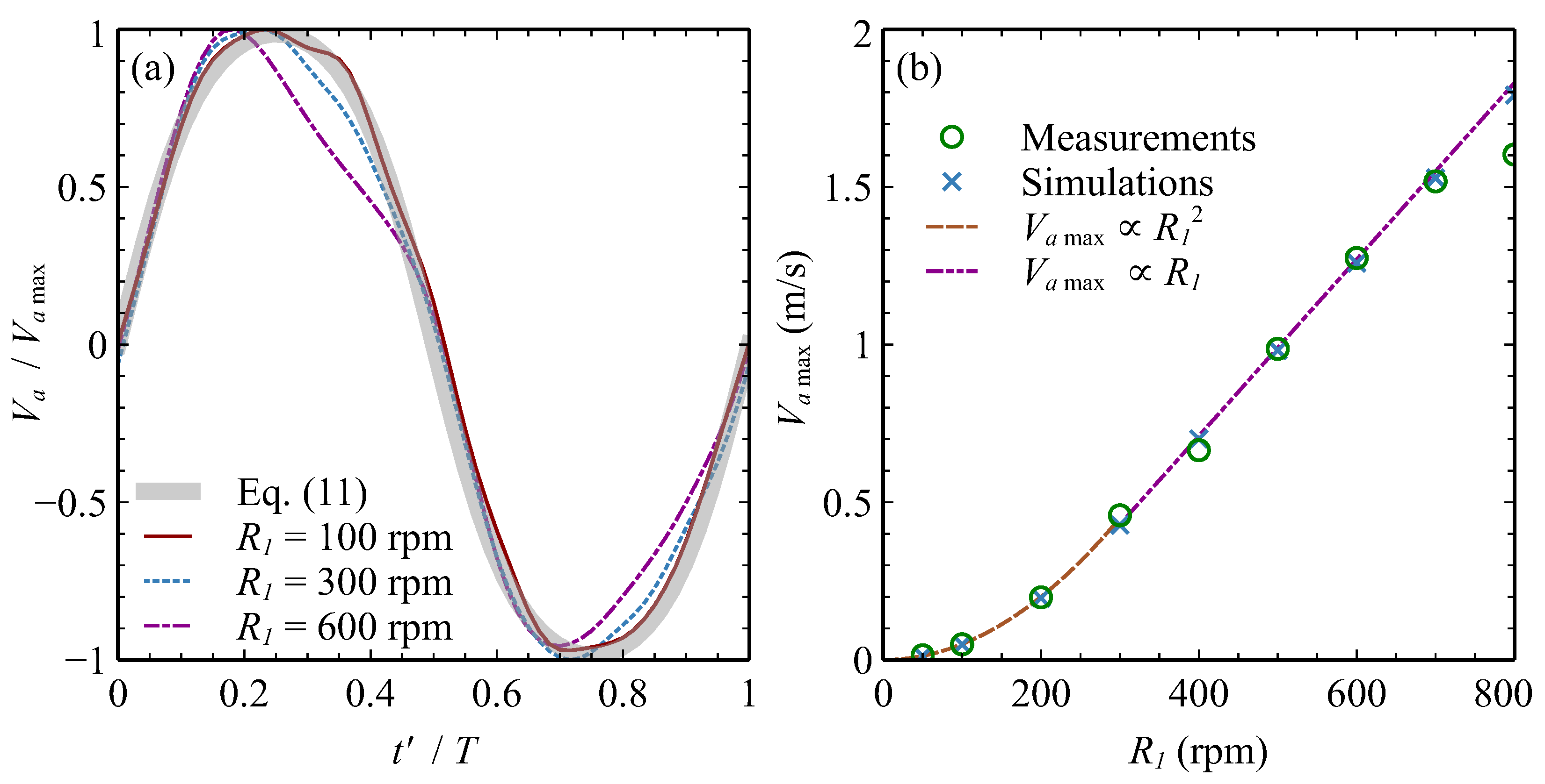
Figure 3 presents the measured velocity with T = 6 s and $R_1$ = 50–800 rpm. Fluctuations in the measured velocity with frequencies of less than 1 s⁻¹ were filtered out. The velocities computed using Equation (11) were superimposed, as shown in Figure 3a. The simulated velocity using the numerical hydrodynamic model presented in Section 3.1 is also shown in Figure 3b. Time in Figure 3a was shifted so that the velocity increased from zero at $t^{\prime }/T=0$, where $t^{\prime }$ is the shifted time. It can be seen in Figure 3a that the time series of velocity for $R_1$ = 100 rpm was close to Equation (11), indicating that the local inertial force dominated when T = 6 s and $R_1$ = 100 rpm. As with $R_1$, the time series deviated from Equation (11) more and more significantly due to the friction force increasing (according to ${\Pi }_1$). As shown in Figure 3b, $V_{a max}$ depends on $R_1^2$ when $R_1$ < 300 rpm but depends on $R_1$ when $R_1$ > 300 rpm. The former relationship also appears in Equation (11) (Case I), and the latter appears in Equation (13) (Case III).

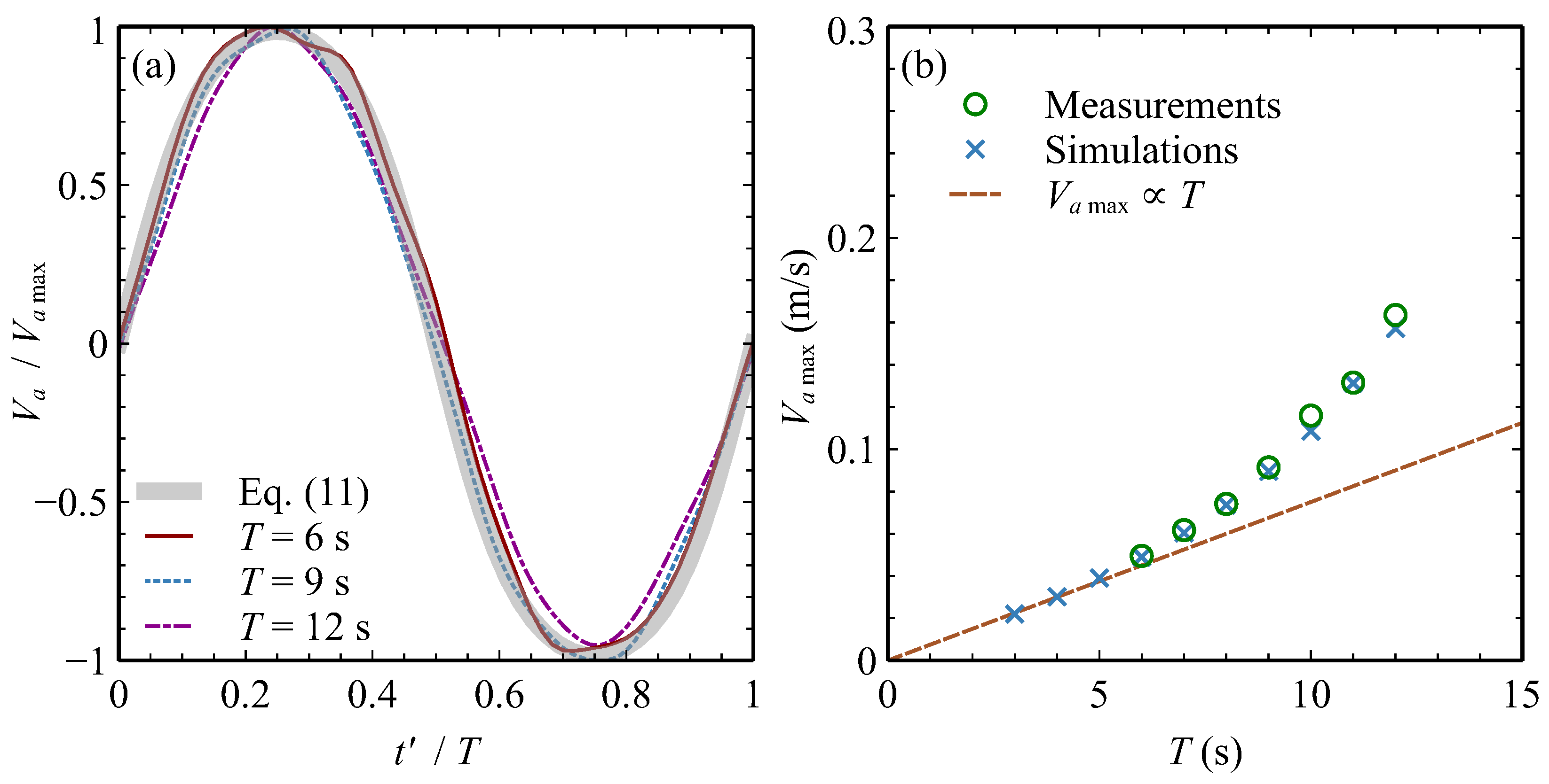
Figure 4 displays the measured velocity for T = 6–12 s and $R_1$ = 100 rpm. As T increased, the gravitational force increased (according to ${\Pi }_2$). Additionally, increasing T increased $V_a$ (see Figure 4), and the friction force also rose (according to ${\Pi }_1$). Therefore, the velocity deviated from Equation (11) with increasing T. With regard to $V_{a max}$, it can be seen in Figure 4b that $V_{a max}$ depended on T only for $T<6$ s as in Equation (11), which also implies that the friction force and gravitational force became increasingly significant with increasing T for $T>6$ s with $R_1$ = 100 rpm.

4. Open-Loop Control

In this section, two open-loop control schemes are developed to generate target flow conditions based on hydrodynamic theory and a genetic algorithm. To generate a steady flow, a simple relationship between the flow velocity and the rotation speed (Equation (7)) can be used. This section focuses on oscillatory flows and considers the target flow velocity as an example:

$$V_a=U_{a}sin(2\pi t/T).$$

(14)

where $U_a$ denotes the amplitude of the oscillating flow velocity. In this section, $U_a$ = 0.6 m/s was considered. Both the U-tube and O-tube modes were examined. An analytical approach was adopted for the U-tube mode, and a numerical approach with a real-valued genetic algorithm was used for the O-tube mode.

4.1. U-Tube: Analytic Approach

Finding the solution $V_a$ in Equation (9) with a given $R\left(t\right)$ is a challenging task, owing to the nonlinearity (the second term on the LHS of Equation (9)). Therefore, only the analytical solutions of $V_a$ for the three extreme cases were obtained in Section 3.3. Here, Equation (9) is solved to find $R\left(t\right)$ for a given $V_a$. In this situation, Equation (9) is a linear equation. The solution of $R\left(t\right)$ is obtained by substituting the target flow velocity $V_a=U_{a}sin(2\pi t/T)$ into Equation (9):

$$R\left(t\right)=\{\begin{array}{cc}\sqrt{\alpha |F_p|},\hfill & \mathrm{if} F_p\ge 0,\\ -\sqrt{\alpha |F_p|},\hfill & \mathrm{if} F_p<0.\end{array}$$

(15)

where

$$\begin{array}{cc}\hfill F_p\left(t\right)=& [{(f_{UI}-f_{UII})}^2+f_{UIII}^2]sin(\frac{{\displaystyle 2\pi t}}{{\displaystyle T}}+\varphi )\hfill \\ \hfill & +\frac{f_{UIII}}{5}sin(\frac{{\displaystyle 6\pi t}}{{\displaystyle T}}+\frac{{\displaystyle \pi }}{{\displaystyle 2}})+\frac{f_{UIII}}{35}sin(\frac{{\displaystyle 10\pi t}}{{\displaystyle T}}+\frac{{\displaystyle \pi }}{{\displaystyle 2}})+...\hfill \end{array}$$

(16)

with

$$\begin{array}{cc}\hfill & f_{UI}=2\pi \rho \pi r{A}_t(1+C_{ma})L_a{U}_a/T,\hfill \\ \hfill & f_{UII}=\rho gr{U}_a{A}_t{A}_{ca}T/A_1\pi ,\hfill \\ \hfill & f_{UIII}=4\rho r^2{U}_a^2{A}_t^2{K}_a/3A_a\pi ,\mathrm{and}\hfill \\ \hfill & \varphi =arctan\left[(f_{UI}-f_{UII})/f_{UIII}\right].\hfill \end{array}$$

(17)

Equation (16) is expressed by a Fourier series with an amplitude-phase form. $f_{UI}$, $f_{UII}$, and $f_{UIII}$ are related to the local inertial, gravitational, and resistance forces, respectively.

Referring to the first term on the RHS of Equation (16), a larger inertia and resistance require a faster rotational speed. The gravitational force (oscillatory water level in Column 1 and Column 2) reduces the required rotational speed. In other words, Column 1 and Column 2 are advantageous for generating a higher oscillatory velocity. The higher harmonic components (the second and third terms on the RHS of Equation (16)) are required to reduce the higher harmonic oscillation of the water due to the resistance force (the second term on the LHS of Equation (9)).

Figure 5 compares the measured velocity and the target velocity. The rotational speed is given by Equations (15)–(17) with $U_a=0.6$ m/s, as shown in Figure 5a. It can be observed in Figure 5 that the R curve lies between the sine wave and the square wave. The measured velocity is extremely close to the target velocity with a slight difference near the trough, possibly because of the fifth-order Fourier series for R adopted here. Overall, it can be concluded that the analytical approach can provide R for generating the target velocity.

4.2. O-Tube: Genetic Algorithm

The hydrodynamics of the O-tube mode involve the flow velocities in Section A and Section B and their phase difference. The complex hydrodynamics prevents the use of an analytical approach to obtain the relationship between the rotational speed and flow velocity.

In this study, a genetic algorithm (GA), which mimics biological evolution, and the numerical hydrodynamic model (NHM), presented in Section 3.1, were used to numerically determine the optimal rotational speed for a target velocity. In this study, the rotational speed is expressed as follows:

$$R\left(t\right)=\frac{R_o^s+{\sum }_{n=1}^6\left[R_n^{s}sin\left(\frac{2n\pi t}{T}+{\gamma }_n^s\right)\right]}{\sqrt{|R_o^s+{\sum }_{n=1}^6\left[R_n^{s}sin\left(\frac{2n\pi t}{T}+{\gamma }_n^s\right)\right]|}}$$

(18)

where $R_o^s$, $R_n^s$, and ${\gamma }_n^s$ with $n=1–6$ are the control parameters in NHM.

According to Equations (3) and (18), $F_p$ is represented by the Fourier series. It is expected to generate any desired periodic oscillatory flow by changing these control parameters. These 13 parameters are the genes in the GA, and they constitute the chromosome using real value representation (genes are represented by real values but not binary values). Each population contained 60 chromosomes. The objective of the GA scheme is to allow the population to evolve such that the next population has a better fit of the computed velocity to the target velocity. The fitness (F) is defined as follows:

$$F=\frac{1}{\sqrt{{\int }_0^T{(V_c-V_t)}^2/Tdt}}$$

(19)

For the initial population, 13 parameters were initialized randomly within reasonable ranges for each chromosome. The GA performs the following steps to generate the subsequent population:

• Performing the tournament selection with a tournament size of three. Three chromosomes from the current generation were selected, and the fittest among them became the parent chromosome.
• Conducting the blend crossover with a crossover rate of one. Two offspring chromosomes received random values anywhere between the mother’s chromosome and the father’s chromosome.
• Accomplishing uniform mutation with a mutation rate of 0.4. All possible values were equally probable for the mutated gene.
• We repeated Steps 1–3 until the population size was big enough (60).
• Performing elitism. We compared the fineness of all the generated chromosomes and all the previous chromosomes, selecting the top 50% chromosomes according to the fitness as the next population.
• Steps 1–5 were repeated 60 times.

The GA parameters are summarized in

Table 2. GA parameters.

GA Parameters	Setting Values
Code method	Real coded
Population size	60
Generation	60
Selection	Tournament selection
Crossover algorithm	Blend crossover
Crossover rate	1.0
Mutation algorithm	Uniform mutation
Mutation rate	0.4
Elitism	Yes

. The obtained optimal parameters for generating the target velocity were $R_o^s=0{\mathrm{rpm}}^2$, $R_1^s=\mathrm{103,658.01}{\mathrm{rpm}}^2$, $R_2^s=1881.15{\mathrm{rpm}}^2$, $R_3^s=2332.82{\mathrm{rpm}}^2$, $R_4^s=1359.39{\mathrm{rpm}}^2$, $R_5^s=1461.68{\mathrm{rpm}}^2$, $R_6^s=1393.45{\mathrm{rpm}}^2$, ${\gamma }_1^s=0.8$, ${\gamma }_2^s=2.45$, ${\gamma }_3^s=2.38$, ${\gamma }_4^s=2.17$, ${\gamma }_5^s=2.1$, and ${\gamma }_6^s=2.2$. The fitness was approximately 80. These values were used in the O-tube mode to generate flow.

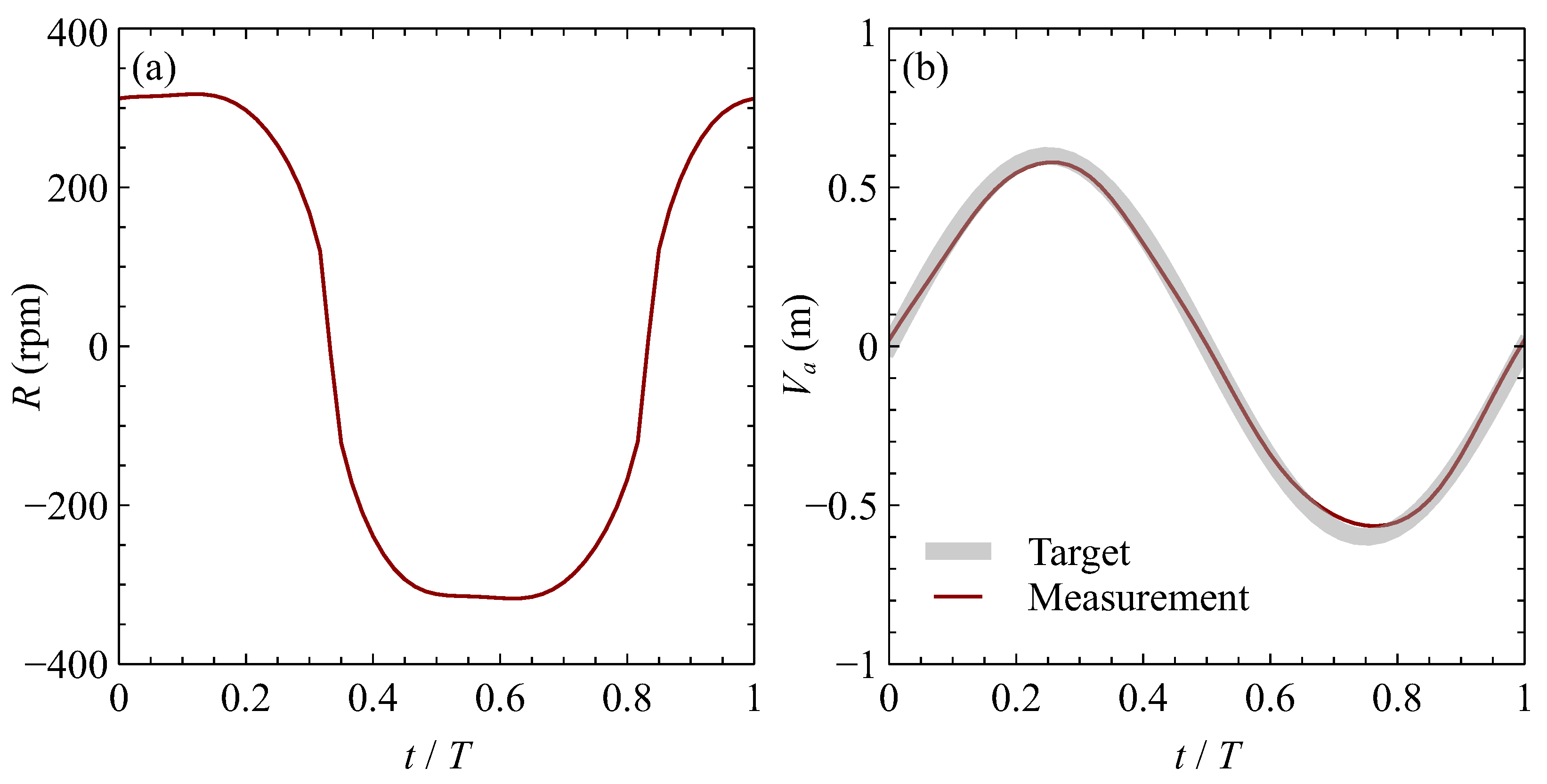
Figure 6 displays the rotational speed and the flow velocity in O-tube mode, including the target velocity, measured velocity, and the simulated velocity. It can be observed in Figure 6a that $R\left(t\right)$ is between the sine wave and the square wave. Compared with U-tube mode (Figure 5), O-tube mode had a sharper crest and trough on the $R\left(t\right)$ curve. The rotational speed shown in Figure 6b provided a measured $V_a$ close to the target velocity. The simulated velocity agreed well with the measured velocity. It can be concluded that the GA and NHM can suggest appropriate $R_n^s$ and ${\gamma }_n^s$ values to generate the target velocity.

5. Conclusions

This study introduced an O/U-tube (new oscillatory water tunnel) which drove the flow using two impellers. The O/U-tube can be reduced to U-tube mode (generating an oscillatory flow) or O-tube mode (generating both an oscillatory flow and a unidirectional flow with a flow velocity of up to 1.6 m/s). The hydrodynamic analysis indicates that the local inertia, gravity, and resistance forces caused different responses by the flow velocity to the sine-varying rotational speed of the impeller in U-tube mode. The local inertia and gravity forces yielded higher harmonic components for the velocity. For the steady state of the O-tube mode, hydrodynamic analysis suggests a linear relationship between the flow and rotational speed, which is consistent with the experimental observations. Two open-loop control schemes are proposed to generate the target flow conditions: the analytic approach for U-tube mode and the genetic algorithm for O-tube mode. The analytic approach determines the rotational speed by solving the momentum balance equations with a given velocity. In the genetic algorithm, the rotational speed is represented by a square root of the Fourier series. The optimal coefficients of the Fourier series to generate the target flow were determined by using the genetic algorithm and a hydrodynamic model. Experiments were conducted to validate the two open-loop control schemes. The O/U-tube with the open-loop control schemes can generate the desired oscillatory flows and unidirectional flows. In future, the O/U-tube will be used to investigate turbulence characteristics and sediment transport under various oscillatory flow and unidirectional flow conditions.

References

- Fredsoe, J.; Deigaard, R. Mechanics of Coastal Sediment Transport; World Scientific: Singapore, 1994. [Google Scholar]
- Nielsen, P. Coastal Bottom Boundary Layers and Sediment Transport; World Scientific: Singapore, 1992. [Google Scholar]
- Dean, R.G.; Dalrymple, R.A. Coastal Processes with Engineering Applications; Cambridge University Press: Cambridge, UK, 2006. [Google Scholar]
- Daily, J.W. The Water Tunnel as a Tool in Hydraulic Research. In Proceedings of the Third Hydraulics Conference, Iowa City, IA, USA, 10–12 June 1947; pp. 169–189. [Google Scholar]
- López de San Román-Blanco, B.; Coates, T.T.; Holmes, P.; Chadwick, A.J.; Bradbury, A.; Baldock, T.E.; Pedrozo-Acuña, A.; Lawrence, J.; Grüne, J. Large scale experiments on gravel and mixed beaches: Experimental procedure, data documentation and initial results. Coast. Eng. 2006, 53, 349–362. [Google Scholar] [CrossRef]
- Zhang, H.; Geng, B. Introduction of the world largest wave flume constructed by TIWTE. Procedia Eng. 2015, 116, 905–911. [Google Scholar] [CrossRef] [Green Version]
- Hsu, W.Y.; Huang, Z.C.; Na, B.; Chang, K.A.; Chuang, W.L.; Yang, R.Y. Laboratory Observation of Turbulence and Wave Shear Stresses Under Large Scale Breaking Waves Over a Mild Slope. J. Geophys. Res. 2019, 124, 7486–7512. [Google Scholar] [CrossRef]
- Ribberink, J.S.; Al-Salem, A.A. Sediment transport in oscillatory boundary layers in cases of rippled beds and sheet flow. J. Geophys. Res. 1994, 99, 12707–12727. [Google Scholar] [CrossRef]
- Yuan, J.; Madsen, O.S. Experimental study of turbulent oscillatory boundary layers in an oscillating water tunnel. Coast. Eng. 2014, 89, 63–84. [Google Scholar] [CrossRef]
- Mohr, H.; Draper, S.; White, D.J.; Cheng, L.; An, H.; Zhang, Q. The hydrodynamics of a recirculating (O-tube) flume. In Proceedings of the Scour and Erosion-Proceedings of the 8th International Conference on Scour and Erosion, ICSE 2016, Oxford, UK, 12–15 September 2016; pp. 999–1010. [Google Scholar]
- An, H.; Luo, C.; Cheng, L.; White, D. A new facility for studying ocean-structure–seabed interactions: The O-tube. Coast. Eng. 2013, 82, 88–101. [Google Scholar] [CrossRef]
- Yang, Z.; Huang, B.; Kang, A.; Zhu, B.; Han, J.; Yin, R.; Li, X. Experimental study on the solitary wave-current interaction and the combined forces on a vertical cylinder. Ocean Eng. 2021, 236. [Google Scholar] [CrossRef]
- Van der Werf, J.J.; Schretlen, J.J.; Ribberink, J.S.; O’Donoghue, T. Database of full-scale laboratory experiments on wave-driven sand transport processes. Coast. Eng. 2009, 56, 726–732. [Google Scholar] [CrossRef]
- Wurbs, R.; James, W. Water Resources Engineering; Pearson Education Taiwan Ltd.: Taipei, Taiwan, 2002. [Google Scholar]
- Katoch, S.; Chauhan, S.S.; Kumar, V. A review on genetic algorithm: Past, present, and future. In Multimedia Tools and Applications; Springer: New York, NY, USA, 2021; Volume 80, pp. 8091–8126. [Google Scholar]
- White, F. Fluid Mechanics; McGraw-Hill: New York, NY, USA, 2010. [Google Scholar]
- Lamb, H. Hydrodynamics, 6th ed.; Dover Publications: New York, NY, USA, 1945. [Google Scholar]
- Ferziger, J.H.; Peric, M. Computational Methods for Fluid Dynamics; Springer: Berlin, Germany, 2002. [Google Scholar]
Figure 1.
The O/U-tube. (a) Photo. Schematic illustration: (b) top view and (c) front view.
Figure 2.
Flow velocity against rotational speed with the O-tube mode under steady state conditions.
Figure 3.
(a) Measured time series of flow velocity () for T = 6 s and = 100, 300, and 600 rpm with U-tube mode. (b) The maximum velocity against from the experiments and simulations.
Figure 4.
(a) Measured time series of flow velocity () for T = 6, 9, and 12 s and = 100, 300, and 600 rpm with U-tube mode. (b) The maximum velocity against from the experiments and simulations.
Figure 5.
(a) Time series of rotational speed. (b) Time series of velocity using the U-tube model.
Figure 6.
(a) Time series of rotational speed. (b) Time series of velocity using O-tube mode.