
Estimating the Standardized Precipitation Evapotranspiration Index Using Data-Driven Techniques: A Regional Study of Bangladesh

 ,
,  ,
,  , , ,
, , ,  , and
, and
Abstract
:1. Introduction
2. Materials and Methods
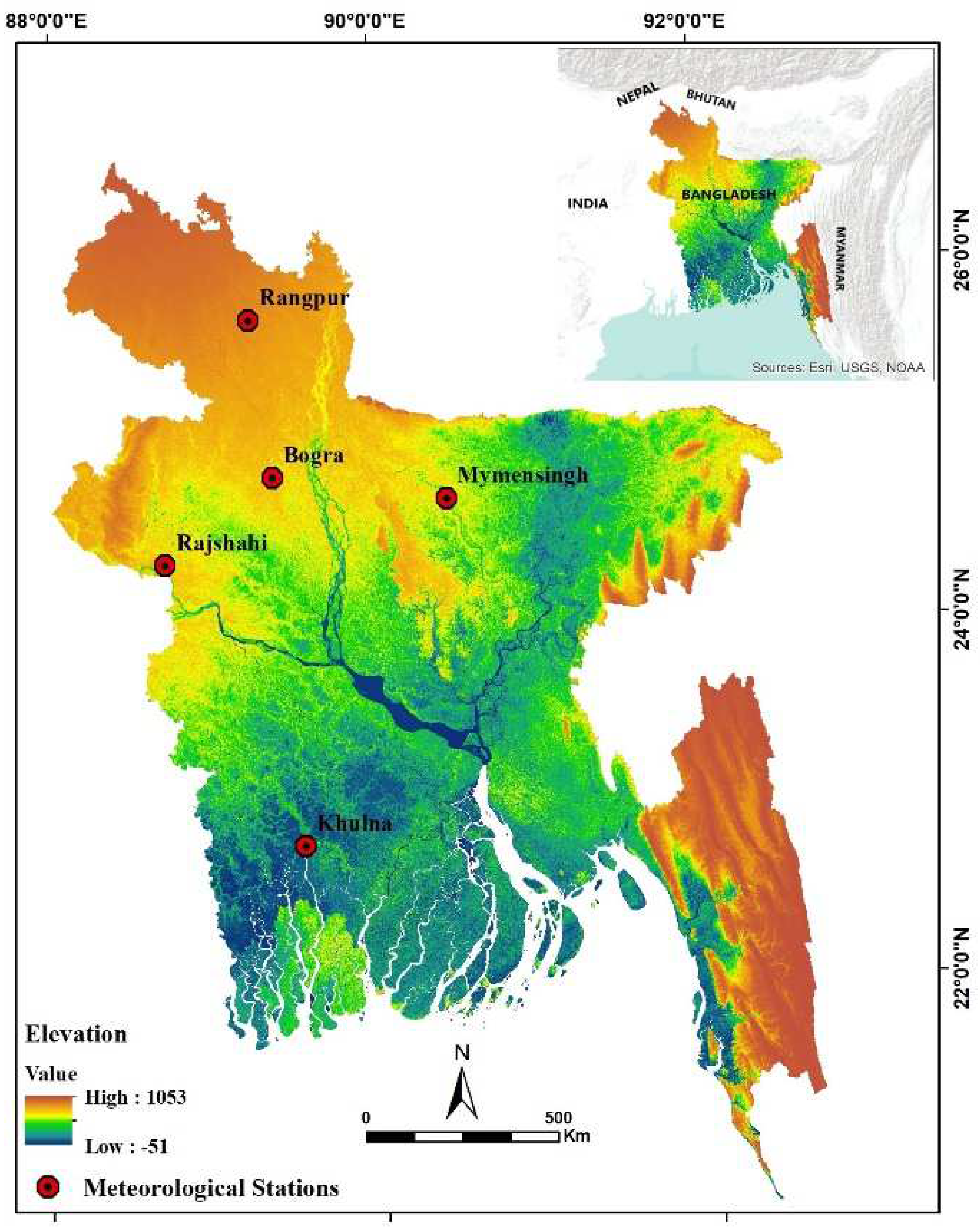
2.1. Study Area
2.2. Data
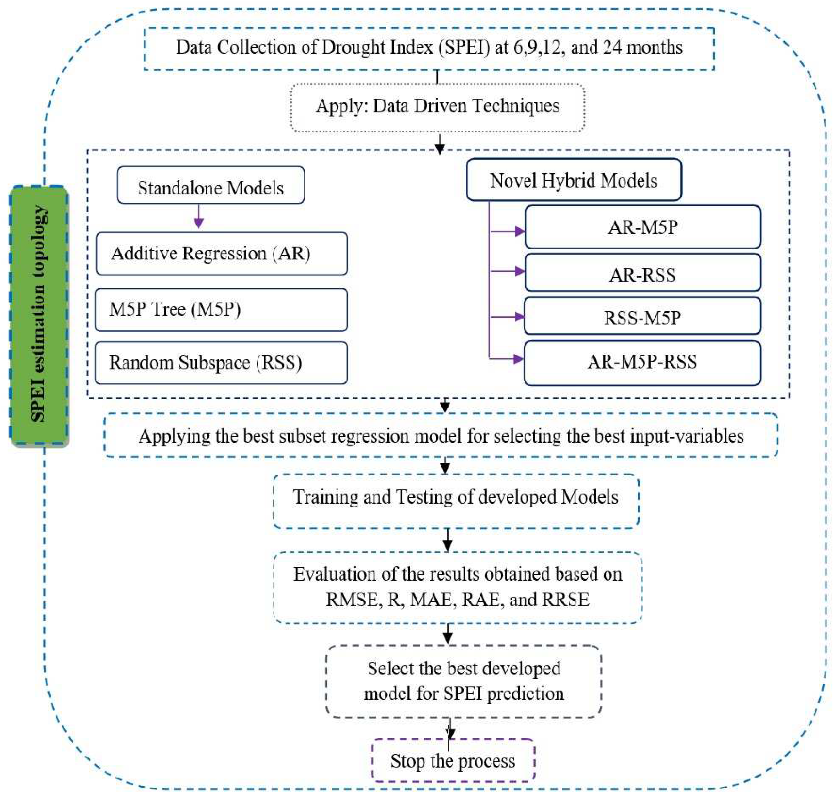
2.3. Methodology
2.3.1. SPEI Calculation
2.3.2. Machine Learning Algorithms
2.4. Constructing and Evaluating Models
2.5. Statistical Performance Measurement
3. Results
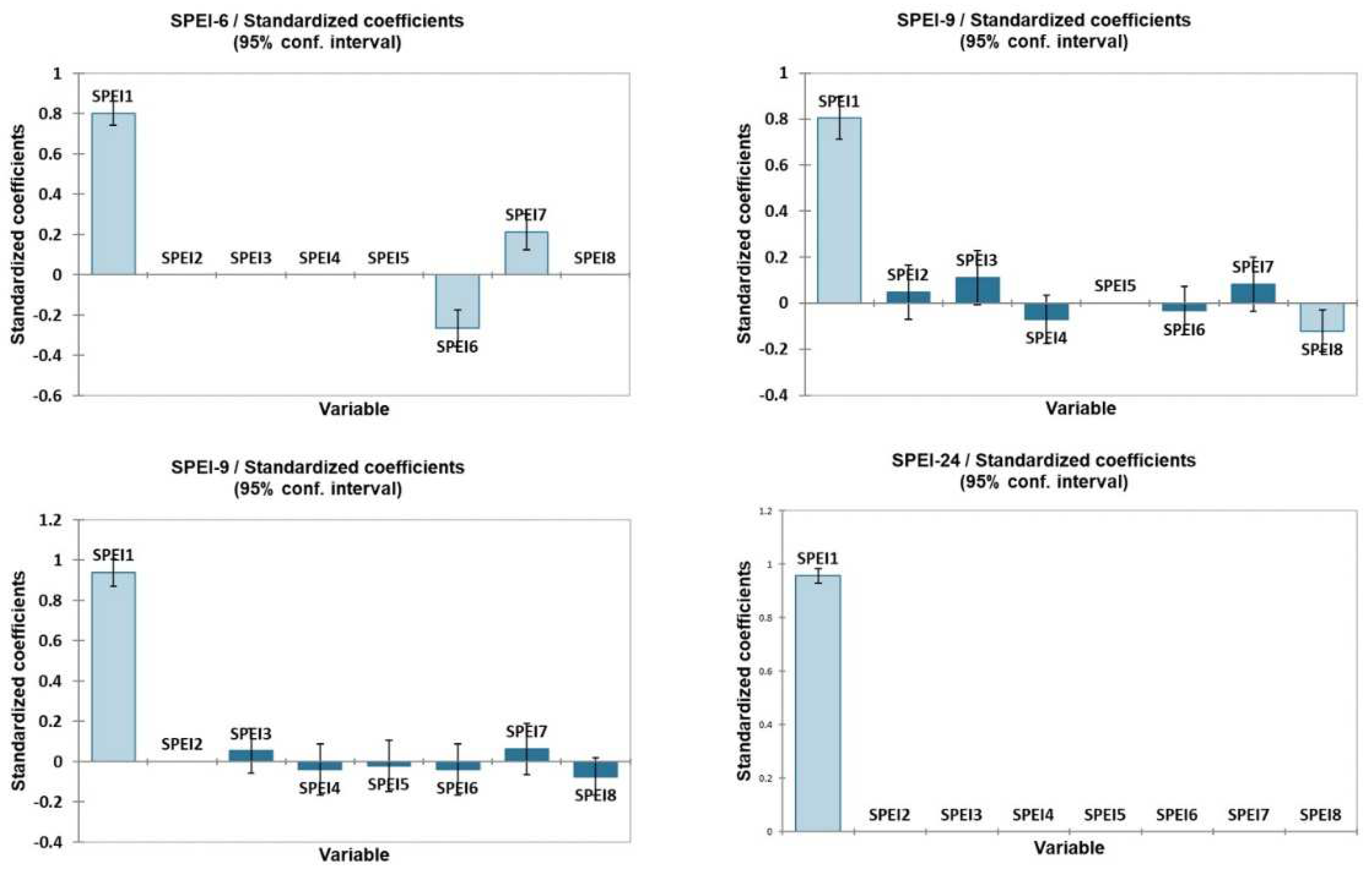
3.1. Model Input Selection
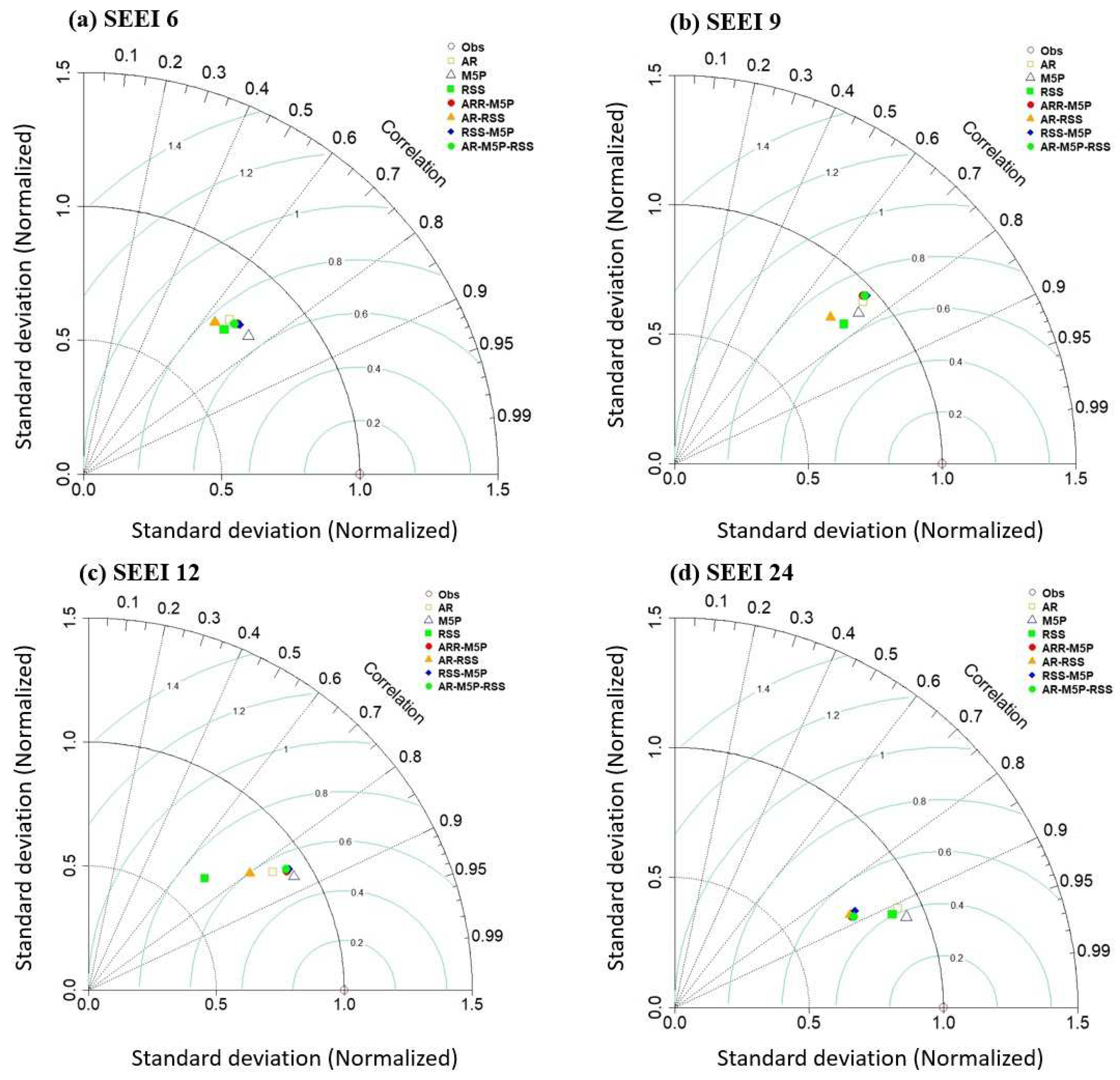
3.2. Prediction of Droughts Using Machine Learning Techniques
3.3. The Best Predictive Model Is Applied in Various Regions
4. Discussion
5. Conclusions
Author Contributions
Funding
Institutional Review Board Statement
Informed Consent Statement
Data Availability Statement
Conflicts of Interest
References
- Kamruzzaman, M.; Hwang, S.; Cho, J.; Jang, M.W.; Jeong, H. Evaluating the Spatiotemporal Characteristics of Agricultural Drought in Bangladesh Using Effective Drought Index. Water 2019, 11, 2437. [Google Scholar] [CrossRef] [Green Version]
- Kamruzzaman, M.; Jang, M.-W.W.; Cho, J.; Hwang, S. Future Changes in Precipitation and Drought Characteristics over Bangladesh under CMIP5 Climatological Projections. Water 2019, 11, 2219. [Google Scholar] [CrossRef] [Green Version]
- Lorenzo-Lacruz, J.; Vicente-Serrano, S.M.; López-Moreno, J.I.; Beguería, S.; García-Ruiz, J.M.; Cuadrat, J.M. The Impact of Droughts and Water Management on Various Hydrological Systems in the Headwaters of the Tagus River (Central Spain). J. Hydrol. 2010, 386, 13–26. [Google Scholar] [CrossRef] [Green Version]
- Potop, V.; Možný, M.; Soukup, J. Drought Evolution at Various Time Scales in the Lowland Regions and Their Impact on Vegetable Crops in the Czech Republic. Agric. For. Meteorol. 2012, 156, 121–133. [Google Scholar] [CrossRef]
- Qin, Y.; Yang, D.; Lei, H.; Xu, K.; Xu, X. Comparative Analysis of Drought Based on Precipitation and Soil Moisture Indices in Haihe Basin of North China during the Period of 1960–2010. J. Hydrol. 2015, 526, 55–67. [Google Scholar] [CrossRef]
- Yang, X.; Zheng, W.; Lin, C.; Ren, L.; Wang, Y.; Zhang, M.; Yuan, F.; Jiang, S. Prediction of Drought in the Yellow River Based on Statistical Downscale Study and SPI. J. Hohai Univ. 2017, 45, 377. [Google Scholar] [CrossRef]
- Alamgir, M.; Shahid, S.; Hazarika, M.K.; Nashrrullah, S.; Harun, S.B.; Shamsudin, S. Analysis of Meteorological Drought Pattern during Different Climatic and Cropping Seasons in Bangladesh. J. Am. Water Resour. Assoc. 2015, 51, 794–806. [Google Scholar] [CrossRef]
- Islam, A.R.M.T.; Salam, R.; Yeasmin, N.; Kamruzzaman, M.; Shahid, S.; Fattah, M.A.; Uddin, A.S.; Shahariar, M.H.; Mondol, M.A.H.; Jhajharia, D.; et al. Spatiotemporal Distribution of Drought and Its Possible Associations with ENSO Indices in Bangladesh. Arab. J. Geosci. 2021, 14, 2681. [Google Scholar] [CrossRef]
- Fahad, M.G.R.; Saiful Islam, A.K.M.; Nazari, R.; Alfi Hasan, M.; Tarekul Islam, G.M.; Bala, S.K. Regional Changes of Precipitation and Temperature over Bangladesh Using Bias-Corrected Multi-Model Ensemble Projections Considering High-Emission Pathways. Int. J. Climatol. 2018, 38, 1634–1648. [Google Scholar] [CrossRef]
- Dai, A. Characteristics and Trends in Various Forms of the Palmer Drought Severity Index during 1900–2008. J. Geophys. Res. Atmos. 2011, 116. [Google Scholar] [CrossRef] [Green Version]
- Dai, A. Increasing Drought under Global Warming in Observations and Models. Nat. Clim. Chang. 2013, 3, 52–58. [Google Scholar] [CrossRef]
- Aadhar, S.; Mishra, V. On the Occurrence of the Worst Drought in South Asia in the Observed and Future Climate. Environ. Res. Lett. 2021, 16, 024050. [Google Scholar] [CrossRef]
- Hao, Z.; Singh, V.P.; Xia, Y. Seasonal Drought Prediction: Advances, Challenges, and Future Prospects. Rev. Geophys. 2018, 56, 108–141. [Google Scholar] [CrossRef] [Green Version]
- Mishra, A.K.; Singh, V.P. Drought Modeling—A Review. J. Hydrol. 2011, 403, 157–175. [Google Scholar] [CrossRef]
- Shahid, S. Rainfall Variability and the Trends of Wet and Dry Periods in Bangladesh. Int. J. Climatol. 2010, 30, 2299–2313. [Google Scholar] [CrossRef]
- Pozzi, W.; Sheffield, J.; Stefanski, R.; Cripe, D.; Pulwarty, R.; Vogt, J.V.; Heim, R.R.; Brewer, M.J.; Svoboda, M.; Westerhoff, R.; et al. Toward Global Drought Early Warning Capability: Expanding International Cooperation for the Development of a Framework for Monitoring and Forecasting. Bull. Am. Meteorol. Soc. 2013, 94, 776–785. [Google Scholar] [CrossRef]
- Yaseen, Z.M.; El-shafie, A.; Jaafar, O.; Afan, H.A.; Sayl, K.N. Artificial Intelligence Based Models for Stream-Flow Forecasting: 2000–2015. J. Hydrol. 2015, 530, 829–844. [Google Scholar] [CrossRef]
- Turco, M.; Ceglar, A.; Prodhomme, C.; Soret, A.; Toreti, A.; Doblas-Reyes Francisco, J. Summer Drought Predictability over Europe: Empirical versus Dynamical Forecasts. Environ. Res. Lett. 2017, 12, 084006. [Google Scholar] [CrossRef] [Green Version]
- Murakami, H.; Villarini, G.; Vecchi, G.A.; Zhang, W.; Gudgel, R. Statistical-Dynamical Seasonal Forecast of North Atlantic and U.S. Landfalling Tropical Cyclones Using the High-Resolution GFDL FLOR Coupled Model. Mon. Weather Rev. 2016, 144, 2101–2123. [Google Scholar] [CrossRef]
- Strazzo, S.; Collins, D.C.; Schepen, A.; Wang, Q.J.; Becker, E.; Jia, L. Application of a Hybrid Statistical-Dynamical System to Seasonal Prediction of North American Temperature and Precipitation. Mon. Weather Rev. 2019, 147, 607–625. [Google Scholar] [CrossRef]
- Madadgar, S.; AghaKouchak, A.; Shukla, S.; Wood, A.W.; Cheng, L.; Hsu, K.L.; Svoboda, M. A Hybrid Statistical-Dynamical Framework for Meteorological Drought Prediction: Application to the Southwestern United States. Water Resour. Res. 2016, 52, 5095–5110. [Google Scholar] [CrossRef] [Green Version]
- Belayneh, A.; Adamowski, J.; Khalil, B.; Quilty, J. Coupling Machine Learning Methods with Wavelet Transforms and the Bootstrap and Boosting Ensemble Approaches for Drought Prediction. Atmos. Res. 2016, 172–173, 37–47. [Google Scholar] [CrossRef]
- Ganguli, P.; Janga Reddy, M. Ensemble Prediction of Regional Droughts Using Climate Inputs and the SVM-Copula Approach. Hydrol. Process. 2014, 28, 4989–5009. [Google Scholar] [CrossRef]
- Mariotti, A.; Schubert, S.; Mo, K.; Peters-Lidard, C.; Wood, A.; Pulwarty, R.; Huang, J.; Barrie, D. Advancing Drought Understanding, Monitoring, and Prediction. Bull. Am. Meteorol. Soc. 2013, 94, ES186–ES188. [Google Scholar] [CrossRef]
- Xu, L.; Chen, N.; Zhang, X.; Chen, Z. An Evaluation of Statistical, NMME and Hybrid Models for Drought Prediction in China. J. Hydrol. 2018, 566, 235–249. [Google Scholar] [CrossRef] [Green Version]
- Chatterjee, I. Patenting Machine-Learning: Review and Discussions. Int. J. Mod. Res. 2021, 1, 15–21. [Google Scholar]
- Kumar Vaishnav, P.; Sharma, S.; Sharma, P. Analytical Review Analysis for Screening COVID-19 Disease. Int. J. Mod. Res. 2021, 1, 22–29. [Google Scholar]
- Kumar, R.; Dhiman, G. A Comparative Study of Fuzzy Optimization through Fuzzy Number. Int. J. Mod. Res. 2021, 1, 1–14. [Google Scholar]
- Sachindra, D.A.; Kanae, S. Machine Learning for Downscaling: The Use of Parallel Multiple Populations in Genetic Programming. Stoch. Environ. Res. Risk Assess. 2019, 33, 1497–1533. [Google Scholar] [CrossRef] [Green Version]
- Parmar, A.; Mistree, K.; Sompura, M. Machine Learning Techniques For Rainfall Prediction: A Review. In Proceedings of the 2017 International Conference on Innovations in information Embedded and Communication Systems (ICIIECS), Coimbatore, India, 17–18 March 2017. [Google Scholar]
- Tian, Y.; Xu, Y.P.; Wang, G. Agricultural Drought Prediction Using Climate Indices Based on Support Vector Regression in Xiangjiang River Basin. Sci. Total Environ. 2018, 622–623, 710–720. [Google Scholar] [CrossRef]
- Khan, N.; Shahid, S.; Juneng, L.; Ahmed, K.; Ismail, T.; Nawaz, N. Prediction of Heat Waves in Pakistan Using Quantile Regression Forests. Atmos. Res. 2019, 221, 1–11. [Google Scholar] [CrossRef]
- Fung, K.F.; Huang, Y.F.; Koo, C.H.; Soh, Y.W. Drought Forecasting: A Review of Modelling Approaches 2007–2017. J. Water Clim. Change 2020, 11, 771–799. [Google Scholar] [CrossRef]
- Malik, A.; Kumar, A.; Salih, S.Q.; Kim, S.; Kim, N.W.; Yaseen, Z.M.; Singh, V.P. Drought Index Prediction Using Advanced Fuzzy Logic Model: Regional Case Study over Kumaon in India. PLoS ONE 2020, 15, e0233280. [Google Scholar] [CrossRef] [PubMed]
- Kisi, O.; Choubin, B.; Deo, R.C.; Yaseen, Z.M. Incorporating Synoptic-Scale Climate Signals for Streamflow Modelling over the Mediterranean Region Using Machine Learning Models. Hydrol. Sci. J. 2019, 64, 1240–1252. [Google Scholar] [CrossRef]
- Rhee, J.; Im, J. Meteorological Drought Forecasting for Ungauged Areas Based on Machine Learning: Using Long-Range Climate Forecast and Remote Sensing Data. Agric. For. Meteorol. 2017, 237–238, 105–122. [Google Scholar] [CrossRef]
- Mouatadid, S.; Deo, R.C.; Adamowski, J.F. Prediction of SPEI Using MLR and ANN: A Case Study for Wilsons Promontory Station in Victoria. In Proceedings of the 2015 IEEE 14th International Conference on Machine Learning and Applications, ICMLA 2015, Miami, FL, USA, 9–11 December 2015. [Google Scholar]
- Mouatadid, S.; Raj, N.; Deo, R.C.; Adamowski, J.F. Input Selection and Data-Driven Model Performance Optimization to Predict the Standardized Precipitation and Evaporation Index in a Drought-Prone Region. Atmos. Res. 2018, 212, 130–149. [Google Scholar] [CrossRef]
- Park, S.; Im, J.; Jang, E.; Rhee, J. Drought Assessment and Monitoring through Blending of Multi-Sensor Indices Using Machine Learning Approaches for Different Climate Regions. Agric. For. Meteorol. 2016, 216, 157–169. [Google Scholar] [CrossRef]
- Belayneh, A.; Adamowski, J.; Khalil, B.; Ozga-Zielinski, B. Long-Term SPI Drought Forecasting in the Awash River Basin in Ethiopia Using Wavelet Neural Networks and Wavelet Support Vector Regression Models. J. Hydrol. 2014, 508, 418–429. [Google Scholar] [CrossRef]
- Deo, R.C.; Şahin, M. Application of the Artificial Neural Network Model for Prediction of Monthly Standardized Precipitation and Evapotranspiration Index Using Hydrometeorological Parameters and Climate Indices in Eastern Australia. Atmos. Res. 2015, 161–162, 65–81. [Google Scholar] [CrossRef]
- Deo, R.C.; Kisi, O.; Singh, V.P. Drought Forecasting in Eastern Australia Using Multivariate Adaptive Regression Spline, Least Square Support Vector Machine and M5Tree Model. Atmos. Res. 2017, 184, 149–175. [Google Scholar] [CrossRef] [Green Version]
- Mokhtar, A.; Jalali, M.; He, H.; Al-Ansari, N.; Elbeltagi, A.; Alsafadi, K.; Abdo, H.G.; Sammen, S.S.; Gyasi-Agyei, Y.; Rodrigo-Comino, J. Estimation of SPEI Meteorological Drought Using Machine Learning Algorithms. IEEE Access 2021, 9, 65503–65523. [Google Scholar] [CrossRef]
- Yaseen, Z.M.; Ali, M.; Sharafati, A.; Al-Ansari, N.; Shahid, S. Forecasting Standardized Precipitation Index Using Data Intelligence Models: Regional Investigation of Bangladesh. Sci. Rep. 2021, 11, 3435. [Google Scholar] [CrossRef]
- Mehdizadeh, S.; Ahmadi, F.; Danandeh Mehr, A.; Safari, M.J.S. Drought Modeling Using Classic Time Series and Hybrid Wavelet-Gene Expression Programming Models. J. Hydrol. 2020, 587, 125017. [Google Scholar] [CrossRef]
- Ali, M.; Deo, R.C.; Maraseni, T.; Downs, N.J. Improving SPI-Derived Drought Forecasts Incorporating Synoptic-Scale Climate Indices in Multi-Phase Multivariate Empirical Mode Decomposition Model Hybridized with Simulated Annealing and Kernel Ridge Regression Algorithms. J. Hydrol. 2019, 576, 164–184. [Google Scholar] [CrossRef]
- Danandeh Mehr, A.; Kahya, E.; Özger, M. A Gene-Wavelet Model for Long Lead Time Drought Forecasting. J. Hydrol. 2014, 517, 691–699. [Google Scholar] [CrossRef]
- Anshuka, A.; van Ogtrop, F.F.; Willem Vervoort, R. Drought Forecasting through Statistical Models Using Standardised Precipitation Index: A Systematic Review and Meta-Regression Analysis. Nat. Hazards 2019, 97, 955–977. [Google Scholar] [CrossRef]
- Zhang, R.; Chen, Z.Y.; Xu, L.J.; Ou, C.Q. Meteorological Drought Forecasting Based on a Statistical Model with Machine Learning Techniques in Shaanxi Province, China. Sci. Total Environ. 2019, 665, 338–346. [Google Scholar] [CrossRef]
- Ozger, M.; Mishra, A.K.; Singh, V.P. Estimating Palmer Drought Severity Index Using a Wavelet Fuzzy Logic Model Based on Meteorological Variables. Int. J. Climatol. 2011, 31, 2021–2032. [Google Scholar] [CrossRef]
- Masinde, M. Artificial Neural Networks Models for Predicting Effective Drought Index: Factoring Effects of Rainfall Variability. Mitig. Adapt. Strateg. Glob. Chang. 2014, 19, 1139–1162. [Google Scholar] [CrossRef]
- Prasad, R.; Deo, R.C.; Li, Y.; Maraseni, T. Input Selection and Performance Optimization of ANN-Based Streamflow Forecasts in the Drought-Prone Murray Darling Basin Region Using IIS and MODWT Algorithm. Atmos. Res. 2017, 197, 42–63. [Google Scholar] [CrossRef]
- Liang, Z.; Li, Y.; Hu, Y.; Li, B.; Wang, J. A Data-Driven SVR Model for Long-Term Runoff Prediction and Uncertainty Analysis Based on the Bayesian Framework. Theor. Appl. Climatol. 2018, 133, 137–149. [Google Scholar] [CrossRef]
- Bagmar, M.S.H.; Khudri, M.M. Application of Box-Jenkins Models for Forecasting Drought in North-Western Part of Bangladesh. Environ. Eng. Res. 2021, 26, 200294. [Google Scholar] [CrossRef]
- Habiba, U.; Shaw, R.; Takeuchi, Y. Farmers’ Adaptive Practices for Drought Risk Reduction in the Northwest Region of Bangladesh. Nat. Hazards 2014, 72, 337–359. [Google Scholar] [CrossRef]
- Shahid, S.; Behrawan, H. Drought Risk Assessment in the Western Part of Bangladesh. Nat. Hazards 2008, 46, 391–413. [Google Scholar] [CrossRef]
- Paul, B.K. Coping Mechanisms Practised by Drought Victims (1994/5) in North Bengal, Bangladesh. Appl. Geogr. 1998, 18, 355–373. [Google Scholar] [CrossRef]
- Kamruzzaman, M.; Cho, J.; Jang, M.-W.; Hwang, S. Comparative Evaluation of Standardized Precipitation Index (SPI) and Effective Drought Index (EDI) for Meteorological Drought Detection over Bangladesh. J. Korean Soc. Agric. Eng. 2019, 61, 145–159. [Google Scholar] [CrossRef]
- Mondol, M.A.H.; Ara, I.; Das, S.C. Meteorological Drought Index Mapping in Bangladesh Using Standardized Precipitation Index during 1981–2010. Adv. Meteorol. 2017, 2017, 4642060. [Google Scholar] [CrossRef] [Green Version]
- Islam, A.R.M.T.; Karim, M.R.; Mondol, M.A.H. Appraising Trends and Forecasting of Hydroclimatic Variables in the North and Northeast Regions of Bangladesh. Theor. Appl. Climatol. 2021, 143, 33–50. [Google Scholar] [CrossRef]
- Selvaraju, R.; Asian Disaster Preparedness Center; Food and Agriculture Organization of the United Nations. Livelihood Adaptation to Climate Variability and Change in Drought-Prone Areas of Bangladesh: Developing Institutions and Options; sian Disaster Preparedness Center: Bangkok, Thailand; Food and Agriculture Organization of the United Nations: Rome, Italy, 2006; ISBN 9789251056028. [Google Scholar]
- Akter, K.S.; Rahman, M.M. Spatio-Temporal Quantification and Characterization of Drought Patterns in Bangladesh. J. Water Environ. Technol. 2012, 10, 277–288. [Google Scholar] [CrossRef] [Green Version]
- Islam, M.N. Rainfall and Temperature Scenario for Bangladesh. Open Atmos. Sci. J. 2009, 3, 93–103. [Google Scholar] [CrossRef] [Green Version]
- Miah, M.G.; Abdullah, H.M.; Jeong, C. Exploring Standardized Precipitation Evapotranspiration Index for Drought Assessment in Bangladesh. Environ. Monit. Assess. 2017, 189, 547. [Google Scholar] [CrossRef]
- Rahman, A.A.; Alam, M.; Alam, S.S.; Uzzaman, M.R.; Rashid, M.; Rabbani, G. UNDP Human Development Report 2007: Background Paper on Risks, Vulnerability and Adaptation in Bangladesh; United Nations Development Programme: New York, NY, USA, 2008. [Google Scholar]
- Habiba, U.; Shaw, R.; Takeuchi, Y. Farmer’s Perception and Adaptation Practices to Cope with Drought: Perspectives from Northwestern Bangladesh. Int. J. Disaster Risk Reduct. 2012, 1, 72–84. [Google Scholar] [CrossRef]
- Moritz, S.; Bartz-Beielstein, T. imputeTS: Time Series Missing Value Imputation in R. R J. 2017, 9, 207–218. [Google Scholar] [CrossRef] [Green Version]
- Elbeltagi, A.; Kushwaha, N.L.; Rajput, J.; Vishwakarma, D.K.; Kulimushi, L.C.; Kumar, M.; Zhang, J.; Pande, C.B.; Choudhari, P.; Meshram, S.G.; et al. Modelling Daily Reference Evapotranspiration Based on Stacking Hybridization of ANN with Meta-Heuristic Algorithms under Diverse Agro-Climatic Conditions. Stoch. Environ. Res. Risk Assess. 2022. [Google Scholar] [CrossRef]
- Wolpert, D.H. Stacked Generalization. Neural Netw. 1992, 5, 241–259. [Google Scholar] [CrossRef]
- Sikora, R.; Al-Laymoun, O. A Modified Stacking Ensemble Machine Learning Algorithm Using Genetic Algorithms. In Handbook of Research on Organizational Transformations through Big Data Analytics; IGI Global: Hershey, PA, USA, 2014. [Google Scholar]
- Heddam, S.; Kisi, O. Modelling Daily Dissolved Oxygen Concentration Using Least Square Support Vector Machine, Multivariate Adaptive Regression Splines and M5 Model Tree. J. Hydrol. 2018, 559, 499–509. [Google Scholar] [CrossRef]
- Özger, M.; Başakın, E.E.; Ekmekcioğlu, Ö.; Hacısüleyman, V. Comparison of Wavelet and Empirical Mode Decomposition Hybrid Models in Drought Prediction. Comput. Electron. Agric. 2020, 179, 105851. [Google Scholar] [CrossRef]
- Nguyen, L.B.; Li, Q.F.; Ngoc, T.A.; Hiramatsu, K. Adaptive Neuro-Fuzzy Inference System for Drought Forecasting in the Cai River Basin in Vietnam. J. Fac. Agric. Kyushu Univ. 2015, 60, 405–415. [Google Scholar] [CrossRef]
- Adarsh, S.; Janga Reddy, M. Evaluation of Trends and Predictability of Short-Term Droughts in Three Meteorological Subdivisions of India Using Multivariate EMD-Based Hybrid Modelling. Hydrol. Process. 2019, 33, 130–143. [Google Scholar] [CrossRef] [Green Version]
- Shamshirband, S.; Hashemi, S.; Salimi, H.; Samadianfard, S.; Asadi, E.; Shadkani, S.; Kargar, K.; Mosavi, A.; Nabipour, N.; Chau, K.W. Predicting Standardized Streamflow Index for Hydrological Drought Using Machine Learning Models. Eng. Appl. Comput. Fluid Mech. 2020, 14, 339–350. [Google Scholar] [CrossRef]
- Barzkar, A.; Najafzadeh, M.; Homaei, F. Evaluation of Drought Events in Various Climatic Conditions Using Data-Driven Models and a Reliability-Based Probabilistic Model. Nat. Hazards 2022, 110, 1931–1952. [Google Scholar] [CrossRef]


| Station Name | Geographical Locations (Lat × Lon) | Elevation MSL (m) | Annual Mean Rainfall (mm) | Tmax (°C) | Tmin (°C) | Remarks |
|---|---|---|---|---|---|---|
| Rajshahi | 24.37 × 88.7 | 19.5 | 1424.51 | 31.31 | 20.50 | Model Development station |
| Bogra | 24.85 × 89.37 | 17.9 | 1738.05 | 30.75 | 21.01 | Model Validation station |
| Mymensingh | 90.43 × 24.72 | 18 | 2264.20 | 29.90 | 20.88 | Model Validation station |
| Khulna | 89.53 × 22.78 | 3.6 | 1834.92 | 31.28 | 21.77 | Model Validation station |
| Rangpur | 89.23 × 25.73 | 32.61 | 2248.82 | 29.63 | 20.24 | Model Validation station |
| Model Names | Parameter Descriptions |
|---|---|
| Random Subspace (RSS) | Batch size-100, Classifier = REPTree, random seed-1, subspace size = 0.5, numbers of executions slots = 1, number of iterations = 10 |
| Additive Regression (AR) | Batch size-100, Classifier = Bagging, shrinkage = 1, number of iterations = 30 |
| M5 Pruned (M5P) | Batch size-100, Minimum number of instances = 4 |
| SPEI-6 | ||||||
|---|---|---|---|---|---|---|
| Variables | MSE | R2 | Adjusted R2 | Mallows’ Cp | Akaike’s AIC | Amemiya’s PC |
| SPEI1 | 0.404 | 0.581 | 0.580 | 31.480 | −417.726 | 0.421 |
| SPEI1/SPEI6 | 0.396 | 0.590 | 0.588 | 22.969 | −425.756 | 0.413 |
| SPEI1/SPEI6/SPEI7 | 0.379 | 0.609 | 0.606 | 3.166 | −445.282 | 0.396 |
| SPEI1/SPEI3/SPEI6/SPEI7 | 0.377 | 0.611 | 0.608 | 2.119 | −446.371 | 0.395 |
| SPEI1/SPEI3/SPEI4/SPEI6/SPEI7 | 0.378 | 0.612 | 0.607 | 3.785 | −444.711 | 0.397 |
| SPEI1/SPEI3/SPEI4/SPEI5/SPEI6/SPEI7 | 0.378 | 0.612 | 0.607 | 5.141 | −443.367 | 0.398 |
| SPEI1/SPEI3/SPEI4/SPEI5/SPEI6/SPEI7/SPEI8 | 0.379 | 0.612 | 0.606 | 7.072 | −441.437 | 0.400 |
| SPEI1/SPEI2/SPEI3/SPEI4/SPEI5/SPEI6/SPEI7/SPEI8 | 0.380 | 0.612 | 0.605 | 9.000 | −439.511 | 0.401 |
| SPEI-9 | ||||||
| SPEI1 | 0.246 | 0.745 | 0.744 | 11.701 | −642.458 | 0.256 |
| SPEI1/SPEI8 | 0.243 | 0.749 | 0.748 | 6.194 | −647.901 | 0.253 |
| SPEI1/SPEI3/SPEI8 | 0.241 | 0.752 | 0.750 | 2.947 | −651.176 | 0.251 |
| SPEI1/SPEI3/SPEI4/SPEI8 | 0.240 | 0.753 | 0.750 | 3.533 | −650.608 | 0.252 |
| SPEI1/SPEI3/SPEI4/SPEI7/SPEI8 | 0.240 | 0.753 | 0.751 | 4.020 | −650.145 | 0.252 |
| SPEI1/SPEI2/SPEI3/SPEI4/SPEI7/SPEI8 | 0.240 | 0.754 | 0.750 | 5.394 | −648.782 | 0.253 |
| SPEI1/SPEI2/SPEI3/SPEI4/SPEI6/SPEI7/SPEI8 | 0.241 | 0.754 | 0.750 | 7.016 | −647.168 | 0.254 |
| SPEI1/SPEI2/SPEI3/SPEI4/SPEI5/SPEI6/SPEI7/SPEI8 | 0.241 | 0.754 | 0.750 | 9.000 | −645.184 | 0.255 |
| SPEI-12 | ||||||
| SPEI1 | 0.151 | 0.844 | 0.844 | 6.523 | −861.581 | 0.156 |
| SPEI1/SPEI8 | 0.148 | 0.848 | 0.847 | −0.607 | −868.752 | 0.154 |
| SPEI1/SPEI5/SPEI8 | 0.149 | 0.848 | 0.847 | 0.857 | −867.297 | 0.154 |
| SPEI1/SPEI6/SPEI7/SPEI8 | 0.149 | 0.848 | 0.847 | 2.160 | −866.005 | 0.155 |
| SPEI1/SPEI3/SPEI5/SPEI7/SPEI8 | 0.149 | 0.848 | 0.846 | 3.684 | −864.489 | 0.155 |
| SPEI1/SPEI3/SPEI4/SPEI6/SPEI7/SPEI8 | 0.149 | 0.848 | 0.846 | 5.127 | −863.057 | 0.156 |
| SPEI1/SPEI3/SPEI4/SPEI5/SPEI6/SPEI7/SPEI8 | 0.149 | 0.848 | 0.846 | 7.023 | −861.164 | 0.156 |
| SPEI1/SPEI2/SPEI3/SPEI4/SPEI5/SPEI6/SPEI7/SPEI8 | 0.150 | 0.848 | 0.846 | 9.000 | −859.187 | 0.157 |
| SPEI-24 | ||||||
| SPEI1 | 0.081 | 0.916 | 0.916 | 1.071 | −1116.440 | 0.084 |
| SPEI1/SPEI5 | 0.081 | 0.917 | 0.916 | 1.240 | −1116.287 | 0.084 |
| SPEI1/SPEI5/SPEI7 | 0.081 | 0.917 | 0.917 | 0.835 | −1116.724 | 0.084 |
| SPEI1/SPEI5/SPEI7/SPEI8 | 0.081 | 0.918 | 0.917 | 1.403 | −1116.182 | 0.084 |
| SPEI1/SPEI5/SPEI6/SPEI7/SPEI8 | 0.081 | 0.918 | 0.917 | 3.057 | −1114.535 | 0.084 |
| SPEI1/SPEI2/SPEI5/SPEI6/SPEI7/SPEI8 | 0.081 | 0.918 | 0.917 | 5.033 | −1112.559 | 0.085 |
| SPEI1/SPEI2/SPEI4/SPEI5/SPEI6/SPEI7/SPEI8 | 0.081 | 0.918 | 0.916 | 7.025 | −1110.568 | 0.085 |
| SPEI1/SPEI2/SPEI3/SPEI4/SPEI5/SPEI6/SPEI7/SPEI8 | 0.081 | 0.918 | 0.916 | 9.000 | −1108.593 | 0.085 |
| Output | Input Variables |
|---|---|
| SPEI6 | SPEI (t-1), SPEI (t-6), SPEI (t-7) |
| SPEI9 | SPEI (t-1), SPEI (t-2), SPEI (t-3), SPEI (t-4), SPEI (t-6), SPEI (t-7), SPEI (t-8) |
| SPEI12 | SPEI (t-1), SPEI (t-3), SPEI (t-4), SPEI (t-5), SPEI (t-6), SPEI (t-7), SPEI (t-8) |
| SPEI24 | SPEI (t-1) |
| Models | Training Period (1980–2009) | Testing Period (2010–2018) | ||||||||
|---|---|---|---|---|---|---|---|---|---|---|
| R | MAE | RMSE | RAE (%) | RRSE (%) | R | MAE | RMSE | RAE (%) | RRSE (%) | |
| SPEI6 | ||||||||||
| AR | 0.929 | 0.268 | 0.363 | 34.20 | 37.70 | 0.675 | 0.594 | 0.770 | 66.90 | 71.90 |
| M5P | 0.785 | 0.443 | 0.596 | 56.58 | 61.97 | 0.757 | 0.491 | 0.674 | 55.26 | 62.92 |
| RSS | 0.809 | 0.431 | 0.567 | 54.99 | 58.95 | 0.687 | 0.571 | 0.740 | 64.32 | 69.12 |
| AR-M5P | 0.786 | 0.453 | 0.597 | 57.83 | 62.06 | 0.707 | 0.542 | 0.715 | 60.94 | 66.81 |
| AR-RSS | 0.788 | 0.458 | 0.593 | 58.46 | 61.66 | 0.642 | 0.597 | 0.770 | 67.20 | 71.97 |
| RSS-M5P | 0.7947 | 0.444 | 0.586 | 56.72 | 61.02 | 0.713 | 0.536 | 0.708 | 60.29 | 66.16 |
| AR-M5P-RSS | 0.7697 | 0.473 | 0.618 | 60.37 | 64.27 | 0.697 | 0.547 | 0.722 | 61.54 | 67.43 |
| SPEI9 | ||||||||||
| AR | 0.968 | 0.168 | 0.246 | 21.35 | 25.25 | 0.747 | 0.444 | 0.600 | 53.97 | 57.32 |
| M5P | 0.879 | 0.323 | 0.465 | 41.03 | 47.61 | 0.763 | 0.397 | 0.571 | 48.31 | 54.53 |
| RSS | 0.893 | 0.316 | 0.444 | 40.14 | 45.48 | 0.762 | 0.426 | 0.573 | 51.77 | 54.76 |
| AR-M5P | 0.858 | 0.346 | 0.503 | 44.01 | 51.55 | 0.736 | 0.447 | 0.615 | 54.34 | 58.75 |
| AR-RSS | 0.922 | 0.284 | 0.387 | 36.14 | 39.65 | 0.718 | 0.460 | 0.619 | 55.95 | 59.08 |
| RSS-M5P | 0.882 | 0.320 | 0.461 | 40.70 | 47.23 | 0.742 | 0.438 | 0.612 | 53.23 | 58.44 |
| AR-M5P-RSS | 0.859 | 0.345 | 0.502 | 43.91 | 51.42 | 0.740 | 0.460 | 0.619 | 55.95 | 59.08 |
| SPEI12 | ||||||||||
| AR | 0.977 | 0.133 | 0.210 | 16.95 | 21.45 | 0.833 | 0.339 | 0.483 | 40.62 | 45.21 |
| M5P | 0.925 | 0.254 | 0.373 | 32.33 | 38.06 | 0.869 | 0.281 | 0.424 | 33.56 | 39.70 |
| RSS | 0.909 | 0.321 | 0.434 | 40.74 | 44.26 | 0.711 | 0.472 | 0.617 | 56.43 | 57.82 |
| AR-M5P | 0.926 | 0.249 | 0.370 | 31.67 | 37.80 | 0.851 | 0.306 | 0.44 | 36.62 | 41.62 |
| AR-RSS | 0.954 | 0.209 | 0.298 | 26.55 | 30.41 | 0.802 | 0.407 | 0.53 | 48.64 | 49.42 |
| RSS-M5P | 0.934 | 0.243 | 0.350 | 30.86 | 35.71 | 0.849 | 0.313 | 0.45 | 37.44 | 42.20 |
| AR-M5P-RSS | 0.928 | 0.246 | 0.365 | 31.21 | 37.22 | 0.847 | 0.324 | 0.456 | 38.74 | 42.75 |
| SPEI24 | ||||||||||
| AR | 0.975 | 0.140 | 0.197 | 19.28 | 22.19 | 0.908 | 0.227 | 0.403 | 18.18 | 28.92 |
| M5P | 0.960 | 0.168 | 0.247 | 23.09 | 27.90 | 0.928 | 0.208 | 0.389 | 16.60 | 27.89 |
| RSS | 0.969 | 0.156 | 0.221 | 21.47 | 24.91 | 0.915 | 0.232 | 0.401 | 18.54 | 28.75 |
| AR-M5P | 0.958 | 0.182 | 0.254 | 25.09 | 28.71 | 0.884 | 0.269 | 0.436 | 21.49 | 31.30 |
| AR-RSS | 0.959 | 0.183 | 0.251 | 25.13 | 28.38 | 0.878 | 0.280 | 0.441 | 22.37 | 31.62 |
| RSS-M5P | 0.963 | 0.172 | 0.241 | 23.70 | 27.16 | 0.874 | 0.283 | 0.440 | 22.68 | 31.58 |
| AR-M5P-RSS | 0.962 | 0.173 | 0.242 | 23.84 | 27.32 | 0.886 | 0.270 | 0.433 | 21.59 | 31.09 |
| Models | Statistical Indices | ||||
|---|---|---|---|---|---|
| R | MAE | RMSE | RAE | RRSE | |
| SEPI6-Bogra | 0.802 | 0.44 | 0.58 | 54.50 | 59.47 |
| SEPI6-Khulna | 0.793 | 0.45 | 0.60 | 54.14 | 60.65 |
| SEPI6-Mymensingh | 0.787 | 0.46 | 0.61 | 55.37 | 61.37 |
| SEPI6-Rangpur | 0.791 | 0.46 | 0.61 | 56.09 | 60.85 |
| SEPI9-Bogra | 0.882 | 0.31 | 0.46 | 38.03 | 46.65 |
| SEPI9-Khulna | 0.850 | 0.37 | 0.52 | 43.58 | 52.32 |
| SEPI9-Mymensingh | 0.880 | 0.33 | 0.47 | 40.81 | 46.99 |
| SEPI9-Rangpur | 0.861 | 0.35 | 0.51 | 42.79 | 50.38 |
| SEPI12-Bogra | 0.938 | 0.24 | 0.34 | 29.04 | 34.34 |
| SEPI12-Khulna | 0.899 | 0.30 | 0.44 | 36.15 | 43.37 |
| SEPI12-Mymensingh | 0.925 | 0.26 | 0.37 | 31.57 | 37.43 |
| SEPI12-Rangpur | 0.929 | 0.24 | 0.37 | 30.13 | 36.65 |
| SEPI24-Bogra | 0.962 | 0.17 | 0.27 | 20.60 | 26.45 |
| SEPI24-Khulna | 0.927 | 0.24 | 0.37 | 28.25 | 36.17 |
| SEPI24-Mymensingh | 0.961 | 0.18 | 0.27 | 21.94 | 26.80 |
| SEPI24-Rangpur | 0.966 | 0.16 | 0.26 | 19.28 | 25.17 |
Publisher’s Note: MDPI stays neutral with regard to jurisdictional claims in published maps and institutional affiliations. |
© 2022 by the authors. Licensee MDPI, Basel, Switzerland. This article is an open access article distributed under the terms and conditions of the Creative Commons Attribution (CC BY) license (https://creativecommons.org/licenses/by/4.0/).
Share and Cite
Elbeltagi, A.; AlThobiani, F.; Kamruzzaman, M.; Shaid, S.; Roy, D.K.; Deb, L.; Islam, M.M.; Kundu, P.K.; Rahman, M.M. Estimating the Standardized Precipitation Evapotranspiration Index Using Data-Driven Techniques: A Regional Study of Bangladesh. Water 2022, 14, 1764. https://doi.org/10.3390/w14111764
Elbeltagi A, AlThobiani F, Kamruzzaman M, Shaid S, Roy DK, Deb L, Islam MM, Kundu PK, Rahman MM. Estimating the Standardized Precipitation Evapotranspiration Index Using Data-Driven Techniques: A Regional Study of Bangladesh. Water. 2022; 14(11):1764. https://doi.org/10.3390/w14111764
Chicago/Turabian StyleElbeltagi, Ahmed, Faisal AlThobiani, Mohammad Kamruzzaman, Shamsuddin Shaid, Dilip Kumar Roy, Limon Deb, Md Mazadul Islam, Palash Kumar Kundu, and Md. Mizanur Rahman. 2022. "Estimating the Standardized Precipitation Evapotranspiration Index Using Data-Driven Techniques: A Regional Study of Bangladesh" Water 14, no. 11: 1764. https://doi.org/10.3390/w14111764