
LSTM-Based Model for Predicting Inland River Runoff in Arid Region: A Case Study on Yarkant River, Northwest China
by
 , , and
Jiaxin Li
1,2 ,
,
Kaixuan Qian
3,
Yuan Liu
1,
Wei Yan
4,
Xiuyun Yang
3, 
Geping Luo
2,5 and
Xiaofei Ma
2,5,* 1
Key Laboratory of Smart City and Environment Modelling of Higher Education Institute, College of Geography and Remote Sensing Science, Xinjiang University, Urumqi 830046, China
2
State Key Laboratory of Desert and Oasis Ecology, Xinjiang Institute of Ecology and Geography, Chinese Academy of Sciences, Urumqi 830011, China
3
Xinjiang Laboratory of Lake Environment and Resources in Arid Zone, College of Geographic Science and Tourism, Xinjiang Normal University, Urumqi 830054, China
4
School of Geographic Sciences, Xinyang Normal University, Xinyang 464000, China
5
Research Centre for Ecology and Environment of Central Asia, Chinese Academy of Sciences, Urumqi 830011, China
*
Author to whom correspondence should be addressed.
Water 2022, 14(11), 1745; https://doi.org/10.3390/w14111745
Submission received: 22 April 2022
/
Revised: 25 May 2022
/
Accepted: 27 May 2022
/
Published: 29 May 2022
(This article belongs to the Special Issue Using Statistical and Machine Learning Algorithms for Big Data Applications in Hydrology)
Abstract
:Inland river runoff variations in arid regions play a decisive role in maintaining regional ecological stability. Observation data of inland river runoff in arid regions have short time series and imperfect attributes due to limitations in the terrain environment and other factors. These shortages not only restrict the accurate simulation of inland river runoff in arid regions significantly, but also influence scientific evaluation and management of the water resources of a basin in arid regions. In recent years, research and applications of machine learning and in-depth learning technologies in the hydrological field have been developing gradually around the world. However, the simulation accuracy is low, and it often has over-fitting phenomenon in previous studies due to influences of complicated characteristics such as “unsteady runoff”. Fortunately, the circulation layer of Long-Short Term Memory (LSTM) can explore time series information of runoffs deeply to avoid long-term dependence problems. In this study, the LSTM algorithm was introduced and improved based on the in-depth learning theory of artificial intelligence and relevant meteorological factors that were monitored by coupling runoffs. The runoff data of the Yarkant River was chosen for training and test of the LSTM model. The results demonstrated that Mean Absolute Error (MAE) and Root Mean Square error (RMSE) of the LSTM model were 3.633 and 7.337, respectively. This indicates that the prediction effect and accuracy of the LSTM model were significantly better than those of the convolution neural network (CNN), Decision Tree Regressor (DTR) and Random Forest (RF). Comparison of accuracy of different models made the research reliable. Hence, time series data was converted into a problem of supervised learning through LSTM in the present study. The improved LSTM model solved prediction difficulties in runoff data to some extent and it applied to hydrological simulation in arid regions under several climate scenarios. It not only decreased runoff prediction uncertainty brought by heterogeneity of climate models and increased inland river runoff prediction accuracy in arid regions, but also provided references to basin water resource management in arid regions. In particular, the LSTM model provides an effective solution to runoff simulation in regions with limited data.
1. Introduction
The arid region accounts for about 1/3 of total land area in the world [1,2,3], but it feeds 38% of the global population [4,5]. It is the key area in research on global environmental changes and sustainable development [6,7,8]. In arid regions, water resources are the primary constraint and an important component of the ecological environment in arid regions [9,10,11]. Water systems in arid regions are extremely vulnerable. The global warming not only increases extreme climatic and hydrological events, but also intensifies runoff changes and water resource uncertainty in inland river basins in arid regions. In recent years, population and economy in arid regions expanded on a large scale, resulting in the continuous occupation of ecological environmental water resources for production and daily life [12,13,14]. In some regions, the water resource development and utilization degree exceed the maximum limit of ecological protection significantly, thus worsening local ecosystem continuously and even making it difficult to be recovered [15,16,17]. Therefore, it is urgent to strengthen the simulation and evaluation of water resources in arid regions in the background of global climatic changes [18,19,20]. It is necessary to propose workable and effective methods to simulate and predict runoffs in arid regions, as well as make scientific plans of water resource development and utilization. Nevertheless, rivers in arid regions mainly come from tall glaciers [21]. In these tall glaciers, there are steep terrains and vast basin areas, but there are a lack of hydrometric stations [22,23] and incomplete hydrological monitoring data [24]. Therefore, missing runoff data becomes a major bottleneck of water resource evaluation in arid regions [25,26].
As one of the important indexes that can judge and assess quality in rivers [27], the runoff can intuitively reflect habitat health in river basins [28]. There are many mathematical physical models for runoff simulation [29]. However, the models appropriate for runoff simulation are different for rivers in different regions [30]. Runoff simulation needs comprehensive considerations of climate and environment, geological conditions and other factors in the region [31]. Based on real accurate data, the accuracy of runoff simulation and applicability of the model is judged through analysis, modeling, and tests [32]. This has some limitations and hysteresis. With the rapid development of computer technology in recent years [33], artificial intelligence technology is developed based on the high-speed calculation ability of the computer [34], such as machine learning, simulated annealing algorithm, support vector machine (SVM), and other algorithms [35,36]. These artificial intelligence technologies have deep crossing and combined applications in many fields, such as geology, hydrology, etc. [37]. Machine learning and in-depth learning have advantages in feature extraction and simulation optimization. Therefore, many “data-driven models” have been developed in research fields such as hydrology and ecology, which are models constructed by using artificial intelligence technologies based on mass measured data [38]. Although the traditional physical-mathematical models consider more complex subsurface conditions [39], they often require more parameters and some of them are difficult to obtain [40]. Therefore, considering arid inland river basins where information is scarce and some parameters are difficult to obtain, data-driven models have a better advantage. Agarwal and Singh [41] applied the “gradient descending optimization technology” to predict runoff in the Narmada River, India, and found that prediction accuracy was higher compared to that of the “linear transfer function” model. Boulmaiz, et al. [42] introduced in the Extended Kalman Filter (EKF) algorithm to the artificial neural network to improve the nonlinear data input problem, thus increasing the forecasting accuracy of the model. Van, et al. [43] suggested evaluating the “water-energy-society” relations in south Australia by using a convolution neural network (CNN). Hu, et al. [44] performed precipitation runoff modeling using the LSTM algorithm and believed that LSTM was superior to the model based on concept and physics. They demonstrated that LSTM was more applicable to the precipitation runoff model, and its memory units could realize complicated calculation and data processing in a longer time series [45,46].
Therefore, it was of the outmost relevance to use a new “data-driven model” to simulate inland river runoff in an arid region accurately [47,48,49]. In this study, Yarkant River, the typical river basin in the arid region, was chosen as the target area [50]. This study planned to introduce different states of calculation equations based on in-depth learning to find the method appropriate for hydrological process in the Yarkant River Basin. The objective is to simulate and predict inland river runoff in the arid zone using historical time-series runoff data, with a deep learning algorithm model to ensure the accuracy of the calculations [51]. This study can provide decision-making supports for water resource management and distribution in arid regions by a runoff simulation and forecasting method with higher accuracy.
2. Methods and Data Sources
2.1. Study Area
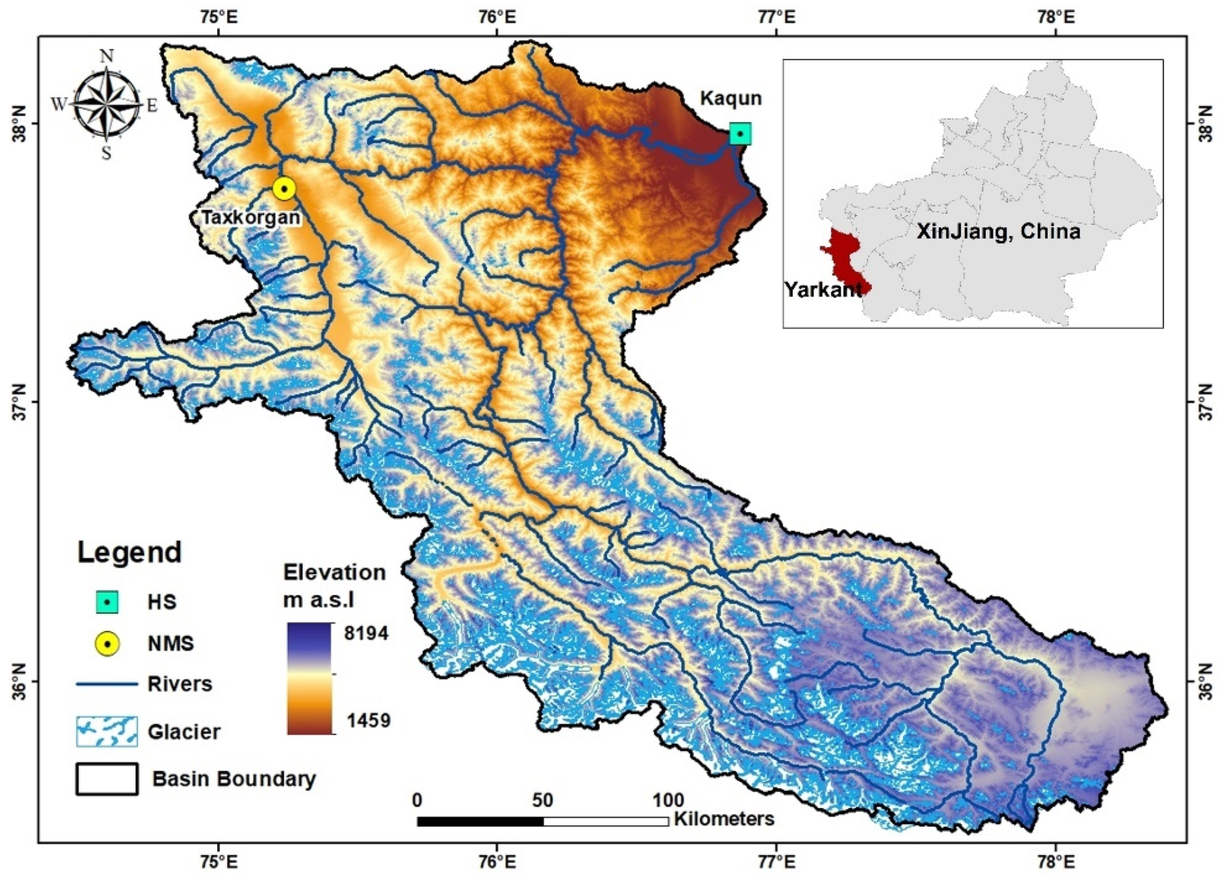
Yarkant River (74°28′–80°54′ E, 34°50′–40°31′ N) is the largest inland river in China and it is one of the heads of the Tarim [52]. Yarkant River basin covers an area of 11.01 × 10⁴ km2, and the basin elevation is about 1459–8194 m [53]. The Yarkant River is mainly supplied by thawed water from the glacier, and the annual thawing volume of the glacier reaches 38.24 × 10⁸ m3. The peak runoff is at August [54,55]. The annual flooding period is from May to September and the dry period is from December to February [56], resulting in the uneven distribution of runoff in a year [57]. The Yarkant River Basin belongs to the temperature continental climate, with an annual precipitation of 47.6 mm and an annual average temperature of 6.2 °C [58].
Yarkant River is located in the hinterland of Asia. It is a typical inland river basin in the arid region [59], and it is extremely sensitive to climate changes. The basin covers a vast territory, great altitude difference, large span, and tough natural conditions [60,61]. In recent years, desertification has been intensifying [62] and soil salinization was very serious (accounting for 38% of the cultivated area) [63]. Agricultural production development has been threatened and restricted significantly [64]. Moreover, the existing water conservancy facilities are very old and insufficient in quantity, thus resulting in a lack of basic data supports and facilities for water resource distribution in the Yarkant River Basin [65,66]. The geographic conditions of Yarkant River are shown in Figure 1.
2.2. Data Sources
In this study, the data of the Yarkant River Basin were collected from the hydrological yearbook of (Kaqun Station) at the Yarkant River (1957–2014). Data included daily temperature, precipitation, and runoff. The time scale was a daily time scale.
The daily temperature, precipitation, and runoff of the Yarkant River Basin from 1957–2014 were collected. A total of 14,000 pieces of data were used in the model test. Time series splicing was performed to all data (temperature, precipitation, and runoff) and then data was converted into csv files. Data samples (top 5 pieces of 14,409) are listed in Table 1.
To reflect interannual variations of meteorological data and runoff in the Yarkant River intuitively, temperature, precipitation, and runoff of the basin were used to plot a broken line/histogram (2002–2014 for example) (Figure 2).
The improved LSTM model has to input temperature, precipitation, and existing runoff data in the basin, and then output the runoff of the prediction year. Before input into the LSTM model, data shall be normalized [67] to meet calculation requirements of the in-depth learning model. The calculation formula of data normalization is:
where is the original value of characteristic data. is the means of characteristic data. is the variance of characteristic data. is the data normalized form (0–1) [68].
After normalization of all characteristics [69], the improved LSTM model converted the time series dataset into a supervised learning problem, to splice attributes at t − 1 and t. The conversion formats are shown in Table 2. The first three columns are river runoff at t − 1, temperature and precipitation at t, respectively, and the fourth column is the runoff at t.
Subsequently, the improved LSTM model separated the above converted dataset (Table 2) into a training set and a test set in the testing process. Data every 6 years was used as the training set, and the data for the next year (7th year) was used as the test set. Later, the training set and test set were decomposed into input and output variables, and then recombined into 3D format ([samples, time steps, and features]), which was expected by LSTM. The machine learning model simulated and predicted the runoff based on this 3D format.
2.3. Methods
2.3.1. LSTM Method
In this study, it was planned to introduce the Long-Short Term Memory (LSTM) model [70]. The LSTM belongs to an in-depth learning algorithm, and its calculation effect is far better than the traditional statistical model. LSTM extracts time series characteristics from the data for modeling. It also collects meteorological characteristics and existing runoffs by analyzing and converting the time series of hydrological data in the river basin [71], thus finishing the simulation and prediction of the river runoff.
LSTM model is an improved form of recurrent neural networks (RNN) [72]. LSTM and RNN have a common point, and they both hypothesize continuous time series as the input samples. However, the middle, with useless information, might make the gradient of RNN disappear when the time series of data is too long. Conversely, the gradient disappearance and explosion, which are caused by the gradient decreasing in the RNN, could be avoided if replacing nodes of the hidden layer of RNN by LSTM and increasing structures such as input gate and output gate. The calculation effect of the LSTM model is superior to the linear model and ordinary neural network.
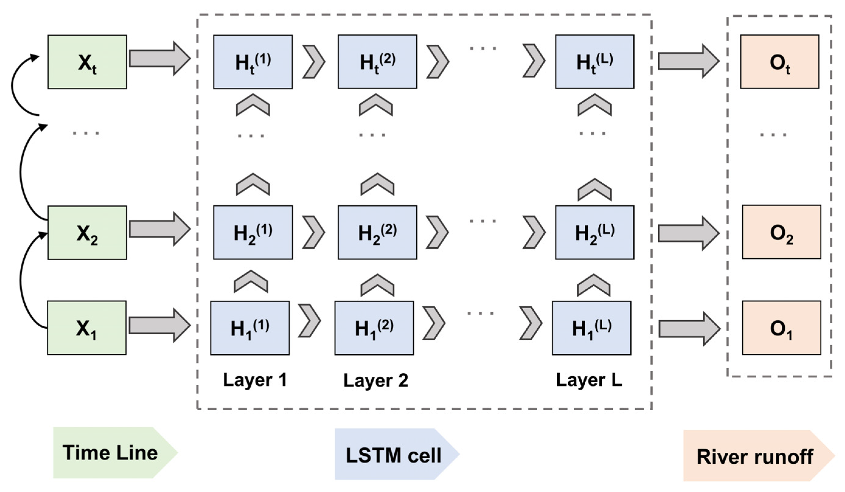
The LSTM model firstly constructs sample data conforming to the LSTM input form (data has been preprocessed and interpreted in Section 2.2) and hyper-parameters were set according to experiences. There were three types of valves of LSTM, including the forget gate, input gate, and output gate. The valve node uses the sigmoid function to calculate the memory state of the network as input [73]. If the output results reached a critical value, the product of this valve output and calculated results of the previous layer were used as the input of the next layer [74]. Otherwise, this output result was forgotten. The weights of each layer, including valve nodes, would be updated on each back propagation training of the model [75]. The principal framework of the improved LSTM model is shown in Figure 3.
The LSTM region has some major characteristics that are different from other neural networks. It can solve the short-term memory problem of RNN, so that the circulation neural network could use long-distance time series information really effectively and speculate the runoff based on meteorological data in a long time series [76].
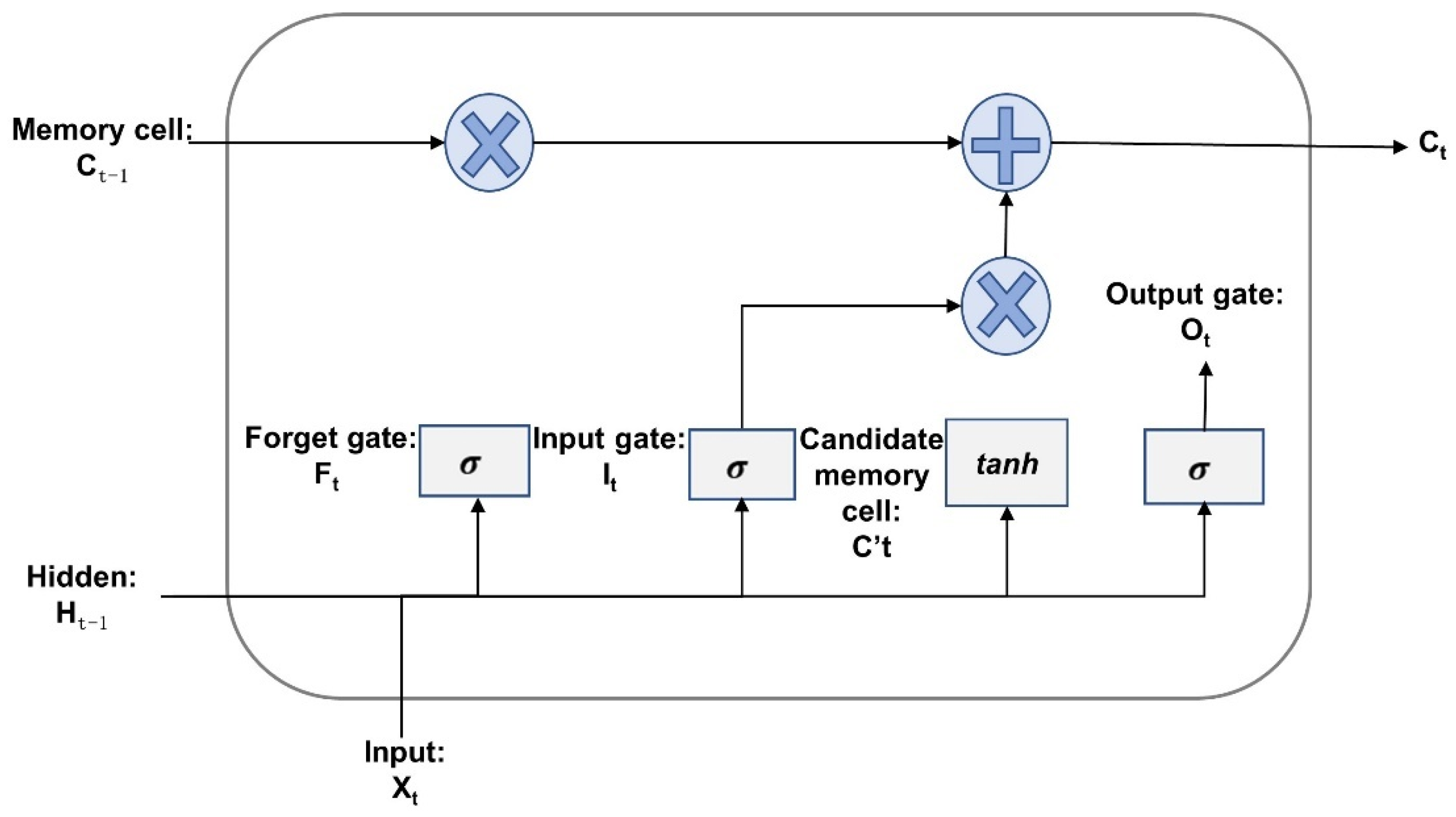
The LSTM model chose a cell as the basic processing unit. To address the structural defects of the traditional RNN, the LSTM added a forget gate, input gate, and output gate in the hidden layer. The forget gate and memory gate were used to select characteristic data, without the use of the pooling operation. Moreover, an information stream, which represented long-term memory, was added, to form a black box with input x and state output o. This was called CELL, which helped LSTM to possess good long-short term memory functions. The CELL structure of LSTM is shown in Figure 4.
Equations (2)–(5) could be combined into:
where is the output at t − 1. is the input at t. is the candidate state at t. refers to the forget gate at t. It controls how much information that the internal state at t − 1 () has to forget. is the input gate, which decides how many network inputs at t () have been stored into the CELL state (). denotes the output gate, which controls how much information of has to be output to the external state .
The transfer function of LSTM CELL was expressed by . When calculating the output of the hidden layer at t, the information stored in CELL at t − 1 was used except for the input vector at t [77]. Therefore, the output of hidden layer under the fixed time step t could be described as
The output of the output layer at t was:
where xi is the input vector at i. is the weight matrix between the hidden layer and output layer, and c is the bias.
LSTM can also cover several network layers, and each network layer had many LSTM CELLs [78]. m refers to the number of LSTM CELLs in the th hidden layer. Therefore, the number of cells in theth hidden layer could be expressed by :
Input of at was the weighted sum of elements in the vector :
The output of at was:
The output of the th hidden layer at was expressed by :
A 5-layer LSTM model was used in this study. The activation function and loss function were Relu and MAE, respectively. The calculation formula of loss was:
where is the predicted value, y is the real value, and n is the number of predictions.
In the training process, the optimization algorithm for parameter updating used Adam, with a learning rate of 0.01. Moreover, training was terminated when finding the optimal result in the verification set.
2.3.2. System Structure
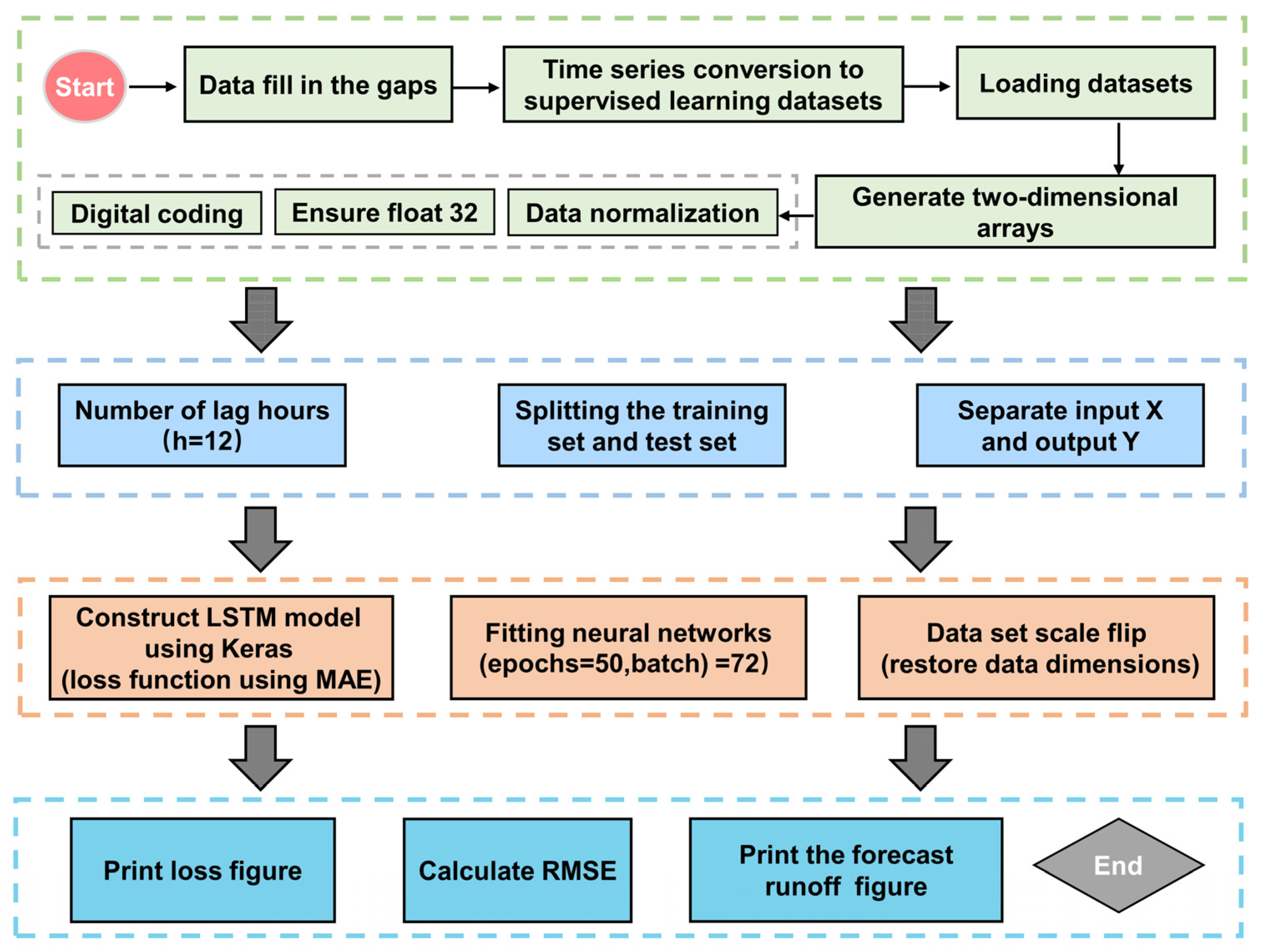
In this study, the LSTM model was introduced for runoff simulation and prediction. The Yarkant River was chosen as the study area. Temperature, precipitation, and existing runoff datasets of the Yarkant River Basin were collected and processed. This dataset involved daily monitoring data in the basin from 1957 to 2014. Such a long-time-series dataset could fully test the long-time-series processing ability of LSTM. The dataset was processed, including filling in gaps, normalization [79], floating-point type conversion, csv format conversion, time series splicing, and sequencing. Moreover, this dataset was divided into a training set and test set to meet the running requirement of the LSTM model.
The processed dataset was input into the LSTM model for runoff prediction. The LSTM model converted time series into a problem of supervised learning, appointed the number of hysteresis hours, and sets the time step to construct the model. After the LSTM model was turned on and obtained the runoff prediction results, a proportional overturn of the calculated results was conducted to reduce the previous normalized numerical values and make them correspond to the real runoff in the basin. The predicted runoff of the model was compared with the existing measured data in the corresponding year. In the comparison, MAE and RMSE were chosen as evaluation indexes [80]. Subsequently, the runoff prediction dataset and accuracy evaluation results (MAE and RMSE) of the LSTM model were output to make prediction results comparable, scientific, and reliable [81].
To present simulation effect intuitively, the comparison diagrams of runoff distributions (including historical runoff of years in the training set, predicted runoff of years in the test set, and real runoff) and the loss function diagram [82] were output in the same time. The running process of LSTM model is shown in Figure 5.
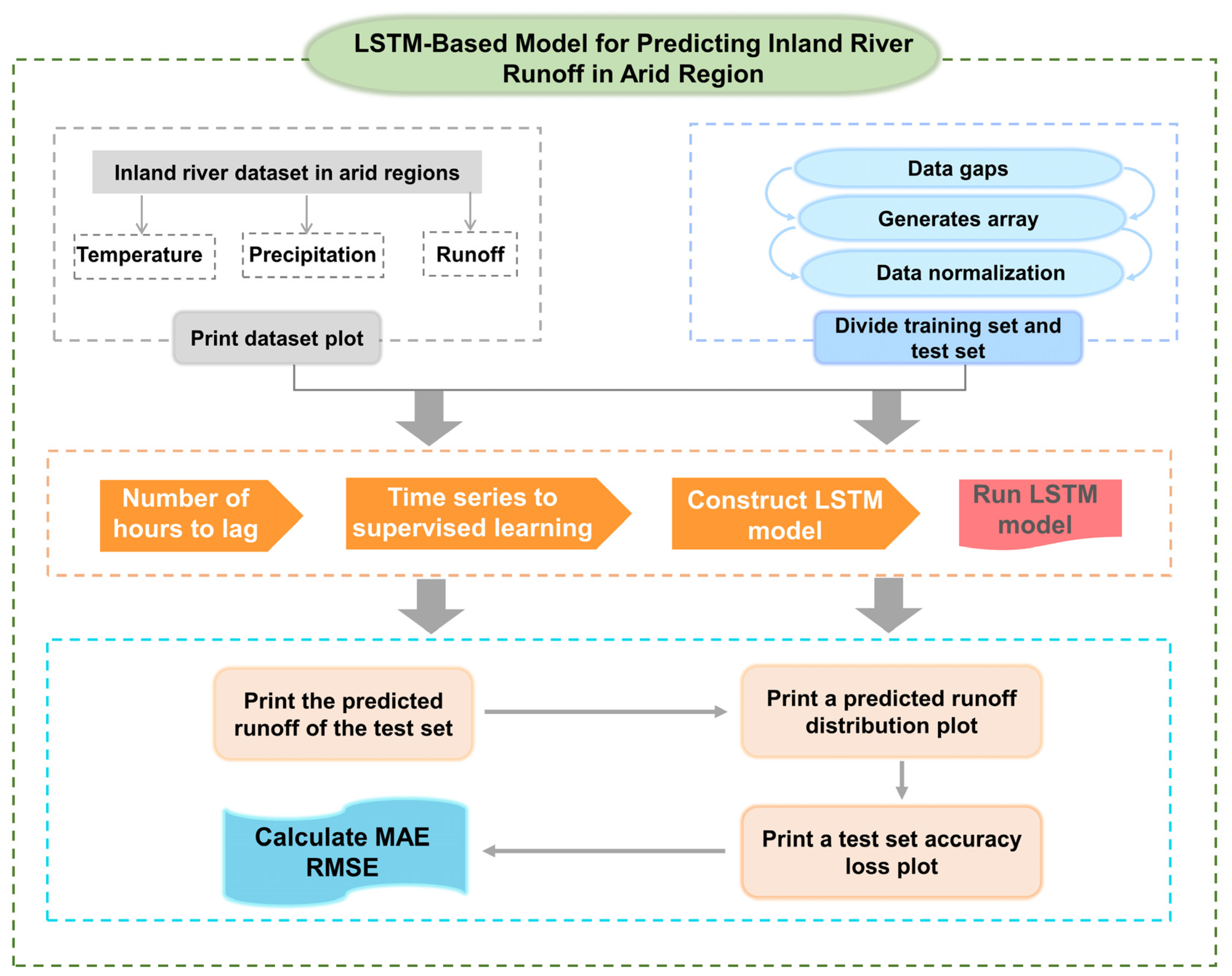
Based on the above principle and running process, the system structure of LSTM model was divided into the data layer, algorithm layer, and user layer [83]. The dataset of the study area was input into the data layer, including daily temperature, precipitation, and existing runoff. All three types of data were merged and normalized. In the algorithm layer, the LSTM model was constructed and evaluated: the dataset was divided into the training set and the test set. The time series dataset was converted into a problem of supervised learning. The LSTM model was constructed and run, and evaluation indexes were appointed (MAE and RMSE). The runoff prediction accuracy of the LSTM model was analyzed and the loss value in the prediction process was output [84]. In this way, the runoff simulation and prediction were finished. The prediction results of runoff and test results of model accuracy were acquired [85]. The user layer could output the runoff prediction value, runoff time-series distribution diagram, accuracy loss diagram, and evaluation results of the LSTM model (MAE and RMSE).
The system structure is shown in Figure 6.
2.4. Evaluation Methods
The LSTM model is superior to other models for the following reasons. It can process long-time series data and store information of preorder input data in the hidden state to improve the understanding of the algorithm on later input data. Therefore, the prediction performances of the LSTM model are improved [86]. To quantize the evaluation results of the LSTM model, MAE and RMSE were chosen as evaluation indexes. Their calculation formulas were:
where predict presents the prediction value of the runoff, real denotes the real value of the runoff, and n refers to the data size.
3. Results
3.1. Comparison with Other Models
To compare performances and accuracy of the LSTM model with other models, four types of prediction models were evaluated, including LSTM, CNN, DTR, and RF. Among them, DTR and RF are statistical models [87], while LSTM and CNN were in-depth learning models. The statistical models have been used in various fields, such as machine learning, medical disease diagnosis, and prediction in the social science field [88]. Nevertheless, they can only predict output probability according to input data [89], but cannot implement statistical classification. CNN and LSTM can provide reliable prediction results and accuracy evaluation through the conversion of input space in the inner layer [90,91]. Therefore, LSTM, CNN, DTR, and RF are applied to simulate and predict runoff data in the Yarkant River. Prediction accuracy of four models was evaluated. MAE and RMSE of the four models are shown in Table 3.
It can be observed from Table 3 that LSTM achieved the optimal prediction effect, with MAE and RMSE of 3.633 and 7.337. The MAE and RMSE of CNN were 8.961 and 12.650, and were slightly better than those of DTR and RF. Prediction effects of DTR and RF were the most unsatisfying. The MAE and RMSE of DTR and RF were relatively similar.
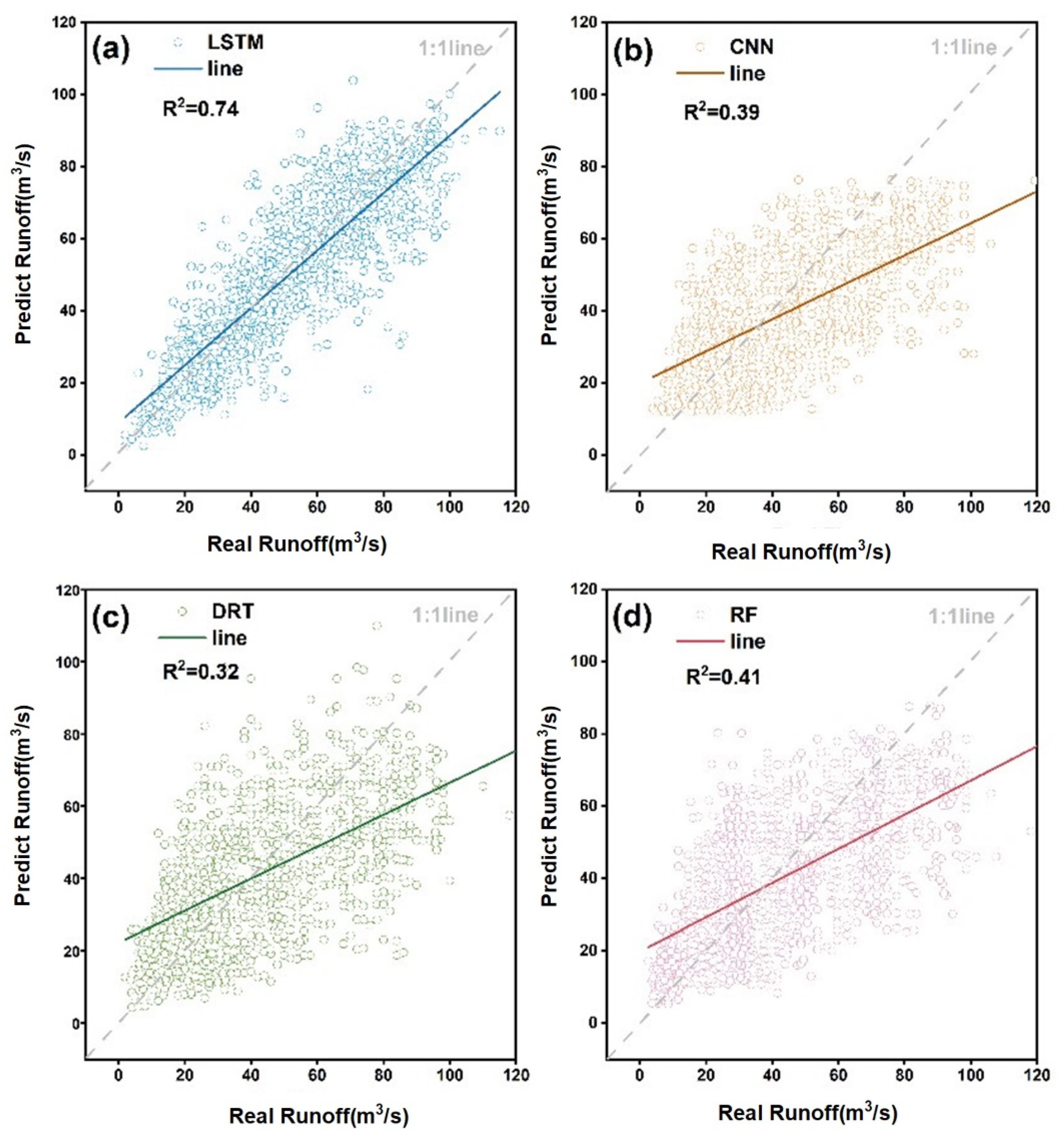
To reflect the prediction effects of four models intuitively, scattering points between prediction values and real values of four models are shown in Figure 7. The results demonstrated that the prediction accuracy of the LSTM model (R2 = 0.74) was significantly higher than those of the rest of the three models.
3.2. LSTM Simulation
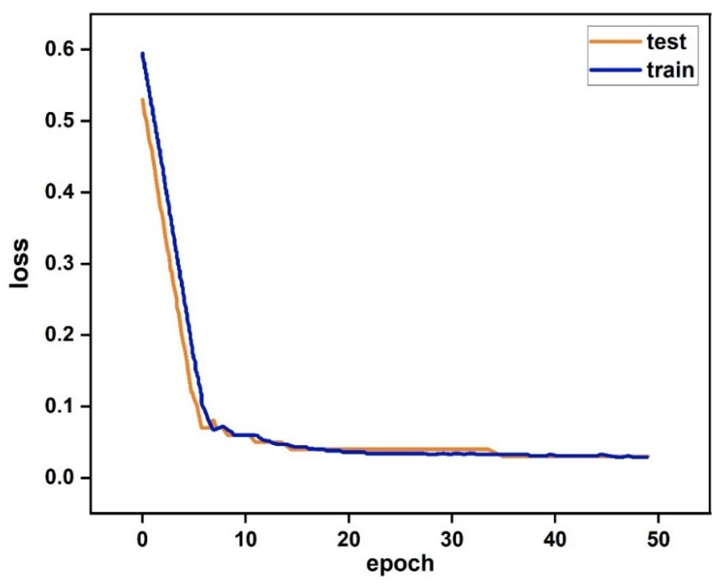
It is inevitable to have accuracy loss and bias during operation of the model. According to the above simulation prediction results of the runoff and the evaluation results of models, the training loss and test loss during the model operation were plotted (Figure 8). The training was divided into 50 epochs and each epoch recorded and plotted losses of the training set and test set. Epoch can be translated as “period” and one epoch refers to the process that all data were inputted into the network to finish one circulation of forward calculation and back propagation. In Figure 8, loss changes in each epoch of the training set and test set were presented. As the epoch increases, the loss gradually stabilizes and approaches a very small value, well below 0.1.
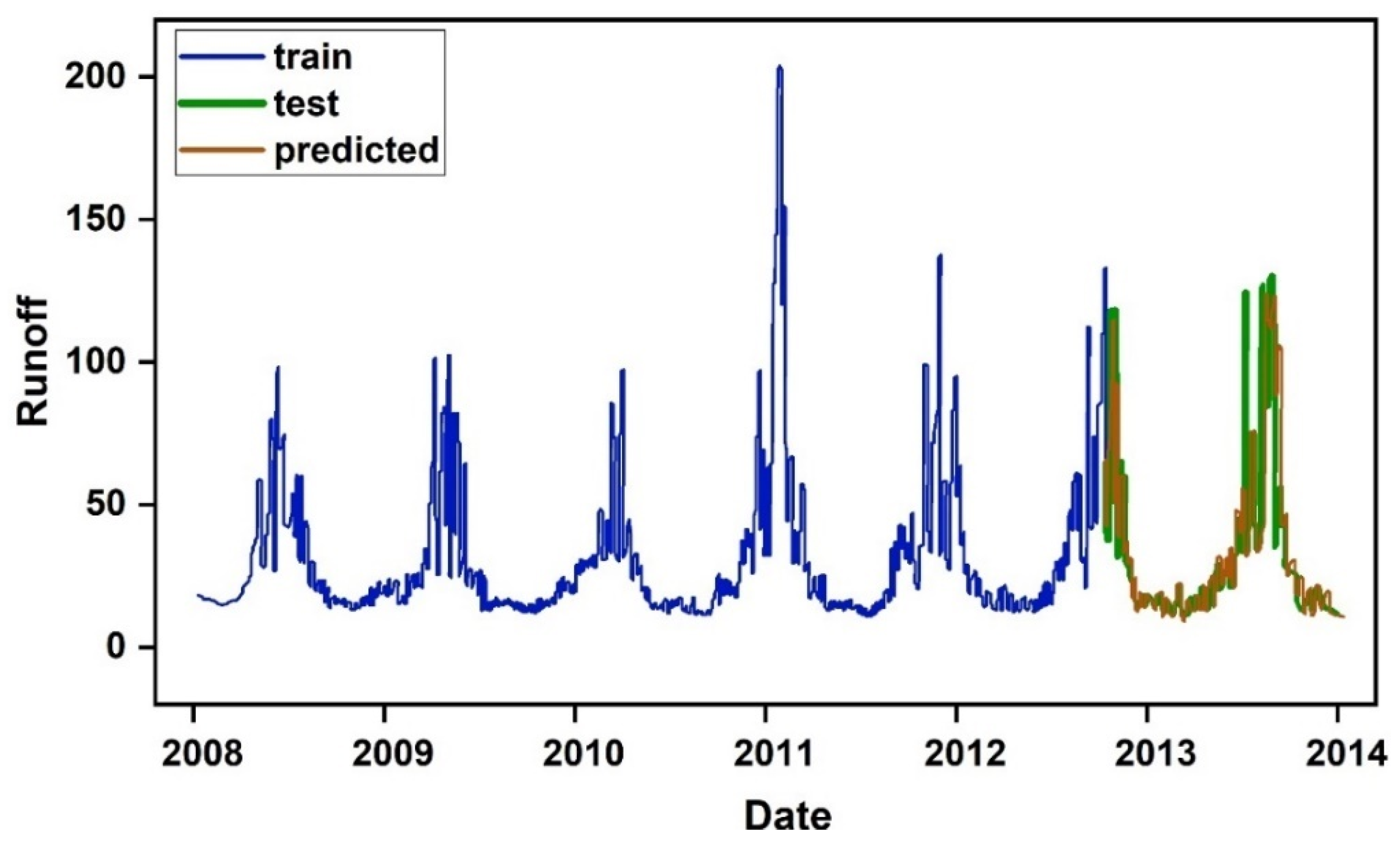
For an intuitive comparison between the prediction value and real value of the runoff, the distribution of prediction results in a period (2008–2014) is shown in Figure 9. Runoff data of the training set and test set were covered. Obviously, the LSTM model presented a better prediction effect of runoff compared to other models. The prediction curve of the LSTM model fit highly with the practical curve.
4. Discussion
It is becoming a research hotspot of hydrology to predict runoff with an in-depth learning algorithm. In 1995, Raman and Sunilkumar [92] applied machine learning to a mid- and long-term (>1 year) runoff forecast. They also constructed a mid- and long-term runoff forecast model based on CNN and used it to forecast runoffs flowing into the Mangalam Reservoir and Pothimdy Reservoir. They verified the advantages of neural network models in the forecast accuracy. Under different time scales, there are some runoff forecast models with good application effects, such as the Regression Model [93,94], Time Series Model [95,96], Gray system model [97,98,99], artificial neural network model (ANN) [100,101], support vector machine model [102,103], machine learning [104,105], etc. These models have different characteristics. They also provide a possibility for a multi-model combined forecast. Based on the rapid development of artificial intelligence and in-depth learning, LSTM is used in hydrological prediction [106] to explore spatial-temporal continuity between the output and relevant input variables [107]. In a study on river runoff in non-arid regions, Fan et al. [108] performed a simulation study on river runoff in the Poyang Lake Basin based on LSTM, and found that the correlation coefficient between the simulation results of the LSTM model and the measured value was higher than 0.9, with an error within ±5%. The LSTM model demonstrated good performances. This was consistent with our research conclusions on the Yarkant River.
Although research on the applications of in-depth learning in the hydrological field have been developing gradually around the world [109], the in-depth learning technology of artificial intelligence is extensively applied in the field for its advantages in feature extraction and simulation optimization [110]. However, in-depth learning is easy to have over-fitting due to the complicated characteristics of the runoff (e.g., unsteady) [111] and inadequate sample size. Therefore, in-depth learning has low simulation accuracy, without good interpretability and scientific references. Although this problem can be relieved by simple data enhancement and regularization, dependence on big data has become a great shortage of in-depth learning. The circulation layer of LSTM can explore series information of the runoff deeply to avoid a long-term dependence problem [112]. It can analyze characteristics of the series data of runoff comprehensively and improve prediction accuracy. In this study, runoff-related meteorological data were coupled, and the time series data was converted into a problem of supervised learning by the LSTM model. This solved difficulties in the calculation and prediction of runoff data, to some extent. Among the existing deep learning methods, LSTM, as a special recurrent neural network, can better handle hydrological data with long-time dependence. Kratzert et al. [47] explored the capability of using LSTM networks for a rainfall-runoff simulation based on experiments conducted on numerous watersheds, which demonstrated that LSTMs have advantages over traditional RNNs in handling long-time series data, concluding that LSTMs should be used instead of traditional RNNs in the runoff simulation based on meteorological data. Kratzert et al. [113] also explored the ability of LSTM models to simulate the runoff in the absence of historical runoff observations for parameter tuning, and demonstrated that generalized models based on LSTM outperformed established basin-specific hydrologic models in most basins. Zhang et al. [114] used the LSTM network for flow prediction of wastewater, and the results demonstrated that the LSTM method has important applications in predicting wastewater flow. The LSTM network can handle time series data well, but there is more redundancy in spatial data processing. Shi et al. [115] proposed a convolutional LSTM network model based on this problem, and successfully applied it to short-time rainfall in instantaneous forecasting. Our next research will also integrate this method and attempt to apply it to inland river basins in arid zones.
With the intensifying global warming [116], the snow thawing period of the glacier is changed and the interannual variation gap of runoff expanded. At the same time, the continuous influence of anthropogenic activities has led to an increasing shortage of water resources in the inland river basins of arid zones [117]. Runoff from arid inland river basins is mostly recharged by ice-snow melt water [118]. Glacier changes caused by climate changes will influence glacier melting [119] and affect the production of snowmelt runoff. This has important influences on the evaluation of total runoff. It can provide important supports to the river runoff prediction in arid regions and improve the accuracy of river runoff estimation models if multi-dimensional meteorological data (glacier melt water) [120] can be coupled except for meteorological data. Furthermore, algorithms that set weights of influencing factors, such as the attention learning algorithm, can be added into the LSTM model [121] to realize a multi-parameter change of influencing factors and combine multiple in-depth learning models. This can meet natural environmental conditions of rivers under different scenarios, and increase the applicability of runoff prediction models. The results can provide references to ecological restoration and water resource distribution in arid regions.
5. Conclusions
This study simulates and estimates inland river runoff in arid regions by introducing the in-depth learning algorithm of LSTM. A case study based on the Yarkant River Basin is performed. LSTM converts time series data into a problem of supervised learning by coupling runoff-related meteorological factors (daily temperature, precipitation, and existing runoff of the study area). It simulates and predicts runoff in the Yarkant River, and solves the long-time series data over-fitting of the neural network. Moreover, accuracy of the LSTM model is evaluated by MAE and RMSE. Meanwhile, experimental results of four models (LSTM, CNN, RF, and DRT) are compared. The results demonstrate that the prediction effect of LSTM model is significantly better than those of CNN, DTR, and RF, with MAE and RMSE of 3.633 and 7.337. The improved runoff simulation and prediction model based on LSTM also applies to the runoff simulation and prediction of other inland rivers in arid regions. On one hand, they can provide theoretical references and technological supports to reasonable development, utilization, and management of water resources in the Yarkant River Basin. On the other hand, they can provide references to the runoff prediction of inland rivers in arid regions. This study is of important significance to improve the effective utilization and allocation of water resources in arid regions.
Author Contributions
Conceptualization, J.L. and X.M.; methodology, J.L., X.M., and W.Y.; software, J.L. and K.Q.; validation, X.Y. and X.M.; formal analysis, J.L. and Y.L.; data curation, J.L.; writing—original draft preparation, J.L. and X.M.; writing—review and editing, J.L. and X.M; supervision, G.L. and X.M. All authors have read and agreed to the published version of the manuscript.
Funding
This research was funded by the National Natural Science Foundation of China (42101302), China Postdoctoral Science Foundation (2021M703470), and the Strategic Priority Research Program of the Chinese Academy of Sciences (XDA2006030201) for their sponsorship.
Institutional Review Board Statement
Not applicable.
Informed Consent Statement
Not applicable.
Data Availability Statement
Not applicable.
Acknowledgments
We would like to express our sincere thanks to the anonymous reviewers.
Conflicts of Interest
The authors declare no conflict of interest.
References
- Al-Fugara, A.K.; Ahmadlou, M.; Shatnawi, R.; AlAyyash, S.; Al-Adamat, R.; Al-Shabeeb, A.A.-R.; Soni, S. Novel hybrid models combining meta-heuristic algorithms with support vector regression (SVR) for groundwater potential mapping. Geocarto Int. 2020, 1–20. [Google Scholar] [CrossRef]
- Wang, H.; Chen, Y.; Pan, Y.; Li, W. Spatial and temporal variability of drought in the arid region of China and its relationships to teleconnection indices. J. Hydrol. 2015, 523, 283–296. [Google Scholar] [CrossRef]
- Ryu, Y.; Jiang, C.; Kobayashi, H.; Detto, M. MODIS-derived global land products of shortwave radiation and diffuse and total photosynthetically active radiation at 5 km resolution from 2000. Remote Sens. Environ. 2018, 204, 812–825. [Google Scholar] [CrossRef]
- Yang, Y.; Bai, L.; Wang, B.; Wu, J.; Fu, S. Reliability of the global climate models during 1961–1999 in arid and semiarid regions of China. Sci. Total Environ. 2019, 667, 271–286. [Google Scholar] [CrossRef] [PubMed]
- Gaur, M.K.; Squires, V.R. Geographic extent and characteristics of the world’s arid zones and their peoples. In Climate Variability Impacts on Land Use and Livelihoods in Drylands; Springer: Berlin/Heidelberg, Germany, 2018; pp. 3–20. [Google Scholar]
- Hatibu, N. Rainwater Management: Strategies for Improving Water Availability and Productivity in Semi-Arid and Arid Areas; International Water Management Institute: Anand, India, 2002. [Google Scholar]
- Giles, D.M.; Sinyuk, A.; Sorokin, M.G.; Schafer, J.S.; Smirnov, A.; Slutsker, I.; Eck, T.F.; Holben, B.N.; Lewis, J.R.; Campbell, J.R.; et al. Advancements in the Aerosol Robotic Network (AERONET) Version 3 database—Automated near-real-time quality control algorithm with improved cloud screening for Sun photometer aerosol optical depth (AOD) measurements. Atmos. Meas. Tech. 2019, 12, 169–209. [Google Scholar] [CrossRef] [Green Version]
- Lu, N.; Wang, M.; Ning, B.; Yu, D.; Fu, B. Research advances in ecosystem services in drylands under global environmental changes. Curr. Opin. Environ. Sustain. 2018, 33, 92–98. [Google Scholar] [CrossRef]
- Magalhaes, A.R. Sustainable development planning and semi-arid regions. Glob. Environ. Change 1994, 4, 275–279. [Google Scholar] [CrossRef]
- Lourenço, N.; Russo Machado, C. Water Resources and Sustainable Development: Factors and Constraints for Improving Human Well-Being in Water-Stressed Regions; School of the Environment of Nanjing University: Nanjing, China, 2005. [Google Scholar]
- Liu, Y.; Du, J.; Ding, B.; Liu, Y.; Liu, W.; Xia, A.; Huo, R.; Ran, Q.; Hao, Y.; Cui, X. Water resource conservation promotes synergy between economy and environment in China’s northern drylands. Front. Environ. Sci. Eng. 2022, 16, 1–12. [Google Scholar] [CrossRef]
- Stringer, L.C.; Mirzabaev, A.; Benjaminsen, T.A.; Harris, R.M.; Jafari, M.; Lissner, T.K.; Stevens, N.; Tirado-von Der Pahlen, C. Climate change impacts on water security in global drylands. One Earth 2021, 4, 851–864. [Google Scholar] [CrossRef]
- Ma, J.; Wang, X.; Edmunds, W. The characteristics of ground-water resources and their changes under the impacts of human activity in the arid Northwest China—A case study of the Shiyang River Basin. J. Arid Environ. 2005, 61, 277–295. [Google Scholar] [CrossRef]
- Rockström, J.; Falkenmark, M.; Allan, T.; Folke, C.; Gordon, L.; Jägerskog, A.; Kummu, M.; Lannerstad, M.; Meybeck, M.; Molden, D. The unfolding water drama in the Anthropocene: Towards a resilience-based perspective on water for global sustainability. Ecohydrology 2014, 7, 1249–1261. [Google Scholar] [CrossRef]
- Cassardo, C.; Jones, J.A.A. Managing Water in a Changing World; Molecular Diversity Preservation International: Basel, Switzerland, 2011; Volume 3, pp. 618–628. [Google Scholar]
- Van Dijk, A.I.; Beck, H.E.; Crosbie, R.S.; de Jeu, R.A.; Liu, Y.Y.; Podger, G.M.; Timbal, B.; Viney, N.R. The Millennium Drought in southeast Australia (2001–2009): Natural and human causes and implications for water resources, ecosystems, economy, and society. Water Resour. Res. 2013, 49, 1040–1057. [Google Scholar] [CrossRef]
- Jury, W.A.; Vaux, H.J., Jr. The emerging global water crisis: Managing scarcity and conflict between water users. Adv. Agron. 2007, 95, 1–76. [Google Scholar]
- Richter, B.D.; Mathews, R.; Harrison, D.L.; Wigington, R. Ecologically sustainable water management: Managing river flows for ecological integrity. Ecol. Appl. 2003, 13, 206–224. [Google Scholar] [CrossRef]
- Wu, G.; Li, L.; Ahmad, S.; Chen, X.; Pan, X. A dynamic model for vulnerability assessment of regional water resources in arid areas: A case study of Bayingolin, China. Water Resour. Manag. 2013, 27, 3085–3101. [Google Scholar] [CrossRef]
- Grundmann, J.; Schütze, N.; Schmitz, G.H.; Al-Shaqsi, S. Towards an integrated arid zone water management using simulation-based optimisation. Environ. Earth Sci. 2012, 65, 1381–1394. [Google Scholar] [CrossRef]
- Ragab, R.; Prudhomme, C. Sw—soil and Water: Climate change and water resources management in arid and semi-arid regions: Prospective and challenges for the 21st century. Biosyst. Eng. 2002, 81, 3–34. [Google Scholar]
- Chen, Y.; Li, Z.; Fan, Y.; Wang, H.; Deng, H. Progress and prospects of climate change impacts on hydrology in the arid region of northwest China. Environ. Res. 2015, 139, 11–19. [Google Scholar] [CrossRef]
- Pilgrim, D.; Chapman, T.; Doran, D. Problems of rainfall-runoff modelling in arid and semiarid regions. Hydrol. Sci. J. 1988, 33, 379–400. [Google Scholar] [CrossRef]
- Derdour, A.; Bouanani, A.; Babahamed, K. Modelling rainfall runoff relations using HEC-HMS in a semi-arid region: Case study in Ain Sefra watershed, Ksour Mountains (SW Algeria). J. Water Land Dev. 2018, 36, 45–55. [Google Scholar] [CrossRef] [Green Version]
- Muneer, A.S.; Sayl, K.N.; Kamel, A.H. Modeling of runoff in the arid regions using remote sensing and geographic information system (GIS). Int. J. Des. Nat. Ecodynamics 2020, 15, 691–700. [Google Scholar] [CrossRef]
- Chen, Y.; Li, B.; Li, Z.; Li, W. Water resource formation and conversion and water security in arid region of Northwest China. J. Geogr. Sci. 2016, 26, 939–952. [Google Scholar] [CrossRef] [Green Version]
- Silva, T.A.; Ferreira, J.; Calijuri, M.L.; dos Santos, V.J.; do Carmo Alves, S.; de Siqueira Castro, J. Efficiency of technologies to live with drought in agricultural development in Brazil’s semi-arid regions. J. Arid Environ. 2021, 192, 104538. [Google Scholar] [CrossRef]
- Yang, T.; Wang, S.; Li, X.; Wu, T.; Li, L.; Chen, J. River habitat assessment for ecological restoration of Wei River Basin, China. Environ. Sci. Pollut. Res. 2018, 25, 17077–17090. [Google Scholar] [CrossRef]
- Wu, W.; Xu, Z.; Zhan, C.; Yin, X.; Yu, S. A new framework to evaluate ecosystem health: A case study in the Wei River basin, China. Environ. Monit. Assess. 2015, 187, 1–15. [Google Scholar] [CrossRef]
- Saadati, H.; Gholami, S.A.; Sharifi, F.; AYOUBZADEH, S.A. An investigation of the effects of land use change on simulating surface runoff using SWAT mathematical model (case study: Kasilian catchment area). Iran. J. Nat. Resour. 2006, 59, 301–313. [Google Scholar]
- Singh, V.P.; Woolhiser, D.A. Mathematical modeling of watershed hydrology. J. Hydrol. Eng. 2002, 7, 270–292. [Google Scholar] [CrossRef] [Green Version]
- Shende, S. A conceptual rainfall-runoff mathematical model to simulate runoff using daily amount of rainfall for arid and semi-arid region. In Proceedings of Journal of Physics: Conference Series; IOP Publishing: Bristol, UK, 2021; p. 022017. [Google Scholar]
- Abdessamed, D.; Abderrazak, B. Coupling HEC-RAS and HEC-HMS in rainfall–runoff modeling and evaluating floodplain inundation maps in arid environments: Case study of Ain Sefra city, Ksour Mountain. SW of Algeria. Environ. Earth Sci. 2019, 78, 586. [Google Scholar] [CrossRef]
- Lange, H.; Sippel, S. Machine learning applications in hydrology. In Forest-Water Interactions; Springer: Berlin/Heidelberg, Germany, 2020; pp. 233–257. [Google Scholar]
- Gimblett, H.R. Integrating geographic information systems and agent-based technologies for modeling and simulating social and ecological phenomena. In Integrating Geographic Information Systems and Agent-Based Modeling Techniques for Understanding Social and Ecological Processes; Oxford University Press: Oxford, UK, 2002. [Google Scholar]
- Hosseini, F.S.; Choubin, B.; Mosavi, A.; Nabipour, N.; Shamshirband, S.; Darabi, H.; Haghighi, A.T. Flash-flood hazard assessment using ensembles and Bayesian-based machine learning models: Application of the simulated annealing feature selection method. Sci. Total Environ. 2020, 711, 135161. [Google Scholar] [CrossRef]
- Tanty, R.; Desmukh, T.S. Application of artificial neural network in hydrology—A review. Int. J. Eng. Technol. Res. 2015, 4, 184–188. [Google Scholar]
- Solomatine, D.P.; Ostfeld, A. Data-driven modelling: Some past experiences and new approaches. J. Hydroinform. 2008, 10, 3–22. [Google Scholar] [CrossRef] [Green Version]
- Fa, W.; Wieczorek, M.A.; Heggy, E. Modeling polarimetric radar scattering from the lunar surface: Study on the effect of physical properties of the regolith layer. J. Geophys. Res. Planets 2011, 116. [Google Scholar] [CrossRef]
- Fatichi, S.; Vivoni, E.R.; Ogden, F.L.; Ivanov, V.Y.; Mirus, B.; Gochis, D.; Downer, C.W.; Camporese, M.; Davison, J.H.; Ebel, B. An overview of current applications, challenges, and future trends in distributed process-based models in hydrology. J. Hydrol. 2016, 537, 45–60. [Google Scholar] [CrossRef] [Green Version]
- Agarwal, A.; Singh, R. Runoff modelling through back propagation artificial neural network with variable rainfall-runoff data. Water Resour. Manag. 2004, 18, 285–300. [Google Scholar] [CrossRef]
- Boulmaiz, T.; Ouerdachi, L.; Boutoutaou, D.; Boutaghane, H. Single neural network and neuro-updating conceptual model for forecasting runoff. Int. J. Hydrol. Sci. Technol. 2016, 6, 344–358. [Google Scholar] [CrossRef]
- Van, S.P.; Le, H.M.; Thanh, D.V.; Dang, T.D.; Loc, H.H.; Anh, D.T. Deep learning convolutional neural network in rainfall–runoff modelling. J. Hydroinform. 2020, 22, 541–561. [Google Scholar] [CrossRef]
- Hu, C.; Wu, Q.; Li, H.; Jian, S.; Li, N.; Lou, Z. Deep learning with a long short-term memory networks approach for rainfall-runoff simulation. Water 2018, 10, 1543. [Google Scholar] [CrossRef] [Green Version]
- Gers, F.A.; Schraudolph, N.N.; Schmidhuber, J. Learning precise timing with LSTM recurrent networks. J. Mach. Learn. Res. 2002, 3, 115–143. [Google Scholar]
- Yu, Y.; Si, X.; Hu, C.; Zhang, J. A review of recurrent neural networks: LSTM cells and network architectures. Neural Comput. 2019, 31, 1235–1270. [Google Scholar] [CrossRef]
- Kratzert, F.; Klotz, D.; Brenner, C.; Schulz, K.; Herrnegger, M. Rainfall–runoff modelling using long short-term memory (LSTM) networks. Hydrol. Earth Syst. Sci. 2018, 22, 6005–6022. [Google Scholar] [CrossRef] [Green Version]
- Xiang, Z.; Yan, J.; Demir, I. A rainfall-runoff model with LSTM-based sequence-to-sequence learning. Water Resour. Res. 2020, 56, e2019WR025326. [Google Scholar] [CrossRef]
- Wang, J.; Li, H.; Hao, X. Responses of snowmelt runoff to climatic change in an inland river basin, Northwestern China, over the past 50 years. Hydrol. Earth Syst. Sci. 2010, 14, 1979–1987. [Google Scholar] [CrossRef] [Green Version]
- Zhang, Q.; Xu, C.-Y.; Tao, H.; Jiang, T.; Chen, Y.D. Climate changes and their impacts on water resources in the arid regions: A case study of the Tarim River basin, China. Stoch. Environ. Res. Risk Assess. 2010, 24, 349–358. [Google Scholar] [CrossRef]
- Butterworth, J.; Warner, J.; Moriarty, P.; Smits, S.; Batchelor, C. Finding practical approaches to integrated water resources management. Water Altern. 2010, 3, 68–81. [Google Scholar]
- Wei, R.-j.; Peng, L.; Liang, C.; Haemmig, C.; Huss, M.; Mu, Z.-x.; He, Y. Analysis of temporal and spatial variations in hydrometeorological elements in the Yarkant River Basin, China. J. Water Clim. Change 2019, 10, 167–180. [Google Scholar] [CrossRef] [Green Version]
- Ma, X.; Yan, W.; Zhao, C.; Kundzewicz, Z.W. Snow-cover area and runoff variation under climate change in the West Kunlun Mountains. Water-Sui 2019, 11, 2246. [Google Scholar] [CrossRef] [Green Version]
- Chen, Y.; Xu, C.; Chen, Y.; Li, W.; Liu, J. Response of glacial-lake outburst floods to climate change in the Yarkant River basin on northern slope of Karakoram Mountains, China. Quat. Int. 2010, 226, 75–81. [Google Scholar] [CrossRef]
- Yaning, C.; Changchun, X.; Xingming, H.; Weihong, L.; Yapeng, C.; Chenggang, Z.; Zhaoxia, Y. Fifty-year climate change and its effect on annual runoff in the Tarim River Basin, China. Quat. Int. 2009, 208, 53–61. [Google Scholar]
- Fan, Y.; Chen, Y.; Liu, Y.; Li, W. Variation of baseflows in the headstreams of the Tarim River Basin during 1960–2007. J. Hydrol. 2013, 487, 98–108. [Google Scholar] [CrossRef]
- Chen, Y.-n.; Li, W.-h.; Xu, C.-c.; Hao, X.-m. Effects of climate change on water resources in Tarim River Basin, Northwest China. J. Environ. Sci. 2007, 19, 488–493. [Google Scholar] [CrossRef]
- Xiang, Y.; Wang, Y.; Chen, Y.; Zhang, Q. Impact of Climate Change on the Hydrological Regime of the Yarkant River Basin, China: An Assessment Using Three SSP Scenarios of CMIP6 GCMs. Remote Sens. 2021, 14, 115. [Google Scholar] [CrossRef]
- Kan, B.; Su, F.; Xu, B.; Xie, Y.; Li, J.; Zhang, H. Generation of high mountain precipitation and temperature data for a quantitative assessment of flow regime in the Upper Yarkant basin in the Karakoram. J. Geophys. Res. Atmos. 2018, 123, 8462–8486. [Google Scholar] [CrossRef]
- Fan, Z.; Xia, X.; Shen, Y.; Alishir, K.; Wang, R.; Li, S.; Ma, Y. Utilization of water resources, ecological balance and land desertification in the Tarim Basin, Xinjiang. Sci. China Ser. D Earth Sci. 2002, 45, 102–108. [Google Scholar] [CrossRef]
- Bruelheide, H.; Jandt, U.; Gries, D.; Thomas, F.M.; Foetzki, A.; Bürkert, A.; Wang, G.; Zhang, X.; Runge, M. Vegetation Changes in a River Oasis on the Southern Rim of the Taklamakan Desert in China between 1956 and 2000; Borntraeger: Stuttgart, Germany, 2003. [Google Scholar]
- Li, D.; Xu, E.; Zhang, H. Influence of ecological land change on wind erosion prevention service in arid area of northwest China from 1990 to 2015. Ecol. Indic. 2020, 117, 106686. [Google Scholar] [CrossRef]
- Wang, B.; Dong, X.; Wang, Z.; Qin, G. Characterizing spatiotemporal variations of soil salinization and its relationship with eco-hydrological parameters at the Regional Scale in the Kashi Area of Xinjiang, China from 2000 to 2017. Water 2021, 13, 1075. [Google Scholar] [CrossRef]
- Liu, Y.; Tian, F.; Hu, H.; Sivapalan, M. Socio-hydrologic perspectives of the co-evolution of humans and water in the Tarim River basin, Western China: The Taiji–Tire model. Hydrol. Earth Syst. Sci. 2014, 18, 1289–1303. [Google Scholar] [CrossRef] [Green Version]
- Shen, Y.; Li, S.; Chen, Y.; Qi, Y.; Zhang, S. Estimation of regional irrigation water requirement and water supply risk in the arid region of Northwestern China 1989–2010. Agric. Water Manag. 2013, 128, 55–64. [Google Scholar] [CrossRef]
- Yang, F.; Xue, L.; Wei, G.; Chi, Y.; Yang, G. Study on the dominant causes of streamflow alteration and effects of the current water diversion in the Tarim River Basin, China. Hydrol. Processes 2018, 32, 3391–3401. [Google Scholar] [CrossRef]
- Abdulrazzaq, Z.T.; Hasan, R.H.; Aziz, N.A. Integrated TRMM data and standardized precipitation index to monitor the meteorological drought. Civ. Eng. J. 2019, 5, 1590–1598. [Google Scholar] [CrossRef] [Green Version]
- Legates, D.R.; Willmott, C.J. Mean seasonal and spatial variability in global surface air temperature. Theor. Appl. Climatol. 1990, 41, 11–21. [Google Scholar] [CrossRef]
- Suarez-Alvarez, M.M.; Pham, D.-T.; Prostov, M.Y.; Prostov, Y.I. Statistical approach to normalization of feature vectors and clustering of mixed datasets. Proc. R. Soc. A Math. Phys. Eng. Sci. 2012, 468, 2630–2651. [Google Scholar] [CrossRef]
- Liu, M.; Huang, Y.; Li, Z.; Tong, B.; Liu, Z.; Sun, M.; Jiang, F.; Zhang, H. The applicability of LSTM-KNN model for real-time flood forecasting in different climate zones in China. Water 2020, 12, 440. [Google Scholar] [CrossRef] [Green Version]
- Papacharalampous, G.; Tyralis, H.; Papalexiou, S.M.; Langousis, A.; Khatami, S.; Volpi, E.; Grimaldi, S. Global-scale massive feature extraction from monthly hydroclimatic time series: Statistical characterizations, spatial patterns and hydrological similarity. Sci. Total Environ. 2021, 767, 144612. [Google Scholar] [CrossRef] [PubMed]
- Bai, Y.; Bezak, N.; Zeng, B.; Li, C.; Sapač, K.; Zhang, J. Daily runoff forecasting using a cascade long short-term memory model that considers different variables. Water Resour. Manag. 2021, 35, 1167–1181. [Google Scholar]
- Ni, L.; Wang, D.; Singh, V.P.; Wu, J.; Wang, Y.; Tao, Y.; Zhang, J. Streamflow and rainfall forecasting by two long short-term memory-based models. J. Hydrol. 2020, 583, 124296. [Google Scholar] [CrossRef]
- Li, F.; Ma, G.; Chen, S.; Huang, W. An Ensemble Modeling Approach to Forecast Daily Reservoir Inflow Using Bidirectional Long-and Short-Term Memory (Bi-LSTM), Variational Mode Decomposition (VMD), and Energy Entropy Method. Water Resour. Manag. 2021, 35, 2941–2963. [Google Scholar] [CrossRef]
- Jing, X.; Luo, J.; Zhang, S.; Wei, N. Runoff forecasting model based on variational mode decomposition and artificial neural networks. Math. Biosci. Eng. 2022, 19, 1633–1648. [Google Scholar] [CrossRef]
- Kratzert, F.; Klotz, D.; Shalev, G.; Klambauer, G.; Hochreiter, S.; Nearing, G. Benchmarking a catchment-aware long short-term memory network (LSTM) for large-scale hydrological modeling. Hydrol. Earth Syst. Sci. Discuss. 2019, 1–32. [Google Scholar]
- Chen, Y.-C.; Gao, J.-J.; Bin, Z.-H.; Qian, J.-Z.; Pei, R.-L.; Zhu, H. Application study of IFAS and LSTM models on runoff simulation and flood prediction in the Tokachi River basin. J. Hydroinform. 2021, 23, 1098–1111. [Google Scholar] [CrossRef]
- Tao, S.; Fang, J.; Ma, S.; Cai, Q.; Xiong, X.; Tian, D.; Zhao, X.; Fang, L.; Zhang, H.; Zhu, J.J.N.S.R. Changes in China’s lakes: Climate and human impacts. Natl. Sci. Rev. 2020, 7, 132–140. [Google Scholar] [CrossRef] [Green Version]
- Yozgatligil, C.; Aslan, S.; Iyigun, C.; Batmaz, I. Comparison of missing value imputation methods in time series: The case of Turkish meteorological data. Theor. Appl. Climatol. 2013, 112, 143–167. [Google Scholar] [CrossRef]
- Wang, W.; Lu, Y. Analysis of the mean absolute error (MAE) and the root mean square error (RMSE) in assessing rounding model. In Proceedings of IOP Conference Series: Materials Science and Engineering; IOP Publishing: Bristol, UK, 2020; p. 012049. [Google Scholar]
- Gauch, M.; Kratzert, F.; Klotz, D.; Nearing, G.; Lin, J.; Hochreiter, S. Rainfall–runoff prediction at multiple timescales with a single Long Short-Term Memory network. Hydrol. Earth Syst. Sci. 2021, 25, 2045–2062. [Google Scholar] [CrossRef]
- Han, H.; Morrison, R.R. Data-driven approaches for runoff prediction using distributed data. Stoch. Environ. Res. Risk Assess. 2021, 1–19. [Google Scholar] [CrossRef]
- Nasser, A.A.; Rashad, M.Z.; Hussein, S.E. A two-layer water demand prediction system in urban areas based on micro-services and LSTM neural networks. IEEE Access 2020, 8, 147647–147661. [Google Scholar] [CrossRef]
- Quan, Q.; Hao, Z.; Xifeng, H.; Jingchun, L. Research on water temperature prediction based on improved support vector regression. Neural Comput. Appl. 2020, 34, 8501–8510. [Google Scholar] [CrossRef]
- Zhao, Z.; Chen, W.; Wu, X.; Chen, P.C.; Liu, J. LSTM network: A deep learning approach for short-term traffic forecast. IET Intell. Transp. Syst. 2017, 11, 68–75. [Google Scholar] [CrossRef] [Green Version]
- Xu, Y.; Liu, Y.; Jiang, Z.; Yang, X. Runoff Prediction Model Based on Improved Convolutional Neural Network. Water Resour. Manag. 2021. Reprint. [Google Scholar] [CrossRef]
- Contreras, P.; Orellana-Alvear, J.; Muñoz, P.; Bendix, J.; Célleri, R. Influence of random forest hyperparameterization on short-term runoff forecasting in an andean mountain catchment. Atmosphere 2021, 12, 238. [Google Scholar] [CrossRef]
- Oppel, H.; Schumann, A.H. Machine learning based identification of dominant controls on runoff dynamics. Hydrol. Processes 2020, 34, 2450–2465. [Google Scholar] [CrossRef]
- Müftüoğlu, R.F. Monthly runoff generation by non-linear models. J. Hydrol. 1991, 125, 277–291. [Google Scholar] [CrossRef]
- Chen, S.; Dong, S.; Cao, Z.; Guo, J. A compound approach for monthly runoff forecasting based on multiscale analysis and deep network with sequential structure. Water 2020, 12, 2274. [Google Scholar] [CrossRef]
- Li, P.; Zhang, J.; Krebs, P. Prediction of Flow Based on a CNN-LSTM Combined Deep Learning Approach. Water 2022, 14, 993. [Google Scholar] [CrossRef]
- Raman, H.; Sunilkumar, N. Multivariate modelling of water resources time series using artificial neural networks. Hydrol. Sci. J. 1995, 40, 145–163. [Google Scholar] [CrossRef]
- Nawaz, N.; Adeloye, A. Evaluation of monthly runoff estimated by a rainfall-runoff regression model for reservoir yield assessment. Hydrol. Sci. J. 1999, 44, 113–134. [Google Scholar] [CrossRef] [Green Version]
- Özelkan, E.C.; Duckstein, L. Fuzzy conceptual rainfall–runoff models. J. Hydrol. 2001, 253, 41–68. [Google Scholar] [CrossRef]
- Willems, P. A time series tool to support the multi-criteria performance evaluation of rainfall-runoff models. Environ. Model. Softw. 2009, 24, 311–321. [Google Scholar] [CrossRef]
- Wang, W.-C.; Chau, K.-W.; Xu, D.-M.; Chen, X.-Y. Improving forecasting accuracy of annual runoff time series using ARIMA based on EEMD decomposition. Water Resour. Manag. 2015, 29, 2655–2675. [Google Scholar] [CrossRef]
- Trivedi, H.; Singh, J. Application of grey system theory in the development of a runoff prediction model. Biosyst. Eng. 2005, 92, 521–526. [Google Scholar] [CrossRef]
- Yu, P.S.; Chen, C.J.; Chen, S.J.; Lin, S.C. Application of Grey Model toward Runoff Forecasting 1. JAWRA J. Am. Water Resour. Assoc. 2001, 37, 151–166. [Google Scholar] [CrossRef]
- Alvisi, S.; Bernini, A.; Franchini, M. A conceptual grey rainfall-runoff model for simulation with uncertainty. J. Hydroinform. 2013, 15, 1–20. [Google Scholar] [CrossRef]
- Dawson, C.W.; Wilby, R. An artificial neural network approach to rainfall-runoff modelling. Hydrol. Sci. J. 1998, 43, 47–66. [Google Scholar] [CrossRef]
- Riad, S.; Mania, J.; Bouchaou, L.; Najjar, Y. Rainfall-runoff model usingan artificial neural network approach. Math. Comput. Model. 2004, 40, 839–846. [Google Scholar] [CrossRef]
- Bray, M.; Han, D. Identification of support vector machines for runoff modelling. J. Hydroinformatics 2004, 6, 265–280. [Google Scholar] [CrossRef] [Green Version]
- Han, D.W.; Cluckie, I. Support vector machines identification for runoff modelling. In Hydroinformatics: (In 2 Volumes, with CD-ROM); World Scientific: Singapore, 2004; pp. 1597–1604. [Google Scholar]
- Herath, H.; Chadalawada, J.; Babovic, V. Hydrologically informed machine learning for rainfall-runoff modelling: Towards distributed modelling. Hydrol. Earth Syst. Sci. Discuss. 2020, 2020, 1–42. [Google Scholar] [CrossRef]
- Mohammadi, B. A review on the applications of machine learning for runoff modeling. Sustain. Water Resour. Manag. 2021, 7, 1–11. [Google Scholar] [CrossRef]
- Li, W.; Kiaghadi, A.; Dawson, C. High temporal resolution rainfall–runoff modeling using long-short-term-memory (LSTM) networks. Neural Comput. Appl. 2021, 33, 1261–1278. [Google Scholar] [CrossRef]
- Lees, T.; Buechel, M.; Anderson, B.; Slater, L.; Reece, S.; Coxon, G.; Dadson, S.J. Benchmarking Data-Driven Rainfall-Runoff Models in Great Britain: A comparison of LSTM-based models with four lumped conceptual models. Hydrol. Earth Syst. Sci. 2021, 25, 5517–5534. [Google Scholar] [CrossRef]
- Fan, H.; Jiang, M.; Xu, L.; Zhu, H.; Cheng, J.; Jiang, J. Comparison of long short term memory networks and the hydrological model in runoff simulation. Water 2020, 12, 175. [Google Scholar] [CrossRef] [Green Version]
- Klotz, D.; Kratzert, F.; Gauch, M.; Keefe Sampson, A.; Brandstetter, J.; Klambauer, G.; Hochreiter, S.; Nearing, G. Uncertainty estimation with deep learning for rainfall–runoff modelling. Hydrol. Earth Syst. Sci. Discuss. 2021, 26, 1673–1693. [Google Scholar] [CrossRef]
- Liu, Y.; Zhang, T.; Kang, A.; Li, J.; Lei, X. Research on runoff simulations using deep-learning methods. Sustainability 2021, 13, 1336. [Google Scholar] [CrossRef]
- Redondo, J.; Ibarra-Vega, D.; Catumba-Ruíz, J.; Sánchez-Muñoz, M. Hydrological system modeling: Approach for analysis with dynamical systems. In Proceedings of Journal of Physics: Conference Series; IOP Publishing: Bristol, UK, 2020; p. 012013. [Google Scholar]
- Li, Z.; Kang, L.; Zhou, L.; Zhu, M. Deep learning framework with time series analysis methods for runoff prediction. Water 2021, 13, 575. [Google Scholar] [CrossRef]
- Kratzert, F.; Klotz, D.; Herrnegger, M.; Hochreiter, S. A Glimpse into the Unobserved: Runoff Simulation for Ungauged Catchments with LSTMs. 2018. Available online: https://openreview.net/forum?id=Bylhm72oKX (accessed on 25 May 2022).
- Zhang, D.; Hølland, E.S.; Lindholm, G.; Ratnaweera, H. Hydraulic modeling and deep learning based flow forecasting for optimizing inter catchment wastewater transfer. J. Hydrol. 2018, 567, 792–802. [Google Scholar] [CrossRef]
- Shi, X.; Chen, Z.; Wang, H.; Yeung, D.-Y.; Wong, W.-K.; Woo, W.-C. Convolutional LSTM network: A machine learning approach for precipitation nowcasting. Adv. Neural Inf. Processing Syst. 2015, 28. [Google Scholar] [CrossRef]
- Guan, Y.; Lu, H.; Jiang, Y.; Tian, P.; Qiu, L.; Pellikka, P.; Heiskanen, J. Changes in global climate heterogeneity under the 21st century global warming. Ecol. Indic. 2021, 130, 108075. [Google Scholar] [CrossRef]
- Wang, Y.-J.; Qin, D.-H. Influence of climate change and human activity on water resources in arid region of Northwest China: An overview. Adv. Clim. Change Res. 2017, 8, 268–278. [Google Scholar] [CrossRef]
- Frenierre, J.L.; Mark, B.G. A review of methods for estimating the contribution of glacial meltwater to total watershed discharge. Prog. Phys. Geogr. 2014, 38, 173–200. [Google Scholar] [CrossRef]
- Kezer, K.; Matsuyama, H. Decrease of river runoff in the Lake Balkhash basin in Central Asia. Hydrol. Processes Int. J. 2006, 20, 1407–1423. [Google Scholar] [CrossRef]
- Lang, H. Forecasting meltwater runoff from snow-covered areas and from glacier basins. In River Flow Modelling and Forecasting; Springer: Berlin/Heidelberg, Germany, 1986; pp. 99–127. [Google Scholar]
- Liu, G.; Tang, Z.; Qin, H.; Liu, S.; Shen, Q.; Qu, Y.; Zhou, J. Short-term runoff prediction using deep learning multi-dimensional ensemble method. J. Hydrol. 2022, 609, 127762. [Google Scholar] [CrossRef]
Figure 1.
Geological position of the Yarkant River and station distribution, where NMS is the national meteorological station (Taxkorgan) and HS is the national hydrological station (Kaqun Station).
Figure 1.
Geological position of the Yarkant River and station distribution, where NMS is the national meteorological station (Taxkorgan) and HS is the national hydrological station (Kaqun Station).

Figure 2.
Meteorological data and runoff distributions in the Yarkant River Basin from 2002 to 2014.
Figure 2.
Meteorological data and runoff distributions in the Yarkant River Basin from 2002 to 2014.

Figure 3.
Framework of LSTM model.

Figure 4.
Structure diagram of LSTM CELL, including forget gate, input gate, and output gate.

Figure 5.
Running process of LSTM model.

Figure 6.
Runoff simulation and prediction system structure in LSTM model.

Figure 7.
Comparison of prediction results of LSTM (a), CNN (b), DTR (c), and RF (d).

Figure 8.
Loss change trend from 1960 to 2010.

Figure 9.
Comparison of prediction results (2008–2014).


Table 1.
Data samples in the study area.
| Date | Runoff | Temperature | Precipitation | |
|---|---|---|---|---|
| 1 | 1 January 1957 | 5.1 | −7.2 | 0 |
| 2 | 2 January 1957 | 6.06 | −6.5 | 0 |
| 3 | 3 January 1957 | 7.05 | −5.1 | 0 |
| 4 | 4 January 1957 | 7.25 | −6.6 | 0 |
| 5 | 5 January 1957 | 7.75 | −7.7 | 0 |
| 14,409 | 22 December 2014 | 15.5 | −4.4 | 0 |
Table 2.
Data conversion formats.
| Runoff (t − 1) | Temperature (t) | Precipitation (t) | Runoff (t) | |
|---|---|---|---|---|
| 1 | 0.240343 | 0.040205 | 0.0 | 0.267382 |
| 2 | 0.267382 | 0.041920 | 0.0 | 0.214592 |
| 3 | 0.214592 | 0.041920 | 0.0 | 0.206009 |
| 4 | 0.206009 | 0.045615 | 0.0 | 0.206009 |
| 5 | 0.206009 | 0.045351 | 0.0 | 0.178112 |
Table 3.
MAE and RMSE of four models.
| Model | MAE | RMSE |
|---|---|---|
| LSTM | 3.633 | 7.337 |
| CNN | 8.961 | 12.650 |
| DTR | 9.282 | 13.557 |
| RF | 9.403 | 13.658 |
Publisher’s Note: MDPI stays neutral with regard to jurisdictional claims in published maps and institutional affiliations. |
© 2022 by the authors. Licensee MDPI, Basel, Switzerland. This article is an open access article distributed under the terms and conditions of the Creative Commons Attribution (CC BY) license (https://creativecommons.org/licenses/by/4.0/).
Share and Cite
MDPI and ACS Style
Li, J.; Qian, K.; Liu, Y.; Yan, W.; Yang, X.; Luo, G.; Ma, X. LSTM-Based Model for Predicting Inland River Runoff in Arid Region: A Case Study on Yarkant River, Northwest China. Water 2022, 14, 1745. https://doi.org/10.3390/w14111745
AMA Style
Li J, Qian K, Liu Y, Yan W, Yang X, Luo G, Ma X. LSTM-Based Model for Predicting Inland River Runoff in Arid Region: A Case Study on Yarkant River, Northwest China. Water. 2022; 14(11):1745. https://doi.org/10.3390/w14111745
Chicago/Turabian StyleLi, Jiaxin, Kaixuan Qian, Yuan Liu, Wei Yan, Xiuyun Yang, Geping Luo, and Xiaofei Ma. 2022. "LSTM-Based Model for Predicting Inland River Runoff in Arid Region: A Case Study on Yarkant River, Northwest China" Water 14, no. 11: 1745. https://doi.org/10.3390/w14111745
Note that from the first issue of 2016, this journal uses article numbers instead of page numbers. See further details here.