
Spatiotemporal Analysis of Produced Water Demand for Fit-For-Purpose Reuse—A Permian Basin, New Mexico Case Study


1
New Mexico Water Resources Research Institute, New Mexico State University, Las Cruces, NM 88003-8001, USA
2
Department of Civil Engineering, New Mexico State University, Las Cruces, NM 88003-8001, USA
*
Authors to whom correspondence should be addressed.
Water 2022, 14(11), 1735; https://doi.org/10.3390/w14111735
Submission received: 28 April 2022
/
Revised: 24 May 2022
/
Accepted: 26 May 2022
/
Published: 28 May 2022
(This article belongs to the Special Issue Advanced Technologies for Produced Water Management, Treatment, and Reuse)
Abstract
:This study created a framework for assessing the spatial and temporal distribution of the supply and demand of four potential produced water (PW) reuse options: agriculture, dust suppression, power generation, and river flow augmentation using Eddy and Lea counties in the southeastern New Mexico Permian Basin as a case study. Improving the PW management in the oil and gas industry is important in areas with limited water resources and increasing restrictions on PW disposal. One option in the PW management portfolio is fit-for-purpose reuse, but a lack of adequate information on PW quality, volumes, and the spatiotemporal distribution of PW supply and demand precludes its reuse. Using the framework, we determined that a 1.1-mile grid cell for data aggregation is a sufficient spatial scale for capturing the granular data needed for PW management decisions. The annual available PW supply for the two counties was estimated to be 45,460,875 m3 (36,870 acre-feet). The annual cumulative estimated demand was 647,656,261 m3 (525,064 acre-feet) for the four potential use cases—far exceeding PW supply. The maps generated using the framework illustrated that much of the supply and demand are spatially dispersed. The spatiotemporal analysis framework provides a generic methodology that can be used for PW management in other basins or for assessing alternative waters at the local and regional scales where management occurs.
1. Introduction
A framework for analyzing the spatiotemporal distribution of produced water (PW) demand is needed to improve PW management. Production of oil and gas and the incidental PW in the Permian Basin of New Mexico and Texas are expected to continue for the foreseeable future, as the Basin was identified as the largest unconventional oil play in the world [1]. Despite an increase of PW reuse within the oil and gas industry for hydraulic fracturing, PW volumes are estimated to exceed the water demand for hydraulic fracturing by 2.6 times in the Permian Delaware Basin [1]. Persistent drought, decreasing water availability, increasing demand for water, and impending stringent regulations on saltwater disposal (SWD) wells are all driving the need for exploring new PW management strategies. Current research on the beneficial reuse of treated PW suggests that treatment options are available for cleaning different qualities of PW for fit-for-purpose uses outside the oil and gas industry [2]. However, the practice is limited by the high cost for transportation, treatment, and energy, as well as acceptability by the public; the need for developing regulations for water quality standards for the treated PW; and the rules for PW discharge, handling, transport, storage, and recycling [3].
Currently, PW volumes and demand for treated PW are often estimated at large spatial scales. For example, the global daily PW quantity was approximated to be 33.4 million m3 (210 million barrels) in 1999 [4]. Veil [5] surveyed oil and gas producing states to estimate annual PW volumes at the state scale. In the United States, the total PW volume generated from oil and gas wells in 2017 was estimated at approximately 11 million m3 (69 million barrels) per day, with 41% of the PW generated in Texas (4.3 million m3 or 27.1 million barrels per day) and 4% of the PW generated in New Mexico (0.38 million m3 or 2.4 million barrels per day). In New Mexico, PW volume data are reported to the Oil Conservation Division monthly for each well with a unique identification number assigned by the American Petroleum Institute (API), and are incorporated into publicly accessible web-based applications for viewing data at the township scale [6,7].
Quantifying the demand for potential uses of treated PW outside of the oil and gas industry is important for addressing water shortage, assessing the feasibility of PW reuse, and understanding the impact of PW reuse on the overall water budget. Scanlon, et al. [8] estimated the irrigation demand as exceeding PW volumes by five times and municipal demand exceeding by two times within the major oil and gas plays of the United States. Although PW reuse within the oil and gas industry for hydraulic fracturing in some regions may reduce opportunities for beneficial reuse outside the industry, Scanlon, et al. [8] suggest PW volumes far exceed the industry demand in the Permian Basin. Approximating the volume of PW and potential demand at large spatial scales is useful for understanding the magnitude of PW challenges; however, it does not provide the granularity for making management decisions at the local scale where management occurs. An analysis of localized water demand compared to PW volumes is needed to better assess the potential for use of treated PW outside of the oil and gas industry.
Demand is commonly used as an economic concept describing a consumer’s desire to purchase, and a willingness to pay a certain price for a good or service. Research on water demand is typically performed within the economic context for residential use (e.g., [9]) and industrial use (e.g., [10]). Water demand can also be viewed from a physical standpoint as the volume of water required to sustain an activity or system. Ye et al. [11] provided an example of this second view where they estimated the ecological water demand of natural vegetation within a river basin in China. The second definition is more similar to water accounting than the classic supply-demand definition. From a PW management perspective, both economic and physical demands for treated PW ultimately need to be evaluated. Another consideration of demand might be from the oil and gas industry perspective where PW demand is related to the location and requirement for onsite reuse, other potential uses, and disposal options.
The potential physical demand and the location of the demand for treated PW impact the feasibility of potential reuse outside of the oil and gas industry. While current regulations in New Mexico do not allow any PW reuse outside the oil and gas industry, there is a need to understand the spatial and temporal distribution of demand for treated PW in anticipation of new regulations, and as water scarcity continues to be a major concern in the state. Previous research identified several potential end-uses for treated PW in Lea and Eddy counties, New Mexico, and established some initial guidance on developing mapping applications for exploring potential reuse endpoints [12], but did not quantify the respective volumes of water demand. Current efforts are underway to provide public access to PW quality and quantity data aggregated at the quarter-township scale through a web mapping application for illustrating the spatiotemporal trends of PW in southeastern New Mexico [7]; however, this application does not assess potential demand outlets.
This research addresses a gap in the literature by developing a framework for setting the analysis at the same scale in which PW management occurs and then estimating the physical demand for water use categories that may be outlets for treated PW. Using Lea and Eddy counties, New Mexico, as a case study, the framework investigates the historical trends in water use, the physical demand for different water use categories, and estimates the PW supply. The spatial datasets used in this framework (i.e., land use/land cover, road networks, oil and gas wells, and SWD wells) provide a common foundation for a transferable method used to estimate the demand of potential outlets for treated PW to reduce disposal volumes and promote solutions to meet the water demand in the southwest United States. The framework in this study assumes no regulatory and cost barriers to avoid limiting any potential options because treatment technologies continue to improve, and regulations are currently being considered for treated PW reuse. The framework also allows for a description of the geographic distribution of water demand at three different spatial scales to demonstrate the effects of data aggregation on estimating water demand.
2. Materials and Methods
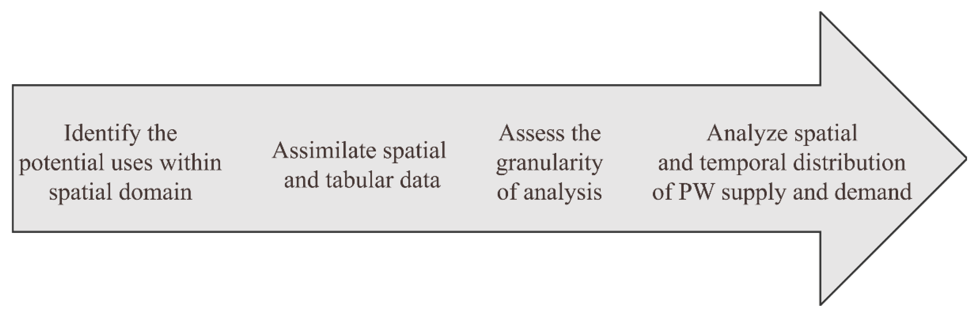
Developing a framework for quantifying the potential demand for reuse of treated PW should include four general steps (Figure 1). First, potential uses for treated PW within the geographic domain should be identified. Spatial and aspatial data on water use from state and federal sources should be assimilated into a geographic information system (GIS). Next, the granularity of analysis should be established at a management decision scale. Lastly, the PW water supply and demand data should be analyzed to illustrate the geographic and temporal distribution for comparison to PW volumes at multiple spatial scales to inform potential locations and management of treated PW.
2.1. Study Location
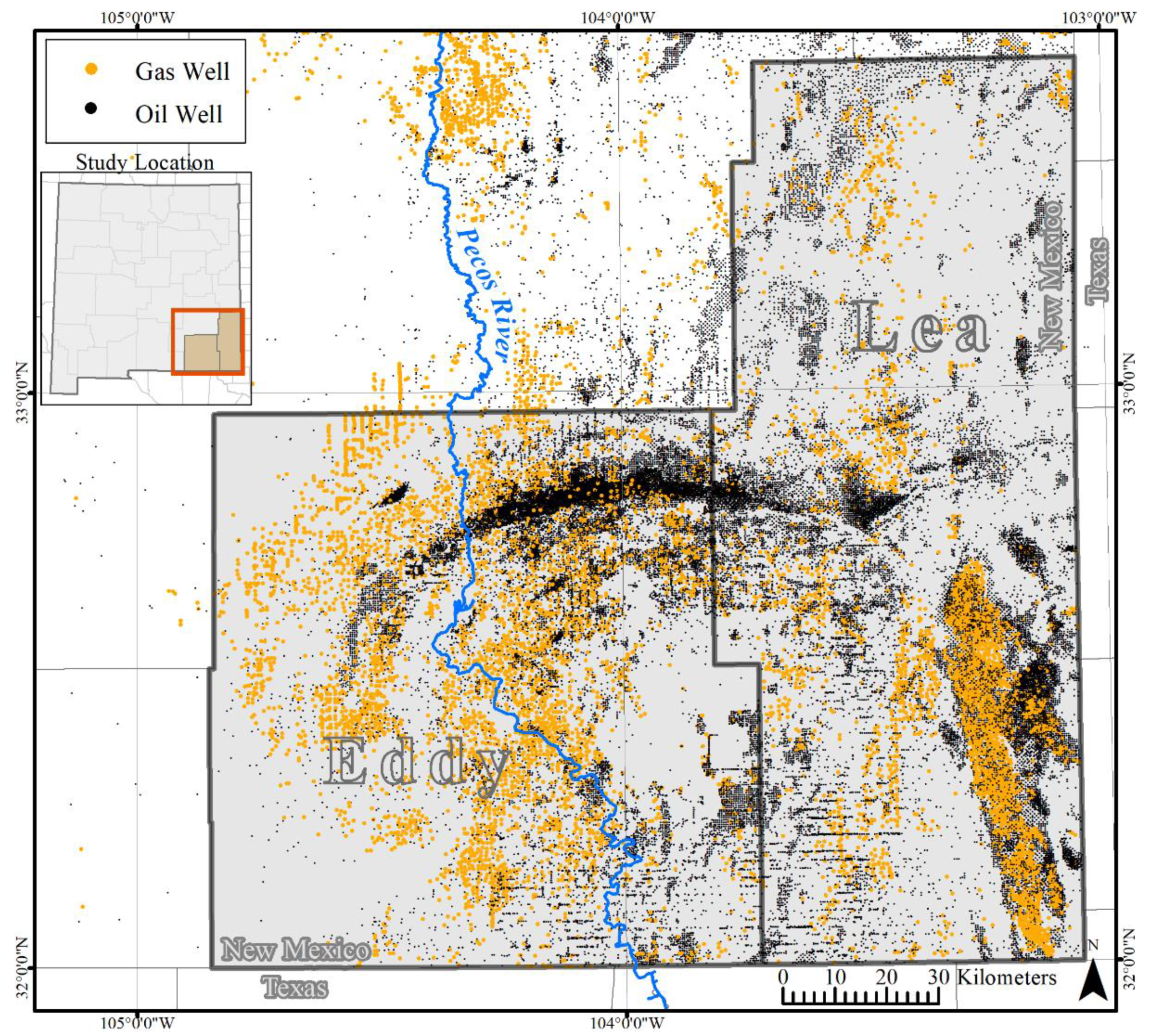
The development of a framework for analyzing PW supply and demand for potential reuse was applied to Eddy and Lea counties in southeastern New Mexico (Figure 2). The counties are representative of regions with decreasing water supply, increasing competition for water uses, and increasing pressure to better manage PW. The two counties are situated on top of the western portion of the Permian Basin and are among the top oil-producing counties in the United States. Eddy County is approximately 4198 square miles and has an estimated population of 58,460. Lea County is approximately 4394 square miles and has an estimated population of 71,070. Both counties share a border with Texas and have common water sources. The Pecos River runs north to south through Eddy County, and is subject to an interstate compact between New Mexico and Texas for surface water deliveries, whereas Lea County does not have a source of surface water. Groundwater comes from the Roswell Basin and the Pecos River alluvial aquifer in Eddy County, and from the Ogallala Aquifer in Lea County. The average annual precipitation is 33.5 cm (13.2 inches) and 37.8 cm (14.9 inches) for Eddy and Lea counties, respectively. The region has seen a shift towards more within-industry reuse of PW [13], where half of the PW generated is recycled for secondary oil recovery. However, the remaining volumes injected into SWD wells and are generating concern over potential of increased seismicity. The major water uses in the two counties are irrigated agriculture, public water supply, power generation, and mining.
2.2. Data Sources
The analysis used data from a variety of sources, including state, federal, and academic research institutes. Water uses by category data were compiled from the New Mexico Office of the State Engineer 5-year water use by category reports from 1990–2015 [14,15,16,17,18,19]. Spatially continuous data illustrating the annual trends in irrigated agriculture for the study site were derived from the United States Department of Agriculture’s Cropland Data Layer dataset for 2008 through 2020 [20]. Using these data allows the estimation of agricultural water demand for different crops.
Historical water demand was examined to illustrate the trends in the major water use categories in Eddy and Lea counties from 1990 through 2015. The data were compiled from New Mexico Office of the State Engineer reports. Time series graphs were produced to show the volumes of combined water withdrawn from surface water and groundwater resources. Similar information can be found for other states through the USGS “Water Use Data for the Nation” website.
Oil, gas, and SWD well data for all of New Mexico were downloaded from the New Mexico Oil Conservation Division FTP website. The data includes geolocation and table attributes describing the unique API identifier, type of well, spud date, drilling direction, pool identification, active status, drilling length, and weblinks to monthly production data. Following a similar preprocessing procedure as Jiang, et al. [21], the initial 127,452 data points were refined by selecting oil and gas wells located in Eddy and Lea counties that had an active or new status and had a measured vertical length greater than zero. The selection reduced the number of data points down to 28,153 wells. Data on the FTP are updated with new wells on a monthly basis.
2.3. Assessment of Granularity
The goal of determining an appropriate spatial scale for information produced through spatial analysis is to provide detail at a level where any increase in granularity provides little additional unique information for the intended purpose. In the case of PW management, the scale of analysis is important because transportation costs and methods play a major role in evaluating the feasibility of reusing treated PW. Analysis should occur at a similar spatial unit where PW management decisions are made to avoid over-aggregation of data, and to minimize the effect of the modifiable areal unit problem [22], where the scale of aggregation and the placement of the polygon zones can dramatically affect the statistics calculated within each polygon.
We derived an appropriate scale through analyzing the descriptive statistics of the average distance from an oil and gas well to the nearest disposal well, the average number of wells within a three-ring radial buffer of each SWD well, and the average distance between disposal wells. First, the descriptive statistics of the distance from active oil and gas wells in relation to active SWD wells in Eddy and Lea counties were calculated using ArcMap 10.8.1, ESRI Redlands, CA, USA [23] to provide a localized characterization of the PW management needs within the study area. The minimum, maximum, and average distance from each oil and gas well to the nearest SWD was measured in Euclidean distance and plotted on a histogram. To understand the concentration of oil and gas wells in relation to the SWD wells, buffers were added around the SWD wells for the three spatial scales and the average number of oil and gas wells within each of these buffers was calculated to consider the number of oil and gas wells that might supply a SWD well. Lastly, we calculated the average distance between active disposal wells. Contiguous polygon grid layers were created at three spatial scales to perform the supply and demand analysis.
2.4. Spatially Distributed PW Supply
Calculating the spatial distribution of PW supply is important for assessing the available volume for meeting beneficial reuse demand. PW supply is affected by numerous variables at the individual well—differences in well type (vertical versus horizontal), the geologic formation, and age of the well. For the current study, we utilize recent PW volume estimates from Jiang, et al. [21] from wells located within the New Mexico portion of the Permian Basin to estimate the spatial distribution of PW supply. Jiang, et al. [21] analyzed 2019 PW volume data from 21,907 oil wells and 2850 gas wells in southeastern New Mexico and found the annual total volume of PW to be 161.6 × 10⁶ m3 and 32.6 × 10⁶ m3 with average annual volumes of 19,500 m3, 3340 m3, 48,330 m3, and 2540 m3 for horizontal and vertical oil wells and horizontal and vertical gas wells, respectively (Table 1).
Potential treated PW supply was estimated for each grid cell at the three spatial scales using a Python script developed during this study. The count of horizontal and vertical oil and gas wells for each grid cell were summed and then multiplied by the average annual volume for each well category as defined in Table 1. The volume of PW in each grid cell was then multiplied by 0.42 to account for the 42% [21] of water that is currently being disposed of in SWD wells and with the assumption that the remainder is being reused within the industry for either enhanced oil recovery or hydraulic fracturing. The product is then multiplied again by 0.5 to assume 50% of the PW can be recovered using thermal desalination processes that are currently being pilot tested at oil and gas facilities in the Permian Basin and from literature [24]. The tabulated volumes of PW supply for each grid cell were joined back to the spatial data to display the spatial distribution on a map.
2.5. Potential Uses of Treated PW
Water demand can be considered in both broad and narrow contexts for potential reuse of treated PW (Table 2). The broad demand in the region, aggregated at the county level, was defined by compiling the water use by category from the New Mexico Office of the State Engineer 5-year water use reports between 1990 and 2015. These reports summarize the groundwater and surface water withdrawals for nine water use categories, and the compilation illustrated the trends in water demand for the two counties.
The narrow categories of demands are more difficult to define because they require local knowledge of specific demands and need to be spatially, and sometimes temporally, disaggregated. For Eddy and Lea counties, several previous publications provide guidance on the potential reuse options already being considered (e.g., [2,12,25]). The list of narrow uses in this study is certainly not exhaustive and conducting a comprehensive analysis of the demand of each use is outside the scope of developing a framework. We provide context for four potential end uses of treated PW in this case study: crop-specific water demand, road dust control, energy production, and streamflow enhancement. The rationality for focusing on these uses is that crop-specific water demand is the largest water use in the region and is exemplary of a spatially distributed demand with a high intra-annual variation. Treated PW for road dust suppression can replace freshwater because there is a low water quality requirement; many of the roads within the oil and gas fields are dirt and potentially have a year-round demand for controlling dust. Power generation has a relatively high water demand and occurs at specific points, which is interesting from a spatial analysis standpoint. Lastly, stream flow enhancement will help meet compact water delivery requirements and augmentation of surface water flow, thus slowing the trend in agricultural land retirement.
2.5.1. Crop Specific Irrigation
Irrigated agriculture represents a large potential demand for treated PW. The trends of irrigated agriculture water demand were estimated using the USDA Cropland Data Layers, the average monthly reference evapotranspiration, and crop coefficients published in the FAO 56 Irrigation and Drainage Paper [26]. Annual USDA Cropland Data Layers from 2008 through 2020 were downloaded, and summary statistics for the total cell count for each crop type and land use/land cover were generated for Eddy and Lea counties to assess the interannual variability of crop types and to determine the most common crops.
Specific crop data from the 2020 USDA Cropland Data Layer were summarized at the three different spatial scales (1.1 miles, 1.5 miles, and 3 miles). Crop raster data were converted to a point file, the points files were appended with a unique grid cell identification, and the associated attribute data were subsequently exported as a .csv file. A Python script was developed to summarize crop and land cover data in the .csv file for each individual grid cell. Crop acreage was calculated by first by multiplying the cell count by 900 m2 (30 m by 30 m cells) for each crop and then multiplying the product by 0.000247105 to convert square meters to acres.
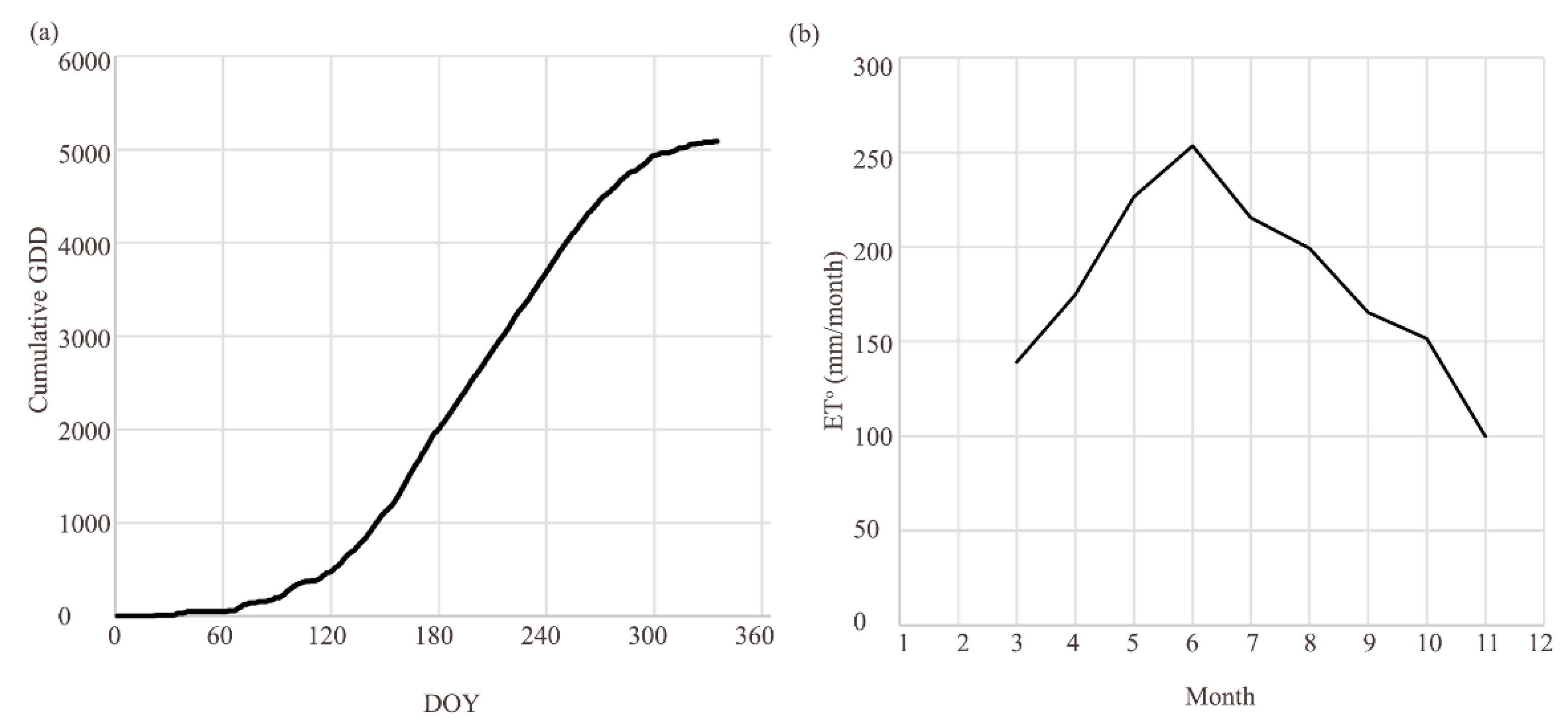
Using cumulative growing degree days (GDD), at base 50 as an indicator of the active growing season (Figure 3a), agricultural water demand in Eddy and Lea counties occurs primarily during the 8-month growing season from March through November, with most of the water demand occurring between May and September when atmospheric water demand is greatest. The monthly volume of water for each crop type for each cell was calculated by multiplying published crop coefficients by the average monthly reference evapotranspiration from the New Mexico State University Artesia Science Center weather station from 2021 (Figure 3b). The individual crop water demand was then summarized for each grid cell for the three spatial units.
2.5.2. Road Dust Suppression
Demand for water use as a dust suppressant on unpaved roads in Lea and Eddy counties was estimated using road centerline data from the New Mexico 911 Program and the 2010 U.S. Census Bureau. The New Mexico 911 Program dataset includes road centerlines of primarily paved roads for emergency response, and they are frequently updated as new developments are built. The U.S. Census data contain several categories of roads, including both paved and unpaved roads, and is updated every ten years. A visual inspection of both datasets revealed a general misclassification of the U.S. Census roads in the “Local Neighborhood Road, Rural Road, City Streets” (S1400) class, which is generally paved roads. The Census data misclassified most unpaved roads in Eddy and Lea counties as members within the “Local Neighborhood Road, Rural Road, City Streets” class.
We applied a spatial filter to determine the unpaved roads in both counties by assuming roads in the NM 911 dataset were paved, subtracting those roads from the Census roads dataset, and assuming the remaining roads as being unpaved. Census road data represents road paths, with lines representing both sides of divided highways and on ramps, where the New Mexico 911 layer only included one centerline for divided highways. As such, an additional filter was necessary to exclude the divided highway and on-ramp road segments not captured by the co-location filter. A limitation to this analysis is that the Census data were prepared for the 2010 Census, prior to the surge in oil and gas production in the region; thus, it is likely more unpaved roads were established since the dataset was released.
Following road segment selection, the total length of unpaved roads was calculated in GIS within each of the three spatial units. Although the frequency of a dust suppression treatment for a road segment varies for many reasons (e.g., increased construction, funding, proximity to densely populated areas, etc.), we assume each segment can be treated one time per year to estimate the volume of treated PW demand for dust suppression. Assuming a 15-foot-wide (4.57 m) road and a conservative dust suppression application rate for water of 2 mm per unit area from Yonkofski, et al. [27], we estimated 3388 gallons/mile (7.969 m3/km) for treated PW demand for dust suppression. While these assumptions may not be precise in terms of estimating actual volumes of water demand for dust suppression, management decisions could be informed by displaying the results on a map, illustrating the relative spatial distribution of demand, and they can be easily adjusted by multiplying the miles by a different application rate.
2.5.3. Power Generation
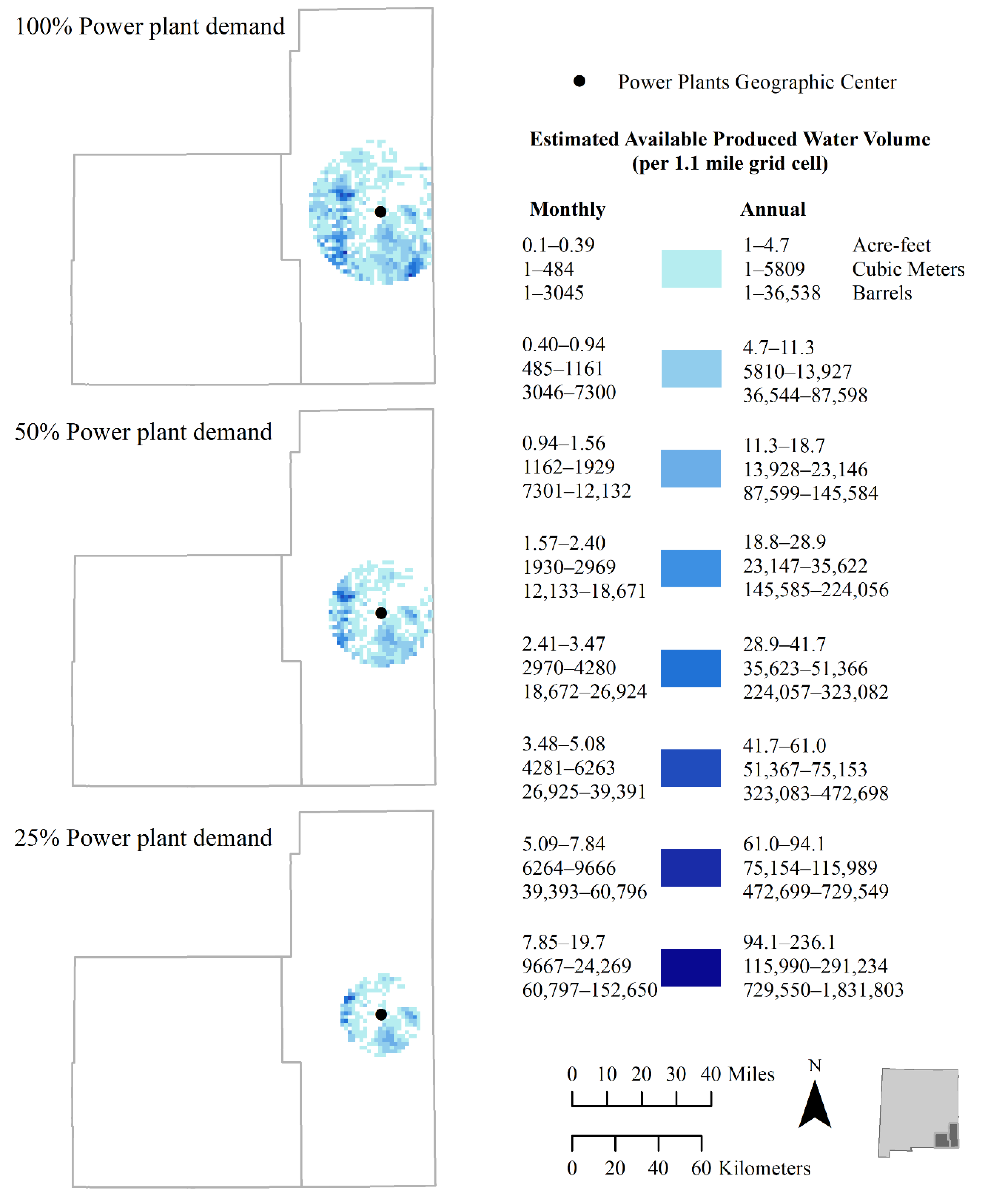
Three thermal-electric power plants with a power generating capacity of 1414 MWe currently operate in Lea County and are located within 5 km (3.1 miles) of each other. The Hobbs Generating Station has a capacity of 682 Megawatt electric (MWe), the Cunningham Steam Turbine Power Plant has a capacity of 519 Megawatt electric Mwe, and the Maddox Gas Plant has a capacity of 213 MWe. We could not locate any water use reporting by individual plants; therefore, we assume these three power plants account for the 5,516,122 m3 (4472 acre-feet) of total water withdrawals reported in the 2015 New Mexico Office of the State Engineer Water Use by Category report [19]. Since the power plants are in relatively close proximity to each other, we calculated a geographic center of the three plants and based demand off that one point. There are no thermal-electric power plants with cooling towers in Eddy County.
Using the results of the estimated supply analysis, a Python script was developed to assess a collection area required to meet different levels of demand. The script requires two point files: one with the location of intended use, i.e., the geographic center of the three power plants, and a point file that includes the location of supplies and associated volumes of treated PW supply. The center point of each 1.1-mile grid cell was used in the analysis. The Euclidean distance from each supply point to the demand point was calculated and sorted in order of the least distance to the greatest distance. The script is iterated ordinally through each supply point until the sum meets the desired demand. The selected points were output as a .csv file and joined back to the supply grid in ArcMap using a unique grid ID. The supply area was calculated and mapped for meeting 25, 50, and 100% of the power plants demand.
2.5.4. Streamflow Enhancement
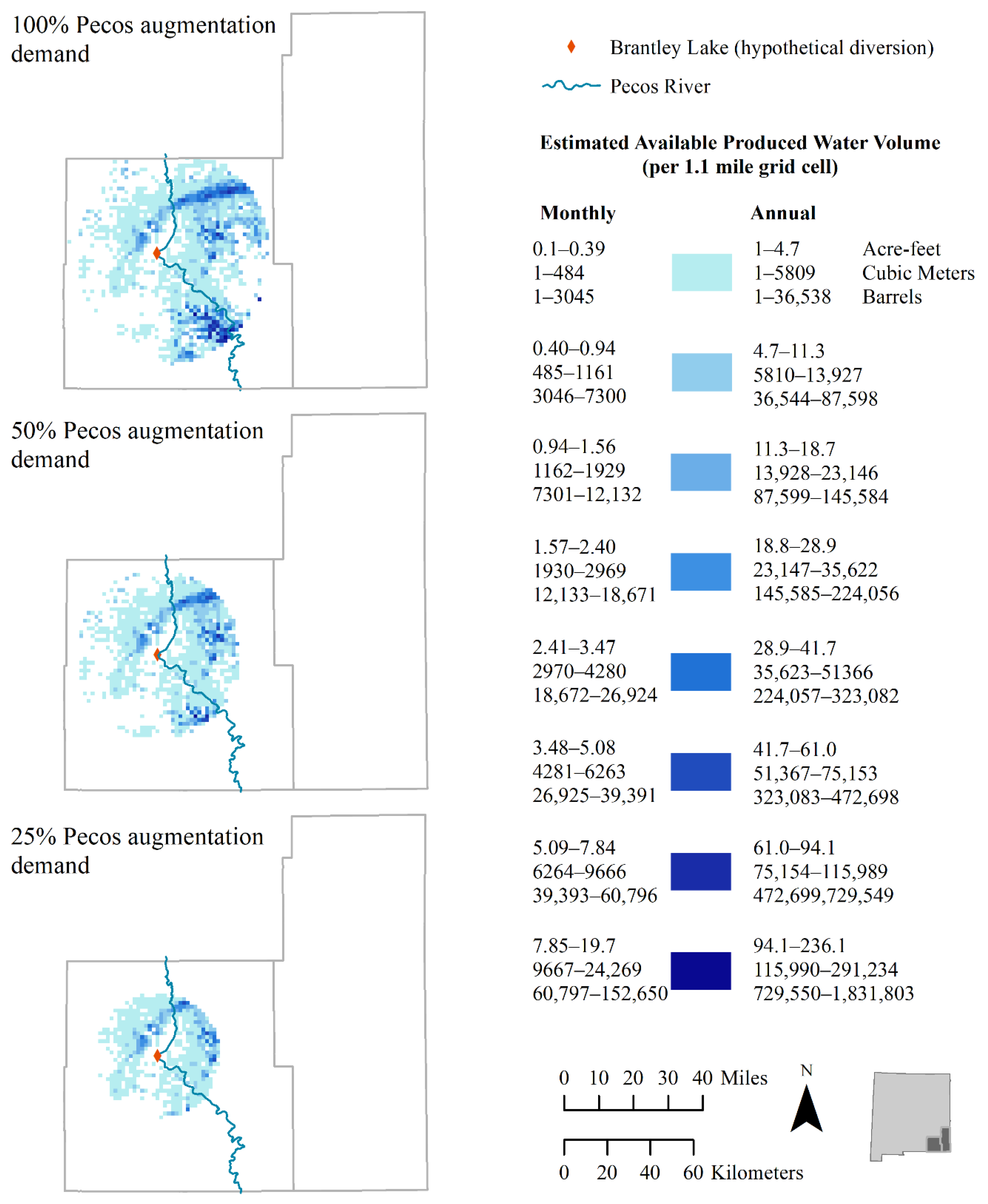
Another potential use of treated PW is to augment the Brantley Reservoir in Eddy County, thus providing additional water for meeting Pecos River Compact deliveries to Texas, increasing environmental flows, and providing additional irrigation water. In many years, the shortfall to meeting this water requirement is 10,000 to 50,000 acre-feet/year (AFY) [28], although New Mexico has a 161,000 acre-foot credit as of 2022 [29].
The collection area needed to meet demands for streamflow augmentation was calculated using the same process and Python script described in the ‘Power water demand’ section. Based on the Supreme Court order, the assumption of a demand of 12,334,800 m3 (10,000 acre-feet) per year for augmenting the flow of the Pecos River was used for assessing the collection area for the supply. The most beneficial point of discharge may be before the Brantley Reservoir, where augmentation could be accepted year-round with acceptable dilution factors, and thus was used as the point of demand. The analysis was run to identify the collection area for meeting 25%, 50%, and 100% of the river augmentation demand requirement.
2.5.5. Other Potential Uses
In semiarid lands, the need for water presents many other opportunities for potential reuse of treated PW not analyzed in this study. Hydrogen production in New Mexico is gaining attention after the Hydrogen Hub Development Act was introduced in early 2022. Carbon sequestration is another emerging interest in New Mexico which has a high variability in water volume requirements depending on the technology being utilized. Mining activities could utilize treated PW to reestablish a defined vegetative cover to meet requirements for mining bond releases. Municipal water is one of the largest water uses in both Eddy and Lea counties; however, it would likely be one of the least likely uses for treated PW because of the concern of public perception and regulatory requirements. Another option would be to indirectly use treated PW for municipal water demand by injecting it into local groundwater aquifers to offset their withdrawal for use at the treatment facility.
3. Results and Discussion
The volume results from this analysis are presented in different units relevant to the various audiences and to facilitate a better cross-discipline understanding (Table 3). Agriculture in New Mexico typically measures water volume in terms of acre-feet, the oil and gas industry typically measures volume in barrels, and cubic meters is common for the scientific community.
The spatial and temporal differences between irrigated agriculture, dust suppression, power generation, and river augmentation—spatially distributed demand versus point demand—made it difficult to produce a map summarizing the total potential demand per grid cell. Therefore, two different approaches were used for estimating the potential demand. The first approach used spatially disaggregated data to estimate the potential demand for agriculture and dust suppression per grid cell. The second approach used a single point of demand for either power plant or river augmentation demand to calculate the collection area needed to meet different percentages of the total demand based on the minimum distance to the sources of PW. Agriculture had the largest demand of all the potential uses of treated PW; however, the demand varied in time and location. A limitation is that neither of these two analyses included a treatment facility or transportation infrastructure location.
Two pieces of critical information are still needed to improve the usefulness of the methods and information presented in this study. The location of a PW treatment facility is a critical need for improving the usefulness of the information presented in this study because it would serve as both a collection and distribution point. Once a treatment facility is located, the methodology presented could be improved and optimized for flows into, and out of, the treatment facility with the associated costs. The location of pipeline infrastructure used for transporting raw PW and treated PW would be a dramatic improvement for modeling the PW management, as it could effectively reduce the relative distance to the point of supply to the point of demand.
3.1. Broad Historical Water Demand
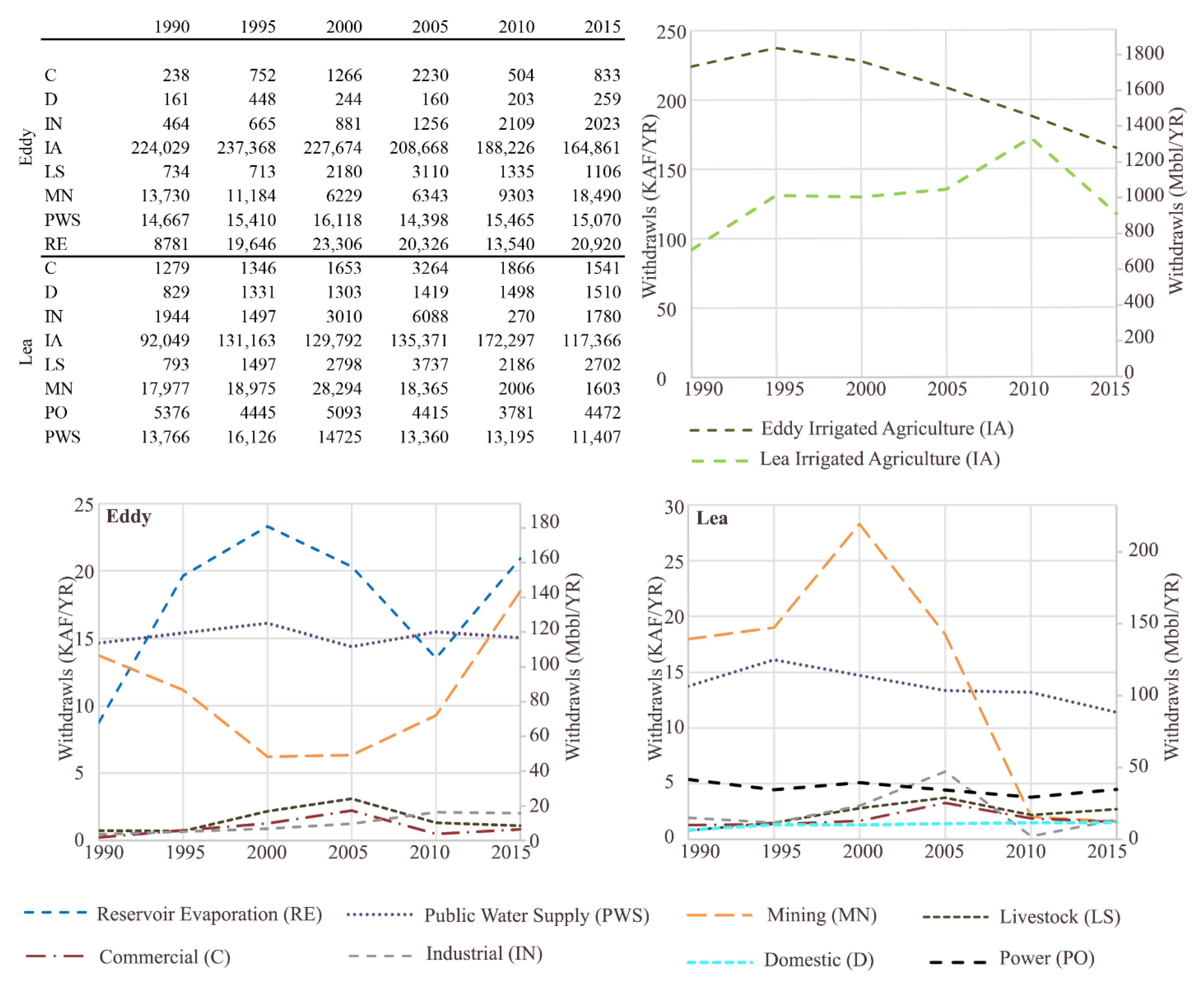
The broad historical demand provided a reference point for developing the framework. The trends of broad water use demand for Eddy and Lea counties show that the largest water use by category is irrigated agriculture (Figure 4), which is an order of magnitude larger than the second largest water use category and more than two orders of magnitude larger than the smallest categories. Reservoir evaporation accounts for a substantial portion of the water use in Eddy County but is zero in Lea County. Public water supply and mining are the next two largest water use categories in both counties. Agricultural water demand is decreasing in both counties, a reflection of the retirement of agricultural land in Eddy County to meet the Pecos River Compact deliveries and a rapidly decreasing groundwater supply in Lea County [30]. The mining category includes water used in potash, coal, metals, and oil and gas, as well as water used for watering vegetation during mine reclamation. There is a 179% decline in the mining water use category in Lea County from 2000 until the present, despite the increase in oil and gas activity during the same period. Some possible causes for this decline include errors in data reporting, mining water being imported from Texas, water reuse and recycling, and/or a reduction of potash mining activity. Tracking the water used within the oil and gas industry remains a challenge in New Mexico even as new regulations require the type of source water used in drilling.
3.2. Granularity
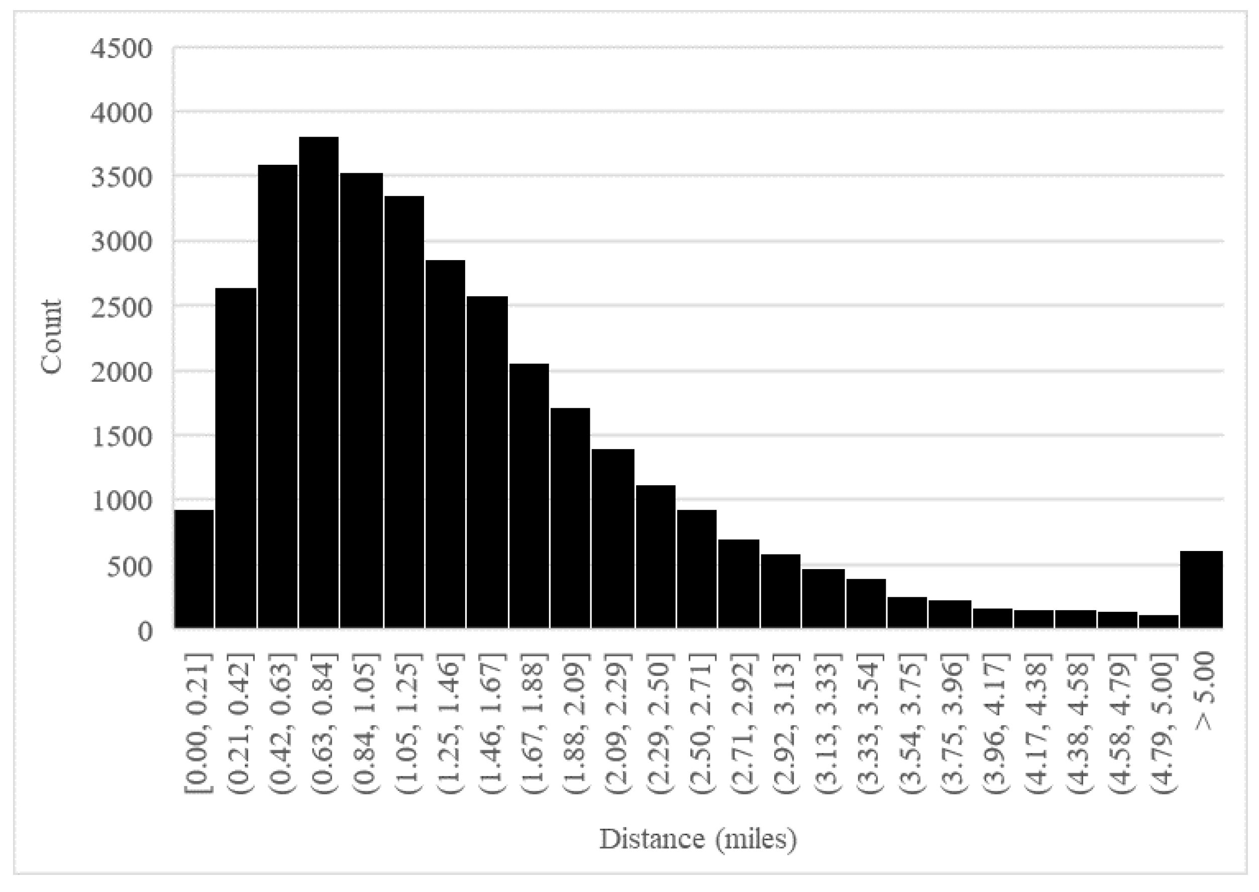
An assessment of the granularity was used to determine three spatial scales of analysis to be used within the framework for analyzing the spatial distribution of PW supply and demand. Descriptive statistics were calculated for the minimum distance from each oil or gas well to the nearest SWD well for each county, and they also considered all the wells in both counties because some wells may be in one county, while the nearest SWD well could be in the other county. The results suggest a majority of oil and gas wells have a SWD well within two miles. The mean distance between oil and gas production wells and the nearest SWD well was 1.51 miles and 1.53 miles for Eddy and Lea counties, respectively. The data do not follow a normal distribution and are skewed to the right of the histogram, suggesting the use of the median distance as a better representation of the central tendency (Figure 5). The median distances were 1.1 miles for Eddy County, 1.34 miles for Lea County, and 1.21 miles combined (Table 4). The minimum distance was less than 0.01 miles, likely because some production wells have an onsite SDW. The maximum distance was 16.06 miles in Eddy County and 8.02 miles in Lea. One shortcoming of this analysis is that it does not consider production wells or SWD wells on the other side of the Texas border, which could potentially shift the statistics. However, even if those wells were included, there are few data readily available describing how much PW is moved across the state borders. Based on the results of the descriptive statistics, we produced three grid scales (1.1, 1.5, and 3.0 miles) which capture the distance between oil and gas wells to SWD wells for approximately 45%, 62%, and 91% of the wells in Eddy and Lea counties, respectively.
The average number of oil and gas wells in proximity to a SWD is also important to consider because SWD wells could be considered good collection points since they already have pipeline and/or road infrastructure networks built to receive PW. The average number of oil and gas wells within three radial buffers of SWD wells was calculated (Table 5). The average number of wells within 1.1 miles of SWDs was approximately 2, with a maximum of 8. There was an average of approximately 2.7 wells within 1.5 miles with a maximum of 9. At 3 miles, the average is approximately 6.7 wells within the buffer and a maximum of 21. The 3-mile buffer captures 91% of the oil and gas wells in Eddy and Lea counties. The average distance between SWD wells was 1.35 miles with a maximum distance of 8.7 miles.
In the context of PW management, assessing the granularity provides a systematic method for determining a scale useful for data aggregation to address challenges in transportation needs. Transportation of PW through trucking and/or pipelines is often discussed in scientific literature and at industry meetings as one of the main costs of PW management. A 2019 report by the Ground Water Protection Council provides some insight, where an estimated 20-mile roundtrip was used as an example for trucking distance from source water to the well location [31]. Our analysis improves on previous analyses that aggregated PW volumes at the township scale of 6-mile grid [6,32], which is insufficient for making management decisions.
3.3. Produced Water Supply
The estimated annual supply of treated PW was 22,855,016 m3 (18,536 acre-feet) in Eddy County and 22,605,859 m3 (18,334 acre-feet) in Lea County. The estimated annual total available volume of treated PW in the two counties was 45,460,875 m3 (36,870 acre-feet) which is much lower than the total reported volumes because of the assumptions of 58% reused within the oil and gas industry and a 50% water recovery through thermal desalination processes. These volumes could increase or decrease depending on the water quality, treatment recovery, and the volume of water reused within the oil and gas industry for hydraulic fracturing and enhanced oil recovery.
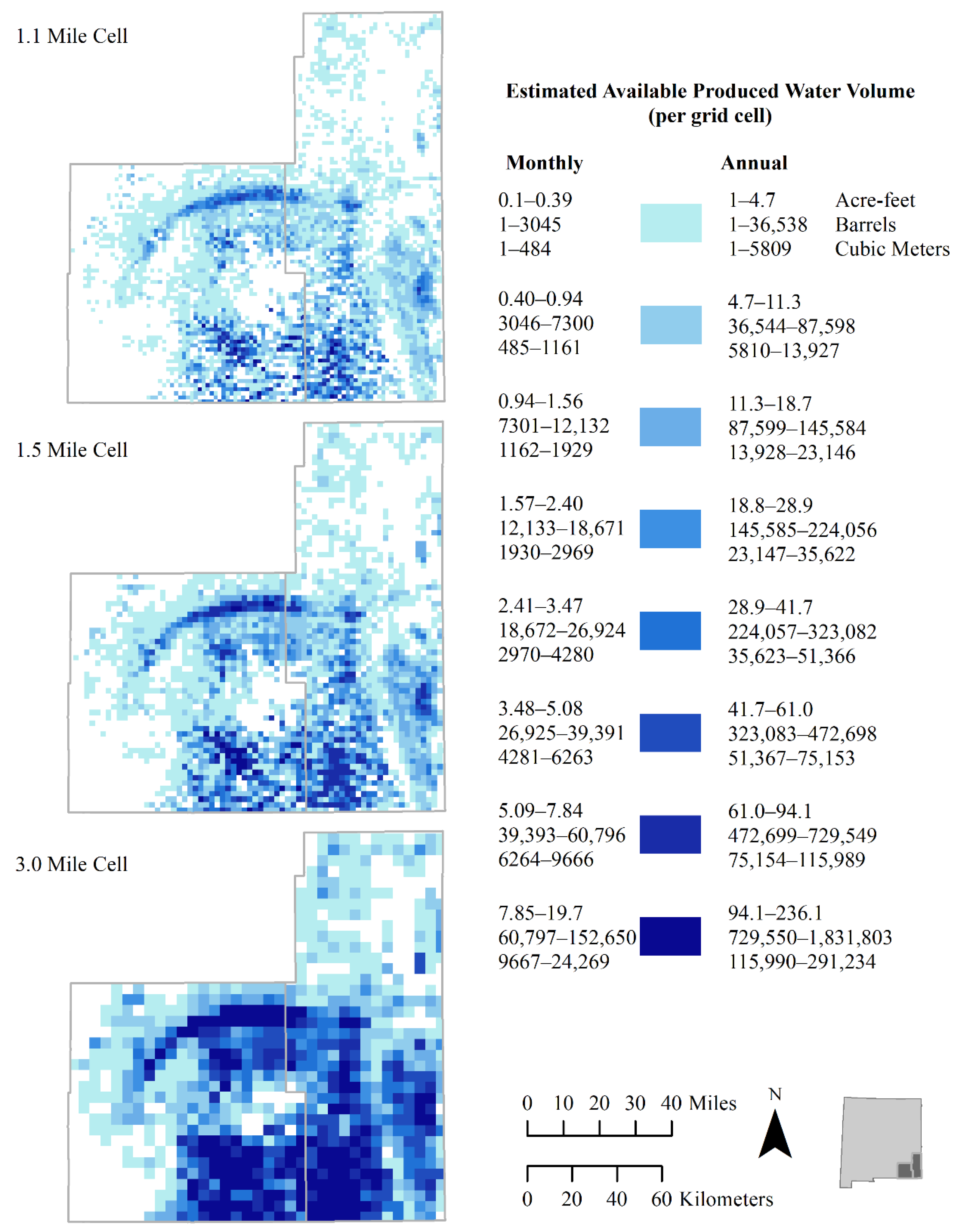
The estimated supply of available PW is variable throughout the study region. Maps were produced to illustrate the spatial variability of supply in Eddy and Lea counties at three grid scales (Figure 6). The symbology was first classified using the Jenks natural breaks method on the 1.1-mile grid data in order to equally distribute map errors, and then the largest class was increased to capture the effect of increased volumes at the 3-mile grid resolution. The maps illustrate the effect of aggregation on resolving the granular data—as the grid cell size increases, the ability to resolve the location of supply decreases. The higher spatial resolution shows more of the checkerboard pattern from created by the differences in land ownership and management status. The symbology was deliberately held constant for the different grid cell sizes to further illustrate this point. The largest volume class in the symbology has a range larger than the other seven classes combined to capture the increased aggregated volume at the 3-mile grid resolution creating map errors in the 1.1-mile grid map for the largest volume class. There are grid cells in the 3-mile where the lower classes are still represented, and reclassifying the symbology would increase the error in the lower volume classes. The result of the different levels in aggregation provides evidence that assessing the granularity is important for producing information at an appropriate scale for PW management decisions; thus, the remaining analyses are presented at the 1.1-mile grid cell.
An important point that should not be understated is the cost of treating the estimated volume of water. The PW treatment costs depend on the PW quality and water quality requirements of end users. PW in the Permian Basin can contain approximately 1400 compounds, including BTEX (benzene, toluene, ethylbenzene, and xylene), various suspended particles, dissolved solids, soluble and insoluble organic compounds, naturally occurring radionuclides, and production chemicals (e.g., acids, corrosion inhibitors, surfactants) [33]. The average total dissolved solids (TDS) concentration of PW in the Permian Basin is approximately 90–100 g/L [34], which requires thermal distillation treatment. It is estimated that the costs to recover a net 45,460,875 m3 treated PW could be between USD 266 and USD 496 million, with unit treatment costs ranging between USD 2.92/m3 and USD 5.45/m3 for PW with a salt level of 90 g/L from Osipi et al. [35] and Xu et al. [36]. Additional information on the costs and removal efficiencies of technologies for treating various qualities of PW can be found in Ma et al. [37] and Geza et al. [38]. Although providing a complete cost analysis is outside the scope of this study, some additional context can be provided by highlighting the SWD well disposal costs for the same volume of PW would likely be between USD 71 million and USD 715 million using the disposal cost for SWD wells ranging from USD 0.25/barrel ($1.57/m3) and USD 2.50/barrel ($15.72/m3) published in an industry magazine [39].
The annual total PW volumes in this study are underestimated by approximately 9.8% compared to data reported by the New Mexico Oil Conservation Division (NMOCD) for the similar time period. NMOCD reported 238,853,304 m3 (193,638 acre-feet) in Eddy and Lea counties in 2021 compared to the 216,563,845 m3 (175,571 acre-feet) estimated in this study. PW volume is constantly changing throughout the production cycle and a more elegant process such as a dynamic hybrid agent-based and system dynamics model as discussed in Langarudi et al. [40] could increase the accuracy of the estimates for improving management decisions. Another improvement to this analysis would be the inclusion of decline curves for each well based on the geologic formation the well is producing from.
3.4. Irrigation Water Demand
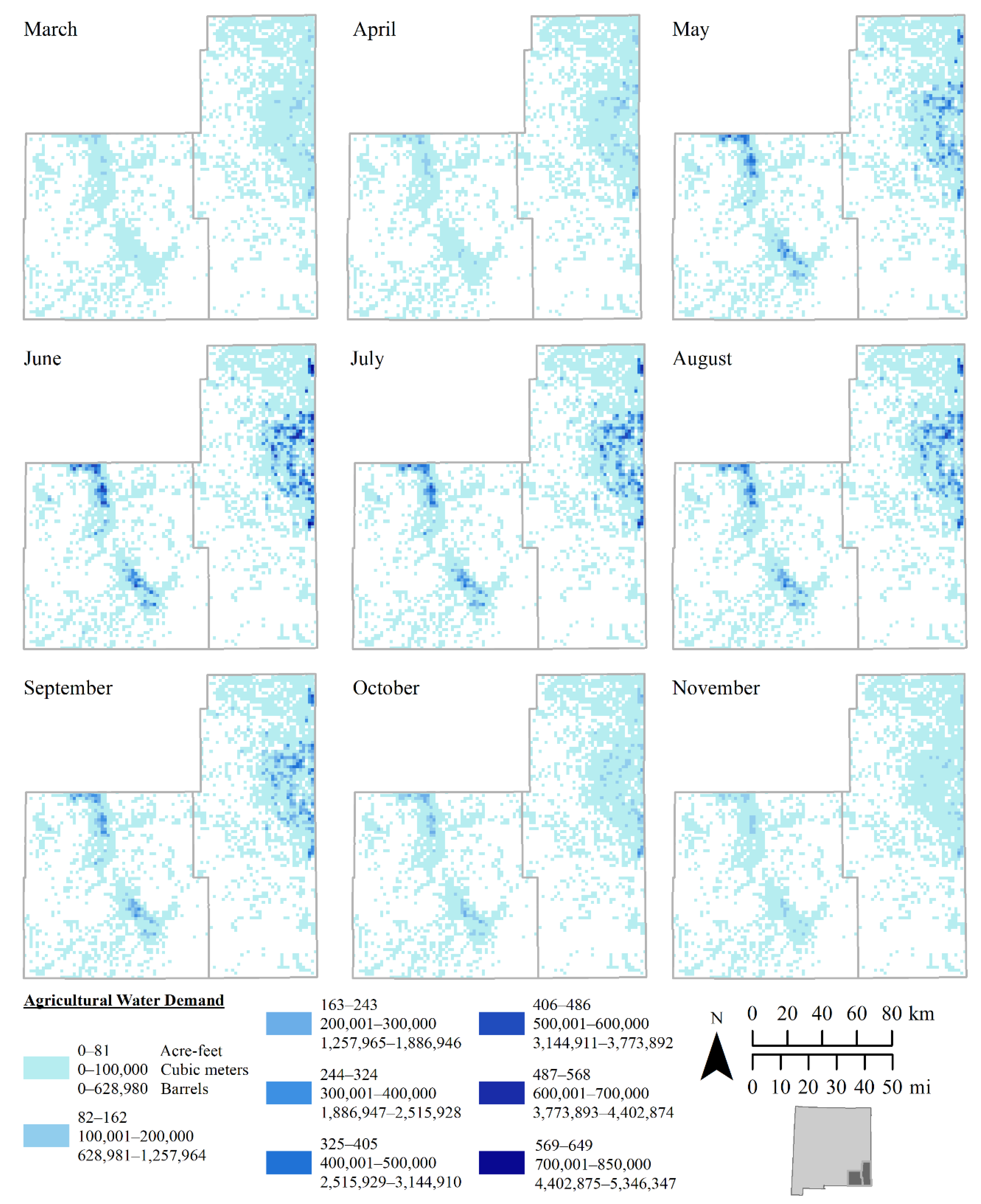
The irrigated agricultural water demand for Eddy and Lea counties was estimated using growing degree days, crop coefficients, and local reference evapotranspiration values. The growing season primarily occurs between March and November—the highest intensity of irrigation water demand occurring between June and August (Figure 7). The highest demand for a grid cell was 649 acre-feet in June and the mean demand per grid cell was 40.2 acre-feet. Approximately 23% of the grid cells had <1 acre-feet of demand, suggesting misclassification in the USDA imagery. Alfalfa was the dominant crop for Eddy County and cotton was the dominant crop in Lea County; alfalfa is showing a declining trend. The spatial distribution of the irrigation demand is focused along the Pecos River in Eddy County and where numerous center pivots pump groundwater from the Ogallala aquifer in eastern Lea County. The highest demand occurs in June through August at the peak of the growing season.
The estimated total annual irrigated agriculture water demand is 170,944 acre-feet and 343,915 acre-feet for Eddy and Lea counties. The estimate for Eddy County is similar to the annual estimates of 164,861 acre-feet of consumptive use provided in Magnuson et al. [19]; however, the estimate for Lea County is more than double the 117,366 acre-feet provided in Magnuson et al. [19]. It is unclear as to why the Lea County estimate diverges so much from the official State report since the estimates are both made using the USDA Crop Data Layer as a basis. Two main differences are the purpose of the reports and the year of data used. Magnuson et al. [19] reported water use only in terms of withdrawals from surface and groundwater, whereas the current study is looking at total crop water demand. Another difference could be the current study was run for 2021, whereas Magnuson et al. [19] based their report on 2015 data and note that the eastern part of New Mexico received precipitation that was significantly higher than average, which would cause the withdrawal values to be lower.
Nonetheless, the trends in agriculture production suggest that Lea County would have a much larger irrigation water demand. In 2018, the acres of land in farms in Eddy County (1,087,902 acres) were 78% less than the land in farms in Lea County (1,938,321 acres), and the total agriculture income was USD 109 million for Eddy and USD 226 million for Lea [41]. Although the larger livestock population in Lea accounts for some of the differences in agricultural income, the larger agriculture acreage reported by NMDA suggests Magnuson et al. [19] could be underestimating the consumptive use in Lea County. In our analysis of irrigated acreage based on the 2020 Cropland Data Layer, we estimate that Eddy County had 37,538 acres and Lea County 73,991 acres. The relative intensity of demand presented in this study is a useful starting point for informing PW management decisions, and the future goal should be working towards better quantifying absolute volumes of irrigation water demand. Additionally, future efforts in quantifying irrigation water demand should include spatiotemporal precipitation data such as the gridded PRISM climate data.
3.5. Dust Suppression
The purpose of using water for dust suppression is to meet an optimum moisture and compaction goal [42]; however, dust suppression on rural roads is a challenge in arid environments because unpaved roads produce dust given the persistent dry conditions. Treated PW could provide a viable alternative for dust suppression because the sources, assuming PW treatment facilities would be located within the oil and gas fields, would be closer to the haul roads, the salt in brackish water helps bind the clay to roadbeds—improving the longevity of the treatment—and the demand for dust control is year-round.
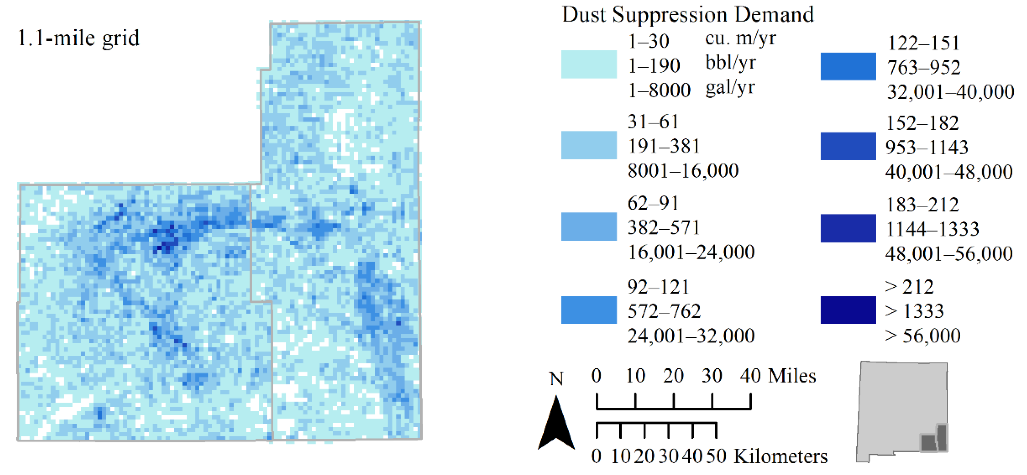
An estimate of 9884 miles in Eddy and 8776 miles in Lea County have a potential treated PW demand for dust suppression. Using the assumptions of treating every mile at least once annually and at a rate of 3388 gallons/mile (7.969 m3/km), the total dust suppression demand was estimated to be 33,488,465 gallons/year (126,768 m3/year) for Eddy County and 29,444,153 gallons/year (111,458 m3/year). The dust suppression frequency is difficult to predict and the assumption of one treatment per year for every mile is likely conservative for some locations while likely overestimated for grid cells with a lower concentration of road segments. The demand is spatially distributed throughout both counties and the mean demand is approximately 10,072 gallons/year for Eddy and 8405 gallons/year for Lea County per 1.1-mile grid cell (Figure 8). The map legend breaks are at 8000-gallon equal intervals, representing an approximate two fully loaded 4000-gallon tanker trucks. The grid cells with the highest demand occur along the edge of the Delaware Basin where there is also a high concentration of oil and gas wells, and therefore more roads. The estimated dust suppression water demand could be improved with more specific information on the width of the roads, the average daily traffic, and road quality.
3.6. Power Plant Demand
Energy and water are closely linked through the concept of energy–water nexus, which includes oil and gas production as well as electricity generation. Thermoelectric power generation requires large volumes of water for steam generation and cooling. The total volume of power plant water demand was assumed to be 5,516,122 m3 (4472 acre-feet), and the minimum distance to a grid cell centroid was used to cumulatively calculate the area required to meet 100, 50, and 25% of the demand based on the supply estimates (Figure 9).
The collection area was 821 mi2, 455 mi2, and 252 mi2 for meeting 100, 50, and 25% of the demand. The mean annual supply per grid cell within the calculated collection area was 8113.5 m3 (2,143,360 gallons), 7304.8 m3 (1,929,724 gallons), and 6642.7 m3 (1,754,816 gallons) for meeting 100, 50, and 25% of the demand. A limitation to the method used for determining the collection area for meeting the demand for the power plant water or the Pecos River augmentation demand is that it is not optimized for clustering of PW sources, potential anisotropy in the data, the quality of the PW, or pipeline delivery networks that could change where the water would be sourced from and the total collection area.
3.7. Pecos River Augmentation
The Brantley Reservoir was used as the hypothetical point of delivery for treated PW into the Pecos River. The collection area to meet 100, 50, and 25% of the demand is 1488 mi2, 1048 mi2, and 667 mi2, respectively (Figure 10).
The mean annual volume for the 100, 50, and 25% collection area is 8.1, 5.8, and 4.5 acre-feet/1.1-mile grid cell. Many of the grid cells have less than 2 acre-feet of PW annually, which alludes to the difficulty in establishing a collection area while balancing the logistical challenges of transporting water from the oil and gas wells to a PW treatment plant and then to a delivery point on the Pecos.
Similar to the power plant demand analysis, this analysis was not optimized for clusters of supply, nor did it include a pipeline network. Any planning for a system to meet these demands should explore these considerations. Another consideration for the Pecos River augmentation would be setting multiple points of delivery to meet the demand.
Any release to the Pecos River would need to be in coordination with the Interstate Stream Commission (ISC), Carlsbad Irrigation District (CID), the Pecos Valley Artesian Conservancy District (PVACD), and the Fort Sumner Irrigation District (FSID). Supplementation of the Pecos River Basin could benefit the National Environmental Policy Act (NEPA) and the Endangered Species Act (ESA). In years where there is an abundant supply in the reservoirs, treating PW for river augmentation would not be an optimal beneficial use.
The potential use of treated PW for augmenting stream flows in New Mexico might become economically feasible as treatment and transportation costs approach the current costs associated with meeting compact requirements. In 2003, New Mexico implemented an agricultural land retirement program that cost the state more than $100 million to purchase water rights in order to increase the deliveries by an average of 10,000 acre-feet per year. Another costly practice currently employed is to pump groundwater in order to meet Pecos River Compact deliveries in years of delivery shortages, which has the negative impact of lowering the water table and affecting the freshwater supply for agriculture. Thus, using treated PW to help meet the Pecos River Compact requirements could relieve some of the pressure on the state and irrigation districts that are responsible for ensuring the deliveries to Texas.
4. Conclusions
A generalized framework was developed for estimating PW supply and potential demand for treated PW reuse using Eddy and Lea counties, New Mexico as a case study. The framework is transferable and can be adjusted to assess the demands of other potential uses of treated PW not included in this study. The granularity of analysis for the study area was determined to be a 1.1-mile grid using median distances between oil and gas wells and the nearest SWD well. Comparing the results of treated PW supply data aggregated at three different spatial scales illustrated the importance of running an analysis at a scale useful for capturing information at the PW management scale as aggregation can hide information that is useful for making decisions. We estimated the total available supply of treated PW to be 45,460,875 m3 (36,870 acre-feet) for the two counties. Demand was estimated and spatially aggregated to a 1.1-mile grid for four potential options for treated PW reuse. In our analysis, irrigated agriculture was the only potential use that required a temporal element. Future work should integrate the location of a PW treatment plant and pipeline infrastructure to the framework for optimizing the supply and demand relationship leading to improved PW management. The oil and gas industry is dynamic;, therefore it is recommended to use the methodology presented in this study as part of an iterative workflow for PW management.
Author Contributions
Conceptualization, R.P.S., L.P. and P.X.; investigation, R.P.S. and L.P.; data curation, R.P.S. and L.P.; writing—original draft preparation, R.P.S.; writing—review and editing R.P.S., L.P. and P.X.; visualization, R.P.S. and L.P.; supervision, P.X. All authors have read and agreed to the published version of the manuscript.
Funding
This research was funded in part by the New Mexico Universities Produced Water Synthesis Project through the New Mexico Water Resources Research Institute and by the New Mexico Produced Water Research Consortium.
Data Availability Statement
All processed data used in the study have been shown in the article. Raw data may be available on request from the corresponding author.
Acknowledgments
We would like to thank the New Mexico Water Resources Research Institute and the members New Mexico Produced Water Research Consortium for supporting this research.
Conflicts of Interest
The authors declare no conflict of interest.
References
- Scanlon, B.R.; Reedy, R.C.; Male, F.; Walsh, M. Water Issues Related to Transitioning from Conventional to Unconventional Oil Production in the Permian Basin. Environ. Sci. Technol. 2017, 51, 10903–10912. [Google Scholar] [CrossRef] [PubMed]
- Scanlon, B.R.; Reedy, R.C.; Xu, P.; Engle, M.; Nicot, J.P.; Yoxtheimer, D.; Yang, Q.; Ikonnikova, S. Can We Beneficially Reuse Produced Water from Oil and Gas Extraction in the Us? Sci. Total Environ. 2020, 717, 137085. [Google Scholar] [CrossRef] [PubMed]
- Roose, R. New Mexico Environment Department Produced Water Act Implementation Update; Water and Natural Resources Interim Committee: Santa Fe, NM, USA, 2020. [Google Scholar]
- Khatib, Z.; Verbeek, P. Water to value-produced water management for sustainable field development of mature and green fields. In Proceedings of the SPE International Conference on Health, Safety and Environment in Oil and Gas Exploration and Production, Kuala Lumpur, Malaysia, 20–22 March 2002. [Google Scholar]
- Veil, J. Produced water volumes and management practices for 2017. In Proceedings of the GWPC UIC Conference, San Antonio, TX, USA, 16–18 February 2020. [Google Scholar]
- Cather, M.; Chen, D. Improving and Updating of the Nm Produced Water Quality Database: Summary of New Mexico Produced Water Database and Analysis of Data Gaps; New Mexico Water Resources Research Institute: Las Cruces, NM, USA, 2016. [Google Scholar]
- New Mexico Produced Water Research Consortium. New Mexico Produced Water Data Portal. Available online: https://nm.waterstar.org/ (accessed on 12 January 2022).
- Scanlon, B.R.; Ikonnikova, S.; Yang, Q.; Reedy, R.C. Will Water Issues Constrain Oil and Gas Production in the United States? Environ. Sci. Technol. 2020, 54, 3510–3519. [Google Scholar] [CrossRef] [PubMed]
- Arbués, F.; Garcıa-Valiñas, M.Á.; Martínez-Espiñeira, R. Estimation of Residential Water Demand: A State-of-the-Art Review. J. Socio-Econ. 2003, 32, 81–102. [Google Scholar] [CrossRef]
- Yang, B.; Zheng, W.; Ke, X. Forecasting of Industrial Water Demand Using Case-Based Reasoning—A Case Study in Zhangye City, China. Water 2017, 9, 626. [Google Scholar] [CrossRef] [Green Version]
- Ye, Z.; Chen, Y.; Li, W. Ecological Water Demand of Natural Vegetation in the Lower Tarim River. J. Geogr. Sci. 2010, 20, 261–272. [Google Scholar] [CrossRef]
- Sabie, R.; Fernanld, A. The Feasibility of Utilizing Produced Water to Improve Drinking Water Supply in Southeastern New Mexico; New Mexico Water Resources Research Institute: Las Cruces, NM, USA, 2016. [Google Scholar]
- Thomson, B.M.; Chermak, J.M. Analysis of the Relationship between Water, Oil & Gas in New Mexico: Investigation of Past and Future Trends; New Mexico Water Resources Research Institute: Las Cruces, NM, USA, 2021. [Google Scholar]
- Wilson, B.C.; Lucero, A.A. Water Use by Categories in New Mexico Counties and River Basins, and Irrigated Acreage in 1990; New Mexico Office of the State Engineer Technical Report 47; New Mexico Office of the State Engineer: Santa Fe, NM, USA, 1992. [Google Scholar]
- Wilson, B.C.; Lucero, A.A. Water Use by Categories in New Mexico Counties and River Basins, and Irrigated Acreage in 1995; New Mexico Office of the State Engineer: Santa Fe, NM, USA, 1997. [Google Scholar]
- Wilson, B.C.; Lucero, A.A.; Romero, J.T.; Romero, P.J. Water Use by Categories in New Mexico Counties and River Basins, and Irrigated Acreage in 2000; New Mexico Office of the State Engineer: Santa Fe, NM, USA, 2003. [Google Scholar]
- Longworth, J.W.; Valdez, J.M.; Magnuson, M.L.; Albury, E.S.; Keller, J. New Mexico Water Use by Categories 2005; New Mexico Office of the State Engineer: Santa Fe, NM, USA, 2008. [Google Scholar]
- Longworth, J.W.; Valdez, J.M.; Magnuson, M.L.; Richard, K. New Mexico water use by categories. In Technical Report 54; New Mexico Office of the State Engineer: Santa Fe, NM, USA, 2013. [Google Scholar]
- Magnuson, M.L.; Valdez, J.M.; Lawler, C.R.; Nelson, M.; Petronis, L. New Mexico Water Use by Categories 2015; New Mexico Office of the State Engineer: Santa Fe, NM, USA, 2019. [Google Scholar]
- USDA National Agricultural Statistics Service Cropland Data Layer. 2021. Available online: https://nassgeodata.gmu.edu/CropScape/ (accessed on 7 December 2021).
- Jiang, W.; Pokharel, B.; Lin, L.; Cao, H.; Carroll, K.C.; Zhang, Y.; Galdeano, C.; Musale, D.A.; Ghurye, G.L.; Xu, P. Analysis and Prediction of Produced Water Quantity and Quality in the Permian Basin Using Machine Learning Techniques. Sci. Total Environ. 2021, 801, 149693. [Google Scholar] [CrossRef] [PubMed]
- Fotheringham, A.S.; Wong, D.W.S. The Modifiable Areal Unit Problem in Multivariate Statistical Analysis. Environ. Plan. A 1991, 23, 1025–1044. [Google Scholar] [CrossRef]
- ESRI. Arcgis Desktop: Release 10.8.1; Environmental Systems Research Institute: Redlands, CA, USA, 2020. [Google Scholar]
- Ricceri, F.; Giagnorio, M.; Farinelli, G.; Blandini, G.; Minella, M.; Vione, D.; Tiraferri, A. Desalination of produced water by membrane distillation: Effect of the feed components and of a pre-treatment by fenton oxidation. Sci. Rep. 2019, 9, 1–12. [Google Scholar] [CrossRef] [PubMed] [Green Version]
- Sullivan, G.; Enid, J.; Jakle, A.C.; Martin, F.D. Reuse of Oil and Gas Produced Water in South-Eastern New Mexico: Resource Assessment, Treatment Processes, and Policy. Water Int. 2015, 40, 809–823. [Google Scholar] [CrossRef]
- Allen, R.G.; Pereira, L.S.; Raes, D.; Smith, M. Crop Evapotranspiration: Guidelines for Computing Crop Water Requirements; United Nations FAO Irrigation Drainage Paper No. 56: Rome, Italy, 1998. [Google Scholar]
- Yonkofski, C.M.R.; Appriou, D.; Song, X.; Downs, J.L.; Johnson, C.D.; Milbrath, V.C. Water Application for Dust Control in the Central Plateau: Impacts, Alternatives, and Work Strategies; Pacific Northwest National Lab (PNNL): Richland, WA, USA, 2018. [Google Scholar]
- Natural Resource Consulting Engineers. Water in the Desert: Engineering/Legal/Logistical Study to Implement the Conversion of Oil and Gas Produced Water to Useable Water in Lea and Eddy Counties; Water Reclamation Committee of the JPA Lea/Carlsbad Soil and Water Conservation Districts: Fort Collins, CO, USA, 2004. [Google Scholar]
- Scott, F.; (New Mexico Interstate Stream Commission, Santa Fe, NM, USA). Personal communication, 2022.
- Deines, J.M.; Schipanski, M.E.; Golden, B.; Zipper, S.C.; Nozari, S.; Rottler, C.; Guerrero, B.; Sharda, V. Transitions from Irrigated to Dryland Agriculture in the Ogallala Aquifer: Land Use Suitability and Regional Economic Impacts. Agric. Water Manag. 2020, 233, 106061. [Google Scholar] [CrossRef]
- Ground Water Protection Council. Produced Water Report: Regulations, Current Practices, and Research Needs; Ground Water Protection Council: Oklahoma City, OK, USA, 2019. [Google Scholar]
- Sabie, R. Spatial Data and Web-Mapping Applications of Produced Water in Southeast New Mexico; New Mexico Water Resources Research Institute: Las Cruces, NM, USA, 2016. [Google Scholar]
- Khan, N.A.; Engle, M.; Dungan, B.; Holguin, F.O.; Xu, P.; Carroll, K.C. Volatile-Organic Molecular Characterization of Shale-Oil Produced Water from the Permian Basin. Chemosphere 2016, 148, 126–136. [Google Scholar] [CrossRef] [PubMed]
- Jiang, W.; Xu, X.; Hall, R.; Zhang, Y.; Carroll, K.C.; Ramos, F.; Engle, M.A.; Lin, L.; Wang, H.; Sayer, M. Characterization of Produced Water and Surrounding Surface Water in the Permian Basin, the United States. J. Hazard. Mater. 2022, 430, 128409. [Google Scholar] [CrossRef] [PubMed]
- Osipi, S.R.; Secchi, A.R.; Borges, C.P. Cost Assessment and Retro-Techno-Economic Analysis of Desalination Technologies in Onshore Produced Water Treatment. Desalination 2018, 430, 107–119. [Google Scholar] [CrossRef]
- Xu, P.; Ma, G.; Stoll, Z. Assessment of Treatment Technologies for Produced Water to Improve Water Supply Sustainability in Southeastern New Mexico; New Mexico Water Resources Research Institute: Las Cruces, NM, USA, 2016. [Google Scholar]
- Ma, G.; Geza, M.; Cath, T.Y.; Drewes, J.E.; Xu, P. Idst: An Integrated Decision Support Tool for Treatment and Beneficial Use of Non-Traditional Water Supplies–Part Ii. Marcellus and Barnett Shale Case Studies. J. Water Process Eng. 2018, 25, 258–268. [Google Scholar] [CrossRef]
- Geza, M.; Ma, G.; Kim, H.; Cath, T.Y.; Xu, P. Idst: An Integrated Decision Support Tool for Treatment and Beneficial Use of Non-Traditional Water Supplies–Part I. Methodology. J. Water Process Eng. 2018, 25, 236–246. [Google Scholar] [CrossRef]
- Henthorne, L.; Boysen, B. Shifting focus—The role of produced water treatment in shale plays. Oilfield Technology. Available online: https://waterstandard.com/the-role-of-produced-water-treatment-in-shale-plays/ (accessed on 7 July 2019).
- Langarudi, S.P.; Sabie, R.P.; Bahaddin, B.; Fernald, A.G. A Literature Review of Hybrid System Dynamics and Agent-Based Modeling in a Produced Water Management Context. Modelling 2021, 2, 224–239. [Google Scholar] [CrossRef]
- NMDA. New Mexico Agricultural Statistics 2018 Annual Bulletin; National Agricultural Statistics Service United States Department of Agriculture, New Mexico Field Office: Las Cruces, NM, USA, 2019. [Google Scholar]
- Burns, J.; (Eddy County Dept. of Public Works, Carlsbad, NM, USA). Personal communication, 2021.
Figure 1.
General framework for assessing demand of treated PW.

Figure 2.
Study area map illustrating the distribution of oil and gas wells.

Figure 3.
(a) Cumulative growing degree days (GDD) at base 50, and (b) reference evapotranspiration in for the Artesia Agricultural Science Center in 2021.
Figure 3.
(a) Cumulative growing degree days (GDD) at base 50, and (b) reference evapotranspiration in for the Artesia Agricultural Science Center in 2021.

Figure 4.
Trends of fresh water withdrawals in 1000 acre-feet per year (KAF/YR) by category for Eddy County and Lea County from New Mexico Office of the State Engineer reports between 1990 and 2015. Table volumes in acre-feet.
Figure 4.
Trends of fresh water withdrawals in 1000 acre-feet per year (KAF/YR) by category for Eddy County and Lea County from New Mexico Office of the State Engineer reports between 1990 and 2015. Table volumes in acre-feet.

Figure 5.
Histogram illustrating the distribution of the minimum distance from oil and gas wells to the nearest SWD well.
Figure 5.
Histogram illustrating the distribution of the minimum distance from oil and gas wells to the nearest SWD well.

Figure 6.
Estimated available treated produced water per grid cell in Eddy and Lea counties based on 2021 data.
Figure 6.
Estimated available treated produced water per grid cell in Eddy and Lea counties based on 2021 data.

Figure 7.
Spatiotemporal analysis of irrigated crop water demand for Eddy and Lea counties based on 2020 data.
Figure 7.
Spatiotemporal analysis of irrigated crop water demand for Eddy and Lea counties based on 2020 data.

Figure 8.
Estimated water demand for dust suppression based on the length of unpaved roads within each grid cell.
Figure 8.
Estimated water demand for dust suppression based on the length of unpaved roads within each grid cell.

Figure 9.
Area of collection required baed on estimated supply to meet 100%, 50%, and 25% of the water demand for power plant demand in Lea County.
Figure 9.
Area of collection required baed on estimated supply to meet 100%, 50%, and 25% of the water demand for power plant demand in Lea County.

Figure 10.
Area of collection required based on estimated supply to meet 100%, 50%, and 25% of the water demand for Pecos River augmentation.
Figure 10.
Area of collection required based on estimated supply to meet 100%, 50%, and 25% of the water demand for Pecos River augmentation.


Table 1.
Average annual PW volume per well for oil and gas wells in southeastern New Mexico in 2019.
Table 1.
Average annual PW volume per well for oil and gas wells in southeastern New Mexico in 2019.
| Horizontal Well | Vertical Well | ||
|---|---|---|---|
| Wells | Avg. PW/yr (m3) | Avg. PW/yr (m3) | |
| Oil | 21,907 | 19,560 | 3340 |
| Gas | 2850 | 48,330 | 2540 |
Data from Jiang et al. [21].
Table 2.
Potential uses of treated PW, assuming no regulatory or treatment constraints.
| Broad Category | Narrow Category |
|---|---|
| Public Water Supply | Crop specific water demand |
| Self-Supplied Domestic | Road dust control |
| Irrigated Agriculture | Environmental remediation |
| Livestock | Greenhouse crops |
| Commercial | Carbon Sequestration |
| Industrial | Streamflow enhancement |
| Mining | Riparian restoration |
| Power | Groundwater recharge, storage, & recovery |
| Evaporation from reservoirs |
Table 3.
Volume unit conversions.
| Gallon | Barrel | m3 | Acre-Feet | |
|---|---|---|---|---|
| gallon | - | 0.0238 | 0.00379 | 0.0000031 |
| barrel | 42 | - | 0.15899 | 0.0001290 |
| m3 | 264.17 | 6.290 | - | 0.0008107 |
| acre-feet | 325,851 | 7758.37 | 1233.48 | - |
Table 4.
Descriptive statistics of distances (in miles) of oil and gas wells to the nearest SWD well.
Table 4.
Descriptive statistics of distances (in miles) of oil and gas wells to the nearest SWD well.
| Eddy | Lea | Eddy and Lea | |
|---|---|---|---|
| Mean | 1.51 | 1.53 | 1.52 |
| Median | 1.10 | 1.34 | 1.21 |
| Mode | 0.51 | 0.83 | 0.51 |
| Range | 16.06 | 8.02 | 16.06 |
| Minimum | 0.00 | 0.01 | 0.00 |
| Maximum | 16.06 | 8.02 | 16.06 |
| Count | 17,299 | 17,211 | 34,510 |
Table 5.
Descriptive statistics of number of oil and gas wells within 1.1, 1.5, and 3-mile distances from SWD wells.
Table 5.
Descriptive statistics of number of oil and gas wells within 1.1, 1.5, and 3-mile distances from SWD wells.
| 1.1 Miles | 1.5 Miles | 3 Miles | SWD | |||||||||||||
|---|---|---|---|---|---|---|---|---|---|---|---|---|---|---|---|---|
| Mean | Med | Range | Min | Max | Mean | Med | Range | Min | Max | Mean | Med | Range | Min | Max | Wells (n) | |
| Eddy | 2.1 | 2 | 7 | 1 | 8 | 3.0 | 2 | 8 | 1 | 9 | 7.8 | 7 | 20 | 1 | 21 | 403 |
| Lea | 1.8 | 2 | 4 | 1 | 5 | 2.4 | 2 | 7 | 1 | 8 | 5.4 | 4 | 19 | 1 | 20 | 376 |
| Eddy and Lea | 2.0 | 2 | 7 | 1 | 8 | 2.7 | 2 | 8 | 1 | 9 | 6.7 | 6 | 20 | 1 | 21 | 779 |
Publisher’s Note: MDPI stays neutral with regard to jurisdictional claims in published maps and institutional affiliations. |
© 2022 by the authors. Licensee MDPI, Basel, Switzerland. This article is an open access article distributed under the terms and conditions of the Creative Commons Attribution (CC BY) license (https://creativecommons.org/licenses/by/4.0/).
Share and Cite
MDPI and ACS Style
Sabie, R.P.; Pillsbury, L.; Xu, P. Spatiotemporal Analysis of Produced Water Demand for Fit-For-Purpose Reuse—A Permian Basin, New Mexico Case Study. Water 2022, 14, 1735. https://doi.org/10.3390/w14111735
AMA Style
Sabie RP, Pillsbury L, Xu P. Spatiotemporal Analysis of Produced Water Demand for Fit-For-Purpose Reuse—A Permian Basin, New Mexico Case Study. Water. 2022; 14(11):1735. https://doi.org/10.3390/w14111735
Chicago/Turabian StyleSabie, Robert P., Lana Pillsbury, and Pei Xu. 2022. "Spatiotemporal Analysis of Produced Water Demand for Fit-For-Purpose Reuse—A Permian Basin, New Mexico Case Study" Water 14, no. 11: 1735. https://doi.org/10.3390/w14111735
Note that from the first issue of 2016, this journal uses article numbers instead of page numbers. See further details here.