A GPU-Based δ-Plus-SPH Model for Non-Newtonian Multiphase Flows

Abstract

A multiphase extension of the δ-plus-SPH (smoothed particle hydrodynamics) model is developed for modeling non-Newtonian multiphase flow. A modified numerical diffusive term and special shifting treatment near the phase interface are introduced to the original δ-plus-SPH model to improve the accuracy and numerical stability of the weakly incompressible SPH model. The Herschel–Bulkley model is used to describe non-Newtonian fluids. A sub-particle term is added in the momentum equation based on a large eddy simulation. The graphic processing unit (GPU) acceleration technique is applied to increase the computational efficiency. Three test cases including, a static tank, Poiseuille flow, and submarine debris flow, are presented to assess the performance of the new multiphase SPH model. Comparisons with analytical solutions, experimental data, and previous numerical results indicate that the proposed SPH model can capture highly transient incompressible two-phase flows with consistent pressure across the interface.

1. Introduction

Non-Newtonian multiphase flows are widely found in different fields (e.g., sediment transport [1], nuclear safety [2], geo-disasters [3]). A feature of multiphase flow is that there are sharp density and viscosity discontinuities across the phase interface. Numerical simulations of multiphase flows are still thought to be an open problem due to these sharp material discontinuities. Multiphase flows may also undergo large interfacial deformation, which adds further difficulties for numerical simulation methods. Extensive research has been undertaken to develop advanced numerical methods to tackle these difficult problems. For grid-based methods, such as the finite difference method [4] and finite volume method [5], the evolution of physical quantities is performed on fixed-mesh nodes. Interface-capturing methods, such as the volume of fluid (VOF) [6] and level set (LS) [7] methods, must therefore be introduced to capture the evolution of the phase interface. However, these methods may introduce additional errors that can compromise accuracy and robustness. For instance, the VOF method requires reconstruction methods to calculate the surface tension [8], and the LS method is characterized by a violation of local mass conservation [9].

Unlike grid-based methods, particle-based methods are used to investigate movable particles and the evolution of physical quantities. Interface-capturing methods are not required for particle-based methods. The smoothed particle hydrodynamics (SPH) method therefore has a great advantage in simulating multiphase flows. Numerous studies have investigated the development of multiphase SPH models. By introducing a density re-initialization procedure, Colagrossi and Landrini [10] tried to use an original SPH implementation to handle multiphase flow. Hu and Adam [11] proposed a multiphase SPH model that provided an effective discrete form to calculate the viscous force between two phases. However, this model cannot be used to simulate free flows owing to truncation errors near the boundary [12]. Grenier et al. [13] developed a novel model for multifluid flow based on the Lagrangian variational principle. Chen et al. [14] developed a multiphase SPH model by making some simple changes to the single-phase SPH model based on the assumption of continuity in the pressure field. However, current research has mainly focused on inviscid fluids and Newtonian fluid flow, whereas studies on SPH models for multiphase non-Newtonian flows are relatively scarce. Zainali et al. [15] proposed a non-Newtonian multiphase incompressible smoothed particle hydrodynamics (ISPH) model by introducing an improved interface treatment procedure, and Xenakis et al. [16] developed an ISPH model for non-Newtonian multiphase flows.

The main difficulty for multiphase SPH modeling is to estimate the pressure gradient across the phase interface due to the discontinuity of physical quantities [13]. The original weakly compressible SPH model suffers from high-frequency noise in the pressure field [17]. Different numerical methods, such as moving least-squares interpolation [10], the Shepard kernel [13], and the corrected density re-initialization treatment algorithm [14], have thus been adopted to obtain a better pressure field. However, these methods are insufficient to alleviate the high-frequency pressure noise [12]. Molteni and Colagrossi proposed the δ-SPH method, which introduces an artificial diffusive term to improve the pressure evaluation. Antuono et al. [18] conducted a theoretical analysis of different numerical diffusive terms. The results verified that this kind of diffusive term is reliable and accurate. Hammani et al. [12] exerted great effort to extend the δ-SPH diffusive term to multiphase flow. Furthermore, the spatial disorder of particles is a negative factor in maintaining the numerical stability and accuracy [19]. The particle shifting technique (PST) is a popular solution that can preserve uniform particle configurations [20]. Sun et al. [21,22] proposed the δ-plus-SPH scheme by combining the δ-SPH scheme with the PST. This model can provide accurate free-surface evolution and pressure estimations in the simulation of single-phase flows.

Another difficulty for multiphase SPH models is the high computational cost [23]. Parallel computing is a powerful tool that can alleviate this drawback. Different parallel computing architectures have been developed based on different hardware [24]. Open multiprocessing (OpenMP) is a directive-based parallel programming model that is founded on the CPU-based shared memory of a single node. This parallel computing architecture is relatively simple and widely adopted in SPH models [25,26]. The message-passing interface (MPI) can structure the CPUs of a multi-machine cluster into a multi-node framework and provides a feasible approach for massive-scale simulations [27,28]. Graphics processing units (GPUs) are specialized computer processors that are very effective at data-parallel computation-intensive tasks. For this reason, GPU acceleration techniques have been increasingly applied to speed up simulations of the SPH model.

In this paper, we introduce two improvements that augment the non-Newtonian multiphase WCSPH. First, to enhance the numerical robustness and accuracy, we extend the δ-plus-SPH scheme to multiphase flow by introducing a modified numerical diffusive term and special shifting treatment near the phase interface. The second contribution is that we develop a GPU-accelerated SPH model to boost the computational efficiency.

The paper is organized as follows. Section 2 provides a brief description of the governing equation. Section 3 describes the multiphase δ-plus-SPH scheme in detail. The parallel implementation of the SPH model is briefly described in Section 4. Section 5 provides three typical numerical tests to examine the proposed model. The present work is concluded in Section 6.

2. Governing Equations

For a weakly compressible fluid, the governing equations in Lagrangian form can be written as:

$$\{\begin{array}{c}\frac{D\rho }{Dt}=-\rho \mathrm{div}\left(\mathit{u}\right)\\ \rho \frac{D\mathit{u}}{Dt}=-\nabla P+\nabla ·\mathit{\tau }+\rho \mathit{a}\\ P=F\left(\rho \right)\\ \frac{D\mathit{r}}{Dt}=\mathit{u},\end{array}$$

(1)

where $\rho$, $\mathit{u}$, and $P$ represent the density, velocity, and pressure, respectively; $\mathit{\tau }$ is the stress tensor; $\mathit{a}$ is the acceleration of fluid particles; and $F$ is the state equation in which the pressure of a fluid particle is determined based on its density. The phase change and surface tension acting between different phases are not considered in this work.

The problem domain in mesh-free methods is often discretized into sets of arbitrarily distributed particles with material properties [29]. However, the particle distribution exerts a great influence on the numerical stability and accuracy of the simulation [30]. The particle-shifting technique has been developed to overcome the numerical instability caused by non-uniformly distributed particles [31,32]. Based on this concept, Sun et al. [22] and Antuono et al. [33] developed a quasi-Lagrangian framework by introducing an arbitrary velocity $\delta \mathit{u}$ into the Lagrangian framework and defining the second derivative as:

$$\{\begin{array}{c}\frac{df}{dt}≔\frac{\partial f}{\partial t}+\nabla f·\left(\mathit{u}+\delta \mathit{u}\right)=\frac{Df}{Dt}+\nabla f·\delta \mathit{u}\\ \nabla f·\delta \mathit{u}=\mathrm{div}\left(f\delta \mathit{u}\right)-f\mathrm{div}\left(\delta \mathit{u}\right)\\ \nabla \mathit{v}·\delta \mathit{u}=\mathrm{div}\left(\mathit{v}⨂\delta \mathit{u}\right)-\mathit{v}\mathrm{div}\left(\delta \mathit{u}\right),\end{array}$$

(2)

where $f$ is a generic fluid variable and $\mathit{v}$ is a generic vector function. Using the above equations, the governing equation (Equation (1)) can be expressed in a quasi-Lagrangian framework as:

$$\{\begin{array}{c}\frac{d\rho }{dt}=-\rho \mathrm{div}\left(\mathit{u}+\delta \mathit{u}\right)+\mathrm{div}\left(\rho \delta \mathit{u}\right)\\ \rho \frac{d\mathit{u}}{dt}=-\nabla P+\rho \mathrm{div}\left(\mathit{u}⨂\delta \mathit{u}\right)-\rho \mathit{u}\mathrm{div}\left(\delta \mathit{u}\right)+\nabla ·\mathit{\tau }+{\mathit{F}}^B\\ P=f\left(\rho \right)\\ \frac{dr}{dt}=\mathit{u}+\delta \mathit{u}.\end{array}$$

(3)

Compared with Equation (1), the above equations contain additional terms due to the introduction of $\delta \mathit{u}$. The arbitrary velocity $\delta \mathit{u}$ is proportional to the smoothing length $h$. Equation (3) will return to Equation (1) when the smoothing length $h$ converges to 0.

In this work, we only consider the fluid to be barotropic and weakly compressible. Under these assumptions, it is possible to adopt an equation of state that only depends on the density of the fluid [34]. The simple linear equation of state can provide a stable pressure field [34] that can be expressed as:

$$P=C_0^2\left(\rho -{\rho }_0\right)+P_0,$$

(4)

where $C_0$ is the numerical sound speed to control the fluid compressibility, ${\rho }_0$ is the reference fluid density, and $P_0$ is the background pressure. To satisfy the weakly compressible assumption, $C_0$ is determined by the following formula [34]:

$$C_0\ge 10\max \left(U_{max},\sqrt{\frac{P_{max}}{{\rho }_0}}\right),$$

(5)

where $U_{max}$ and $P_{max}$ donate the estimated maximum velocity and pressure, respectively.

For Newtonian and non-Newtonian models, the shear stress $\mathit{\tau }$ can be expressed as:

$$\mathit{\tau }=2\mu \mathit{\epsilon },$$

(6)

where $\mu$ is the total viscosity, which can be divided into dynamic viscosity ${\mu }_d$ and turbulence viscosity ${\mu }_{\tau }$, and $\mathit{\epsilon }$ is the strain rate tensor, which is defined as:

$$\mathit{\epsilon }=\frac{1}{2}\left(\nabla \mathit{u}+\nabla {\mathit{u}}^T\right),$$

(7)

in which the superscript $T$ donates the transpose.

In rheology, $\mathit{\epsilon }$ is commonly replaced with shear rate tensor $\mathit{D}$:

$$2\mathit{\epsilon }=\mathit{D}.$$

(8)

The dynamic viscosity ${\mu }_d$ is given by the rheological model. The flow conditions of a non-Newtonian fluid exert a strong influence on the dynamic viscosity. The stress owing to dynamic viscosity in any fluid can be defined as:

$$\mathit{\tau }={\mu }_d\left(\left|\mathit{D}\right|\right)\mathit{D},$$

(9)

$$\left|\mathit{D}\right|=\sqrt{\frac{1}{2}{D}_{ij}{D}_{ij}}$$

(10)

The Herschel–Bulkley model is adopted in the present work to study multiphase flow. This model is widely used in different fields [35,36,37,38] and can be expressed as:

$$\mathit{\tau }={\tau }_y+K{\mathit{D}}^N,$$

(11)

where ${\tau }_y$ is the yield stress, $K$ is the consistency index, and $N$ is the power law exponent. This model can change into other models in certain situations. For example, if ${\tau }_y=0$ and $n=1$, the Herschel–Bulkley fluid model reduces to the Newtonian fluid model; if ${\tau }_y=0$ and $n\ne 1$, the model reduces to the power law fluid model; if ${\tau }_y\ne 0$ and $n=1$, the model reduces to the Bingham fluid model. The dynamic viscosity of the Herschel–Bulkley fluid model can be expressed as:

$$\{\begin{array}{c}\mu \left(\left|\mathit{D}\right|\right)=\frac{{\mathit{\tau }}_y}{\left|\mathit{D}\right|}+K{\left|\mathit{D}\right|}^{N-1}, \mathrm{if} \left|\mathit{\tau }\right|>{\tau }_y\\ \mathit{D}=0, \mathrm{if} \left|\mathit{\tau }\right|\le {\tau }_y.\end{array}$$

(12)

Turbulent flow may occur at high Reynolds numbers. Large eddy simulations (LESs) can predict turbulent flow with a relatively low computation cost. The structure of the SPH makes the LES approach the most suitable method to model turbulence flows in SPH [33,39]. In the present work, the turbulence viscosity ${\mu }_{\tau }$ is modeled using the Smagorinsky model, which can be expressed as [33,40]:

$${\mu }_{\tau }=\rho {\left(C_s{l}_{LES}\right)}^2\left|\mathit{D}\right|,$$

(13)

where $C_s=0.12$ is the Smagorinsky constant and $l_{LES}$ is the filter length.

3. Multiphase δ-Plus-SPH Model

3.1. The Basics of SPH

Smoothed particle hydrodynamics is a pure, mesh-free numerical method. In SPH, the fluid domain is discretized by a group of particles. Each particle has a finite volume $V$ and local mass $m$. The local mass $m$ of each particle is considered to be constant during the flow simulation. By introducing the kernel approximation and particle approximation, the quantities of each particle are smoothly smeared over a finite space region. A function $f\left({\mathit{r}}_i\right)$ and its derivation $\nabla f\left({\mathit{r}}_i\right)$ of particle $i$ at position ${\mathit{r}}_i$ can therefore be expressed as:

$$\langle f\rangle \left({\mathit{r}}_i\right)=\int f\left({\mathit{r}}_j\right)W\left({\mathit{r}}_i-{\mathit{r}}_j,h\right)d{\mathit{r}}_j\approx {{\displaystyle \sum }}_{j}f\left({\mathit{r}}_j\right)W\left({\mathit{r}}_i-{\mathit{r}}_j,h\right)V_j,$$

(14)

$$\langle \nabla f\rangle \left({\mathit{r}}_i\right)=\int f\left({\mathit{r}}_j\right)\nabla W\left({\mathit{r}}_i-{\mathit{r}}_j,h\right)d{\mathit{r}}_j\approx {{\displaystyle \sum }}_{j}f\left({\mathit{r}}_j\right){\nabla }_i{W}_{ij}{V}_j,$$

(15)

$${\nabla }_i{W}_{ij}=\frac{{\mathit{r}}_i-{\mathit{r}}_j}{r_{ij}}\frac{\partial W_{ij}}{\partial r_{ij}},$$

(16)

where 〈 〉 denotes a kernel approximation, the subscript $j$ represents the neighboring particles in the support domain, $V_j$ is the volume of particle $j$, $W\left({\mathit{r}}_i-{\mathit{r}}_j,h\right)$ is the kernel function, $h$ is the smoothing length as a measure of the support domain, and $r_{ij}$ is the distance between particles $i$ and $j$. A Wendland kernel function is applied in the present work:

$$W_{ij}≔W\left({\mathit{r}}_i-{\mathit{r}}_j,h\right)={\alpha }_D{\left(1-\frac{q}{2}\right)}^4\left(2q+1\right) 0\le q\le 2,$$

(17)

where ${\alpha }_D=\frac{7}{4\pi h^2}$ in 2D and $q=\frac{r_{ij}}{h}$. As discussed in [33], the SPH approximation of the $\delta \mathit{u}$ terms can be expressed as:

$$\{\begin{array}{c}\langle \mathrm{div}{(\delta \mathit{u})\rangle }_i={{\displaystyle \sum }}_j\left(\delta {\mathit{u}}_j-\delta {\mathit{u}}_i\right)·{\nabla }_i{W}_{ij}{V}_j\\ \langle \mathrm{div}{(\rho \delta \mathit{u})\rangle }_i={{\displaystyle \sum }}_j\left({\rho }_j\delta {\mathit{u}}_j+{\rho }_i\delta {\mathit{u}}_i\right)·{\nabla }_i{W}_{ij}{V}_j\\ \langle \mathrm{div}{(\mathit{u}⨂\delta \mathit{u})\rangle }_i={{\displaystyle \sum }}_j\left({\mathit{u}}_j⨂\delta {\mathit{u}}_j+{\mathit{u}}_i⨂\delta {\mathit{u}}_i\right)·{\nabla }_i{W}_{ij}{V}_j.\end{array}$$

(18)

3.2. SPH Description of Governing Equations

Different discrete forms for the governing equations have been proposed based on the SPH approximation introduced in Section 3.1. In the present work, the continuity equation in Equation (3) can be expressed as:

$$\frac{d{\rho }_i}{dt}=-{\rho }_i{{\displaystyle \sum }}_j{V}_j\left[\left({\mathit{u}}_j+\delta {\mathit{u}}_j\right)-\left({\mathit{u}}_i+\delta {\mathit{u}}_i\right)\right]{\nabla }_i{W}_{ij}+{{\displaystyle \sum }}_{j\in \chi }\left({\rho }_j\delta {\mathit{u}}_j+{\rho }_i\delta {\mathit{u}}_i\right){\nabla }_i{W}_{ij}{V}_j+{\delta }_{d}h{C}_0{\mathcal{D}}_i,$$

(19)

where the first term on the right-hand side is widely used in multiphase flow, and in which the discontinuous physical properties are not involved, and $\chi$ indicates that the second term is computed only using the same phase particles. The last term was first adopted by Molteni and Colagrossi [41] in a single-phase SPH model to remove the high-frequency pressure noise. The coefficient ${\delta }_d$ controls the intensity of diffusion, which is equal to 0.1 in this paper. For multiphase flow, a general form of the artificial diffusive term was developed by Qi et al. [42] to overcome the troubles induced by the density discontinuity:

$${\mathcal{D}}_i≔{{\displaystyle \sum }}_j{\psi }_{ij}\frac{{\mathit{r}}_j-{\mathit{r}}_i}{r_{ij}}{V}_j,$$

(20)

$${\psi }_{ij}≔2\left(\delta {\rho }_i-\delta {\rho }_j\right)-\left[{\langle \nabla \left(\delta \rho \right)\rangle }_i^L+{\langle \nabla \left(\delta \rho \right)\rangle }_j^L\right]·\left({\mathit{r}}_j-{\mathit{r}}_i\right),$$

(21)

where $\delta \rho$ denotes the density increment and can be written as $\delta \rho =\frac{P-P_0}{C_s^2}$, and the superscript $L$ indicates the renormalized density gradient [43], which is defined as:

$$\{\begin{array}{c}\langle \nabla {\left(\delta \rho \right)\rangle }_i^L≔{{\displaystyle \sum }}_j\left(\delta {\rho }_j-\delta {\rho }_i\right){\mathit{L}}_i{\nabla }_i{W}_{ij}{V}_j\\ {\mathit{L}}_i={\left[{{\displaystyle \sum }}_j\left({\mathit{r}}_j-{\mathit{r}}_i\right)⨂{\nabla }_i{W}_{ij}{V}_j\right]}^{-1}.\end{array}$$

(22)

The pressure gradient term in Equation (3) can be discretized as follows:

$$-\frac{1}{{\rho }_i}\nabla P_i=-\frac{1}{m_i}{{\displaystyle \sum }}_j\left(P_i{V}_i^2+P_j{V}_j^2\right){\nabla }_i{W}_{ij}.$$

(23)

Based on Hu and Adams [44], the viscous term in Equation (3) can be expressed as:

$$\frac{1}{{\rho }_i}\nabla ·{\mathit{\tau }}_i=\frac{1}{m_i}{{\displaystyle \sum }}_j\frac{2{\mu }_i{\mu }_j}{{\mu }_i{\mu }_j}\left(V_i^2+V_j^2\right)\frac{\left(r_i-r_j\right)·\nabla W_{ij}}{r_{ij}^2}\left({\mathit{u}}_i-{\mathit{u}}_j\right),$$

(24)

where ${\mu }_i$ is the dynamic viscosity of particle $i$ that can be expressed as:

$${\mu }_i={\mu }_i^d+{\mu }_i^{\tau }.$$

(25)

As there is a singular viscosity with zero shear rate in the Herschel–Bulkley model, it is necessary to set a “cut off” shear rate ${\left|\mathit{D}\right|}_{cutoff}$. The dynamic viscosity under the “cut off” shear rate ${\left|\mathit{D}\right|}_{cutoff}$ is ${\mu }_{cutoff}=\frac{{\tau }_y}{{\left|\mathit{D}\right|}_{cutoff}}+K{\left|\mathit{D}\right|}_{cutoff}^{N-1}$. An example of the evolution of the dynamic viscosity as a function of shear rate is given in Figure 1. The dynamic viscosity of particle $i$ can thus be expressed as:

$${\mu }_i^d=\{\begin{array}{c}{\mu }_{cutoff} if \left|{\mathit{D}}_{\mathit{i}}\right|<{\left|\mathit{D}\right|}_{cutoff}\\ \frac{{\tau }_y}{\left|{\mathit{D}}_{\mathit{i}}\right|}+K{\left|{\mathit{D}}_{\mathit{i}}\right|}^{N-1} if \left|{\mathit{D}}_{\mathit{i}}\right|\ge {\left|\mathit{D}\right|}_{cutoff}.\end{array}$$

(26)

For turbulence viscosity, the Smagorinsky model can be expressed as:

$${\mu }_i^{\tau }={\rho }_i{\left(C_s{l}_{LES}\right)}^2\left|{\mathit{D}}_{\mathit{i}}\right|,$$

(27)

where $l_{LES}$ is the reference length of the SPH filter and is set as the radius of the kernel ($l_{LES}=2h$ when the Wendland kernel function is used). ${\mathit{D}}_{\mathit{i}}$ is calculated using the following discrete form:

$${\mathit{D}}_{\mathit{i}}={{\displaystyle \sum }}_j\left[\left({\mathit{u}}_j-{\mathit{u}}_i\right)⨂\left({\mathit{L}}_i·{\nabla }_i{W}_{ij}\right)+\left({\mathit{L}}_i·{\nabla }_i{W}_{ij}\right)⨂\left({\mathit{u}}_i-{\mathit{u}}_j\right)\right]V_j.$$

(28)

Figure 1. An example of apparent viscosity as a function of the shear rate of the Herschel–Bulkley model.

Figure 1. An example of apparent viscosity as a function of the shear rate of the Herschel–Bulkley model.

3.3. Particle Shifting Velocity

By introducing an arbitrary velocity $\delta \mathit{u}$ into the Lagrangian framework, Sun et al. [22] developed the quasi-Lagrangian framework. The arbitrary velocity $\delta \mathit{u}$ is calculated based on the particle shifting technique (PST). Lind et al. [32] proposed a method that links the particle shifting vector with the particle concentration gradient based on Fick’s first law. Differing from Lind’s method, Sun et al. [22] proposed a new method that links the particle velocity deviation $\delta \mathit{u}$ with the particle concentration gradient. The shifting velocity $\delta {\overline{\mathit{u}}}_i$ can be written as:

$$\delta {\overline{\mathit{u}}}_i=-U_{max}\left(2h\right){{\displaystyle \sum }}_{j\in \chi }\left[1+R{\left(\frac{W_{ij}}{W\left(\Delta x\right)}\right)}^n\right]{\nabla }_i{W}_{ij}{V}_j$$

(29)

where $R$ and $n$ are set as 0.2 and 4, respectively, $\Delta x$ is the initial particle distance, and $U_{\chi }^{max}$ is the maximum velocity of the same phase of particle $i$. To prevent excessively large $\delta {\overline{\mathit{u}}}_i$ and maintain the model robustness, a limitation on the velocity deviation $\delta \mathit{u}$ is adopted:

$$\delta {\mathit{u}}_i^{*}=\min \left(\Vert \delta {\overline{\mathit{u}}}_i\Vert ,\frac{U_{\chi }^{max}}{2}\right)\frac{\delta {\overline{\mathit{u}}}_i}{\Vert \delta {\overline{\mathit{u}}}_i\Vert }.$$

(30)

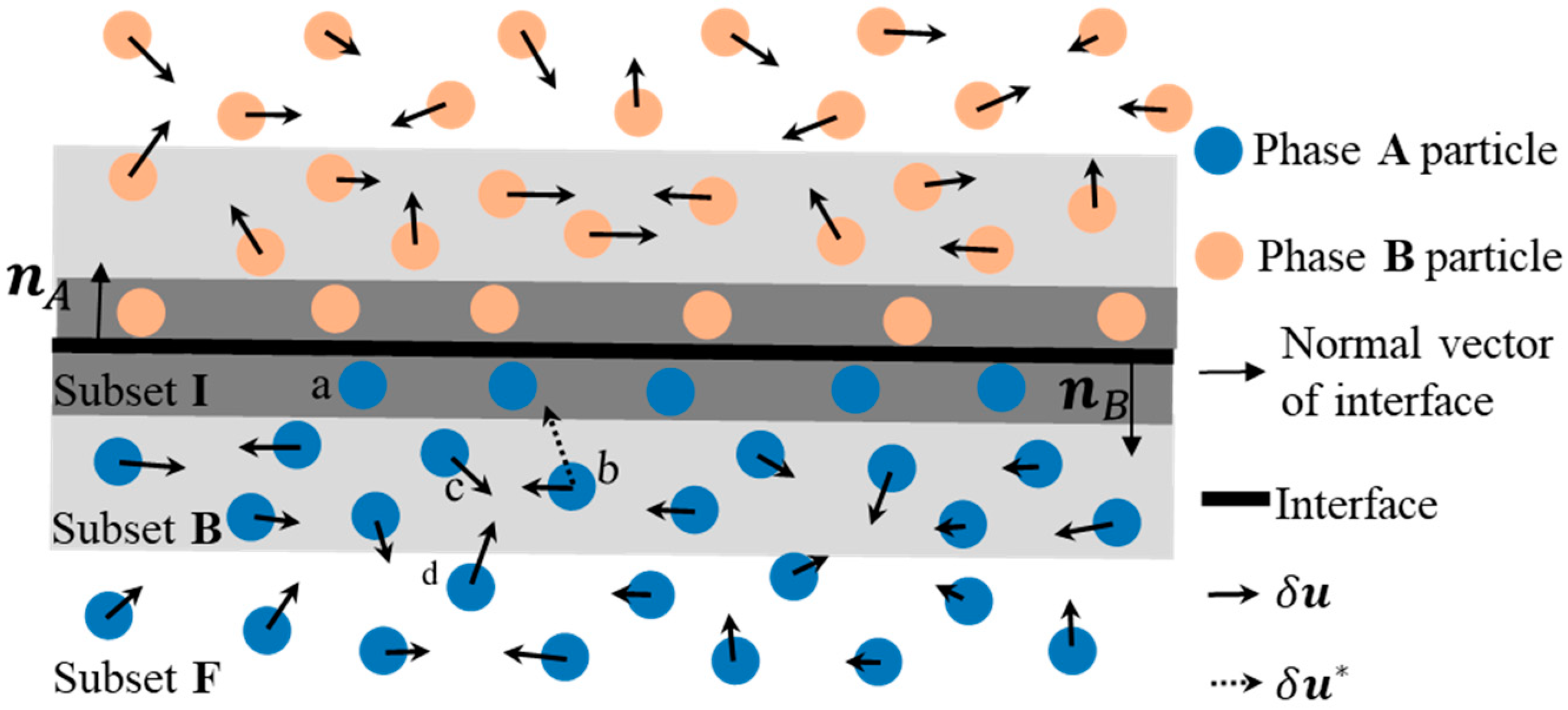
Special treatment is required to prevent artificial mixing of the different phase particles. For the particle belonging to the phase interfaces or domain boundaries, $\delta \mathit{u}$ is set to 0, as with particle a in Figure 2. For the particle in the vicinity of the phase interfaces or domain boundaries, $\delta \mathit{u}$ is set to be parallel to the phase interface of the domain boundaries when $\delta {\mathit{u}}^{*}$ drives the particle to move toward another phase, as with particle b in Figure 2. For other particles, no correction is needed, as with particles b and c in Figure 2. The correction method developed in the present work can be expressed as:

$$\delta {\mathit{u}}_i=\{\begin{array}{c}0 if i\in S_I\\ \left(\mathit{I}-{\mathit{n}}_i\otimes {\mathit{n}}_i\right)\delta {\mathit{u}}_i^{*} if i\in S_N \mathrm{and} \delta {\mathit{u}}_i^{*}·{\mathit{n}}_i\ge 0\\ \delta {\mathit{u}}_i^{*} if i\in S_N \mathrm{and} \delta {\mathit{u}}_i^{*}·{\mathit{n}}_i<0\\ \delta {\mathit{u}}_i^{*} if i\in S_F,\end{array}$$

(31)

where $S_I$ indicates the subset belonging to the phase interfaces or domain boundaries, $S_N$ is the subset in the vicinity of the phase interfaces or domain boundaries, $S_F$ is the subset of inner particles, and ${\mathit{n}}_i$ is the normal vector to the phase interfaces or domain boundaries of particle $i$.

The particle subsets are divided based on ${\lambda }_i$, which is the minimum eigenvalue of tensor ${\mathit{B}}_i=\left[{{\displaystyle \sum }}_{j\in \chi }\left({\mathit{r}}_j-{\mathit{r}}_i\right)⨂{\nabla }_i{W}_{ij}{V}_j\right]$. In the present work, if ${\lambda }_i<0.55$, particle $i$ belongs to $S_I$; if $0.55\le {\lambda }_i\le 0.90$, particle $i$ belongs to $S_N$; if ${\lambda }_i>0.90$, particle $i$ belongs to $S_F$. The normal vector to the phase interfaces or domain boundaries of particle $i$ is defined as:

$$\{\begin{array}{c}{\mathit{n}}_i=\frac{{\langle \nabla \lambda \rangle }_i}{\Vert {\langle \nabla \lambda \rangle }_i\Vert }\\ {\langle \nabla \lambda \rangle }_{\mathit{i}}=-{{\displaystyle \sum }}_{j\in \chi }\left({\lambda }_j-{\lambda }_i\right){\mathit{L}}_i{\nabla }_i{W}_{ij}{V}_j.\end{array}$$

(32)

Figure 2. Shifting treatment near the phase interface.

Figure 2. Shifting treatment near the phase interface.

3.4. Boundary Condition

Different boundary treatments have been developed to model the boundary surface. The fixed ghost particle technique [45] is adopted here to model the boundary surface. In this technique, the solid boundaries are discretized by fixed ghost particles. For each fixed ghost particle, there is a corresponding interpolation particle located in the fluid domain (see ghost particle $a$ and interpolation particle $a^{\prime }$ in Figure 3). The physical quantities of the interpolation particles are calculated by moving least-squares interpolation.

The pressure of the ghost particle is calculated as follows to avoid the unphysical penetration of the fluid particles:

$$P_G={{\displaystyle \sum }}_{j\in \mathrm{Fluid}}{P}_j{W}^{MLS}\left({\mathit{r}}_j\right)V_j+2d{\rho }_f\mathit{n}·\mathit{g},$$

(33)

where $d$ denotes the distance between the ghost particle and boundary surface, $\mathit{n}$ is the normal vector to the boundary surface, ${\rho }_f$ is the reference density of the denser fluid, and $W^{MLS}$ is the moving least-squares kernel, which can be expressed as:

$$\{\begin{array}{c}{W}^{MLS}\left({\mathit{r}}_j\right)={\mathit{M}}_i^{-1}{\mathit{e}}_1·{\mathit{b}}_{ij}W\left({\mathit{r}}_j\right)\\ {\mathit{M}}_i={{\displaystyle \sum }}_{j\in \mathrm{Fluid}}{\mathit{b}}_{ij}⨂{\mathit{b}}_{ij}W\left({\mathit{r}}_j\right)V_j\\ {\mathit{b}}_{ij}^T=\left[1,\left(x_j-x_i\right),\left(y_j-y_i\right)\right]\\ {\mathit{e}}_1^T=\left[1,0,0\right].\end{array}$$

(34)

The no-slip condition is implemented by setting the velocity of the fixed ghost particle as:

$${\mathit{u}}_G=-{{\displaystyle \sum }}_{j\in \mathrm{Fluid}}{\mathit{u}}_j{W}^{MLS}\left({\mathit{r}}_j\right)V_j.$$

(35)

For multiphase flows, it is important to predict the dynamic viscosity near the boundary to solve the viscous term in Equation (3). The viscous force provided by the boundary force is calculated based on Equation (24). The viscosity of ghost particle ${\mu }_G$ plays a key role in calculating the viscous force provided by the boundary surface. The viscosity of ghost particle ${\mu }_G$ is calculated based on the rheological model of the different phase. The value of ${\mathit{M}}_{11}$ is used to determine the rheological model of the ghost particle. As shown in Figure 3, the value of ${\mathit{M}}_{11}$ can be divided into the contribution of phases ${\mathit{M}}_{11}^A$ and ${\mathit{M}}_{11}^B$. If ${\mathit{M}}_{11}^A>{\mathit{M}}_{11}^B$, then the viscosity of ghost particle ${\mu }_G$ is calculated based on the rheological model of phase A, as shown for particle a in Figure 3; if ${\mathit{M}}_{11}^B>{\mathit{M}}_{11}^A$, then the viscosity of ghost particle ${\mu }_G$ is calculated based on the rheological model of phase B, as shown for particle b in Figure 3.

3.5. Time-Step Scheme

The fourth-order Runge–Kutta integration scheme is used to integrate SPH equations. The time step $\Delta t$ is restricted by the maximum velocity and maximum viscosity. The time-step constraints are expressed as [46]:

$$\Delta t=\min \left(\Delta t_c,\Delta t_d\right),$$

(36)

$$\Delta t_c\le {\alpha }_c\frac{h}{U_{max}},$$

(37)

$$\Delta t_d\le {\alpha }_d\frac{h^2{\rho }_{min}}{{\mu }_{max}},$$

(38)

where ${\alpha }_c$ and ${\alpha }_d$ are constants with an order of 0.1.

4. GPU Implementation

Particle-based methods are often criticized for their high calculation costs [47,48]. Different parallel computing architectures such as MPI [28], OpenMP [49], OpenCL [50], and CUDA [51] are commonly used to alleviate this drawback. Among these parallel computing architectures, CUDA is the most popular framework that can take advantage of the GPU’s computational horsepower. In the present work, we develop a CUDA-based parallel implementation on GPU architecture of the multiphase δ-plus-SPH model. As shown in Figure 4, the model can be split into four main steps: (1) building neighbor lists; (2) computing the physical quantities of ghost particles and the auxiliary variables of fluid particles; (3) solving the momentum and continuity equations; (4) and updating the physical quantities of the fluid particles.

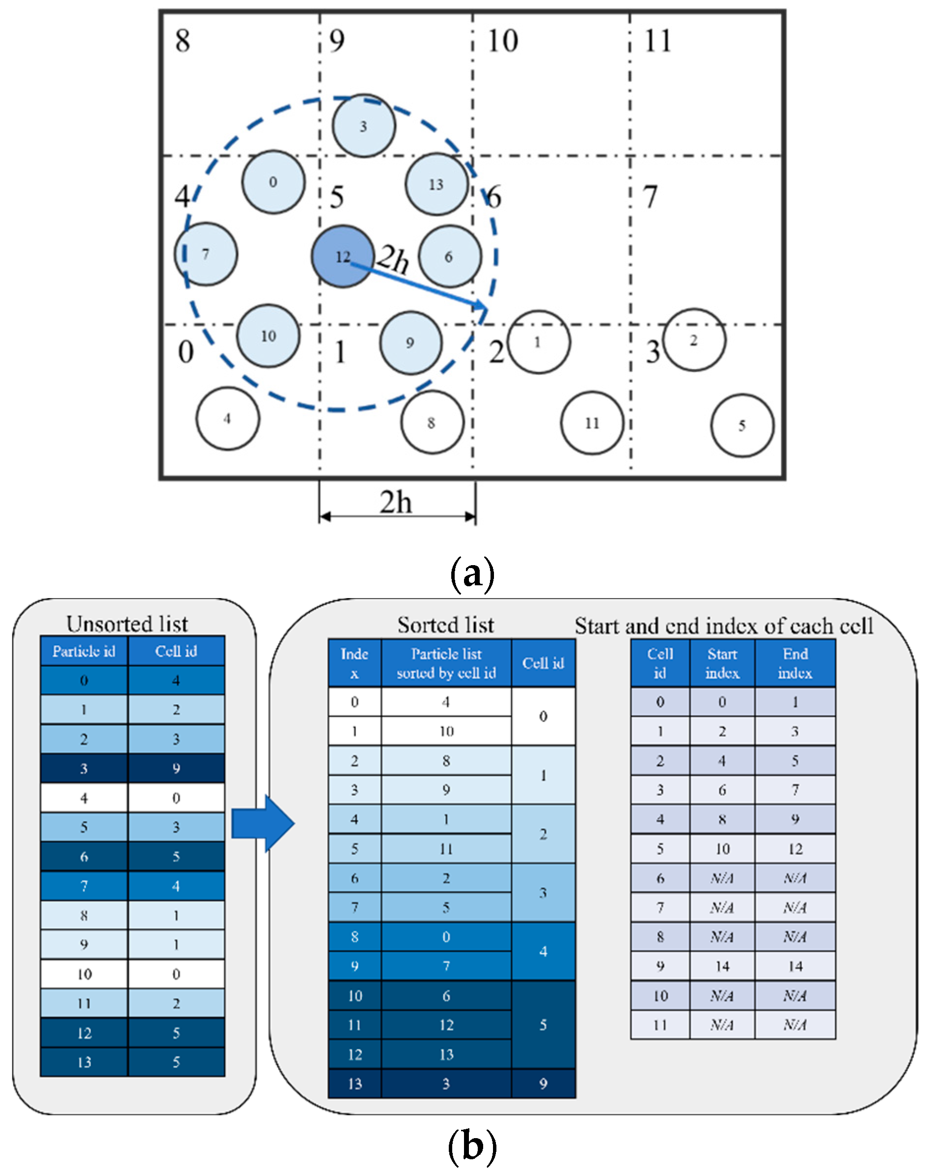
Among these four main steps, the nearest-neighbor search subroutine is considered to be the core of SPH [52]. Different nearest-neighbor search algorithms have been proposed to reduce the run time and memory consumption [53,54]. The modified linked list proposed by Green [55] is adopted in the present work. Similar to the cell-linked list method [56], the computational domain is divided into 2 h × 2 h cells. As shown in Figure 5a, a particle must only search its own cell and surrounding cells for possible particle interactions. To build the linked list, each particle is assigned to the corresponding cell, as shown in Figure 5b. However, this unsorted list is properly grouped in memory and it is hard to locate neighbor particles based on the cell ID. In the present work, the particles are sorted based on the cell ID, as shown in Figure 5b. The list of the starting and ending indexes of each cell ID is also built to make the sorted list useful. Based on these two lists, one can easily find the neighbor particles of any particle.

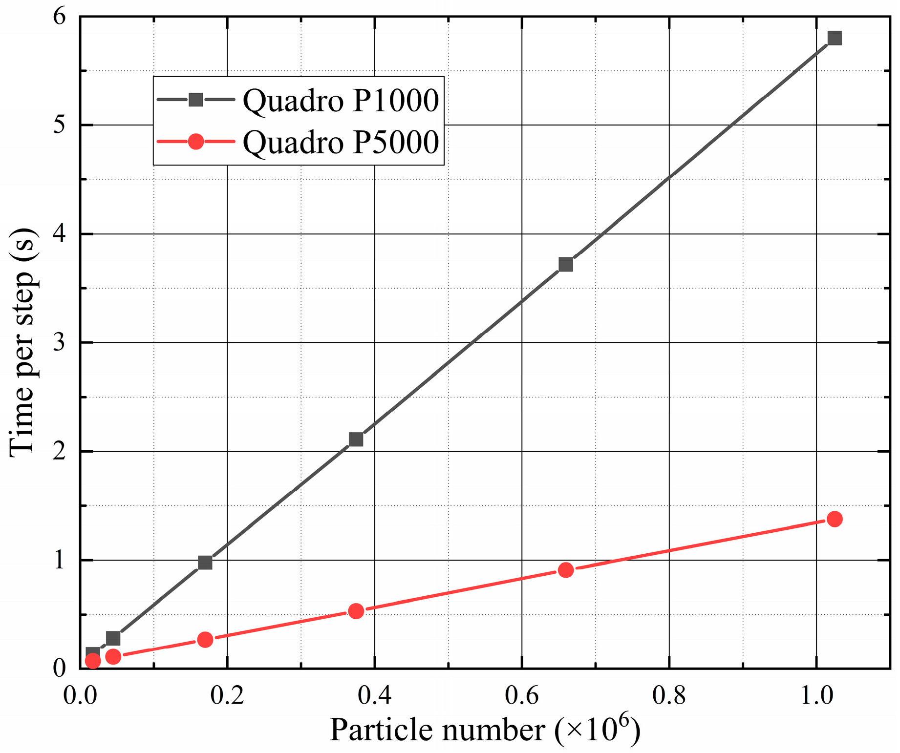
The performance of the GPU implementation was evaluated by increasing the spatial resolution of the static tank case (See Section 5.1 for details). Each case was run on two GPU cards, namely an Nvidia Quadro P1000 and Nvidia Quadro P5000. The relationships between calculation time per step and particle number are described in Figure 6. It shows that the calculation time per step increased linearly with the particle number. The ratio of the scalability (defined as the slope of the line) between the Quadro P1000 and Quadro P5000 was 4.33 for calculation time per step.

5. Numerical Results

5.1. Static Tank

A static tank is commonly applied to validate the efficiency of the boundary conditions and long-time hydrostatic pressure. Here, we conducted a static test to show that our model can remove the high-frequency pressure noise in the multiphase WCSPH model.

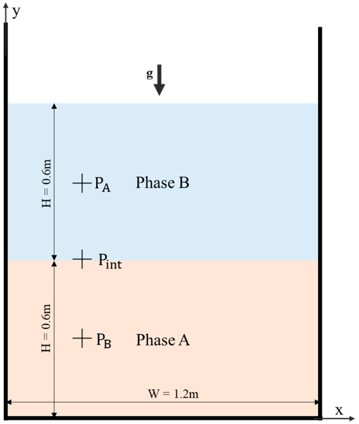
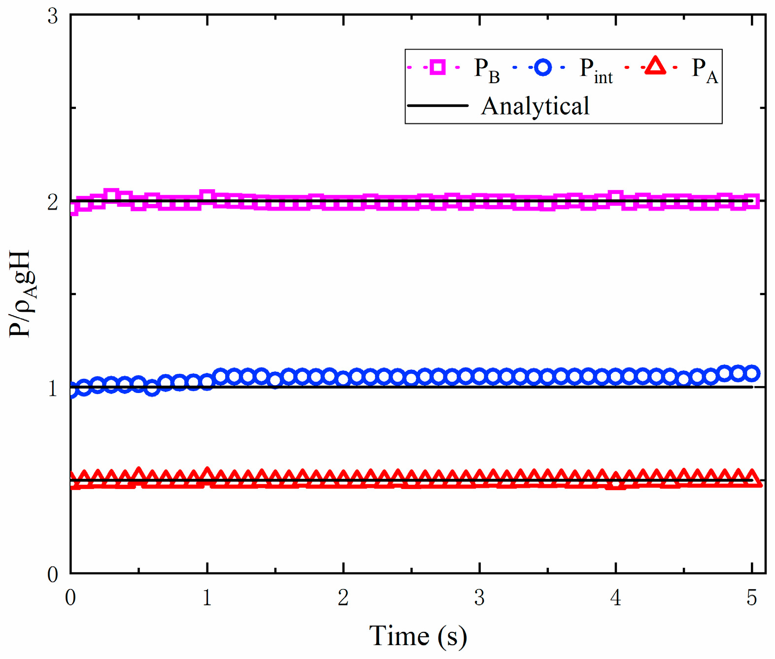
We considered a 2D 1.2 m × 1.5 m static tank, as presented in Figure 7. The static tank contained two horizontal layers of fluid. The height of each layer was 0.6 m. Three pressure monitor probes $P_A \left(0.3,0.9\right)$, $P_{int} \left(0.3,0.6\right)$, and $P_B \left(0.3,0.3\right)$ were arranged to record the pressure evolution during the numerical simulation. The physical and rheological parameters of each phase are listed in

Table 1. Physical and rheological parameters used in static tank test.

Parameter	Phase A	Phase B
$\mathit{\rho }$(kg/m3)	2000	1000
${\mathit{\tau }}_{\mathit{y}}$(N/m2)	10	0
K (Pa∙sN)	100	0.001
N	0.8	1

. The gravitational acceleration g was set as (0, −9.8).

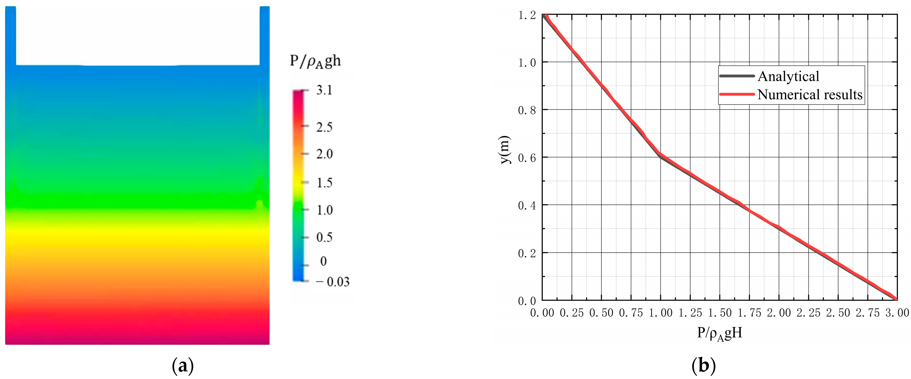
The pressure field of the static tank at t = 3.5 s is given in Figure 8a. The present pressure field obtained by the multiphase SPH model was smooth and continuous. Boundary particles could obtain proper pressure values via MLS interpolation. The pressure profile in the middle of the tank is presented in Figure 8b. In general, the numerical pressure profile was consistent with the analytical profile. There was a little deviation near the free surface owing to the backpressure used in the equation of state. Due to the SPH approximation feature, the evolution of numerical pressure near the phase interface was smoother than the evolution of the analytical pressure. The pressure history of the three monitor probes is presented in Figure 9. The results show that the numerical pressure values of each probe reached a steady state at 1 s. The numerical pressure of each probe thereafter agreed well with the analytical values.

5.2. Two-Phase Poiseuille Flow

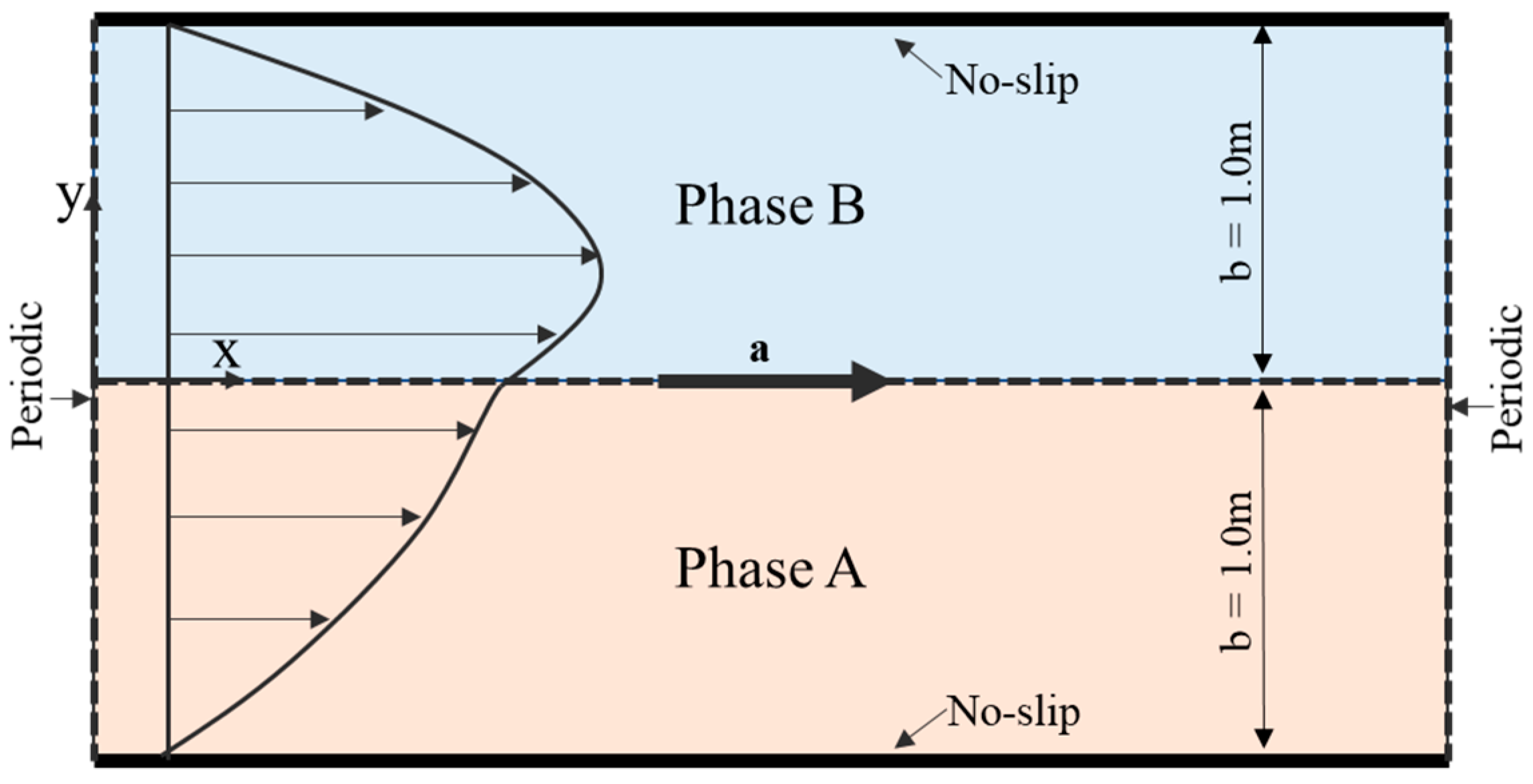
Poiseuille flows are used to validate the accuracy of the discretization scheme of the viscous term in a momentum equation. Two 1.0 m wide immiscible incompressible fluids were placed in the flow channel, as shown in Figure 10. The channel was limited by two fixed walls. No-slip boundaries were applied in the fixed walls. Periodic conditions were applied in the streamwise direction to produce a virtually infinitely large flow field. The fluids were driven by a constant body force $\Vert \mathit{a}\Vert =2.0\frac{\mathrm{m}}{{\mathrm{s}}^2}$. The density values of the two fluids were ${\rho }_A={\rho }_B=1.0\frac{\mathrm{kg}}{{\mathrm{m}}^3}$. Two test groups were investigated to simulate Newtonian/Newtonian interactions and Newtonian/non-Newtonian interactions.

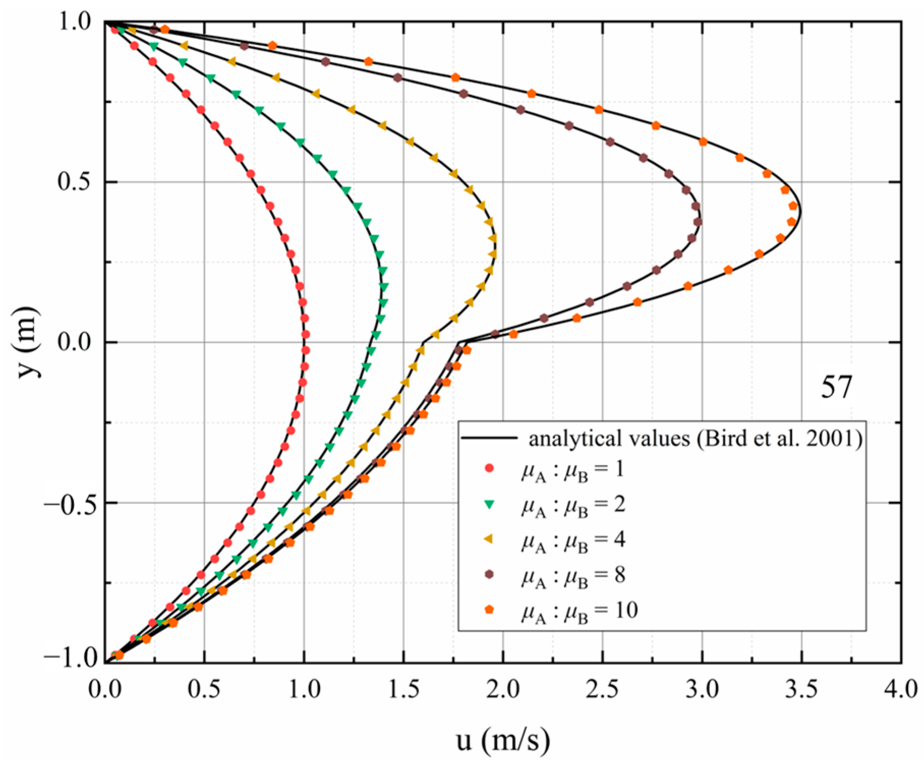
In the first test group, both phases were Newtonian fluids. The dynamic viscosity of phase A was set as ${\mu }_A$ = 1.0 Pa∙s. In the different test cases, the dynamic viscosity of phase B was varied from 1.0 to 0.1 Pa∙s. Bird et al. [57] proposed an analytical solution for the velocity profile of two Newtonian fluids in the steady state.

The calculated velocity profiles were compared with the analytical solutions in Figure 11. The velocity profiles of both phases formed a parabolic shape owing to the no-slip boundary condition applied at the fixed ghost particles (Figure 11). The velocity transition points of all test cases were located at the phase interface (Figure 11). Although the errors increased slightly with the increasing dynamic viscosity ratio between the two phases, there was still good agreement between the calculated velocity profiles and analytical velocity profiles.

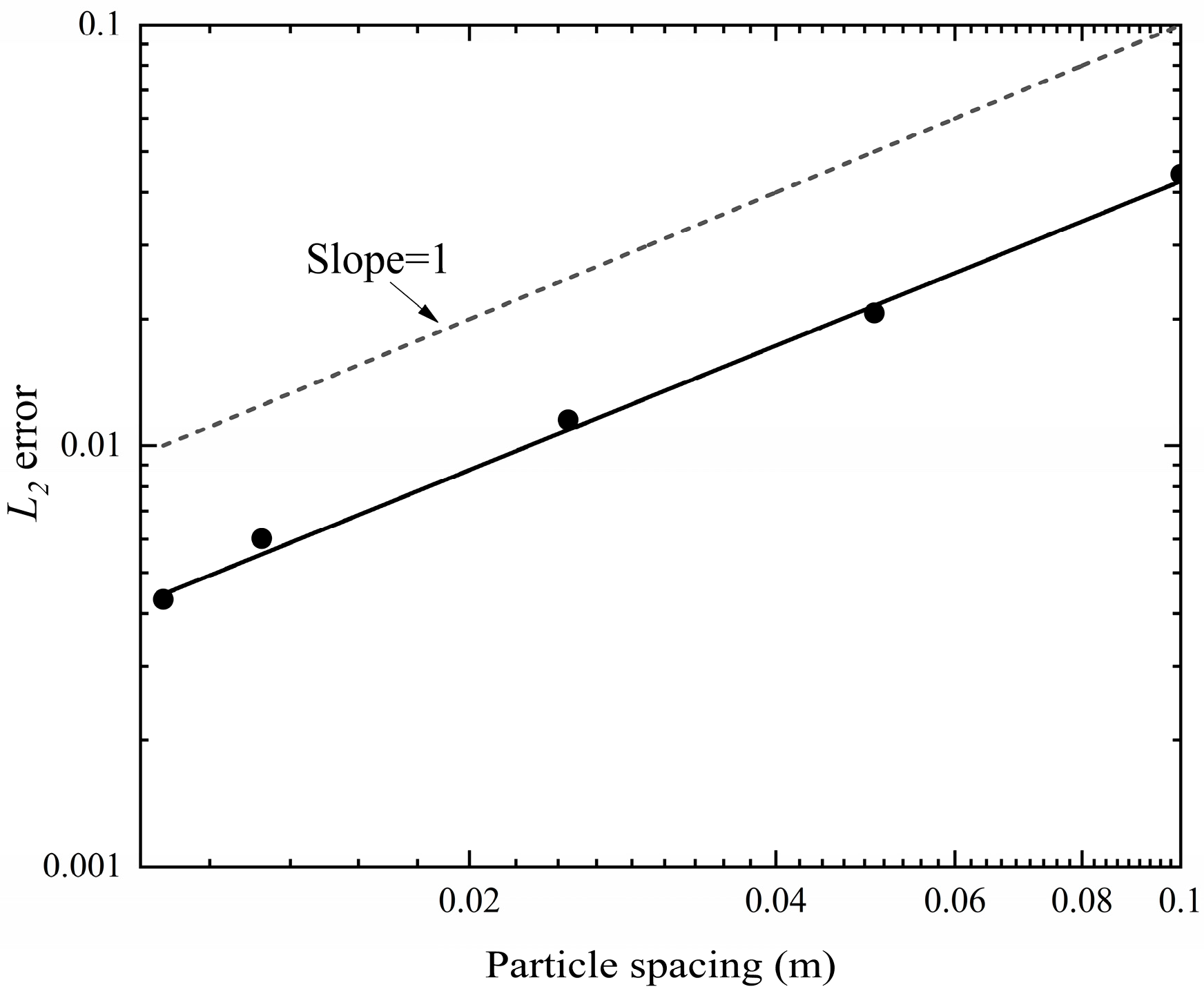
A convergence study was conducted for the case of ${\mu }_A:{\mu }_B=4$; the error can be expressed as:

$${ϵ}_{L2}=\sqrt{\frac{\sum {\left(u_{calculated}-u_{analytical}\right)}^2}{\sum u_{analytical}^2}}$$

(39)

As shown in Figure 12, the error decreased linearly with the particle spacing. The convergence rate of 1.0 indicates that the accuracy of the numerical solution improved at an expected rate with increasing spatial discretization.

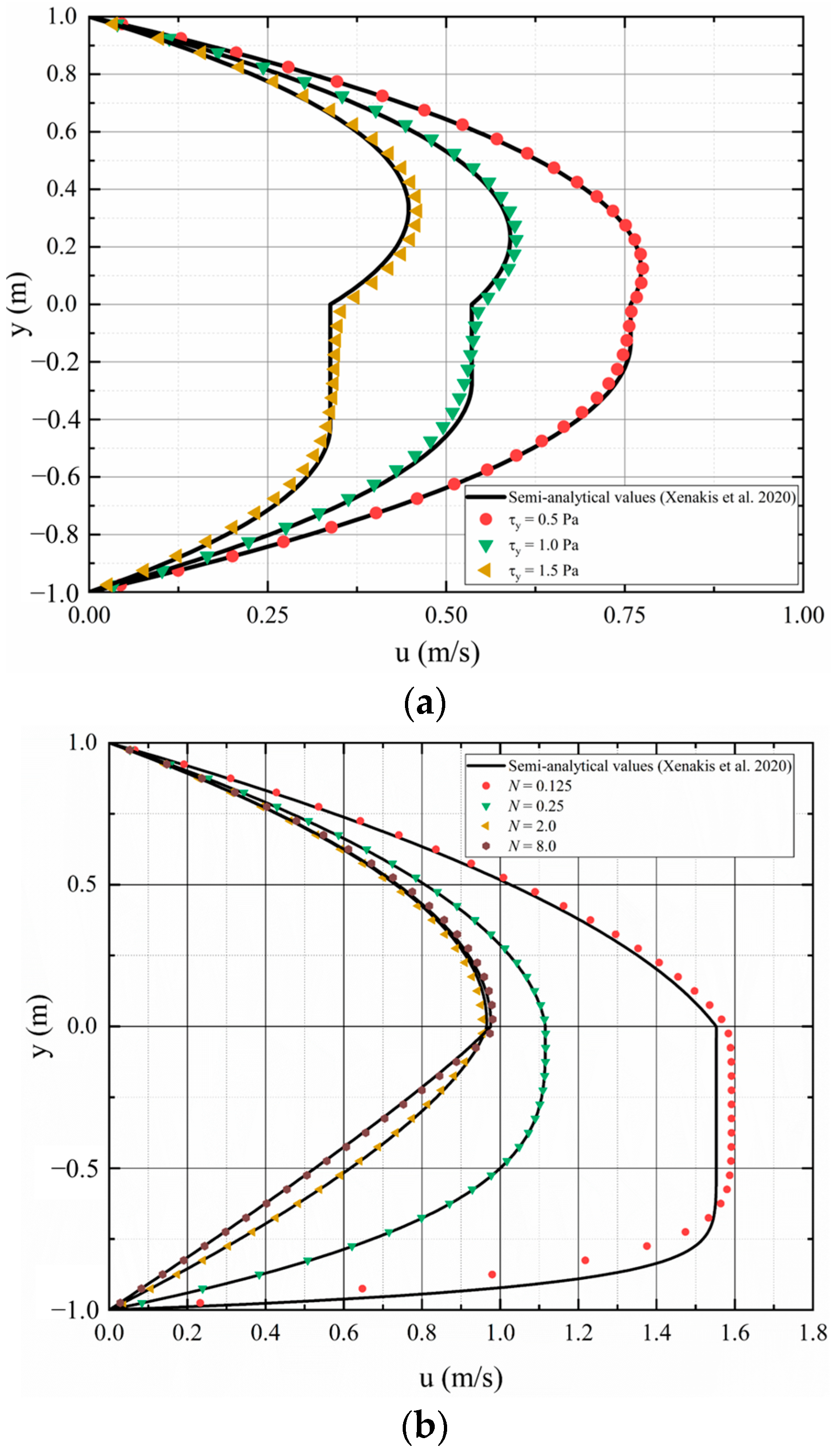
In the second test group, phase A was set as the non-Newtonian fluid and phase B was set as the Newtonian fluid. The dynamic viscosity of phase B ${\mu }_B$ remained 1.0 Pa∙s. For the non-Newtonian phase A, the parameters changed between different cases. K remained 1.0 Pa∙s^N in different cases. For the power law fluid cases, ${\tau }_y$ was equal to 0 and N varied from 0.125 to 8. For the Bingham fluid cases, N was equal to 1 and ${\tau }_y$ varied from 1 to 1.5 Pa. Xenakis et al. [16] proposed a semi-analytical solution for the steady state velocity profile of two-phase Newtonian/non-Newtonian Poiseuille flow.

A comparison between the calculated velocity profiles and semi-analytical solutions for Bingham/Newtonian fluid interactions is presented in Figure 13a. As a typical viscoplastic material, a Bingham fluid acts like a rigid body when the shear stress is below the yield stress ${\tau }_y$, but flows like a viscous flow when the shear stress surpasses the yield stress ${\tau }_y$. As shown in Figure 13a, the proposed model could rationally describe the transition from the yield zone to the non-yielding zone and the transition from the non-yielding zone to the Newtonian fluid zone. However, the errors increased with increasing yield stress ${\tau }_y$. This was because we set a relatively high “cut-off” shear rate value to maintain the numerical stability and obtain an acceptable time step. However, this relatively high “cut-off” shear rate results in a relatively low “cut-off” viscosity. The low “cut-off” viscosity causes the relatively soft non-yielding fluid.

A comparison between the calculated velocity profiles and semi-analytical solutions for the power law/Newtonian fluid interactions is presented in Figure 13b. The power-law model can describe the shear-thickening or shear-thinning behavior depending on the power index N. For this paper, the shear-thickening and shear-thinning fluids were calculated with N > 1 and N < 1. For N > 1 cases, the calculated velocity profiles were very close to the semi-analytical solutions. For N < 1 cases, this consistency decreased with decreasing N. This phenomenon can also be attributed to the relatively high “cut-off” shear rate value in the numerical simulations.

In general, the proposed model managed to describe both the non-Newtonian fluid behaviors and their interaction with the Newtonian fluid.

5.3. Submarine Debris Flow

Submarine debris flows are widely distributed in offshore and coastal areas and can generate tsunamis in coastal areas. Numerous experimental [58,59,60,61] and computational studies [58,62,63,64,65] have therefore been conducted to study their flow mechanisms and possible catastrophic consequences. Non-Newtonian fluids like those in the Herschel–Bulkley model are commonly used to describe viscoplastic debris flow [58,63]. Thus, they represent a good test case to assess the performance of the multiphase SPH model.

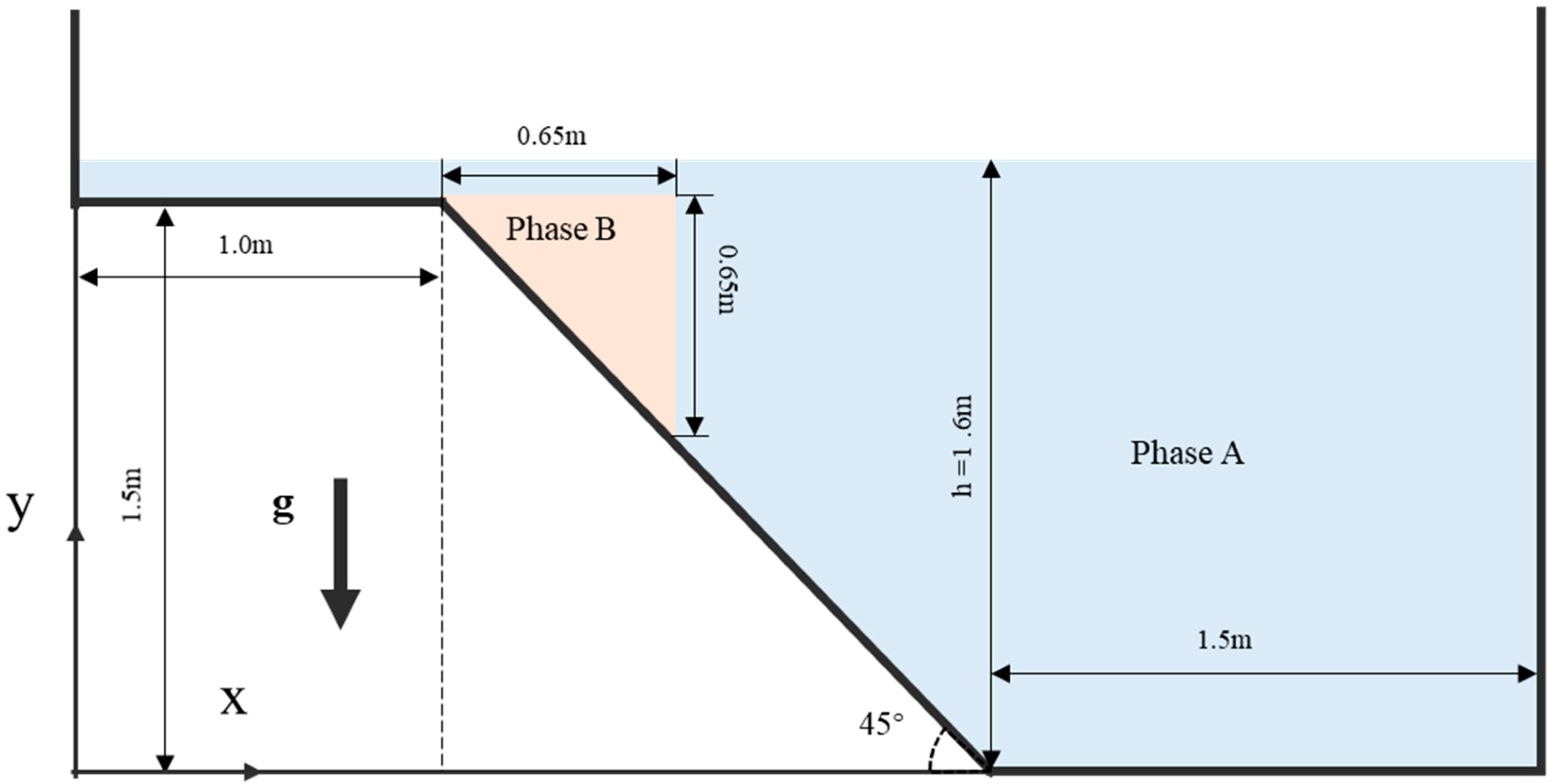
In the present work, the study conducted by Rzadkiewicz et al. [58] was simulated to examine the proposed multiphase SPH model. The geometrical configuration of the experimental setup is presented in Figure 14. The experiment was conducted in a 4 m × 2 m tank. Phase A was water and the maximum water depth was h = 1.6 m. Phase B was the mud mass, 0.65 m × 0.65 m in cross-section. The solid mass slid down along a slope of 45°. The rheological and physical parameters used in the simulation are presented in

Table 2. Physical and rheological parameters used in submarine debris flow test.

Parameter	Phase A	Phase B
$\mathit{\rho }$(kg/m3)	1000.0	1950.0
${\mathit{\tau }}_{\mathit{y}}$(N/m2)	0	1000.0
K (Pa∙sN)	0.001	1.0
N	1.0	1.0

. The rheological parameters of phase B were chosen based on the numerical tests conducted by Capone et al. [65].

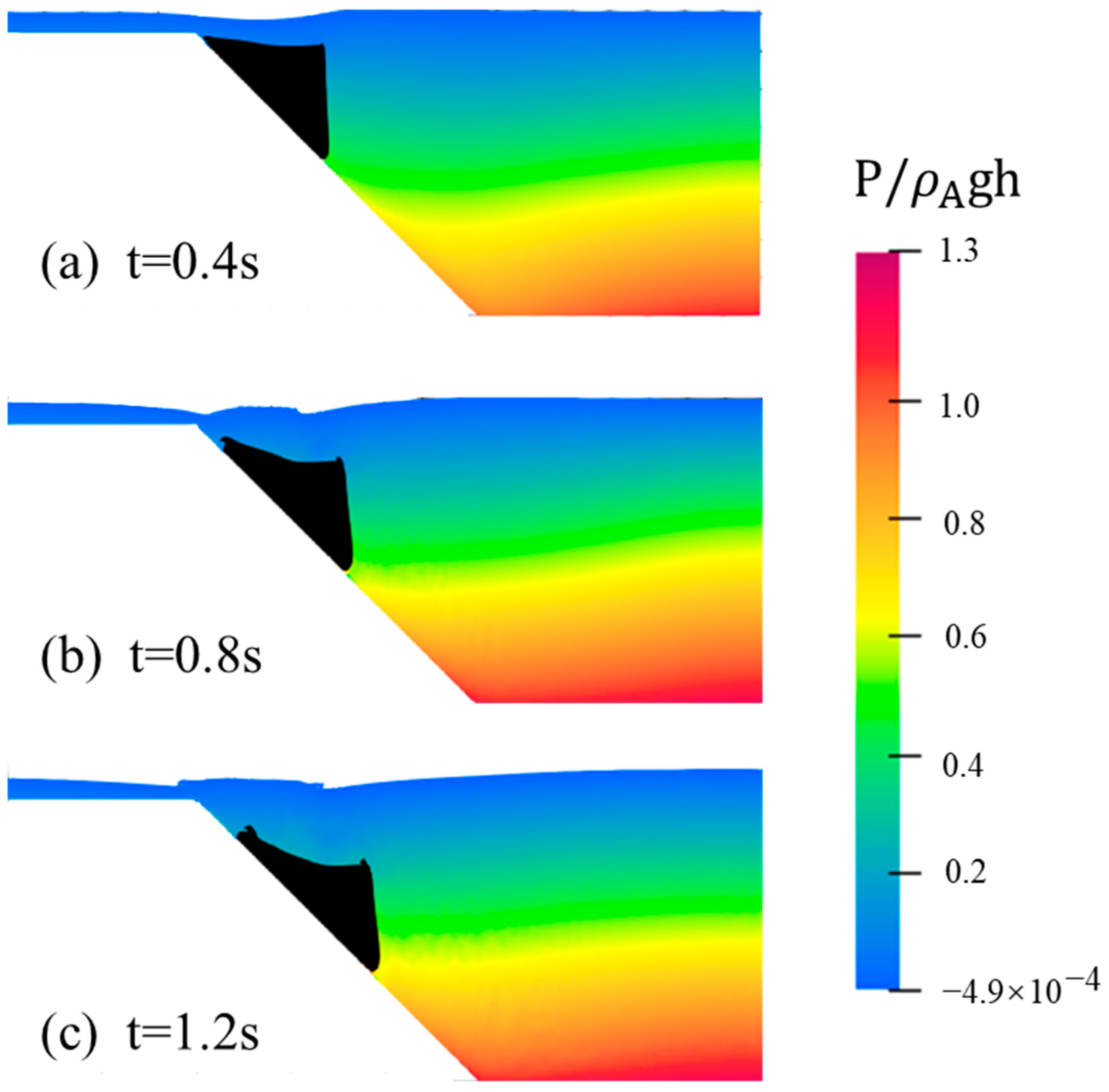
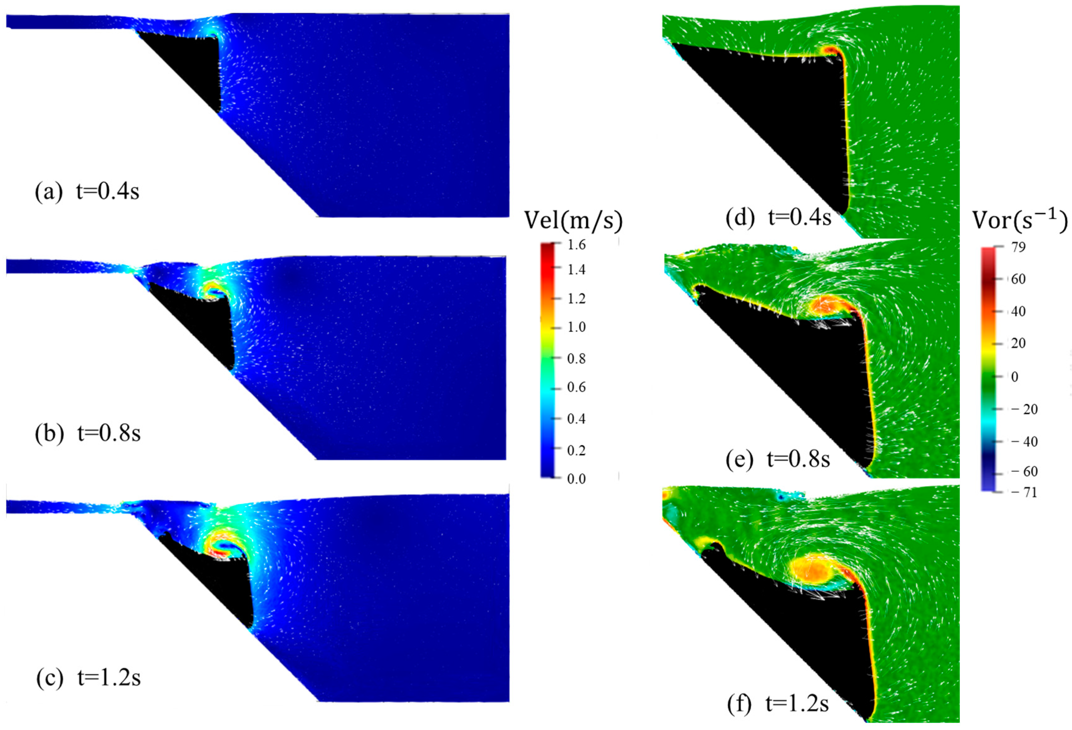
Figure 15 shows the calcuated values obtained by the proposed model at typical instants, where the particles of phase A are colored with their pressures. It can be observed that the pressure field of phase A is smooth and continuous. The evolution of the velocity and vorticity fields is presented in Figure 15, which describes the interaction between mud mass and water. After the mud mass was released, it accelerated under gravity. As shown in Figure 16a–c, surge waves were generated by the underwater mud mass flow. Figure 16d–f show that a shear layer formed between the interface and front of the mud mass and water, and a vortex was produced on the top of the mud mass as mud mass slid along the slope.

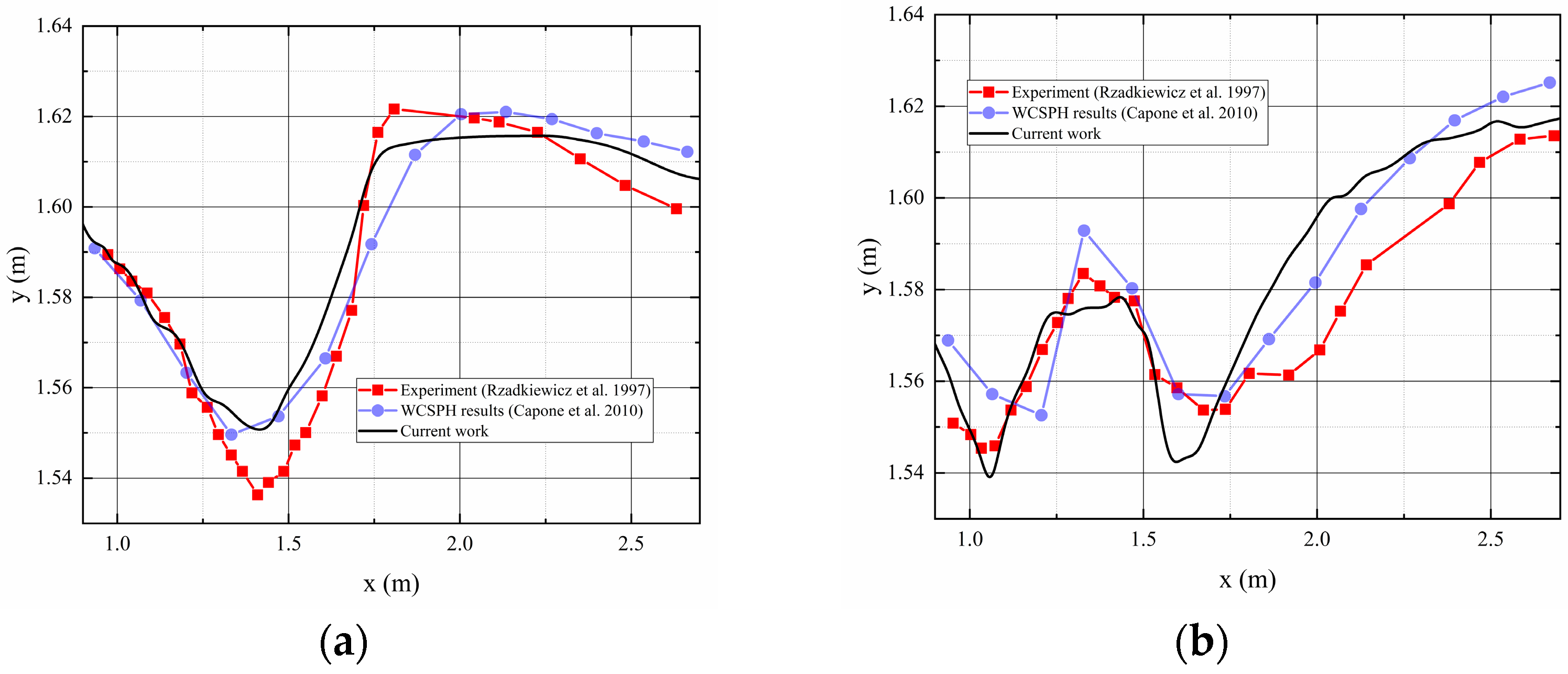
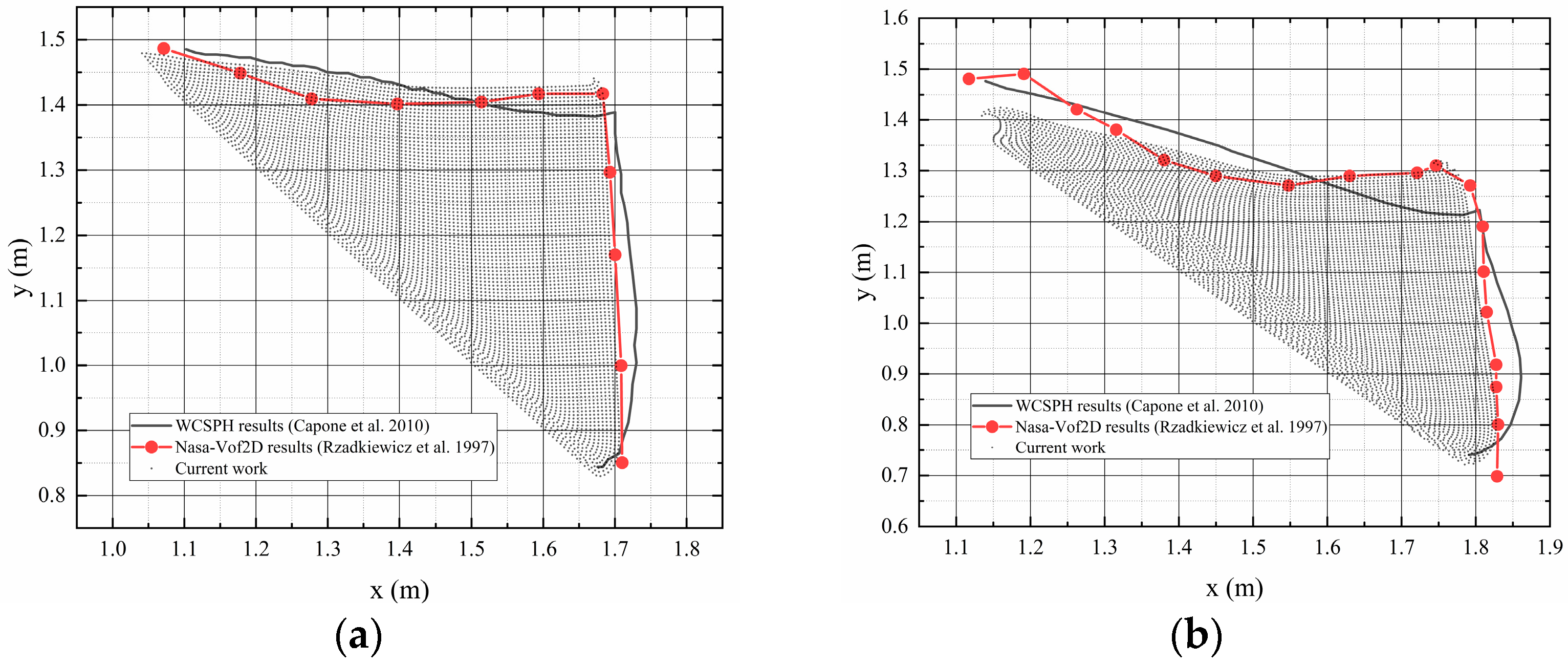
The generated surge wave profiles at t = 0.4 and 0.8 s were compared with the experimental data [58] and the WCSPH computational results [65]. The generated surge wave profile was found to be in accordance with the experimental data at t = 0.4 s, as shown in Figure 17b. The calculated profile could reflect the experimental data well when x < 1.5 m. However, similar to the results obtained by Capone et al. [65], the proposed method overpredicted the free-surface profile when x > 1.8 m. Comparisons were also made for mud mass between the results from the current work, the Nasa-Vof2D computational results [58], and the WCSPH computational results [65], as shown as Figure 18. The configurations of mud mass obtained in the current work were in good agreement with the Nasa-Vof2D computational results [58].

6. Conclusions

Non-Newtonian multiphase flows are widely found in many fields and have traditionally been considered to be a challenging topic due to the sharp material discontinuities and complex interface. This paper presents an extension of the δ-plus-SPH model for solving multiphase flows.

Two major improvements are proposed in this paper. First, the modified numerical diffusive term and special shifting treatment near the phase interface are developed and implemented in the original δ-plus-SPH model. These modifications allow the δ-plus-SPH model to describe multiphase flow. Secondly, the GPU-based parallel δ-plus-SPH model is implemented in CUDA and C++ to improve its computational efficiency in this paper.

After a detailed description of the proposed multiphase SPH model, three typical numerical test cases are provided to assess the performance of the new multiphase SPH model. Good agreements are found in the comparison with analytical solutions, numerical results, and the experimental data available in the literature. It can be concluded that the improved δ-plus-SPH model can provide more accurate and stable solutions for highly transient incompressible two-phase flows.

References

- Ouda, M.; Toorman, E.A. Development of a new multiphase sediment transport model for free surface flows. Int. J. Multiph. Flow 2019, 117, 81–102. [Google Scholar] [CrossRef]
- Ratkovich, N.; Majumder, S.K.; Bentzen, T.R. Empirical correlations and CFD simulations of vertical two-phase gas-liquid (Newtonian and non-Newtonian) slug flow compared against experimental data of void fraction. Chem. Eng. Res. Des. 2013, 91, 988–998. [Google Scholar] [CrossRef]
- Biscarini, C. Computational fluid dynamics modelling of landslide generated water waves. Landslides 2010, 7, 117–124. [Google Scholar] [CrossRef]
- Hao, Y.; Prosperetti, A. A numerical method for three-dimensional gas-liquid flow computations. J. Comput. Phys. 2004, 196, 126–144. [Google Scholar] [CrossRef]
- Dias, F.; Dutykh, D.; Ghidaglia, J.M. A two-fluid model for violent aerated flows. Comput. Fluids 2010, 39, 283–293. [Google Scholar] [CrossRef] [Green Version]
- Hirt, C.; Nichols, B. Volume of fluid (VOF) method for the dynamics of free boundaries. J. Comput. Phys. 1981, 39, 201–225. [Google Scholar] [CrossRef]
- Gu, H.B.; Causon, D.M.; Mingham, C.G.; Qian, L. Development of a free surface flow solver for the simulation of wave/body interactions. Eur. J. Mech. B Fluids 2013, 38, 1–17. [Google Scholar] [CrossRef]
- Yang, J.; Jeong, D.; Kim, J. A fast and practical adaptive finite difference method for the conservative Allen–Cahn model in two-phase flow system. Int. J. Multiph. Flow 2021, 137, 103561. [Google Scholar] [CrossRef]
- Garoosi, F.; Hooman, K. Numerical simulation of multiphase flows using an enhanced Volume-of-Fluid (VOF) method. Int. J. Mech. Sci. 2022, 215, 106956. [Google Scholar] [CrossRef]
- Colagrossi, A.; Landrini, M. Numerical simulation of interfacial flows by smoothed particle hydrodynamics. J. Comput. Phys. 2003, 191, 448–475. [Google Scholar] [CrossRef]
- Hu, X.Y.; Adams, N.A. A multi-phase SPH method for macroscopic and mesoscopic flows. J. Comput. Phys. 2006, 213, 844–861. [Google Scholar] [CrossRef]
- Hammani, I.; Marrone, S.; Colagrossi, A.; Oger, G.; Le Touzé, D. Detailed study on the extension of the δ-SPH model to multi-phase flow. Comput. Methods Appl. Mech. Eng. 2020, 368, 113189. [Google Scholar] [CrossRef]
- Grenier, N.; Antuono, M.; Colagrossi, A.; Le Touzé, D.; Alessandrini, B. An Hamiltonian interface SPH formulation for multi-fluid and free surface flows. J. Comput. Phys. 2009, 228, 8380–8393. [Google Scholar] [CrossRef]
- Chen, Z.; Zong, Z.; Liu, M.B.; Zou, L.; Li, H.T.; Shu, C. An SPH model for multiphase flows with complex interfaces and large density differences. J. Comput. Phys. 2015, 283, 169–188. [Google Scholar] [CrossRef]
- Zainali, A.; Tofighi, N.; Shadloo, M.S.; Yildiz, M. Numerical investigation of Newtonian and non-Newtonian multiphase flows using ISPH method. Comput. Methods Appl. Mech. Eng. 2013, 254, 99–113. [Google Scholar] [CrossRef]
- Xenakis, A.M.; Lind, S.J.; Stansby, P.K.; Rogers, B.D. An incompressible smoothed particle hydrodynamics scheme for Newtonian/non-Newtonian multiphase flows including semi-analytical solutions for two-phase inelastic Poiseuille flows. Int. J. Numer. Methods Fluids 2020, 92, 703–726. [Google Scholar] [CrossRef]
- Antuono, M.; Colagrossi, A.; Marrone, S.; Molteni, D. Free-surface flows solved by means of SPH schemes with numerical diffusive terms. Comput. Phys. Commun. 2010, 181, 532–549. [Google Scholar] [CrossRef]
- Antuono, M.; Colagrossi, A.; Marrone, S. Numerical diffusive terms in weakly-compressible SPH schemes. Comput. Phys. Commun. 2012, 183, 2570–2580. [Google Scholar] [CrossRef]
- Antuono, M.; Bouscasse, B.; Colagrossi, A.; Marrone, S. A measure of spatial disorder in particle methods. Comput. Phys. Commun. 2014, 185, 2609–2621. [Google Scholar] [CrossRef]
- Wang, P.P.; Meng, Z.F.; Zhang, A.M.; Ming, F.R.; Sun, P.N. Improved particle shifting technology and optimized free-surface detection method for free-surface flows in smoothed particle hydrodynamics. Comput. Methods Appl. Mech. Eng. 2019, 357, 112580. [Google Scholar] [CrossRef]
- Sun, P.N.; Colagrossi, A.; Marrone, S.; Zhang, A.M. The δplus-SPH model: Simple procedures for a further improvement of the SPH scheme. Comput. Methods Appl. Mech. Eng. 2017, 315, 25–49. [Google Scholar] [CrossRef]
- Sun, P.N.; Colagrossi, A.; Marrone, S.; Antuono, M.; Zhang, A.M. A consistent approach to particle shifting in the δ-Plus-SPH model. Comput. Methods Appl. Mech. Eng. 2019, 348, 912–934. [Google Scholar] [CrossRef]
- Wang, Z.B.; Chen, R.; Wang, H.; Liao, Q.; Zhu, X.; Li, S.Z. An overview of smoothed particle hydrodynamics for simulating multiphase flow. Appl. Math. Model. 2016, 40, 9625–9655. [Google Scholar] [CrossRef]
- Song, Y.; Huang, D.; Zeng, B. GPU-based parallel computation for discontinuous deformation analysis (DDA) method and its application to modelling earthquake-induced landslide. Comput. Geotech. 2017, 86, 80–94. [Google Scholar] [CrossRef]
- Zhang, A.; Sun, P.; Ming, F. An SPH modeling of bubble rising and coalescing in three dimensions. Comput. Methods Appl. Mech. Eng. 2015, 294, 189–209. [Google Scholar] [CrossRef]
- Wu, Y.; Tian, L.; Rubinato, M.; Gu, S.; Yu, T.; Xu, Z.; Cao, P.; Wang, X.; Zhao, Q. A new parallel framework of SPH-SWE for dam break simulation based on OpenMP. Water 2020, 50, 1395. [Google Scholar] [CrossRef]
- Oger, G.; Le Touzé, D.; Guibert, D.; De Leffe, M.; Biddiscombe, J.; Soumagne, J.; Piccinali, J.G. On distributed memory MPI-based parallelization of SPH codes in massive HPC context. Comput. Phys. Commun. 2016, 200, 1–14. [Google Scholar] [CrossRef]
- Cui, X.; Habashi, W.G.; Casseau, V. MPI Parallelisation of 3D Multiphase Smoothed Particle Hydrodynamics. Int. J. Comut. Fluid Dyn. 2020, 34, 610–621. [Google Scholar] [CrossRef]
- Liu, M.B.; Liu, G.R. Smoothed particle hydrodynamics (SPH): An overview and recent developments. Arch. Comput. Methods Eng. 2010, 17, 25–76. [Google Scholar] [CrossRef] [Green Version]
- Yang, L.; Rakhsha, M.; Hu, W.; Negrut, D. A consistent multiphase flow model with a generalized particle shifting scheme resolved via incompressible SPH. J. Comput. Phys. 2022, 458, 111079. [Google Scholar] [CrossRef]
- Xu, R.; Stansby, P.; Laurence, D. Accuracy and stability in incompressible SPH (ISPH) based on the projection method and a new approach. J. Comput. Phys. 2009, 228, 6703–6725. [Google Scholar] [CrossRef]
- Lind, S.J.; Xu, R.; Stansby, P.K.; Rogers, B.D. Incompressible smoothed particle hydrodynamics for free-surface flows: A generalised diffusion-based algorithm for stability and validations for impulsive flows and propagating waves. J. Comput. Phys. 2012, 231, 1499–1523. [Google Scholar] [CrossRef]
- Antuono, M.; Marrone, S.; Di Mascio, A.; Colagrossi, A. Smoothed particle hydrodynamics method from a large eddy simulation perspective. Generalization to a quasi-Lagrangian model. Phys. Fluids 2021, 33, 015102. [Google Scholar] [CrossRef]
- Zhang, G.; Chen, J.; Qi, Y.; Li, J.; Xu, Q. Numerical simulation of landslide generated impulse waves using a δ+-LES-SPH model. Adv. Water Resour. 2021, 151, 103890. [Google Scholar] [CrossRef]
- Kaitna, R.; Rickenmann, D.; Schatzmann, M. Experimental study on rheologic behaviour of debris flow material. Acta Geotech. 2007, 2, 71–85. [Google Scholar] [CrossRef]
- Burger, J.; Haldenwang, R.; Alderman, N. Experimental database for non-Newtonian flow in four channel shapes. J. Hydraul. Res. 2010, 48, 363–370. [Google Scholar] [CrossRef]
- Vajravelu, K.; Sreenadh, S.; Devaki, P.; Prasad, K.V. Peristaltic Transport of a Herschel-Bulkley Fluid in an Elastic Tube. Heat Transf. Asian Res. 2015, 44, 585–598. [Google Scholar] [CrossRef]
- Guo, T.; Zhao, K.; Zhang, Z.; Gao, X.; Qi, X. Rheology Study on Low-Sugar Apple Jam by a New Nonlinear Regression Method of Herschel-Bulkley Model. J. Food Process. Preserv. 2017, 41, e12810. [Google Scholar] [CrossRef]
- Di Mascio, A.; Antuono, M.; Colagrossi, A.; Marrone, S. Smoothed particle hydrodynamics method from a large eddy simulation perspective. Phys. Fluids 2017, 29, 035102. [Google Scholar] [CrossRef]
- Gotoh, H.; Shao, S.; Memita, T. SPH-LES model for numerical investigation of wave interaction with partially immersed breakwater. Coast. Eng. J. 2004, 46, 39–63. [Google Scholar] [CrossRef]
- Molteni, D.; Colagrossi, A. A simple procedure to improve the pressure evaluation in hydrodynamic context using the SPH. Comput. Phys. Commun. 2009, 180, 861–872. [Google Scholar] [CrossRef]
- Qi, Y.; Chen, J.; Zhang, G.; Xu, Q.; Li, J. An improved multi-phase weakly-compressible SPH model for modeling various landslides. Powder Technol. 2022, 397, 117120. [Google Scholar] [CrossRef]
- Randles, P.W.; Libersky, L.D. Smoothed particle hydrodynamics: Some recent improvements and applications. Comput. Methods Appl. Mech. Eng. 1996, 139, 375–408. [Google Scholar] [CrossRef]
- Hu, X.Y.; Adams, N.A. An incompressible multi-phase SPH method. J. Comput. Phys. 2007, 227, 264–278. [Google Scholar] [CrossRef]
- Marrone, S.; Antuono, M.; Colagrossi, A.; Colicchio, G.; Le Touzé, D.; Graziani, G. δ-SPH model for simulating violent impact flows. Comput. Methods Appl. Mech. Eng. 2011, 200, 1526–1542. [Google Scholar] [CrossRef]
- Fan, X.J.; Tanner, R.I.; Zheng, R. Smoothed particle hydrodynamics simulation of non-Newtonian moulding flow. J. Nonnewton. Fluid Mech. 2010, 165, 219–226. [Google Scholar] [CrossRef]
- Vacondio, R.; Altomare, C.; De Leffe, M.; Hu, X.; Le Touzé, D.; Lind, S.; Marongiu, J.C.; Marrone, S.; Rogers, B.D.; Souto-Iglesias, A. Grand challenges for Smoothed Particle Hydrodynamics numerical schemes. Comput. Part. Mech. 2021, 8, 575–588. [Google Scholar] [CrossRef]
- Yashiro, S. Application of particle simulation methods to composite materials: A review. Adv. Compos. Mater. 2017, 26, 1–22. [Google Scholar] [CrossRef]
- Dai, Z.; Huang, Y.; Cheng, H.; Xu, Q. 3D numerical modeling using smoothed particle hydrodynamics of flow-like landslide propagation triggered by the 2008 Wenchuan earthquake. Eng. Geol. 2014, 180, 21–33. [Google Scholar] [CrossRef]
- Cercos-Pita, J.L. AQUAgpusph, a new free 3D SPH solver accelerated with OpenCL. Comput. Phys. Commun. 2015, 192, 295–312. [Google Scholar] [CrossRef]
- Crespo, A.J.C.; Domínguez, J.M.; Rogers, B.D.; Gómez-Gesteira, M.; Longshaw, S.; Canelas, R.; Vacondio, R.; Barreiro, A.; García-Feal, O. DualSPHysics: Open-source parallel CFD solver based on Smoothed Particle Hydrodynamics (SPH). Comput. Phys. Commun. 2015, 187, 204–216. [Google Scholar] [CrossRef]
- Zheng, D.; Wu, P.; Shang, W.; Cao, X. Nearest neighbor search algorithm based on multiple background grids for fluid simulation. J. Shanghai Univ. 2011, 15, 405–408. [Google Scholar] [CrossRef]
- Awile, O.; Büyükkeçeci, F.; Reboux, S.; Sbalzarini, I.F. Fast neighbor lists for adaptive-resolution particle simulations. Comput. Phys. Commun. 2012, 183, 1073–1081. [Google Scholar] [CrossRef]
- Viccione, G.; Bovolin, V.; Carratelli, E.P. Defining and optimizing algorithms for neighbouring particle identification in SPH fluid simulations. Int. J. Numer. Methods Fluids 2008, 58, 625–638. [Google Scholar] [CrossRef]
- Green, S. Particle Simulation using CUDA; NVIDIA Whitepaper; NVIDIA: Santa Clara, CA, USA, 2013; pp. 1–12. [Google Scholar]
- Chen, J.Y.; Lien, F.S.; Peng, C.; Yee, E. GPU-accelerated smoothed particle hydrodynamics modeling of granular flow. Powder Technol. 2020, 359, 94–106. [Google Scholar] [CrossRef]
- Byron Bird, R.; Stewart, W.E.; Lightfoot, E.N. Transport Phenomena, 2nd ed.; Anderson, W., Ed.; Wiley: Hoboken, NJ, USA, 2001; Volume 1, ISBN 0471410772. [Google Scholar]
- Rzadkiewicz, S.A.; Mariotti, C.; Heinrich, P. Numerical Simulation of Submarine Landslides and Their Hydraulic Effects. J. Waterw. Port Coastal Ocean Eng. 1997, 123, 149–157. [Google Scholar] [CrossRef]
- Zakeri, A.; Høeg, K.; Nadim, F. Submarine debris flow impact on pipelines—Part I: Experimental investigation. Coast. Eng. 2008, 55, 1209–1218. [Google Scholar] [CrossRef]
- Yin, M.; Rui, Y. Laboratory study on submarine debris flow. Mar. Georesources Geotechnol. 2018, 36, 950–958. [Google Scholar] [CrossRef] [Green Version]
- Takabatake, T.; Mäll, M.; Han, D.C.; Inagaki, N.; Kisizaki, D.; Esteban, M.; Shibayama, T. Physical modeling of tsunamis generated by subaerial, partially submerged, and submarine landslides. Coast. Eng. J. 2020, 62, 582–601. [Google Scholar] [CrossRef]
- Zakeri, A.; Høeg, K.; Nadim, F. Submarine debris flow impact on pipelines—Part II: Numerical analysis. Coast. Eng. 2009, 56, 1–10. [Google Scholar] [CrossRef]
- Ren, Z.; Zhao, X.; Liu, H. Numerical study of the landslide tsunami in the South China Sea using Herschel-Bulkley rheological theory. Phys. Fluids 2019, 31, 056601. [Google Scholar] [CrossRef]
- Chen, Y.; Zhang, L.; Wei, X.; Jiang, M.; Liao, C.; Kou, H. Simulation of runout behavior of submarine debris flows over regional natural terrain considering material softening. Mar. Georesources Geotechnol. 2021, 1–20. [Google Scholar] [CrossRef]
- Capone, T.; Panizzo, A.; Monaghan, J.J. SPH modelling of water waves generated by submarine landslides. J. Hydraul. Res. 2010, 48, 80–84. [Google Scholar] [CrossRef]
Figure 3.
Boundary treatment.
Figure 4.
Flow diagram of the SPH model implemented on a GPU.
Figure 5.
Neighbor particle search algorithm. (a) Cell division in 2D; (b) sorted neighbor list.
Figure 6.
The relationship between calculation time per step and particle number on different GPU cards.
Figure 7.
Initial setup of the static tank test.
Figure 8.
(a) Snapshot of the pressure field at t = 3.5 s; (b) pressure profile at t = 3.5 s.
Figure 9.
Pressure history of the three monitor probes PA, PB, and Pint.
Figure 10.
Configuration of two-phase Poiseuille flow test.
Figure 11.
Velocity profiles of two-phase Newtonian Poiseuille flow tests.
Figure 12.
Numerical solution convergence result for the multiphase δ-plus-SPH model.
Figure 13.
Velocity profiles of Newtonian and non-Newtonian interactions. (a) Bingham/Newtonian fluid interactions; (b) power law/Newtonian interactions.
Figure 14.
Geometrical configuration of a submarine debris flow. Modified from [58].
Figure 15.
Snapshots of the pressure field at typical instants. (a) pressure field at t = 0.4 s; (b) pressure field at t = 0.8 s; (c) pressure field at t = 1.2 s.
Figure 16.
Evolution of the velocity and vorticity fields at typical instants. (a) velocity field at t = 0.4 s; (b) velocity field at t = 0.8 s; (c) velocity field at t = 1.2 s; (d) vorticity field at t = 0.4 s; (e) vorticity field at t = 0.8 s; (f) vorticity field at t = 1.2 s.
Figure 17.
Comparison of surge wave profiles. (a) t = 0.4 s; (b) t = 0.8 s.
Figure 18.
Phase B comparison between results from the current work, WCSPH [65], and Nasa-Vof2D [58]. (a) t = 0.4 s; (b) t = 0.8 s.