
Machine Learning Algorithms for Biophysical Classification of Lithuanian Lakes Based on Remote Sensing Data


Institute of Geosciences, Vilnius University, M. K. Čiurlionio 21/27, LT-03101 Vilnius, Lithuania
*
Author to whom correspondence should be addressed.
Water 2022, 14(11), 1732; https://doi.org/10.3390/w14111732
Submission received: 29 April 2022
/
Revised: 24 May 2022
/
Accepted: 26 May 2022
/
Published: 28 May 2022
(This article belongs to the Special Issue Water Quality Modeling and Monitoring)
Abstract
:Inland waters are dynamic systems that are under pressure from anthropogenic activities, thus constant observation of these waters is essential. Remote sensing provides a great opportunity to have frequent observations of inland waters. The aim of this study was to create a data-driven model that uses a machine learning algorithm and Sentinel-2 data to classify lake observations into four biophysical classes: Clear, Moderate, Chla-dominated, and Turbid. We used biophysical variables such as water transparency, chlorophyll concentration, and suspended matter to define these classes. We tested six machine learning algorithms that use spectral features of lakes as input and chose random forest classifiers, which yielded the most accurate results. We applied our two-step model on 19,292 lake spectra for the years 2015–2020, from 226 lakes. The prevalent class in 67% of lakes was Clear, while 19% of lakes were likely affected by strong algal blooms (Chla-dominated class). The models created in this study can be applied to lakes in other regions where similar lake classes are found. Biophysical lake classification using Sentinel-2 MSI data can help to observe long-term and short-term changes in lakes, thus it can be a useful tool for water management experts and for the public.
1. Introduction
Inland waters serve many purposes including recreational, drinking, part of the carbon cycle [1], an important habitat for living organisms [2], and providing ecosystem services. In the face of the warming climate [3] inland water bodies need constant observation. In situ measurements cover a small part of water bodies in the world and even fewer have long-term datasets. Larger water bodies are often included in state monitoring programs and are observed several times a year; however, the long-term state of the smaller ones is not known. Remote sensing data can help to observe many more water bodies, and some satellites provide an opportunity to construct time-series of a few decades [4]. Nonetheless, the satellite data validation is preferably carried out using in situ spectral data that are even more limited spatially and temporally than routinely carried out water parameter measurements.
Remote sensing data have largely improved the observation of spatial features of water bodies, including the distribution of phytoplankton (through the proxy—common algal pigment—chlorophyll α (chla) concentration [5]), suspended matter [6], and coloured dissolved matter [7]. The optical complexity of inland waters caused by the combination of the aforementioned compounds may impede the retrieval of chla when simple algorithms like band ratio algorithms are used [8]. Thus, grouping water bodies with similar prevalent substances and creating parameter retrieval algorithms for groups of lakes yield better results [9]. In addition, grouping, clustering or classifying lakes is a common way to characterise separable lake water types. In the European Union the ecological status of water bodies is defined by five classes: Poor, Bad, Moderate, Good, and High. The status is assessed using several measurements a year carried out by regional Environmental Protection Agencies; however, most of the water bodies are not measured every year. The use of satellite spectral data could help to fill in these data gaps.
The success of using remote sensing data for observation of inland water bodies depends on the inherent features of the data and water bodies, and the methodology used. The uncertainties arise from low signals of water, the influence of atmosphere, and the algorithms chosen for water parameters retrieval. In some cases using certain band difference algorithms for chla retrieval may give better results than using band ratio algorithms [10]. The retrieved water parameters can be used to derive information about the state of a lake, such as the trophic state of a lake [5].
Spectral resolution of a satellite sensor may also determine its ability to retrieve certain water parameters. The Operational Land Imager onboard the Landsat 8 satellite was shown to capture the reflectance peaks related to phytoplankton poorly in comparison to the Sentinel-2 Multispectral Imager (MSI) [8]. The band configuration of Sentinel-2 MSI is good for estimation of chlorophyll α and hyperspectral missions are just slightly better [11]. Currently having two satellites in orbit provides an opportunity to observe the same object every 2–3 days. In addition, the Sentinel-2 mission will be extended with coming satellites in the future [12]. With this in mind, it is highly desirable to have robust algorithms that use Sentinel-2 data that could highly improve the monitoring of water bodies.
Different techniques can be used for grouping water bodies. Unsupervised clustering techniques were used to group inland and coastal waters to optical water types using in situ hyperspectral datasets and 13 distinct types were identified for inland waters [13]. However, with the present non-hyperspectral satellites it may be difficult to separate so many classes. A simpler method that includes five classes: Clear, Moderate, Turbid, Very Turbid, Brown, was developed in Estonia using the k-means clustering technique [14]. The optical properties such as diffuse attenuation coefficient and diffuse reflectance, and commonly measured parameters such as transparency, chla concentration, total suspended matter (SM) and yellow substances, were used to determine the five classes. The latter framework has been used for studying Estonian lakes, coastal Baltic Sea, Wadden Sea [15] and Latvian lakes [9]. Another optical water type representation, consisting of eight types was developed for Brazilian waters [16]. The characterization of optical water types highly depends on the diversity of a dataset, number of features, and the number of samples that could be distinguished as a separate type.
Water body classification can be used itself as a source of data [9] or can be further used for algorithm development for retrieval of water parameters. Simple band ratio algorithms are being replaced by more complex algorithms that can combine the information of several features (for example, derivatives from spectral data) and provide better results. Supervised learning algorithms can be used for classification and for parameter retrieval—regression techniques are used. For retrieval of chla concentration, algorithms based on support vector machine for regression [6], artificial neural networks [17,18], Cubist [19], and random forest [20] have been developed. The selection of an algorithm depends on the nature of the data and the application. As there is no universal algorithm and the simplest algorithm is preferred over a complex one, often several algorithms are tested to choose the best performing algorithm for a particular application [21,22] or a framework based on automatic model selection can be used [23].
In most cases in situ optical data are used in model development; however, as mentioned earlier, this type of data are not always available, but nonetheless data-driven algorithms that use only water parameter data and satellite data may also provide good results [19]. In the study based on Czech lakes, 11 different spectral indices were derived from Sentinel-2 data and fed into machine learning algorithms. The Normalized Difference Vegetation Index, red/blue band ratio, and red-edge band, B5, were the most important features for derivation of chla concentration data, and Normalized Water Difference Index 3, the red-edge band, B5, and Normalized Difference Water Index 11 were the most important features for total suspended solids determination in Czech lakes [19].
The aim of this study is to create a data-driven model that uses machine learning methods and satellite data as input to assign a biophysical class to a lake. The classes are defined by often routinely measured—according to monitoring programmes—water quality parameters, such as, chla concentration, water transparency, and SM. For model development we used data of 226 lakes in Lithuania. The classification of lake observations was implemented in two steps—at first using binary classification for separation of Clear class from lakes with optically active substances and then multi-class classification for differentiating lakes with significant amounts of optically active substances into three classes differentiated by turbidity and the dominant optically active substance. The created model could be used in areas where in situ spectral data are not available, which hinders the use of satellite data in these locations.
2. Materials and Methods
2.1. Study Objects
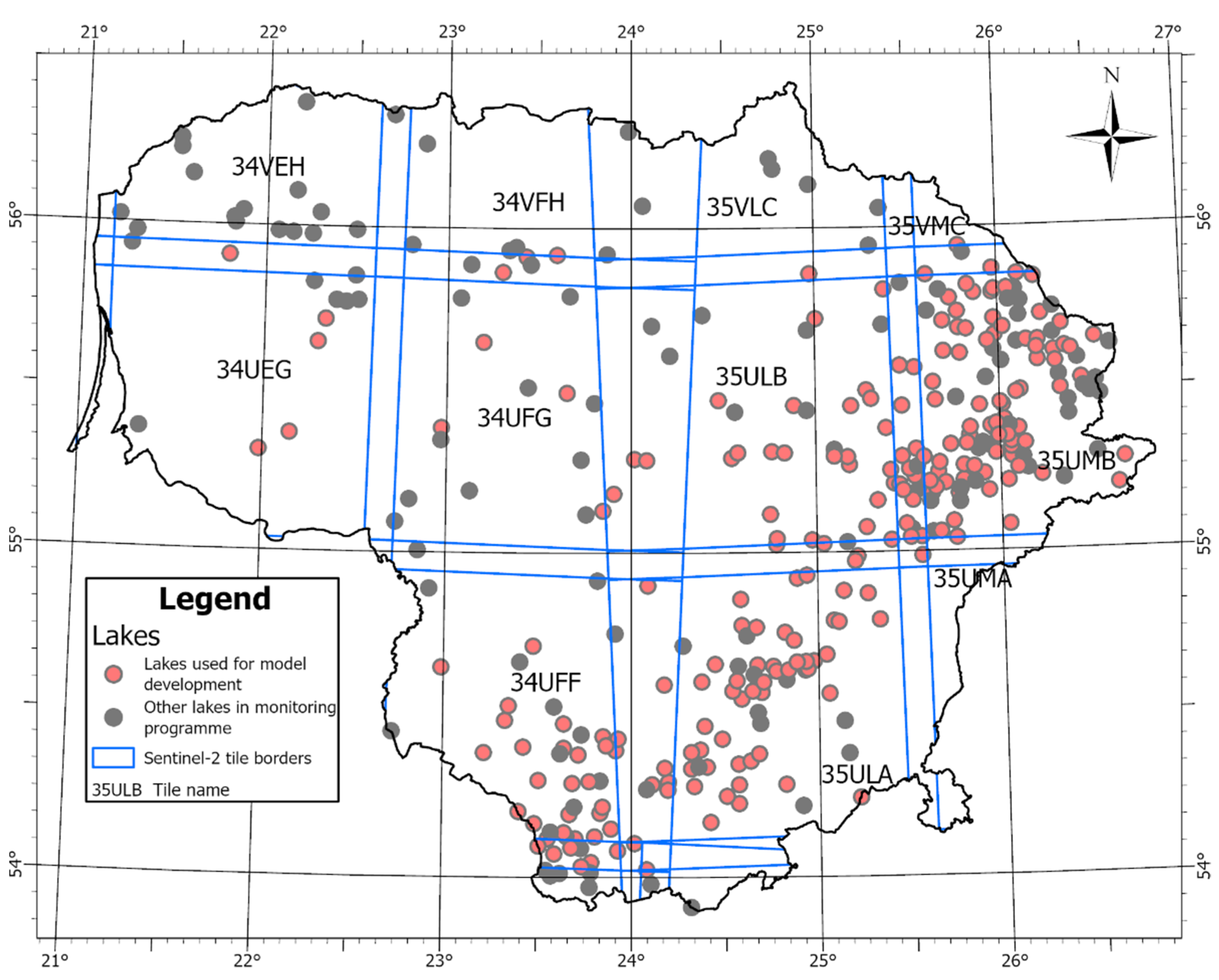
There are 357 lakes and ponds included in the national monitoring programme in Lithuania. They are covered by 11 Sentinel-2 tiles (Figure 1). Most of the lakes are larger than 0.5 km2.
2.2. In Situ Dataset and Grouping Measurements
An in situ dataset was obtained from the Lithuanian Environmental Protection Agency under the Ministry of Environment. The data are collected under the state monitoring programme of lakes and ponds. We used chlorophyll-a concentration (chla), water transparency (Secchi disk depth), and suspended matter (SM) concentration data from the years 2015–2020.
We used in situ data to assign each measurement a biophysical class—a target label for further use in creation of classification algorithm. Water transparency characterises the ecological status in general and is directly related to optically active substances such as chlorophyll concentration, SM concentration and the amount of coloured dissolved organic matter. We used lake types defined based on their depth [24], and lake ecological status class definition based on water transparency. Ecological status of a shallow lake (type 1, average depth < 3 m or average depth > 3 m and maximum depth < 11 m) is considered good or high when water transparency is higher than 1.3 m while for medium deep (type 2, average depth > 3 m and maximum depth 11–30 m) and deep lakes (type 3, maximum depth > 30 m) the status is considered good or high when transparency is > 2 m. Lower than 1.3 m water transparency for a shallow lake and lower than 2 m transparency for medium deep and deep lakes is considered of moderate, poor, or bad ecological status [25]. In addition, as chla is a good proxy for the trophic state of a lake, we selected two chla thresholds to group chla measurements into three groups. We used a threshold for chla concentration based on the definition of the Carlson’s trophic state index [26], where oligotrophic and mesotrophic lakes (low bioproductivity waters) have concentrations lower than 7.2 mg/m3, eutrophy (fairly high bioproductivity waters) is defined with concentrations 7.2–20 mg/m3, and hypereutrophy (high bioproductivity waters) with concentrations higher that 20 mg/m3 (Table 1). We used measurements of another optically active substance—SM and divided measurements into two groups—lower than 10 mg/m3 and higher than 10 mg/m3. By combining classes based on different parameters we formed 12 classes (Table 1). A class 1_clear is characterised by low concentrations of parameters as well as good transparency, this is also the class containing the most measurements (46% of total). The next large class 2_chla_clear is characterised by higher chla concentration; but good transparency and low SM amount. Thus, in this class the main optically active substance found was chlorophyll. It contained 21% of all measurements. Another larger class was 3_chla_turbid; however, it contained only 9% of data, this class was also dominated by chlorophyll and turbidity that caused it to have moderate, bad or poor ecological class based on water transparency. Other classes had 0 to 7% of cases. There were very few cases where SM was dominant (1_SM_turbid, 2_chla_SM_turbid classes), thus it was not included in the training-test set for machine learning algorithms.
At first, we wanted to see if machine learning models can separate the lakes where transparency is good, and optically active substances are found in low concentrations. We defined this class as Clear (based on 1_clear class, Table 1). Separating the Clear class from the others provides an opportunity to distinguish measurements that are not of a particular concern as there are very low amounts of dominating optically active substances in them, therefore, not posing any problems. Therefore, we used Clear and OAS-class (for lakes with significant amounts of optically active substances), as target labels for a binary classification task. We omitted classes that had 0–2 cases as they are not common and would likely be misclassified by machine learning algorithms that generally require a large number of samples. The binary classification task is slightly imbalanced with 46% of cases in the Clear class and 54% in the OAS-class.
The next step was to distinguish different water bodies in the OAS-class to water bodies (Table 1) that are characterised by:
- Good or high transparency class, despite the presence of some optically active substances. Chla is the dominating substance in this class. The label for the class is Moderate.
- Most water bodies have high turbidity due to high chla concentration, in some cases due to both high chla and SM concentration. The class label is Chla-dominated.
- Higher turbidity due to reasons other than phytoplankton and SM concentration. These lakes are likely to have higher coloured dissolved organic matter (CDOM) content.
In multi-class classification step, classes were more imbalanced—the 39% of cases were of the Moderate class, 43% in the Chla-dominated class, and 18% of cases were in the Turbid class.
2.3. Sentinel-2 Dataset
We used optical Sentinel-2 MSI data. A total of six Sentinel-2 tiles that cover a large area of Lithuania were used in this study: T34UEG, T34UFG, T35ULB, T35UMB, T34UFF, T35ULA (Figure 1). We downloaded tiles that had lower than 30% cloud cover from the Copernicus Open Access Hub of the European Space Agency.
We used the Sen2Cor atmospheric correction algorithm with 20 m resolution. The data were then filtered, removing no data pixels, then using scene classification—only water pixels (flag—6) were kept. In addition, we applied further filtering based on the shortwave infrared band B11 (1610 nm). We retained spectra with lower reflectance than 0.0215 in band B11. This filtering threshold is commonly used for the separation of water from non-water pixels as it is assumed that at these wavelengths water-leaving radiance is zero [27].
We extracted a 3 × 3 pixel area centred at the national monitoring site location in the lake. To remove any suspicious pixels likely affected by clouds, we performed filtering based on the 783 nm band (B7). Pixels where the standard deviation of the 3 × 3 pixel was lower than 0.002 were retained.
For further analysis we used observations that were within a plus or minus three day time period: situ date plus or minus three days of satellite acquisition. For example, if we have an in situ measurement on the 15 June, a closest cloudless satellite observation was used from the 12 to 18 June. This time window was chosen due to the small number of concomitant measurements of in situ and satellite, and as for training we needed to have the largest dataset possible. We assumed that there would not be large changes within objects and that satellite spectra would still be representative. The final dataset that we used for training had 563 measurements—in situ data with accompanying satellite spectra. This included 226 different lakes and ponds.
2.4. Machine Learning Algorithms
We used six supervised machine learning algorithms that can be used for binary and multi-class classification problems:
Logistic regression (LR) is a parametric linear model, used to model a probability of a discrete number of outcomes. In the beginning we calculate the weighted sum of inputs (features) and then feed it to the sigmoid function and the probability is returned. Then it is converted to a binary output, 0 or 1.
Support vector machine (SVM) aims to find a hyperplane that best divides the data. The decision function depends on a subset of data (support vectors) that are closer to the hyperplane separating two classes. The data can be transformed using a linear, radial basis, polynomial, sigmoid or other function. SVM is often more accurate for small datasets and when there are many features [28].
Random forest classifier (RF) is an ensemble model that uses many decision trees to decide to which class a sample belongs. Individual decision trees divide data by a series of decision rules based on feature data and selected thresholds of them. For a sample the class is assigned that most decision trees voted for. Random forest uses bootstrap aggregation allowing decision trees to sample data and in this way creating different trees. In addition, in random forest, trees are allowed to subset not all features but only a random subset of them that decreases the correlation between the trees [29].
AdaBoost classifier (Ada) is an adaptive boosting technique from the ensemble models family. The name “adaptive” is explained as the weights being re-assigned to each sample, with higher weights to incorrectly classified samples [30]. Any machine learning algorithm can be used inside AdaBoost; however, we used the default version that used decision trees.
XGBoost Classifier (XGB). XGBoost stands for eXtreme Gradient Boosting. It is a decision-tree based ensemble model that uses a gradient boosting technique [31]. XGB algorithm progressively adds more and more branches (if conditions) to the decision tree to build a stronger model. Generally, it is a fast and well performing algorithm.
Artificial Neural Networks (ANN) is a complex algorithm that is harder to interpret than other machine learning algorithms as it often includes at least several hidden layers [32]. In addition, it requires optimisation of many hyper-parameters. However, ANNs in many cases provide the most accurate results, thus ANNs are widely implemented in many fields including remote sensing data analysis [33,34,35].
2.5. Workflow
All the data preparation was implemented in the Rstudio environment [36], while machine learning algorithms were trained in the python environment using scikit-learn module [37] for LR, SVM, Ada, and RF, XGBoost module [31] for XGBoost classifier, and keras for ANN [38]. We used class weights to compensate for class imbalance (Table 2).
Training-testing workflow:
- 1.
- Calculate features. For model training we used features derived from lake spectrum: reflectance amplitude—the maximum reflectance at the 490–865 nm wavelengths minus the minimum reflectance at the 490–865 nm wavelengths, band ratios R705/R665, R560/R490, R560/R665, and R560/R705, band differences BD1 and BD2, an empirical equation that uses BD2, apparent visible wavelength (AVW), hue angle, colour based on Forel-Ule colour scale (FU), and a month that could help to separate blooming conditions as they more frequently occur in summer time (Table 3).
- 2.
- Split data into train set (80%) and test set (20%) based on lakes (all observations of one lake go to either train or test set so that the model would not learn a particular combination of parameters characteristic to a specific lake). Test set is held out until the model evaluation step. There were 440 data points (observations) in the training set and 123 data points in the test set (563 in total) for the binary problem. For the three-class problem we had 245 data points in the train set and 58 data points in the test set (303 in total).
- 3.
- Transform features to a Gaussian distribution using the PowerTransform() function from scikit-learn.
- 4.
- Scale feature data based on the training dataset (mean and standard deviation) using the function StandardScaler() from scikit-learn. Data scaling is recommended when using any machine learning algorithm.
- 5.
- Train models using the same split of data without setting any hyper-parameters.
- 6.
- Evaluate models using stratified three-fold cross-validation and on test set using evaluation metrics (accuracy, precision, recall, F1, area under curve (AUC) score, and log_loss) found in the scikit learn module. The Stratifiedkfold technique performs the training set data split to folds based on groups of target labels. In the three-fold case, the training dataset is split three times into three equal size parts [A, B, C]. The first time parts A and B are used as a training dataset, while part C is used as a validation set based on which model performance metrics are calculated. The second time and third time other parts are used as validation sets.
- 7.
- Select the best performing algorithm and optimise its hyper-parameters using training dataset and stratified three-fold cross-validation. Hyper-parameter search was performed using the optuna module for python. Optuna is a fast automated hyper-parameter search optimization technique [45].
- 8.
- Apply the created model on 226 lakes that were at least once found in the matchup dataset, and analyse the results.
2.6. Model Performance Metrics
To evaluate model performance and compare them with each other we used several metrics:
Confusion matrix—a classification table where a number of correct and incorrect predictions are calculated across a class (Table 4).
In this study, true positives are correctly classified Clear class observations, false positives—correctly classified OAS-class observations, while false positives mean the incorrectly classified cases from Clear class, and false negatives—falsely classified observations from the OAS-class observations.
Accuracy Equation (1)—a fraction of correct predictions of all classes.
Precision Equation (2)—the ratio between the number of true positives and the number of positively predicted samples. The precision defines the ability of a classifier not to label negative samples as positive. For example, in our case, it shows what part of all the predictions labelled as Clear class were correctly predicted.
Recall Equation. (3)—the ratio of true negatives and negatively predicted samples. In our case recall shows the ability of a classifier to classify OAS-class examples. The best score is 1, and the worst is 0.
F1 score Equation (4)—is a weighted average of precision and recall. The relative contribution of precision and recall is equal. In the multi-class case, this is the average of F1 score for each class with weighting depending on the average parameter.
AUC—area under the Receiver Operating Characteristic Curve (ROC AUC) calculated from prediction scores. ROC curve plots two parameters—true positive rate (TP/(TP + FN)) and false positive rate (FP/(FP + TN)). The AUC measure is an integral underneath the entire ROC curve. A value of 0.0 describes a model without any predictive skill, 0.5—a model that predicts as well as a random guess (in binary classification), and a value of 1.0 shows that model predictions are 100% correct. An AUC of 0.7 shows that there is a 70% chance that model will distinguish between two classes.
Log_loss or cross-entropy loss is the loss function defined as the negative log-likelihood of a model that returns probabilities of predictions for its training data. A lower log_loss means better predictions.
3. Results
3.1. Classification Using In Situ Measurements
We grouped measurements in lakes to four classes based on concentrations of chla and SM, transparency, and depth. The chla and SM are the optically active substances in water, while transparency characterises the overall ecological status of a water body. Depth information also contributes to the definition of ecological state of a water body and may help to separate naturally old and eutrophic lakes. The Clear class had a mean chla concentration of 3.8 mg/m3 and mean transparency of 4.5 m (Table 5), while the Moderate class had a higher chla concentration (mean 11.7 mg/m3) and lower than the Clear class transparency (mean 2.5 m). The other two classes had mostly moderate, bad, or poor ecological status. The Chla-dominated class was characterised by algal blooms while water bodies in the Turbid class had low transparency despite not very high chla concentrations as in the Chla-dominated class. These classes were used as target labels in machine learning algorithms.
3.2. Significant Features for Building Models
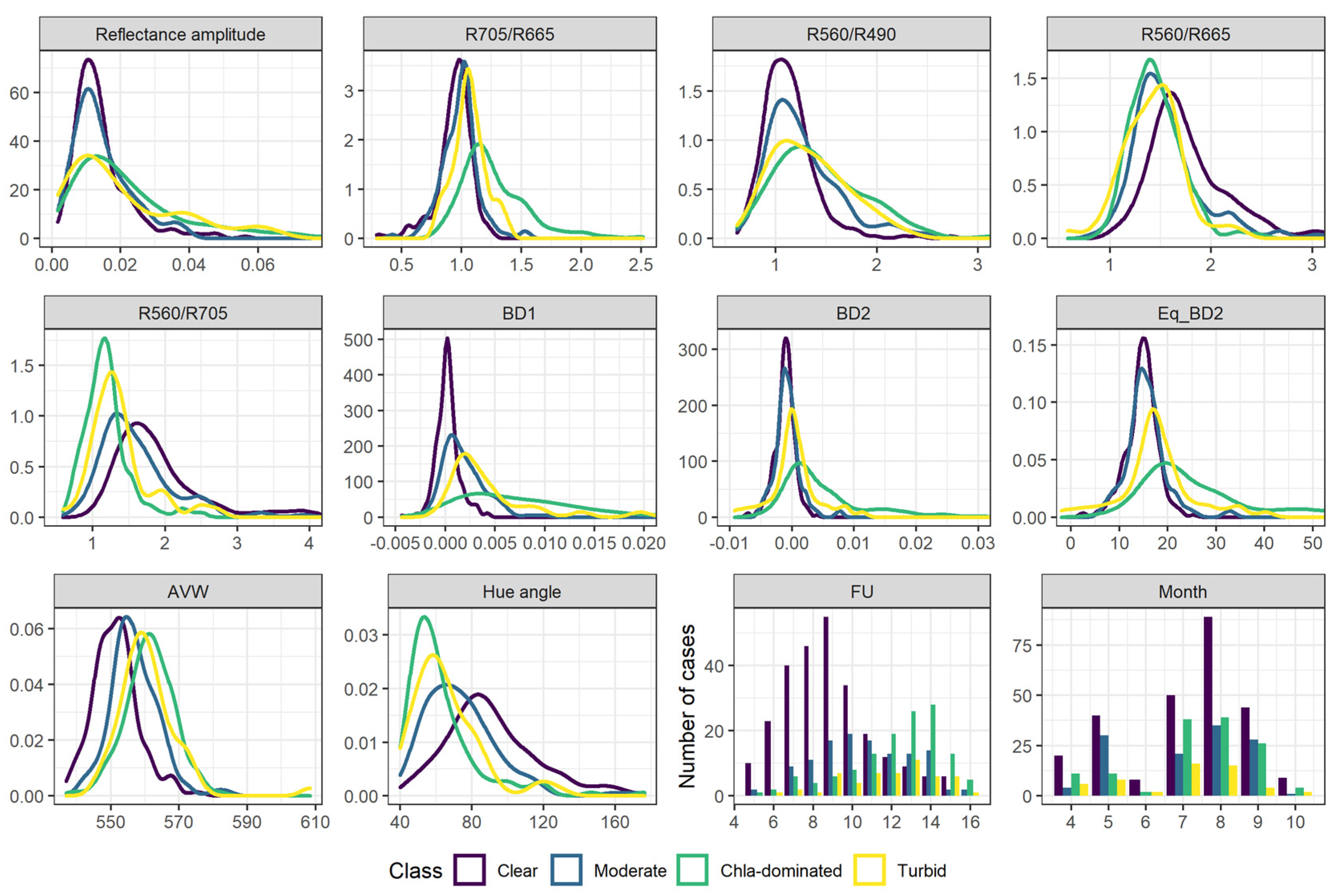
Absence of multicollinearity is an important assumption for regression models to provide meaningful and interpretable results. Other types of algorithms also tend to work better when there is a low correlation between the features. We calculated the correlation between the features and between the features and labels (Table 6). The features that we inspected can be grouped into two groups: those that are directly derived from reflectance —either the band difference or band ratio, and another group—more complicated features derived from several bands (AVW, hue angle, and FU). Since AVW, hue angle and FU are highly correlated among each other (r = −0.94, 0.9, and 0.94) we decided to use one of them —AVW, as it showed the highest correlation with the target label. In addition, features’ distribution showed better separability of classes using AVW as the dominant colour describing wavelength moves towards the longer wavelengths, from the Clear to the Chla-dominated class (Figure 2). From the other group of features, we selected BD1 and R560/R705 as they are less correlated to each other than other features (r = −0.23) and have relatively high correlation with the target label (r = −0.38 and r = 0.3, respectively). We selected three features, also based on preliminary results obtained with logistic regression as the multicollinearity impairs the performance of this algorithm. It is possible to obtain an explanation with these features. An increase in R560/R705 feature value by one unit increases the odds of a lake to be classified as Clear by 1.7, while increasing BD1 and AVW values by one unit would decrease the odds of a lake to be assigned to the class Clear (Table 7).
3.3. Model Validation and Testing Results
3.3.1. Binary Problem
In the first step, we aimed to separate lakes that have low quantities of optically active substances (chla and SM) and therefore are characterized by high water transparency (Clear class).
The models showed 79–81% accuracy on the validation set (Table 8). We used three-fold cross-validation to reduce the impact of individual model runs and to have better generalization opportunities. Cross-validation results showed that there is some variance in model performance; however, the standard deviation of accuracy between different folds was up to 0.03 for SVM and ANN models and 0.02 for AUC score for AdaBoost.
Model performance was generally quite similar among the models; however, based on the AUC score, the best performance on unseen data was observed for RF (Table 9). In addition, the RF provided the lowest log_loss value, showing good performance of the model. In our model, the label 1 was assigned to the Clear class, therefore, not only the true positives are important, but also that a lake with some optically active substances would not get the Clear lake class. Thus, a low number of false negatives is preferred. We decided to use the RF model as it provided the lowest number of incorrectly classified lakes (n = 19 from the total of 123), as well as a relatively low number of false negatives (n = 7). Moreover, RF is not sensitive to feature multicollinearity, thus, it is a better choice than LR, that showed similar performance on this dataset; however, predictions with it could be affected by multicollinearity. We tried to optimise the hyper-parameters for the RF model; however, that did not improve model accuracy, thus, we decided to use the first version of it. The most important feature in the RF classifier was BD1 (relative importance = 0.4), while R560/R705 and AVW shared the same importance (0.30) for trees construction in the RF.
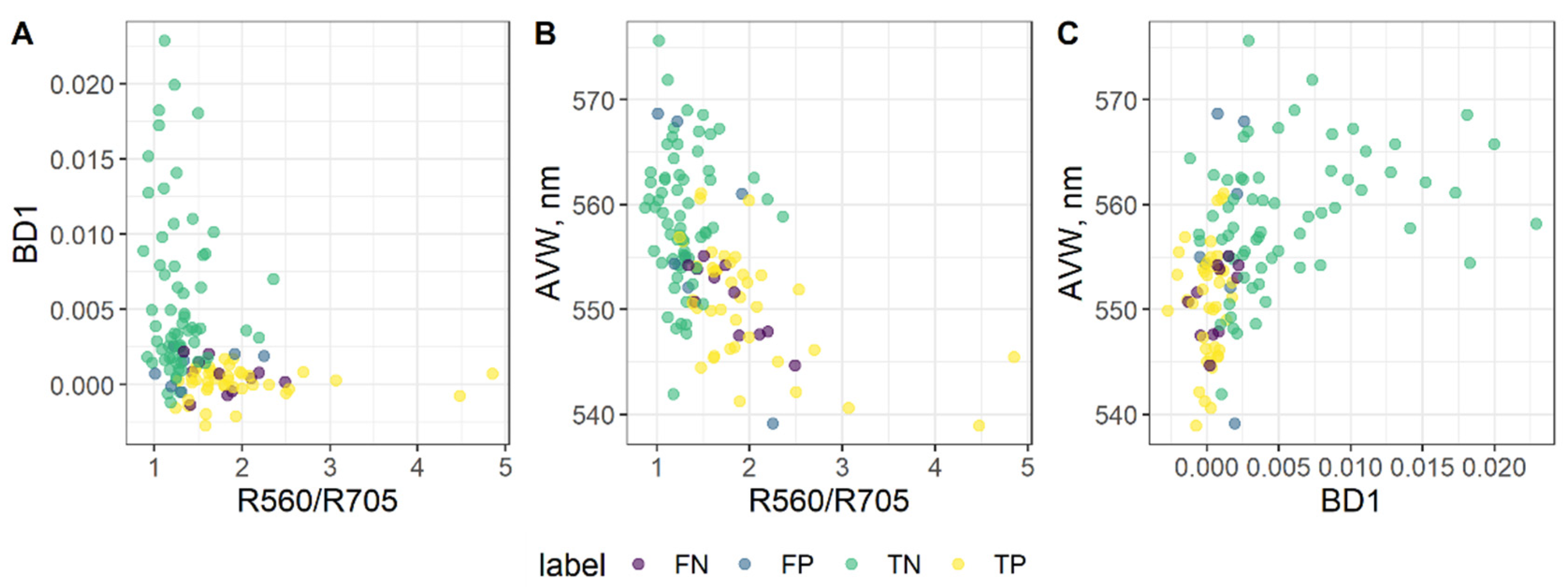
The test set that we used had 123 data points, from which 19 data points were misclassified by the RF classifier. Most of the misclassified points were from the OAS-class (12) and were given a class label of Clear (false positives) (Table 9). The values distribution of the most important feature, BD1, of the true positives (correctly classified Clear class observations) show that values centre close to zero (median = 0.0003) (Figure 3), while most of the true negatives have higher values (median = 0.004). The values of BD1 of FN (median = 0.0008) are similar to the TP values and the values of FP (median = 0.002) are closer to the TN values. A similar situation is observed with the other features also (Figure 3). The median chla concentration was 10.3 mg m−3 of these incorrectly classified data points showing that most of the data points with high chla concentrations were assigned a correct class.
3.3.2. Multi-Class Problem
Further, we explored the OAS-class that was composed of measurements from lakes that have substantial amounts of optically active substances—chla and SM. We classified lakes into three groups: Moderate (having some chla; however, good and high transparency), Chla-dominated (turbid due to chla and/or SM and characterized by low transparency), and Turbid (turbid due to other reasons, likely due to higher amounts of coloured dissolved organic substances). Such biophysical classification allows the ability to distinguish light and strong algal blooms, and turbid waters.
Since the best performance in the two-class problem was observed for RF, we decided to use RF for the three-class problem too. RF is not sensitive to feature multicollinearity and since our dataset is small, we tried using RF with all the 12 features. However, this did not provide us with the results expected, thus, we used features that had some differences in their distribution by class (Figure 2), especially noticing the differences between features’ distribution of Moderate and Chla-dominated classes, as the Turbid class was not that abundant in our dataset. We used three features—reflectance amplitude, R705/R665 ratio, and AVW. The relative importance was the highest of R705/R665 feature—0.38, while relative importance for each other feature was 0.31. The accuracy on unseen data among the classes varied from 27% to 81% (Table 10). Hyper-parameter optimization did not change the overall accuracy; however, it improved the classification of the Turbid class, nonetheless the number of false positive for other classes increased as well. We decided to use the version of RF model without hyper-parameter optimization to keep the higher accuracy of the larger classes—Moderate and Chla-dominated.
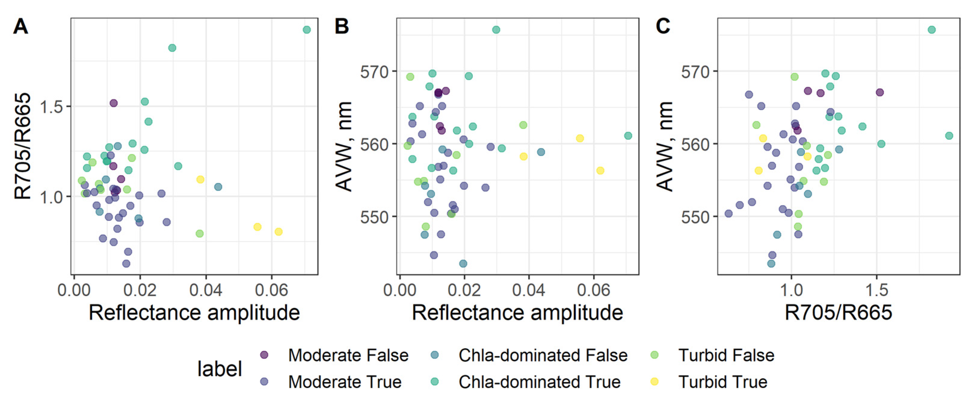
The features’ values of incorrectly classified observations in some cases overlap with the values of other classes (Figure 4). The values of features of incorrectly classified observations from the Chla-dominated class are similar to the values of correctly classified observations from the Moderate class. This is observed as the class boundary is strict while similar feature values might be related to different classes.
3.4. Biophysical Lake Classification Using Random Forest Model
We applied a two class model on 19,292 lake spectra from 226 lakes from a six-year period 2015–2020. There were from 17 to 112 observations for a lake (mean = 85, standard deviation, sd = 15). The 59.7% of lake spectra were classified as Clear, thus the three-class model was applied to the rest of the spectra (7764) and 22.7% were classified as Moderate, 17.0% got the Chla-dominated class, and 0.6% the Turbid class.
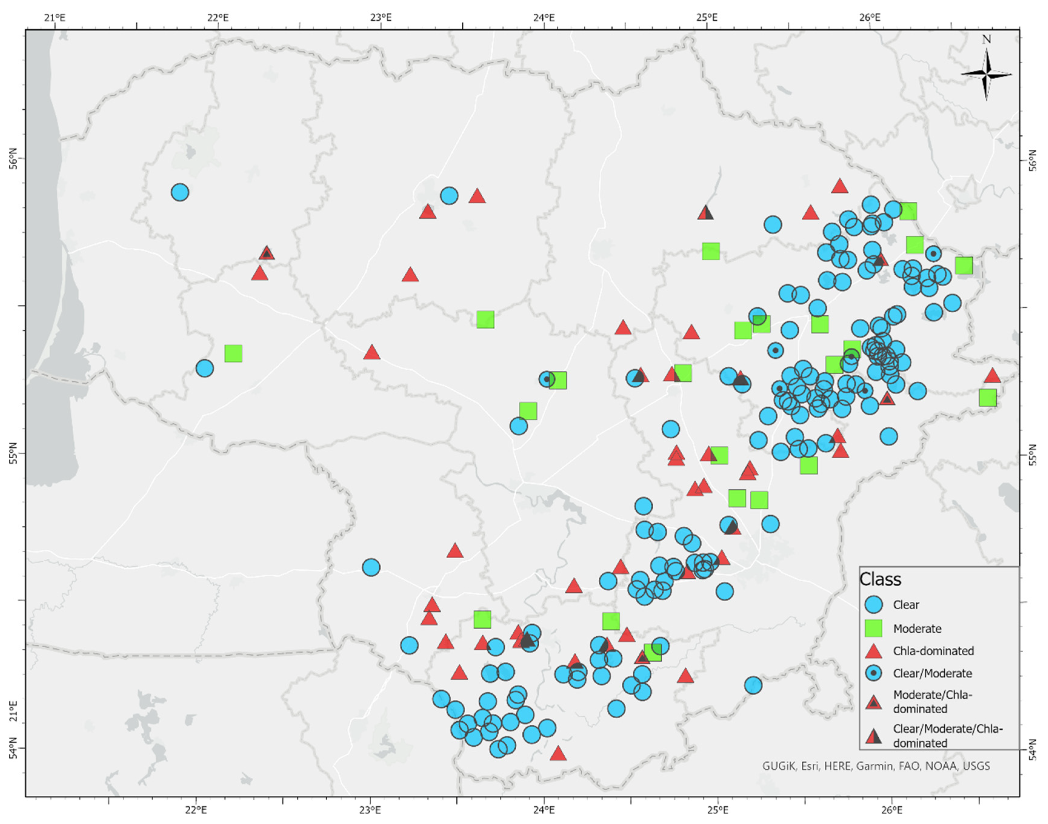
The Clear class was the most prevalent as it was attributed as the most frequent class throughout 2015–2020-year period to 151 lakes, from which in 110 lakes this class was the most frequent class in all the years in this time period (Figure 5). There were changes of class in these lakes throughout the April-October season and other classes were also observed in some of these lakes. The Moderate class was observed in almost all of these lakes (108); however, the average percentage of observations attributed to this class was 18% (sd = 11%). Some occurrences of the Chla-dominated class were observed in 88 of these lakes; however, only 9% (sd = 5%) of observations were characterised by this class. The Turbid class was observed on average in 6% (sd = 2%) of observations in 22 of these lakes. The highest average percentage (97%, sd = 8%) of observations of the Clear class were in the year of 2015, while the lowest (78%, sd = 14%) were in the year of 2018. The Chla-dominated class was observed at least once in 49 lakes in the year of 2020 and thus this class constituted 11% (sd = 5%) of observations on average. In 11 lakes there were two consecutive observations in time of the Chla-dominant class, mostly in the months of April and September, thus these lakes require further analysis.
In 41 lakes we observed class instability throughout years; however, the Clear class was the most frequent and mostly class change was observed between the Clear and Moderate classes. Nonetheless, there were 11 lakes in which in one of the years the Chla-dominated was the prevalent class; however, in some cases it was in the year of 2015, and that year there were a lower number of observations, and they started in summertime due to the launch of the satellite at the end of June. In total, in 26 lakes from this group of lakes, the Chla-dominated was observed in different seasons in different years.
In the Moderate class the change of class occurred more often and there were just seven lakes where Moderate was the prevalent class (the mean percentage of this class from total number of observations was 68%, sd = 13%) throughout six years. In these lakes Clear was the second most occurring class (mean = 23%, sd = 12%). In six lakes out of seven lakes Chla-dominated occurred on average 20% of observations (sd = 10%), and Turbid in four lakes—mean = 7%, sd = 3%. In others where Moderate was the prevalent class but with class change throughout years, there was a larger change towards the Chla-dominated class.
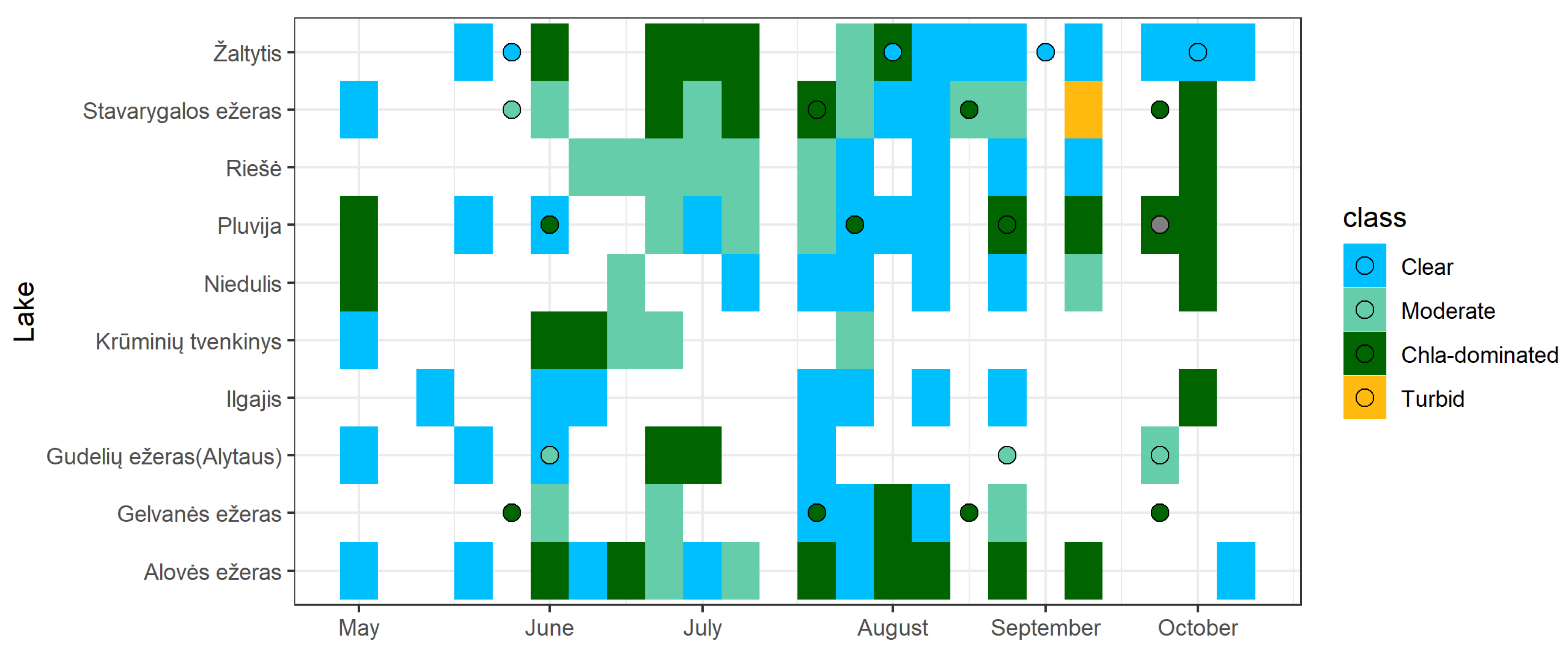
The Chla-dominated class is likely related to algal blooms. This class was prevalent in 42 lakes and in 20 of those lakes the prevalent class obtained from satellite data and RF models was the same for the six-year period. In these lakes every year this class was attributed from 40 to 100% of observations showing the different length of algal blooms in these lakes. In several lakes there was very little of change of class (Lake Ūdrijos, Lake Didžiulis (Dusmena), and Petraičių pond)—in all years in the spring to autumn season these lakes were characterised by algal blooms (89–100% of observations assigned to the Chla-dominated class). More class changes were observed in other Chla-dominated lakes. In others, yearly class change was observed and in 45% of these lakes other classes than Chla-dominated were observed in the year of 2020. There were from 6 to 19 observations in these lakes in the year 2020 (Figure 6). In some lakes in spring and autumn there was the Chla-dominated class, while in summertime we observed the Clear and Moderate classes (Lake Niedulis), that in some cases did not reflect in situ measurements (Lake Pluvija). The RF models likely misclassified lake classes in summertime in these lakes.
There were no lakes where the Turbid class was identified as the most frequent in at least one year, based on satellite data. There were also 11 lakes where we could not discriminate the prevalent class as there were equal number of years with two or three classes. In some cases, yearly class selection was influenced by a small number of observations in different seasons, thus it might have happened that the prevalent class was determined from spring and autumn observations while lacking summer observations when algal blooms are expected in some lakes. In addition, there were cases when the model misclassified the class when in situ data were available.
4. Discussion
We created a model based on a random forest machine learning algorithm that, using spectral features, can classify lake observations into four classes—Clear, Moderate, Chla-dominated, and Turbid classes. Firstly, the model separates observations with Clear class from others (those having some optically active constituents) and then the second model classifies the other observations (OAS-class) into three classes: Moderate, Chla-dominated, and Turbid. Having two steps of classification helps to separate the observations that are characterised by clear conditions with low amounts of optically active constituents. Those are nonproblematic cases.
The classes were defined by routinely observed water quality parameters, such as, chla concentration, water transparency, and suspended matter concentration that determines the ecological state of a water body. The Moderate and Turbid classes were similar based on chla, and similar to the Clear class based on SM (Table 5). However, the Turbid class was more similar to the Chla-dominated class based on transparency values. Some similarities may have caused misclassification of observations as the formation of classes was based on strict threshold values of water quality parameters. Spectral similarity of the Turbid class to the Clear and Moderate classes as seen from computed spectral features (Figure 2, Figure 3 and Figure 4) contributed to the low classification accuracy on unseen data that was 27% for the Turbid class while for the Clear class the accuracy was much higher—85%. In addition, there was a lower number of observations in the Turbid class (53 in total), while there were 260 observations of the Clear class. We chose more distinct features (Figure 2) and used class weights (Table 2) to improve classification accuracy; however, it is likely that increasing the number of observations could improve the classification accuracy further.
The classification accuracy of cases of the Chla-dominated class defining low transparency algal blooms was lower than the classification accuracy (72%) for cases in the Clear class. However, after performing a visual inspection of RGB images it turned out that 43% of misclassified cases were related to thin clouds or cloud shadows’ influence on satellite data. Sen2Cor image classification that we used for filtering non-water pixels failed to mask out the thin clouds and cloud shadows in these cases; though the problem is known, fixing it over water bodies with low signal remains challenging and the use of several scene classification algorithms can be an option to increase scene classification accuracy [46]. In those cases (for example, Lake Pluvija in 2020, (Figure 6) spectral signal was reduced and chla signal was not registered by satellite. In this study we used Sentinel-2 MSI tiles with up to 30% of cloudiness, though using images with higher cloudiness could expand the training-test set; however, another or additional data quality check is necessary to ensure data quality. In other cases, mostly (43% of cases) there was two-three days’ time difference between the in situ measurement and the satellite observation, thus, conditions in a lake could have changed and the observation was assigned to the Moderate class. Nevertheless, a model can be used for identification of the prevalent class in a lake (Figure 5) and class change throughout the season identifying light (Moderate class) and strong algal blooms (Chla-dominated). It can help for determination of algal bloom onset and dynamics when class change is observed, thus, it can serve as an additional tool to in situ measurements.
There are a lot of machine learning algorithms that can be used to solve the same problem; however, it is advisable to use the simplest method possible yielding the best results. In our study we built models based on a random forest algorithm that is often used for its interpretability and ability to extract important features. The random forest provided the best results in our study as well as in other studies in chlorophyll retrieval [47,48] and more complex algorithms such as ANN provide just slightly better results [49].
Our classification model can be applied to other regions where similar classes are observed without retraining. Our model was created based on observations from 226 lakes and is focused mostly on waters dominated by phytoplankton. We also included turbid due to other reasons waters into the Turbid class; however a better description of this class, for example, with absorption coefficients at 440 nm, that is a good descriptor of coloured dissolved organic matter content [50], is needed to improve model results. In other regions, the class definition described in Table 1 could be extended with this parameter and different class aggregations could be used. Our model could be extended with more classes, such as, a class dominated by SM (for example, 1_SM_turbid class as in Table 1). In that case a model should be retrained, and inclusion of new spectral features should be reviewed.
Biophysical classification of lakes can be a tool for experts at regional environmental protection agencies. It can help to observe sudden changes in a lake remotely and make decisions on carrying out the measurements in situ. The classification can serve as a tool to observe onset and dynamics of algal blooms. In this way it can inform on the state of a lake in between the in situ measurements. Additionally, biophysical classes can be used to develop water parameter retrieval algorithms from satellite data.
5. Conclusions
The machine learning algorithms were tested to create a model for biophysical classification of lake observations using Sentinel-2 MSI data as input. The most accurate model for separating Clear and OAS-class observations was obtained using random forest classifier with BD1, R560/R705, and AVW features as input. This step allowed us to separate observations that are characterised by low amounts of optically active substances (chla and SM) from those with significant amounts of these substances (OAS-class). The random forest classifier with reflectance amplitude, R705/R665, and AVW as input was then used to determine the Moderate, Chla-dominated, Turbid lake observations. The classification accuracy when models were applied on unseen data, varied from 27% for the Turbid class, to 85% for the Clear class, while accuracy of classification of classes related to algal blooms were 81% (Moderate) and 71% (Chla-dominated). The classification accuracy for classes could be increased by enlarging the training-test dataset and ensuring better removal of observations that were affected by cloud shadows and thin clouds.
The models were applied to 19,292 lake spectra of 226 lakes in Lithuania that are larger than 0.5 km2 and are monitored according to a state monitoring programme. The prevalent class over the 2015–2020-year period was Clear (151 lakes); however, 42 lakes were affected by likely strong algal blooms. In addition, we were able to use biophysical classes to observe changes in lakes through the years 2015–2020, and throughout the warm (April-October) season. Our biophysical lake classification models can be applied to other regions where phytoplankton is the dominant substance found in water. Additionally, models can be expanded by including new classes (for example, SM-dominated). Biophysical classification of lake observations can be helpful to experts in the regional environmental protection agencies and also introduced to the public as a simple characterisation of a water body.
Author Contributions
Conceptualization, D.G. and E.S.; methodology, D.G.; software, D.G.; validation, D.G.; formal analysis, D.G.; data curation, D.G.; writing—original draft preparation, D.G.; writing—review and editing, E.S. and D.G.; visualization, D.G.; supervision, E.S.; project administration, D.G.; funding acquisition, D.G. All authors have read and agreed to the published version of the manuscript.
Funding
This research was funded by Vilnius University Research Promotion Fund grant No. MSF-JM-7/2021.
Data Availability Statement
Not applicable.
Conflicts of Interest
The authors declare no conflict of interest. The funders had no role in the design of the study; in the collection, analyses, or interpretation of data; in the writing of the manuscript, or in the decision to publish the results.
References
- Tranvik, L.J.; Downing, J.A.; Cotner, J.B.; Loiselle, S.A.; Striegl, R.G.; Ballatore, T.J.; Dillon, P.; Finlay, K.; Fortino, K.; Knoll, L.B.; et al. Lakes and reservoirs as regulators of carbon cycling and climate. Limnol. Oceanogr. 2009, 54, 2298–2314. [Google Scholar] [CrossRef] [Green Version]
- Schindler, D.E.; Scheuerell, M.D. Habitat coupling in lake ecosystems. Oikos 2002, 98, 177–189. [Google Scholar] [CrossRef] [Green Version]
- Woolway, R.I.; Dokulil, M.T.; Marszelewski, W.; Schmid, M.; Bouffard, D.; Merchant, C.J. Warming of Central European lakes and their response to the 1980s climate regime shift. Clim. Chang. 2017, 142, 505–520. [Google Scholar] [CrossRef]
- Yao, F.; Wang, J.; Wang, C.; Crétaux, J.-F. Constructing long-term high-frequency time series of global lake and reservoir areas using Landsat imagery. Remote Sens. Environ. 2019, 232, 111210. [Google Scholar] [CrossRef]
- Modabberi, A.; Noori, R.; Madani, K.; Ehsani, A.H.; Mehr, A.D.; Hooshyaripor, F.; Kløve, B. Caspian Sea is eutrophying: The alarming message of satellite data. Environ. Res. Lett. 2020, 15, 124047. [Google Scholar] [CrossRef]
- Sun, D.; Li, Y.; Wang, Q. A Unified Model for Remotely Estimating Chlorophyll a in Lake Taihu, China, Based on SVM andIn SituHyperspectral Data. IEEE Trans. Geosci. Remote Sens. 2009, 47, 2957–2965. [Google Scholar] [CrossRef]
- Al-Kharusi, E.S.; Tenenbaum, D.E.; Abdi, A.M.; Kutser, T.; Karlsson, J.; Bergström, A.-K.; Berggren, M. Large-Scale Retrieval of Coloured Dissolved Organic Matter in Northern Lakes Using Sentinel-2 Data. Remote Sens. 2020, 12, 157. [Google Scholar] [CrossRef] [Green Version]
- Kutser, T.; Paavel, B.; Verpoorter, C.; Ligi, M.; Soomets, T.; Toming, K.; Casal, G. Remote Sensing of Black Lakes and Using 810 nm Reflectance Peak for Retrieving Water Quality Parameters of Optically Complex Waters. Remote Sens. 2016, 8, 497. [Google Scholar] [CrossRef]
- Soomets, T.; Uudeberg, K.; Jakovels, D.; Brauns, A.; Zagars, M.; Kutser, T. Validation and Comparison of Water Quality Products in Baltic Lakes Using Sentinel-2 MSI and Sentinel-3 OLCI Data. Sensors 2020, 20, 742. [Google Scholar] [CrossRef] [Green Version]
- Grendaitė, D.; Stonevičius, E. Uncertainty of atmospheric correction algorithms for chlorophyll α concentration retrieval in lakes from Sentinel-2 data. Geocarto Int. 2021, 1–25. [Google Scholar] [CrossRef]
- Maier, P.M.; Keller, S. Estimating chlorophyll a concentrations of several inland waters with hyperspectral data and machine learning models. arXiv 2018, arXiv:1904.02052v1. [Google Scholar] [CrossRef] [Green Version]
- ESA Gearing up for Third Sentinel-2 Satellite. Available online: https://www.esa.int/Applications/Observing_the_Earth/Copernicus/Sentinel-2/Gearing_up_for_third_Sentinel-2_satellite (accessed on 21 April 2022).
- Spyrakos, E.; O’Donnell, R.; Hunter, P.D.; Miller, C.; Scott, M.; Simis, S.G.H.; Neil, C.; Barbosa, C.C.F.; Binding, C.E.; Bradt, S.; et al. Optical types of inland and coastal waters. Limnol. Oceanogr. 2018, 63, 846–870. [Google Scholar] [CrossRef] [Green Version]
- Reinart, A.; Herlevi, A.; Arst, H.; Sipelgas, L. Preliminary optical classification of lakes and coastal waters in Estonia and south Finland. J. Sea Res. 2003, 49, 357–366. [Google Scholar] [CrossRef]
- Uudeberg, K.; Ansko, I.; Põru, G.; Ansper, A.; Reinart, A. Using Optical Water Types to Monitor Changes in Optically Complex Inland and Coastal Waters. Remote Sens. 2019, 11, 2297. [Google Scholar] [CrossRef] [Green Version]
- Da Silva, E.F.F.; de Moraes Novo, E.M.L.; de Lucia Lobo, F.; Barbosa, C.C.F.; Noernberg, M.A.; da Silva Rotta, L.H.; Cairo, C.T.; Maciel, D.; Júnior, R.F. Optical water types found in Brazilian waters. Limnology 2020, 22, 57–68. [Google Scholar] [CrossRef]
- Ioannou, I.; Gilerson, A.; Gross, B.; Moshary, F.; Ahmed, S. Deriving ocean color products using neural networks. Remote Sens. Environ. 2013, 134, 78–91. [Google Scholar] [CrossRef]
- Hafeez, S.; Wong, M.S.; Ho, H.C.; Nazeer, M.; Nichol, J.E.; Abbas, S.; Tang, D.; Lee, K.-H.; Pun, L. Comparison of Machine Learning Algorithms for Retrieval of Water Quality Indicators in Case-II Waters: A Case Study of Hong Kong. Remote Sens. 2019, 11, 617. [Google Scholar] [CrossRef] [Green Version]
- Saberioon, M.; Brom, J.; Nedbal, V.; Souček, P.; Císař, P. Chlorophyll-a and total suspended solids retrieval and mapping using Sentinel-2A and machine learning for inland waters. Ecol. Indic. 2020, 113, 106236. [Google Scholar] [CrossRef]
- Kim, Y.H.; Im, J.; Ha, H.K.; Choi, J.-K.; Ha, S. Machine learning approaches to coastal water quality monitoring using GOCI satellite data. GIScience Remote Sens. 2014, 51, 158–174. [Google Scholar] [CrossRef]
- Rezaei, K.; Vadiati, M. A Comparative Study of Artificial Intelligence Models for Predicting Monthly River Suspended Sediment Load. J. Water L. Dev. 2020, 45, 107–118. [Google Scholar] [CrossRef]
- Eskandari, E.; Mohammadzadeh, H.; Nassery, H.; Vadiati, M.; Zadeh, A.M.; Kisi, O. Delineation of isotopic and hydrochemical evolution of karstic aquifers with different cluster-based (HCA, KM, FCM and GKM) methods. J. Hydrol. 2022, 609, 127706. [Google Scholar] [CrossRef]
- Blix, K.; Eltoft, T. Machine Learning Automatic Model Selection Algorithm for Oceanic Chlorophyll-a Content Retrieval. Remote Sens. 2018, 10, 775. [Google Scholar] [CrossRef] [Green Version]
- The Ministry of Environment Paviršinių Vandens Telkinių Tipų Aprašas; Lithuania. 2018. Available online: https://e-seimas.lrs.lt/portal/legalAct/lt/TAD/TAIS.256896/asr (accessed on 28 April 2022).
- The Ministry of Environment Paviršinių Vandens Telkinių Būklės Nustatymo Metodika; Lithuania. 2019. Available online: https://e-seimas.lrs.lt/portal/legalAct/lt/TAD/TAIS.296626/asr (accessed on 28 April 2022).
- Carlson, R.E. A trophic state index for lakes. Limnol. Oceanogr. 1977, 22, 361–369. [Google Scholar] [CrossRef] [Green Version]
- Wang, M. Remote sensing of the ocean contributions from ultraviolet to near-infrared using the shortwave infrared bands: Simulations. Appl. Opt. 2007, 46, 1535–1547. [Google Scholar] [CrossRef] [PubMed]
- Mountrakis, G.; Im, J.; Ogole, C. Support vector machines in remote sensing: A review. ISPRS J. Photogramm. Remote Sens. 2011, 66, 247–259. [Google Scholar] [CrossRef]
- Breiman, L. Random forests. Mach. Learn. 2001, 45, 5–32. [Google Scholar] [CrossRef] [Green Version]
- Freund, Y.; Schapire, R.E. Experiments with a New Boosting Algorithm. ICML 1996, 96, 148–156. [Google Scholar]
- Chen, T.; Guestrin, C. XGBoost: A Scalable Tree Boosting System. In Proceedings of the 22nd ACM sigkdd International Conference on Knowledge Discovery and Data Mining, San Francisco, CA, USA, 13–17 August 2016; ACM: New York, NY, USA, 2016; pp. 785–794. [Google Scholar]
- Wang, S.-C. Artificial Neural Network. In Interdisciplinary Computing in Java Programming; Springer: Boston, MA, USA, 2003; pp. 81–100. ISBN 978-1-4615-0377-4. [Google Scholar]
- Brockmann, C.; Doerffer, R.; Peters, M.; Stelzer, K.; Embacher, S.; Ruescas, A. Evolution of the C2RCC Neural Network for Sentinel 2 and 3 for the Retrieval of Ocean Colour Products in Normal and Eextreme Optically Complex Waters. In Proceedings of the Living Planet Symposium, Prague, Czech Republic, 9–13 May 2016; pp. 1–6. [Google Scholar]
- Hieronymi, M.; Müller, D.; Doerffer, R. The OLCI Neural Network Swarm (ONNS): A Bio-Geo-Optical Algorithm for Open Ocean and Coastal Waters. Front. Mar. Sci. 2017, 4, 1–18. [Google Scholar] [CrossRef] [Green Version]
- Maxwell, A.E.; Warner, T.A.; Fang, F. Implementation of machine-learning classification in remote sensing: An applied review. Int. J. Remote Sens. 2018, 39, 2784–2817. [Google Scholar] [CrossRef] [Green Version]
- RStudio Team. RStudio: Integrated Development Environment for R. Rstudio, PBC; RStudio Team: Boston, MA, USA, 2020. [Google Scholar]
- Pedregosa, F.; Varoquaux, G.; Gramfort, A.; Michel, V.; Thirion, B.; Grisel, O.; Blondel, M.; Prettenhofer, P.; Weiss, R.; Dubourg, V.; et al. Scikit-Learn: Machine Learning in Python. J. Mach. Learn. Res. 2011, 12, 2825–2830. [Google Scholar]
- Chollet, F. Keras. 2015. Available online: https://keras.io (accessed on 28 April 2022).
- Ammenberg, P.; Flink, P.; Lindell, T.; Pierson, D.; Strombeck, N. Bio-optical modelling combined with remote sensing to assess water quality. Int. J. Remote Sens. 2002, 23, 1621–1638. [Google Scholar] [CrossRef]
- Hussein, N.M.; Assaf, M.N. Multispectral Remote Sensing Utilization for Monitoring Chlorophyll-a Levels in Inland Water Bodies in Jordan. Sci. World J. 2020, 2020, 5060969. [Google Scholar] [CrossRef] [PubMed]
- Toming, K.; Kutser, T.; Laas, A.; Sepp, M.; Paavel, B.; Nõges, T. First Experiences in Mapping Lake Water Quality Parameters with Sentinel-2 MSI Imagery. Remote Sens. 2016, 8, 640. [Google Scholar] [CrossRef] [Green Version]
- Sòria-Perpinyà, X.; Vicente, E.; Urrego, P.; Pereira-Sandoval, M.; Tenjo, C.; Ruíz-Verdú, A.; Delegido, J.; Soria, J.; Peña, R.; Moreno, J. Validation of Water Quality Monitoring Algorithms for Sentinel-2 and Sentinel-3 in Mediterranean Inland Waters with In Situ Reflectance Data. Water 2021, 13, 686. [Google Scholar] [CrossRef]
- Vandermeulen, R.A.; Mannino, A.; Craig, S.E.; Werdell, P.J. 150 shades of green: Using the full spectrum of remote sensing reflectance to elucidate color shifts in the ocean. Remote Sens. Environ. 2020, 247, 111900. [Google Scholar] [CrossRef]
- Van der Woerd, H.J.; Wernand, M.R. Hue-Angle Product for Low to Medium Spatial Resolution Optical Satellite Sensors. Remote Sens. 2018, 10, 180. [Google Scholar] [CrossRef] [Green Version]
- Akiba, T.; Sano, S.; Yanase, T.; Ohta, T.; Koyama, M.; Networks, P. Optuna: A Next-Generation Hyperparameter Optimization Framework. arXiv 2019, arXiv:1907.10902. [Google Scholar]
- Tarrio, K.; Tang, X.; Masek, J.G.; Claverie, M.; Ju, J.; Qiu, S.; Zhu, Z.; Woodcock, C.E. Comparison of cloud detection algorithms for Sentinel-2 imagery. Sci. Remote Sens. 2020, 2, 100010. [Google Scholar] [CrossRef]
- Gómez, D.; Salvador, P.; Sanz, J.; Casanova, J.L. A new approach to monitor water quality in the Menor sea (Spain) using satellite data and machine learning methods. Environ. Pollut. 2021, 286, 117489. [Google Scholar] [CrossRef]
- Song, W.; Dolan, J.M.; Cline, D.; Xiong, G. Learning-Based Algal Bloom Event Recognition for Oceanographic Decision Support System Using Remote Sensing Data. Remote Sens. 2015, 7, 13564–13585. [Google Scholar] [CrossRef] [Green Version]
- Maier, P.M.; Keller, S. Application of Different Simulated Spectral Data and Machine Learning to Estimate the Chlorophyll A Concentration of Several Inland Waters. arXiv 2019, arXiv:1905.12563. [Google Scholar]
- Nima, C.; Frette, Ø.; Hamre, B.; Stamnes, J.J.; Chen, Y.-C.; Sørensen, K.; Norli, M.; Lu, D.; Xing, Q.; Muyimbwa, D.; et al. CDOM Absorption Properties of Natural Water Bodies along Extreme Environmental Gradients. Water 2019, 11, 1988. [Google Scholar] [CrossRef] [Green Version]
Figure 1.
The location of lakes in the monitoring system (black) and those that were used for model construction (red). Blue lines indicate the borders of Sentinel-2 tiles.
Figure 1.
The location of lakes in the monitoring system (black) and those that were used for model construction (red). Blue lines indicate the borders of Sentinel-2 tiles.

Figure 2.
The distribution of 12 features by biophysical class (Clear, Moderate, Chla-dominated, Turbid). The features found in the first and the second row are dimensionless, except Eq_BD2—that is the concentration of chlorophyll α in mg/m3. The unit of Apparent Visible Wavelength (AVW) nm, the unit of hue angle—degrees, FU—the class as from Forel-Ule colour scale, and the last one is the number of months of an observation.

Figure 3.
The scatterplots of features (A) R560/R705 and BD1, (B) R560/R705 and AVW, and (C) BD1 and AVW for false negatives (FN), false positives (FP), true negatives (TN), and true positives (TP).
Figure 3.
The scatterplots of features (A) R560/R705 and BD1, (B) R560/R705 and AVW, and (C) BD1 and AVW for false negatives (FN), false positives (FP), true negatives (TN), and true positives (TP).

Figure 4.
The scatterplots of features (A) reflectance amplitude and R705/R665, (B) reflectance amplitude and Apparent Visible Wavelength (AVW)), and (C) R705/R665 and AVW of correctly classified (Moderate True, Chla-dominated True, and Turbid True) and incorrectly classified (Moderate False, Chla-dominated False, and Turbid False) by Random Forest (RF) classifier observations. The reflectance amplitude and R705/R665 are dimensionless and AVW is expressed in nanometres.

Figure 5.
The prevalent class of lakes throughout the 2015–2020 period.

Figure 6.
Class changes based on in situ (circles) and model (squares) data in lakes with the prevalent Chla-dominated class in the year of 2020 when Clear or Moderate classes were observed in these lakes. The grey observation of class in lake Pluvija is beyond the definition of four (Clear, Moderate, Chla-dominated, and Turbid) classes used in this study.


Table 1.
The definition of classes for a binary (2) classification problem—differentiation of a Clear class from those with higher amounts of optically active substances (OAS-class). Classes with—notation were not included in the training-test set due to small number of observations in them.
Table 1.
The definition of classes for a binary (2) classification problem—differentiation of a Clear class from those with higher amounts of optically active substances (OAS-class). Classes with—notation were not included in the training-test set due to small number of observations in them.
| Class | Transparency, m | Chlorophyll α Concentration Class | Suspended Matter Concentration Class | Number of Cases (Match-Ups) | Label for Binary Classification | Label for Multi-Class Classification |
|---|---|---|---|---|---|---|
| 1_clear | Clear * | Low chla (<7.2 mg/m3) | SM < 10 | 260 | Clear | - |
| 1_turbid | Turbid | 15 | OAS-class | Turbid | ||
| 1_SM_clear | Clear | SM ≥ 10 | 0 | - | - | |
| 1_SM_turbid | Turbid | 1 | - | - | ||
| 2_chla_clear | Clear | Medium chla (7.2–20 mg/m3) | SM < 10 | 119 | OAS-class | Moderate |
| 2_chla_turbid | Turbid | 38 | OAS-class | Turbid | ||
| 2_chla_SM_clear | Clear | SM ≥ 10 | 3 | - | - | |
| 2_chla_SM_turbid | Turbid | 10 | OAS-class | |||
| 3_chla_clear | Clear | High chla (>20 mg/m3) | SM < 10 | 31 | OAS-class | Chla-dominated |
| 3_chla_turbid | Turbid | 49 | OAS-class | |||
| 3_chla_SM_clear | Clear | SM ≥ 10 | 2 | OAS-class | ||
| 3_chla_SM_turbid | Turbid | 38 | OAS-class |
* Clear is defined with water transparency higher than 1.3 m for shallow lakes and higher than 2 m for medium deep and deep lakes. While turbid is the opposite—lower than 1.3 m or 2 m [25].
Table 2.
Class weights used when constructing the models.
| Binary | Multi–Class | ||
|---|---|---|---|
| Class Label | Weight | Class–Label | Weight |
| OAS-class—0 | 0.93 | Moderate—0 | 1.27 |
| Clear—1 | 1.08 | Chla-dominated—1 | 1.16 |
| Turbid—2 | 2.86 | ||
Table 3.
Features used in machine learning algorithms to predict a biophysical class of a lake.
| Feature Name Used in the Text | Feature Expression or Used Wavelengths, Parameters | Sentinel-2 MSI Bands Used | Reference |
|---|---|---|---|
| Reflectance amplitude | B2–B8A | - | |
| R705/R665 | R705/R665 | B5/B4 | [39] |
| R560/R490 | R560/R490 | B3/B2 | [40] |
| R560/R665 | R560/R665 | B3/B4 | [41] |
| R560/R705 | R560/R705 | B3/B5 | [42] |
| BD1 | R705 − (R665 + R740)/2 | [41] | |
| BD2 | [10] | ||
| Eq_BD2 | [10] | ||
| Apparent visible wavelength, AVW | R490, R560, R665 | B2, B3, and B4 | [43] |
| Hue angle | R490, R560, R665, R705 | B2, B3, B4, and B5 | [44] |
| FU (Forel-Ule scale) | Hue angle | - | [44] |
| Month | Months 04:10 | - | - |
Table 4.
Confusion matrix for binary classification.
| Predicted Label | |||
|---|---|---|---|
| 0 | 1 | ||
| True label | 0 | True negatives (TN) | False positives (FP) |
| 1 | False negatives (FN) | True positives (TP) | |
Table 5.
Water parameters’ (chlorophyll concentration, transparency, suspended matter (SM)) values of separate classes.
Table 5.
Water parameters’ (chlorophyll concentration, transparency, suspended matter (SM)) values of separate classes.
| Class | N | Chlorophyll α Range, mg m−3 | Mean Chlorophyll α, mg m−3 | Transparency Range, m | Mean Transparency, m | SM Range | Mean SM |
|---|---|---|---|---|---|---|---|
| Clear | 260 | 0.2–7.1 | 3.8 | 1.4–11.0 | 4.5 | 0.9–7.5 | 2.5 |
| OAS–class: | 303 | ||||||
| Moderate | 119 | 7.3–19.8 | 11.7 | 1.3–6.8 | 2.7 | 0.9–8.0 | 3.7 |
| Chla-dominated | 131 | 11.3–148.1 | 42.4 | 0.3-5.0 | 1.1 | 1.0–56.0 | 9.3 |
| Turbid | 53 | 0.8–19.4 | 11.6 | 0.5–1.9 | 1.3 | 1.7–9.6 | 4.9 |
Table 6.
Correlation coefficients between the features and the features and target labels. The blue colours indicate negative correlation while orange/red colours indicate positive correlations. The correlations higher than 0.08 and lower than −0.08 were statistically significant (p value = 0.05).
Table 6.
Correlation coefficients between the features and the features and target labels. The blue colours indicate negative correlation while orange/red colours indicate positive correlations. The correlations higher than 0.08 and lower than −0.08 were statistically significant (p value = 0.05).
| Reflectance amplitude | R705/R665 | R560/R490 | R560/R665 | R560/R705 | BD1 | BD2 | Eq_BD2 | AVW | Hue angle | FU | Month | Label 2class | Label 3class | |
|---|---|---|---|---|---|---|---|---|---|---|---|---|---|---|
| Reflectance amplitude | 1.00 | 0.30 | 0.35 | 0.26 | 0.04 | 0.70 | 0.49 | 0.49 | 0.08 | −0.10 | 0.15 | 0.12 | −0.19 | 0.25 |
| R705/R665 | 0.30 | 1.00 | 0.29 | −0.39 | −0.58 | 0.73 | 0.82 | 0.82 | 0.44 | −0.38 | 0.43 | 0.05 | −0.40 | 0.44 |
| R560/R490 | 0.35 | 0.29 | 1.00 | 0.04 | 0.00 | 0.44 | 0.34 | 0.34 | 0.77 | −0.69 | 0.75 | 0.15 | −0.31 | 0.32 |
| R560/R665 | 0.26 | −0.39 | 0.04 | 1.00 | 0.83 | −0.10 | −0.12 | −0.12 | −0.53 | 0.37 | −0.40 | 0.23 | 0.35 | −0.35 |
| R560/R705 | 0.04 | −0.58 | 0.00 | 0.83 | 1.00 | −0.23 | −0.27 | −0.27 | −0.41 | 0.28 | −0.31 | 0.15 | 0.30 | −0.31 |
| BD1 | 0.70 | 0.73 | 0.44 | −0.10 | −0.23 | 1.00 | 0.92 | 0.92 | 0.39 | −0.35 | 0.42 | 0.07 | −0.38 | 0.42 |
| BD2 | 0.49 | 0.82 | 0.34 | −0.12 | −0.27 | 0.92 | 1.00 | 1.00 | 0.32 | −0.28 | 0.34 | 0.08 | −0.28 | 0.31 |
| Eq_BD2 | 0.49 | 0.82 | 0.34 | −0.12 | −0.27 | 0.92 | 1.00 | 1.00 | 0.32 | −0.28 | 0.34 | 0.08 | −0.28 | 0.31 |
| AVW | 0.08 | 0.44 | 0.77 | −0.53 | −0.41 | 0.39 | 0.32 | 0.32 | 1.00 | −0.90 | 0.94 | −0.03 | −0.48 | 0.50 |
| Hue angle | −0.10 | −0.38 | −0.69 | 0.37 | 0.28 | −0.35 | −0.28 | −0.28 | −0.90 | 1.00 | −0.94 | −0.02 | 0.44 | −0.43 |
| FU | 0.15 | 0.43 | 0.75 | −0.40 | −0.31 | 0.42 | 0.34 | 0.34 | 0.94 | −0.94 | 1.00 | 0.02 | −0.49 | 0.49 |
| Month | 0.12 | 0.05 | 0.15 | 0.23 | 0.15 | 0.07 | 0.08 | 0.08 | −0.03 | −0.02 | 0.02 | 1.00 | 0.00 | −0.02 |
| Label 2class | −0.19 | −0.40 | −0.31 | 0.35 | 0.30 | −0.38 | −0.28 | −0.28 | −0.48 | 0.44 | −0.49 | 0.00 | 1.00 | −0.86 |
| Label 3class | 0.25 | 0.44 | 0.32 | −0.35 | −0.31 | 0.42 | 0.31 | 0.31 | 0.50 | −0.43 | 0.49 | −0.02 | −0.86 | 1.00 |
Table 7.
The coefficients and odds of the features included in the logistic regression model to predict Clear class.
Table 7.
The coefficients and odds of the features included in the logistic regression model to predict Clear class.
| Feature | Coefficient | Odds |
|---|---|---|
| R560/R705 | 0.56 | 1.7 |
| BD1 | −2.04 | 0.1 |
| AVW | −0.46 | 0.6 |
Table 8.
Model performance metrics without hyper-parameter tuning during the validation phase (using three-fold cross-validation). The mean ± standard deviation values are provided.
Table 8.
Model performance metrics without hyper-parameter tuning during the validation phase (using three-fold cross-validation). The mean ± standard deviation values are provided.
| Classifier | Validation Accuracy | Validation Precision | Validation Recall | Validation F1 Score | Validation AUC | Validation Log_Loss |
|---|---|---|---|---|---|---|
| LR | 0.81 ± 0.02 | 0.76 ± 0.03 | 0.88 ± 0.04 | 0.82 ± 0.01 | 0.90 ± 0.00 | 6.0 |
| SVM | 0.81 ± 0.03 | 0.78 ± 0.05 | 0.86 ± 0.03 | 0.82 ± 0.02 | 0.89 ± 0.01 | 5.9 |
| RF | 0.81 ± 0.00 | 0.80 ± 0.02 | 0.81 ± 0.03 | 0.80 ± 0.01 | 0.89 ± 0.01 | 9.99 × 10⁻¹⁶ |
| Ada | 0.79 ± 0.01 | 0.77 ± 0.02 | 0.83 ± 0.01 | 0.79 ± 0.01 | 0.87 ± 0.02 | 4.8 |
| XGB | 0.79 ± 0.01 | 0.78 ± 0.01 | 0.81 ± 0.04 | 0.79 ± 0.02 | 0.89 ± 0.01 | 3.0 |
| ANN | 0.79 ± 0.03 | 0.77 ± 0.02 | 0.80 ± 0.12 | 0.78 ± 0.05 | 0.89 ± 0.01 | 3.0 |
Table 9.
Model performance metrics on unseen (test) data.
| Classifier | Test Accuracy | Test Precision | Test Recall | Test F1 Score | Test AUC | Test Log_Loss | True Negatives | False Positives | False Negatives | True Positives |
|---|---|---|---|---|---|---|---|---|---|---|
| LR | 0.83 | 0.73 | 0.87 | 0.80 | 0.84 | 5.9 | 61 | 15 | 6 | 41 |
| SVM | 0.83 | 0.72 | 0.89 | 0.80 | 0.84 | 5.9 | 60 | 16 | 5 | 42 |
| RF | 0.85 | 0.77 | 0.85 | 0.81 | 0.85 | 5.1 | 64 | 12 | 7 | 40 |
| Ada | 0.81 | 0.79 | 0.70 | 0.74 | 0.79 | 6.5 | 67 | 9 | 14 | 33 |
| XGB | 0.82 | 0.75 | 0.81 | 0.78 | 0.82 | 6.2 | 63 | 13 | 9 | 38 |
| ANN | 0.83 | 0.76 | 0.81 | 0.78 | 0.83 | 6.0 | 64 | 12 | 9 | 38 |
Table 10.
Confusion matrix of random forest classification on test (unseen) dataset of 58 observations.
Table 10.
Confusion matrix of random forest classification on test (unseen) dataset of 58 observations.
| Predicted Label | ||||||
|---|---|---|---|---|---|---|
| True Label | Class | Moderate | Chla-dominated | Turbid | Total | Class accuracy |
| Moderate | 22 | 5 | 0 | 27 | 81% | |
| Chla-dominated | 5 | 14 | 1 | 20 | 70% | |
| Turbid | 6 | 2 | 3 | 11 | 27% | |
Publisher’s Note: MDPI stays neutral with regard to jurisdictional claims in published maps and institutional affiliations. |
© 2022 by the authors. Licensee MDPI, Basel, Switzerland. This article is an open access article distributed under the terms and conditions of the Creative Commons Attribution (CC BY) license (https://creativecommons.org/licenses/by/4.0/).
Share and Cite
MDPI and ACS Style
Grendaitė, D.; Stonevičius, E. Machine Learning Algorithms for Biophysical Classification of Lithuanian Lakes Based on Remote Sensing Data. Water 2022, 14, 1732. https://doi.org/10.3390/w14111732
AMA Style
Grendaitė D, Stonevičius E. Machine Learning Algorithms for Biophysical Classification of Lithuanian Lakes Based on Remote Sensing Data. Water. 2022; 14(11):1732. https://doi.org/10.3390/w14111732
Chicago/Turabian StyleGrendaitė, Dalia, and Edvinas Stonevičius. 2022. "Machine Learning Algorithms for Biophysical Classification of Lithuanian Lakes Based on Remote Sensing Data" Water 14, no. 11: 1732. https://doi.org/10.3390/w14111732
Note that from the first issue of 2016, this journal uses article numbers instead of page numbers. See further details here.