Hybrid Machine Learning Models for Soil Saturated Conductivity Prediction


Department of Civil and Mechanical Engineering, University of Cassino and Southern Lazio, 03043 Cassino, Italy
*
Author to whom correspondence should be addressed.
Water 2022, 14(11), 1729; https://doi.org/10.3390/w14111729
Submission received: 4 May 2022
/
Revised: 24 May 2022
/
Accepted: 26 May 2022
/
Published: 27 May 2022
Abstract
:The hydraulic conductivity of saturated soil is a crucial parameter in the study of any engineering problem concerning groundwater. Hydraulic conductivity mainly depends on particle size distribution, soil compaction, and properties that influence aggregation and water retention. Generally, finding simple and accurate analytical equations between the hydraulic conductivity of soil and the characteristics on which it depends is a very hard task. Machine learning algorithms can provide excellent tools for tackling highly nonlinear regression problems. Additionally, hybrid models resulting from the combination of multiple machine learning algorithms can further improve the accuracy of predictions. Five different models were built to predict saturated hydraulic conductivity using a dataset extracted from the Soil Water Infiltration Global database. The models were based on different predictors. Seven variants of each model were compared, replacing the implemented algorithm. Three variants were based on individual models, while four variants were based on hybrid models. The employed individual machine learning algorithms were Multilayer Perceptron, Random Forest, and Support Vector Regression. The model based on the largest number of predictors led to the most accurate predictions. In addition, across all models, hybrid variants based on all three algorithms and hybridized variants of Random Forest and Support Vector Regression proved to be the most accurate (R2 values up to 0.829). However, all variants showed a tendency to overestimate conductivity in soils where it is very low.
1. Introduction
The hydraulic conductivity of soil in saturated or unsaturated conditions has great importance for several issues of interest in hydrology and hydraulics but has also a paramount role in different geotechnical and geo-environmental problems. It affects various processes that contribute to the phases of the hydrological cycle: infiltration, runoff, groundwater seepage, etc. [1,2]. Its quantification is essential for addressing design problems connected with the withdrawal of groundwater resources and with consequences on the natural and anthropic environment [3]. Water conductivity rules the consolidation process and thus its determination is fundamental to quantify the time evolution of settlements after construction of structures and infrastructures [4]. Seepage induced below water retaining structures (dams, weirs, levees) and leakage from contaminated sites are other non-secondary applications that depend significantly on soil conductivity. The effectiveness of permeation grouting as a ground improvement technique relies on the permeability of the treated soil to the injected fluid.
In saturated conditions, groundwater seepage is well described by Darcy’s law, which is valid for laminar flow regime, i.e., with relatively small gradients through fine-grained or granular sediments having a relatively small dimension of pores. In these cases, hydraulic conductivity is characterised by the permeability coefficient Ksat, which is one of the most widely variable characteristics in nature, being able to assume values ranging from 10−11 cm/s to 102 cm/s [5]. Ksat quantifies the ease of water when seeping through a porous medium under certain hydraulic gradients, and its values mainly depend on size, distribution, and interconnection between the soil pores. These characteristics depend primarily on the soil grading, but also on shape of particles, compaction level and on other factors that affect aggregation and water retention [6]. The latter include the organic matter content, which affects soil aggregation and aggregate stability. The influence of different soil characteristics on hydraulic conductivity has been investigated in several past studies (e.g., [7,8,9,10,11,12,13,14]).
Hydraulic conductivity in saturated zones can be determined, directly or indirectly, by a variety of methods that include empirical formulas, laboratory tests under steady or transient conditions on representative samples, tracer tests, auger hole tests, and pumping tests in wells [15]. A comprehensive review of predictive methods for saturated soils was provided by [16]. However, due to the complexity of the phenomenon at the particle scale, it is difficult to build analytical relationships, between the hydraulic conductivity of a given soil and all the ruling characteristics, which are simultaneously simple, robust, and accurate.
Procedures deriving from Artificial Intelligence studies have proved to be excellent tools for identifying highly nonlinear relationships between natural quantities in many areas [17,18]. Machine Learning algorithms have made it possible to develop highly accurate forecasting models in earth sciences applications [19,20,21,22,23,24,25,26,27,28]. In recent years these algorithms have been widely used to deal with problems of a quantitative and qualitative nature related to groundwater [29,30,31] as well as to model infiltration phenomena [32,33].
As regards the prediction of Ksat by means of Machine Learning algorithms, in recent years some papers of great value and merit have been published. Jorda et al. [34] investigated the key factors that affect saturated and near-saturated hydraulic conductivities in undisturbed soils with a database of tension infiltrometer measurements using boosted regression trees. The authors’ model predicted the hydraulic conductivity at a tension of 10 cm (K10) and the saturated hydraulic conductivity (Ksat) with low values of coefficient of determination. Araya & Ghezzehei [35] compared the results of four well-known machine learning algorithms and different input scenarios. The 10th percentile particle diameter turned out to be the most influential predictor followed by clay content, bulk density, and organic carbon content. The authors also evaluated the effects of structural perturbations on Ksat. Kotlar et al. [36] used parametric and non-parametric machine learning techniques to estimate saturated (Ks) and near-saturated (K10) hydraulic conductivities from easily quantifiable soil properties including soil fabric, organic matter, bulk density, and water content. The applied non-parametric supervised machine learning methods, namely Gaussian process regression, support vector machine, and an ensemble method, showed a significantly improved accuracy compared to the parametric methods when used, namely the stepwise linear model and Lasso regression.
Sihag et al. [37] focused on unsaturated hydraulic conductivity and developed prediction models based on the M5 tree model and Random Forest. In addition, a multivariate nonlinear regression relationship was obtained. In the study by Sihag et al., the Random Forest-based model outperformed both the M5-based model and the multivariate nonlinear regression relationship.
The goal of this study is to assess the effectiveness of some hybrid algorithms and demonstrate that they can outperform some of the more commonly used individual machine learning algorithms, enabling more accurate and reliable Ksat forecasting models to be developed. To the best of the authors’ knowledge, there is no such study in the technical literature. The Multilayer Perceptron, Random Forest, and Support Vector Regression algorithms were considered as basic algorithms to be hybridized and subsequently compared to the obtained hybrid models. These algorithms have been chosen because they have already proved reliable in solving the problem under study and because they have significantly different characteristics, which makes them suitable for a hybridization approach, as better specified below. Five different combinations of input variables were considered, in order to highlight which predictor has the greatest influence on the performance of the prediction models.
2. Methodology
2.1. Base Models
2.1.1. Multilayer Perceptron
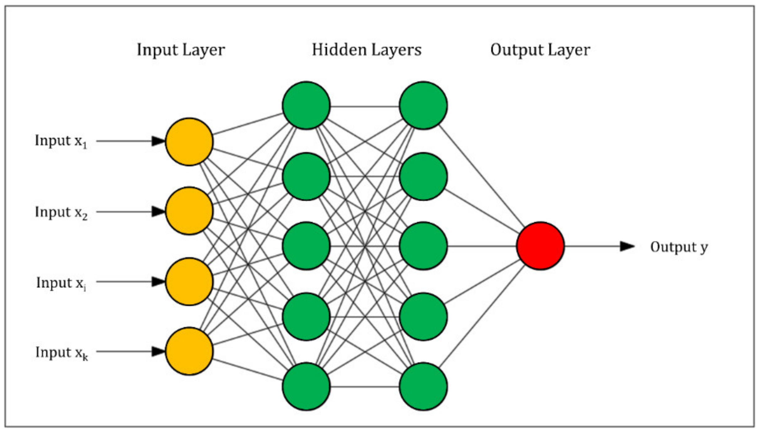
A Multilayer Perceptron (MLP) is a simple feedforward Artificial Neural Network [38]. An MLP (Figure 1) includes three types of layers: an input layer, one or more hidden layers, and an output layer. The input layer comprises a set of nodes corresponding to the input features. Each neuron in the hidden layers processes the values of the previous layer with a weighted linear summation, followed by a non-linear activation function. The output layer obtains the values from the last hidden layer and provides the output values. The neurons in the MLP are trained with the supervised technique called back propagation learning algorithm. Based on a set of features and a target, MLP can train a non-linear function to execute regression operations.
In this research, the optimal structures of the neural networks had only one hidden layer, whose number of neurons was equal to (number of input variables + 1)/2. Sigmoid was chosen as activation function. The adopted learning rate was 0.3, while the selected momentum rate for the backpropagation algorithm was 0.2. A preliminary sensitivity analysis has shown that the model is not very sensitive to parameter variations.
2.1.2. Random Forest
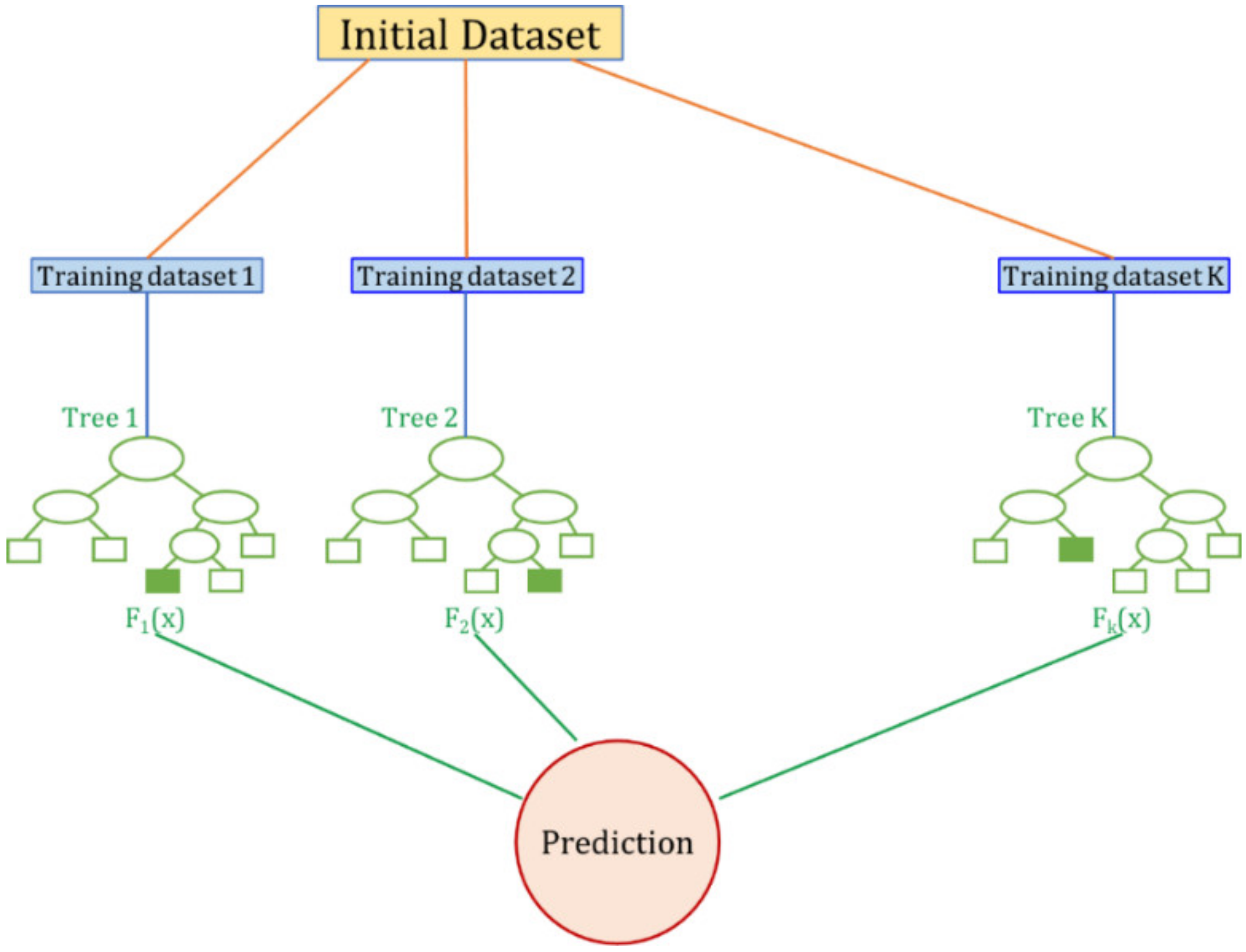
A Random Forest (Figure 2) is an ensemble model consisting of many uncorrelated, simple regression trees [39]. Regression Trees derive from decision trees adapted to become forecasting models [40]. The internal nodes progressively define conditions in the input variables, while leaves represent the target variables. Developing a regression tree model is a process that involves recursively splitting the input domain data into subdomains. A multivariable linear regression model is used to achieve predictions in each subdomain.
The tree growth is an iterative procedure, which progresses by splitting each subset into smaller branches, assessing all the possible splits on every field, and determining at each step the subdivision into two separate partitions that leads to the minimum squared deviation:
where N(t) is the sample size in the node t, yi is the value of the target variable in the i-th unit, while ym is the average value of the target variable in the node t. R(t) represents a measure of the “impurity” at each node. The algorithm stops when a halt condition occurs. Reaching the lowest level of impurity is the most commonly used stopping rule.
The risk of overfitting is reduced by means of a pruning process, that decreases the size of the tree model by removing the splits that do not significantly improve the forecasting ability.
Based on a training dataset, each tree of the forest is built from a different bootstrap sample of the data. Furthermore, in Random Forests the growth process of a single tree is different, since each node is assigned not by referring to the best subdivision among all the input variables but by randomly choosing only a part of the variables to subdivide. The number of these variables does not change during the expansion of the forest. Each tree grows as much as possible, bound only by the assigned number of elements for each leaf, without pruning. The random forests used in this research were made of 600 trees.
2.1.3. Support Vector Regression
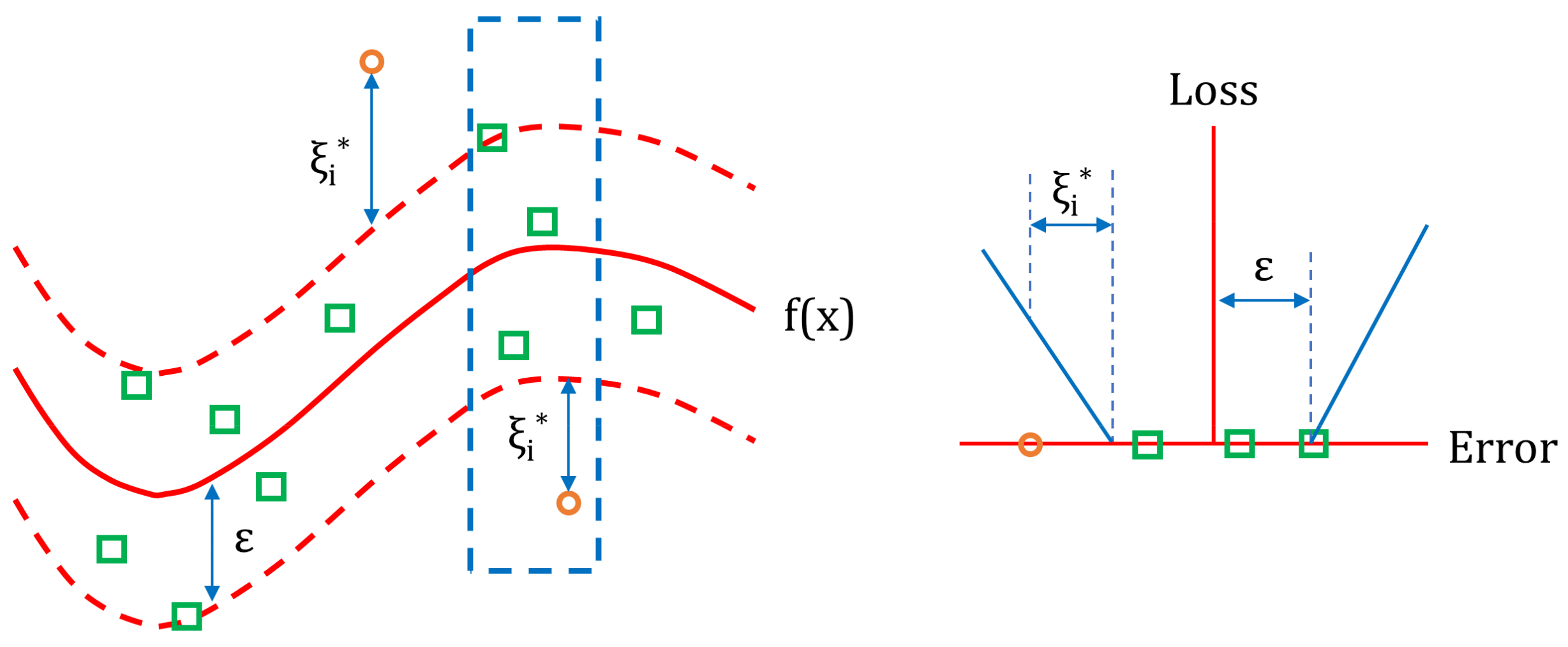
The idea behind the Support Vector Regression (SVR) algorithm is to identify a function f(x) with a maximum ε deviation from the experimental target values yi, and as flat as possible (Figure 3). Starting from a training dataset {(x1, y1), (x2, y2), …, (xl, yl)} ⊂ X × R, where X is the space of the input arrays (e.g., X ∈ Rn), and a linear function:
where ∈ X and b ∈ R, the Euclidean norm ||w||2 needs to be minimized. This involves the solution of a constrained convex optimization problem.
In many cases it is necessary to accept a not very small error, thus slack variables ξι, ξι* need to be introduced in the constraints. Consequently, the optimization problem can be presented as follows:
where the flatness of the function and the accepted deviations depend on the constant C > 0.
In order to make the SVR algorithm on linear, the training instances xi are pre-processed by a function Φ: X→F, where F is some feature space. Since SVR only depends on the dot products between the different instances, a kernel is used rather than explicitly employing the function Φ(∙).
In this study, the Pearson VII universal function kernel (PUFK) has been chosen:
where the parameters σ and ω affect the half-width and the tailing factor of the peak. The optimal results have been obtained for σ = 0.5, ω = 0.5. Based on preliminary analyzes, it was found that the PUK function led to more accurate predictions than possible alternatives such as Radial Basis Function, Polynomial, or Sigmoid.
2.2. Hybrid Models and Evaluation Metrics
Based on the predictions obtained with the different algorithms, it is possible to develop hybrid models by combining conceptually different machine learning regressors to improve the modelling performances. A framework for the different rules for the combination of classifiers was given by Kittler et al. [41].
In this research the different regressors were combined using the average probabilities approach to obtain the final prediction. This approach, also known as soft voting, can be useful for a set of similarly performing models in order to balance out their individual weaknesses.
Individual models were optimized using a random search procedure. The values of the parameters adopted in the individual algorithms, i.e., MLP, Random Forest and SVM, within the hybrid model, were the same as reported in the previous sections.
Four different metrics were used to assess the effectiveness of the prediction models: the Coefficient of Determination R2, the Mean Absolute Error (MAE), the Root Mean Squared Error (RMSE), and the Relative Absolute Error (RAE).
R2 indicates the proportional amount of variation in the response variable explained by the independent variables. It assesses how the model fits observed results and how well it forecasts future outcomes, providing very good assessment of the model accuracy.
MAE evaluates the average magnitude of the errors in a set of predictions, without considering their direction.
RMSE is the sample standard deviation of the residuals. It measures the data concentration around the best-fit line.
RAE evaluates a normalized total absolute error. These performance metrics are defined as follows:
where m is the total number of observed data, fi is the predicted value for data point i, yi is the measured value for data point i, and ya is the averaged value of the observed data. The use of the four metrics defined above allows full characterization of the accuracy of the forecast models developed, as they measure the goodness of fit, absolute, and relative errors.
2.3. Training Dataset
The data used for the modelling were extracted from the Soil Water Infiltration Global (SWIG) database [42], a global database of soil infiltration measurements that also provides some Ksat values. SWIG database includes data from 54 different countries, with major contributions from China, Iran, and the USA, collected from 1976 to 2017. Records were extracted from the dataset considering only the cases that included all the variables of interest for this study. Here the fraction of Clay, Silt and Sand, the mean and standard deviation of soil particle diameter, the soil organic carbon content, the soil bulk density, and the saturated soil water content have been considered, insofar as a large part of data was discarded from the entire dataset. A complete statistical description of the assumed dataset, divided by texture classes, is reported in Table 1 and Table 2. The two tables are separated only for layout reasons. For each texture and for each characteristic of interest, the tables show the minimum, maximum and median values, the first and third quartile, mean, standard deviation, and skewness of the distribution. In the tables, data are grouped considering the main soil component.
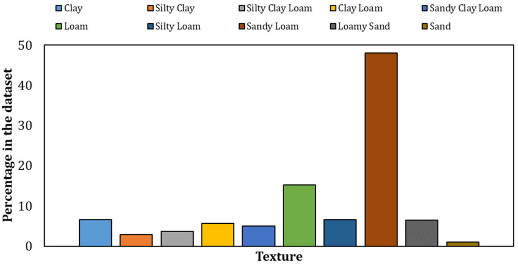
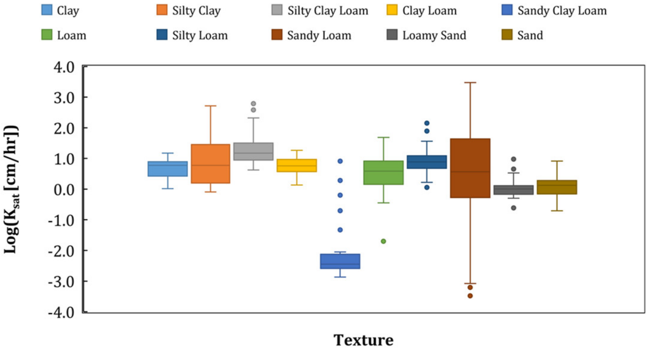
The characterization of the training dataset is completed by Figure 4 and Figure 5. Figure 4 shows the training dataset composition with reference to soil texture. It can be noted that sandy loams represent by far the most prevalent type of soil, constituting almost 50% of the soils included in the dataset. Figure 5 shows hydraulic conductivity box plots for the different types of soil. It can be noted that all types have a rather limited variability of conductivity, except for sandy loams. Moreover, few data records are characterized by the conductivity range 10−3 < Ksat < 10−2 cm/h. These fall almost exclusively into the sandy clay loams.
3. Results
Based on different combinations of input variables, five models were built for the prediction of Ksat. Seven variants of each model were developed, changing the implemented machine learning algorithm. Model M1 is characterized by the following input variables: the Clay percentage, the Silt percentage, the Sand percentage, the geometric mean diameter dg (mm), the standard deviation of soil particle diameter Sg, the soil organic carbon content OC (%), the soil bulk density Db (g/cm3), and the saturated soil water content WCs (g/g).
Model M2 needs the following input variables: dg, Sg, OC, Db, and WCs. Model M3 requires as input the following quantities: dg, Sg, Db, and WCs. The M4 model is based on dg, Sg, OC, and Db. Finally, the simplest model, M5, requires only dg, Sg, and Db as input variables.
Each model was built through a k-fold cross validation procedure [43], using a set of 640 vectors. In k-fold cross validation, the initial dataset is randomly partitioned into k subsets. Then, k − 1 subsets are employed as training data while the remaining single subset is used as the validation data. The cross-validation process is repeated k times: every subset is used once as the validation dataset. Finally, the k results from the folds are averaged to provide a single outcome. In this study k = 20 led to optimal results. In order to improve the performance of model training, the input data underwent a normalization process (min-max feature scaling), to bring all values into the range [0, 1].
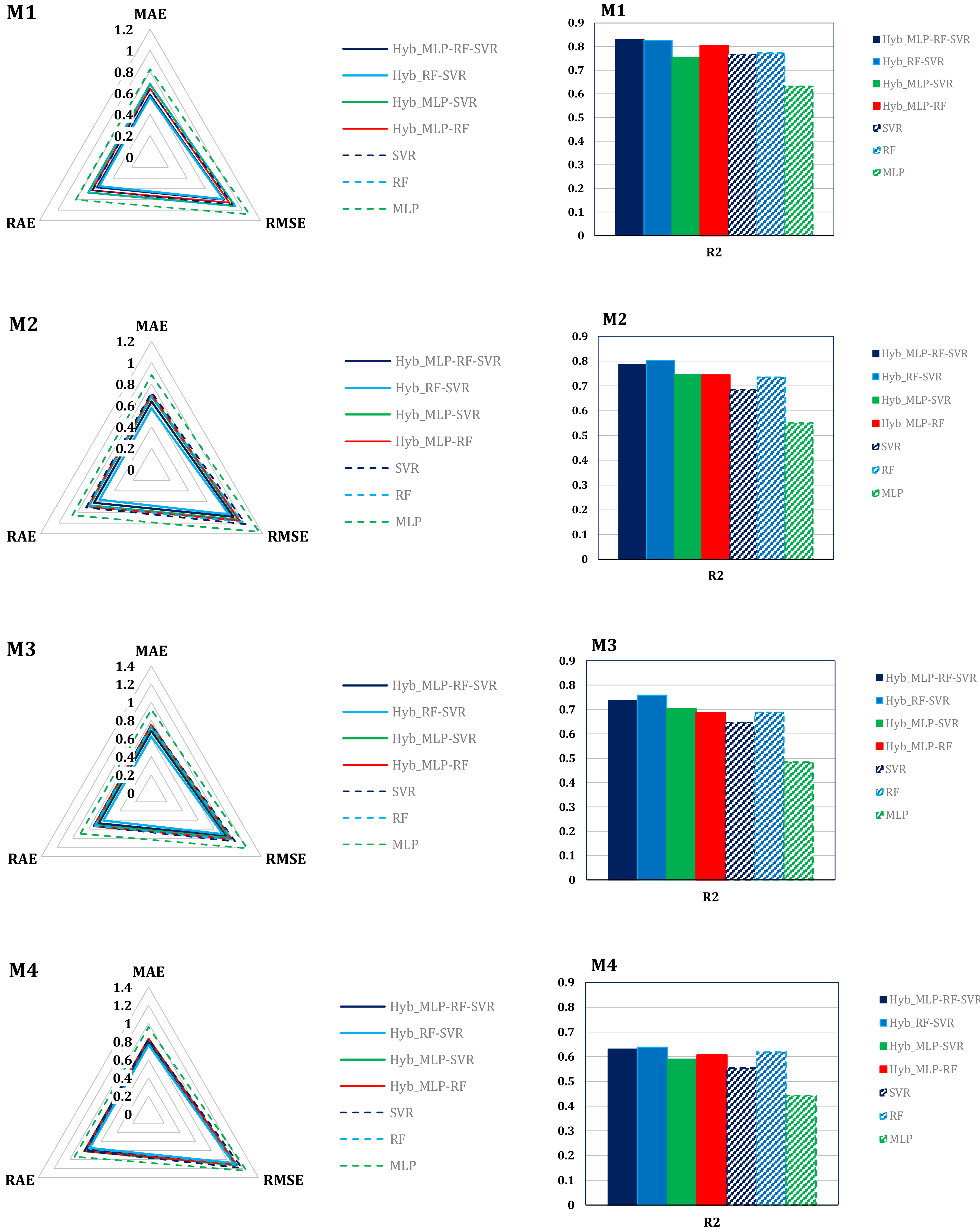
Model M1 showed the best predictive capabilities. The hybrid models Hyb_MLP-RF-SVR (R2 = 0.829, MAE = 0.582 log10 (cm/h), RMSE = 0.802 log10 (cm/h), RAE = 57.19%) and Hyb_RF-SVR (R2 = 0.826, MAE = 0.562 log10 (cm/h), RMSE = 0.796 log10 (cm/h), RAE = 55.16%) led to the best outcomes. The two hybrid models Hyb_MLP-RF and Hyb_MLP-SVR showed forecasting capabilities comparable to those of the two models based on RF and VR. The MLP-based model was by far the least accurate (R2 = 0.632, MAE = 0.821 log10 (cm/h), RMSE = 1.079 log10 (cm/h), RAE = 80.63%).
Model M2 underperformed M1 in all its variants. In this case, Hyb_RF-SVR clearly outperformed the other variants. The Hyb_MLP-RF-SVR variant was more accurate than the other two hybrid variants, Hyb_MLP-SVR and Hyb_MLP-RF, while these in turn outperformed RF, SVR, and MLP.
The M3 model showed a further reduction in prediction accuracy, in all variants. The Hyb_RF-SVR variant again proved to be the best performing model (R2 = 0.759, MAE = 0.622 log10 (cm/h), RMSE = 0.910 log10 (cm/h), RAE = 61.04%). The hybrid models once again proved more accurate than the basic models, except for the Hyb_MLP-RF model (R2 = 0.687, MAE = 0.749 log10 (cm/h), RMSE = 1.026 log10 (cm/h), RAE = 73.65%), whose results were barely less accurate than the results provided by RF.
The accuracy of the M4 model was unsatisfactory. The Hyb_RF-SVR variant also, in this case, led to the best predictions, but the superiority of the hybrid models was not as clear as in the case of the M1 and M2 models; indeed, RF outperformed both Hyb_MLP-RF and Hyb_MLP-SVR.
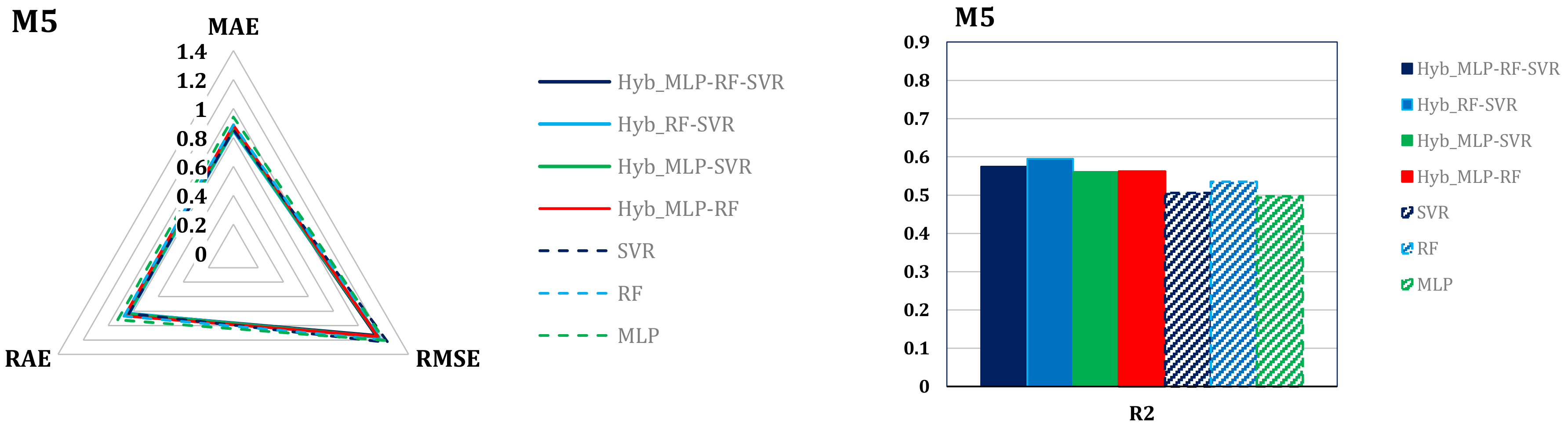
The M5 model led to somewhat poor results. Even the most accurate of the variants, again represented by Hyb_RF-SVR, was characterized by unsatisfactory values of the efficiency metrics (R2 = 0.595, MAE = 0.848 log10 (cm/h), RMSE = 1.164 log10 (cm/h), RAE = 83.37%).
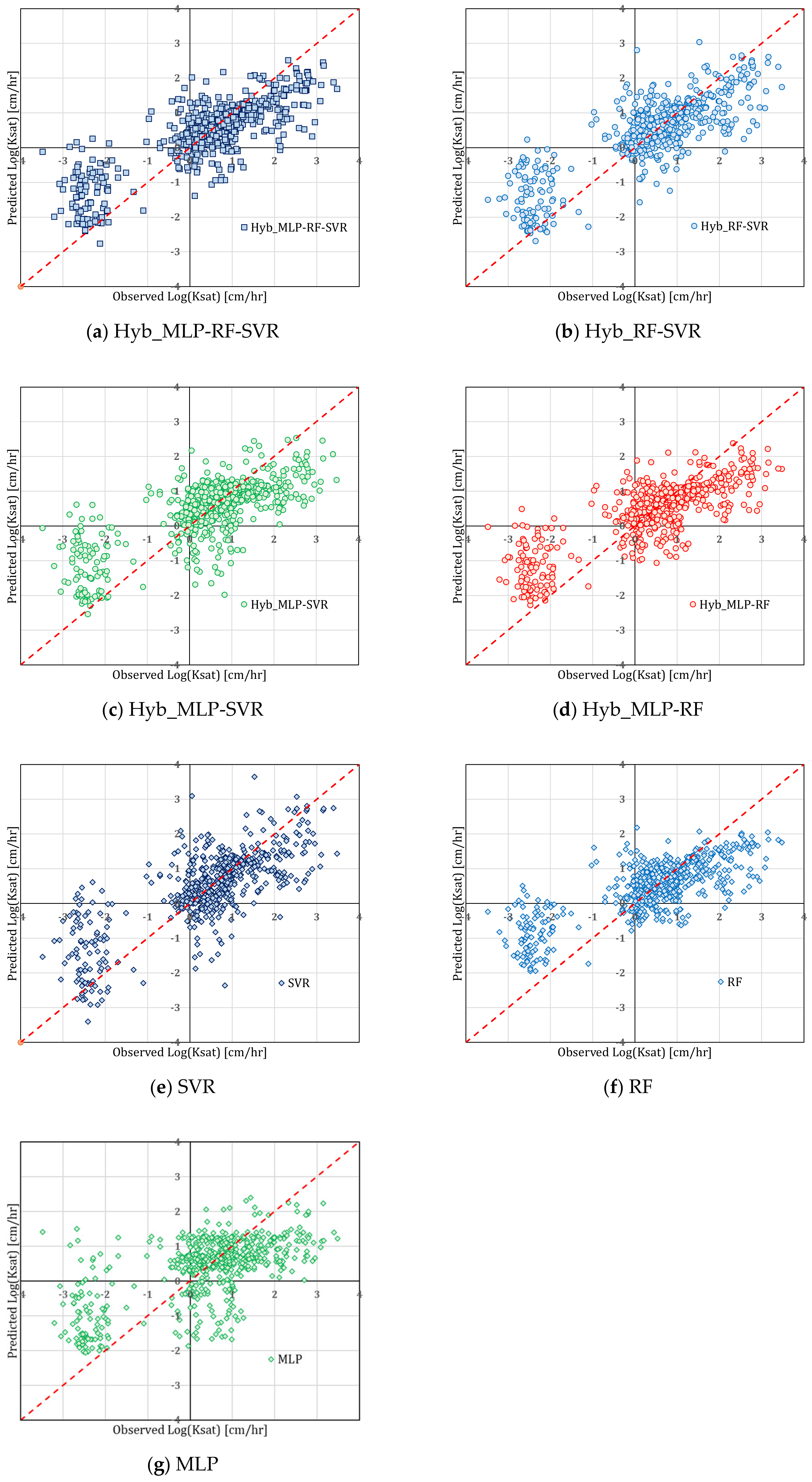
Figure 7, which reports the predicted values versus the observed values for the M1 model, shows that all variants have had better accuracy in the range 100 < Ksat <102 cm/h. Likewise, all variants showed a tendency to overestimate Ksat in the range 10−3 < Ksat < 10−2 cm/h. The reason for this unsatisfactory result lies both in the more limited number of training data falling within this interval, and in the greater heterogeneity of the same as regards the values of the predictors. This trend also characterized the other models with worse performances. The diagrams have not been reported for the sake of brevity.
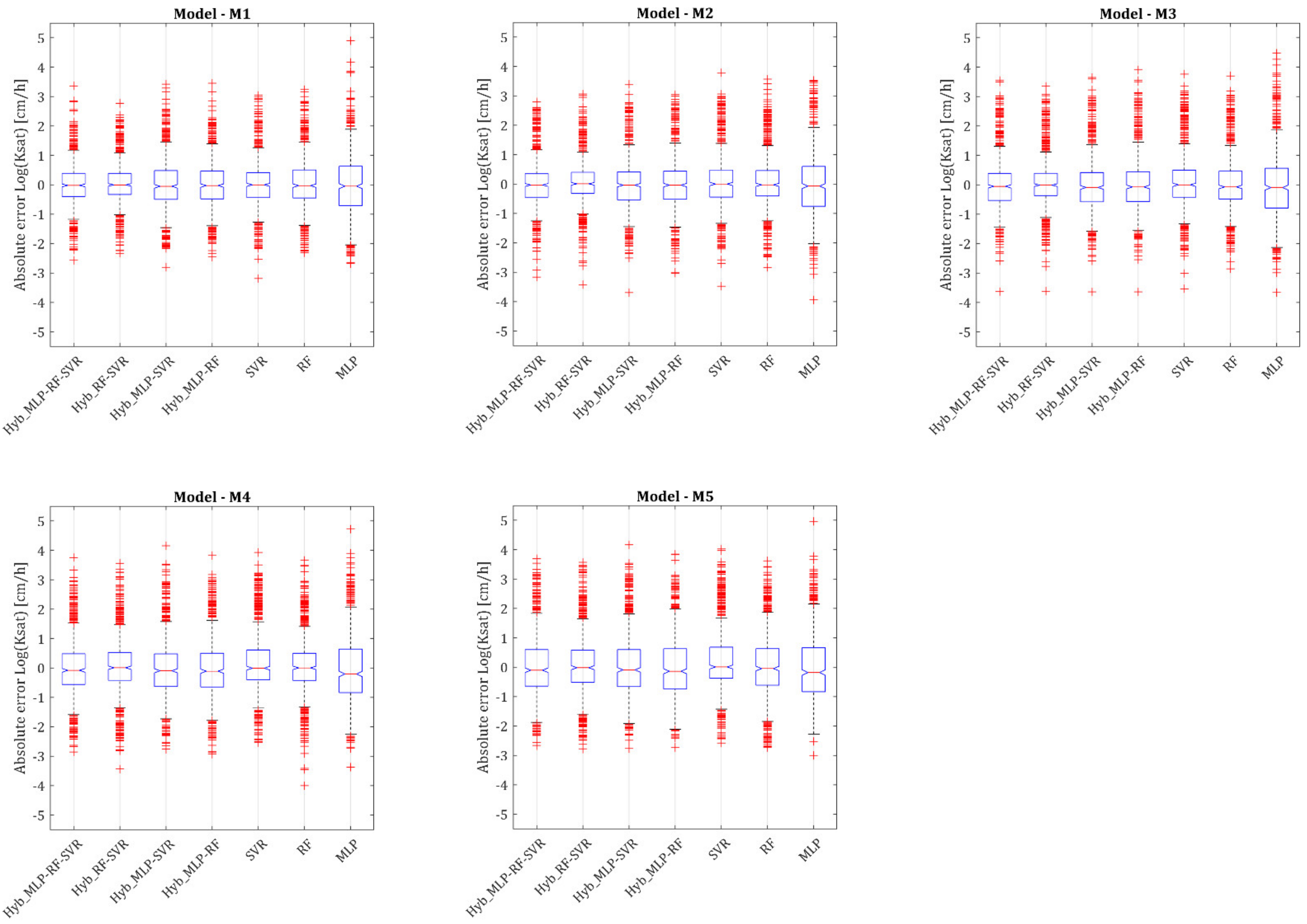
From the graphs of Figure 8, which show the box plots of the absolute errors = predicted values—actual values, the following can be deduced:
- -
- All variants of the M1 and M2 models have a negligible bias. A more appreciable, albeit slight bias is observed in the SVR and MLP based variants of the M4 and M5 models.
- -
- The Hyb_MLP-RF-SVR and Hyb_RF-SVR variants are characterized by the lowest variance of the absolute error within all the considered models, in particular within the M1 and M2 models.
- -
- Model M1 shows the lowest number of outliers.
- -
- The distribution of the error in all variants of the M3, M4, and especially M5 models, is clearly asymmetrical.
These results help to better understand the above in terms of metrics analysis.
In order to further highlight the effectiveness of the approach based on machine learning algorithms, a comparison with a classic formulation for the estimation of Ksat is proposed below. The prediction with theoretical, empirical or semi-empirical equations that relate the saturated conductivity coefficient of porous materials to physical properties of the seeping fluid and soil assembly is a classical goal of research. Starting from the Hagen–Poiseuille equation that describes the flow of a fluid in capillary pipes, the Kozeny–Carman equation [7,44] is among the first written equations:
where ρw and μw are respectively the density and viscosity of water (set equal to ρw = 1000 kg/m3; μw = 0.001 Pa*s)), g is gravity, n is the soil porosity, and So is the surface of soil particles per unit volume. Alternatively, the equation can be expressed as:
where e is the void ratio (=n/(1 − n)), Dg is geometric mean particle size, obtained by subdividing the grain size distribution into l classes and computing:
where fi and di are respectively the fraction of contained material and the representative diameter of each class. The coefficient C (equal generally to 180) can be particularized including a dependency on the particle shapes expressed by a sphericity factor. Carman [8] and other researchers showed that this equation is quite effective in estimating permeability for coarse-grained soils.
On the other hand, experimental evidence does not confirm the validity of this relationship for clay soils. Taylor [45] ascribed this difference to the reduction in the effective pore space available for the free flow of fluid due to the film of water attached to the surfaces of clay particles. Olsen [46] considered the difference between water conductivity measured in saturated clay and the values predicted with the Kozeny-Carman relation to the heterogenous pore size distribution of clay materials. Chapuis and Aubertin [47] adopted the Specific Surface Area to predict the vertical permeability coefficient of a homogeneous soil. Ren et al. [48] introduced the concept of effective void ratio subdividing the total volume of voids into two parts, one effective ee occupied by flowing water, the other ineffective ei occupied by immobile water, i.e., attached to the soil particles of located closed pores. These authors proposed the following relation between effective and total void ratio:
where m is a non-negative constant ranging between 0 and 2 (m = 0.05 ± 0.05 for sandy soil, m = 1 ± 0.2 for silty soil, m = 1.5 ± 0.5 for clay).
In the present work, the permeability coefficient has been computed with the following formula extracted from Hong et al. (2020):
Considering the available database, ρs has been fixed as equal to 2650 kg/m3, the effective void ratio ee has been computed with Equation (13), setting the exponent m equal to 1.5, i.e., considering the relevant presence in each dataset of silt and clay components; the ineffective void ratio has been computed as ei = e − ee. The specific surface So has been evaluated as function of the clay fraction, adopting the mean curve among the data collected by Hong et al. [49].
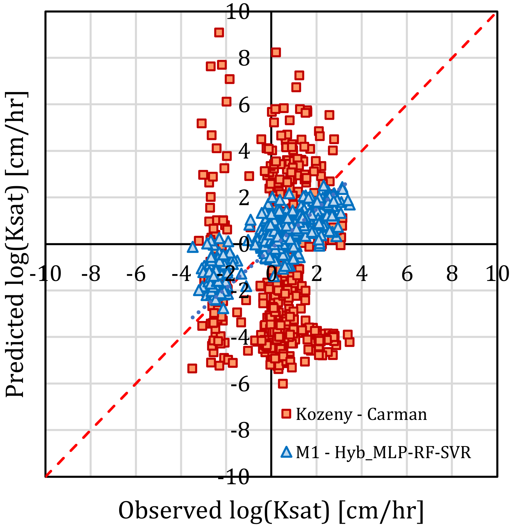
The comparison between the results obtained with the M1 model, Hyb_MLP-RF-SVR variant, and those obtained with the Kozeny-Carman formulation is shown in Figure 9. For the predictions obtained with the Kozeny-Carman equation, the following values of the metrics considered above were found: R2 = 0.187, MAE = 3.52 log10 (cm/h), RMSE = 6.23 log10 (cm/h), RAE = 346%). It is quite evident that an approach based on machine learning algorithms is significantly more effective than a classic approach based on formulations deriving from the studies of Kozeny, Carman, and subsequently. The better performance justifies the greater complexity of the forecasting tool.
4. Discussion
The combination of the different predictors is of considerable importance to the accuracy of Ksat estimate based on the physical characteristics of soil. It is essential that the number of input variables is sufficiently representative of the soil characteristics. The detailed knowledge of the soil grain size distribution, and particularly of the fractions of clay, silt, and sand, together with the mean and standard deviation of soil particle diameter, is a fundamental starting point for a Ksat prediction with machine learning algorithms. However, some preliminary analyses have shown that the parameters obtainable from the grain size distribution curve alone do not enable a sufficiently accurate model, therefore the relative results have not been shown here. Knowledge of additional parameters such as the soil organic content, bulk density, and the saturated soil water content is essential to improve the accuracy of predicting models. Similarly, models based only on global geometric parameters such as dg, Sg, and Db fail to provide acceptable results.
Hybrid models have appreciably outperformed individual base models in predicting Ksat in the more complex cases of models characterized by a greater number of predictors (e.g., M1 and M2). This result agrees with those obtained by other scholars in the context of relevant scientific contributions on other topics. Pham and Prakash [50] proposed a novel use of bagging-based naïve Bayes trees for the assessment of landslide susceptibility. The developed hybrid model was compared to individual models including Rotation forest-based Naïve Bayes Trees, Naïve Bayes Trees, and SVM. The hybrid method proved to be the most accurate model for the assessment of landslide vulnerability, increasing the accuracy of the standalone models. Wu et al. [51] proposed a hybrid model to forecast electricity load in five states of Australia. The developed model included an advanced integration of Extreme Learning Machine, ensemble empirical mode decomposition, and grasshopper optimization algorithm. The hybrid model was compared to some base models in terms of RMSE, MAE and Mean Absolute Percentage Error (MAPE), showing a higher performance and accuracy. Bui et al. [52] used four individual (random forest, M5P, random tree, and reduced error pruning tree) and 12 hybrid ML algorithms to predict water quality indices in a humid catchment of northern Iran. The results of the hybrid models, compared to the individual algorithms, showed that they had improved prediction accuracies, but may not be as successful in all cases.
The above-mentioned literature shows that hybrid methods are becoming more and more popular due capability in improving prediction performance. Hybrid machine learning leads to the best performance when the underlying models are not correlated. For instance, it is possible to train different models such as regression trees, neural network, and support vector machines on different datasets or features. The less correlated the base models are, the better the forecasting performance. The idea behind using uncorrelated models is that each could address a weakness in the other. They also have different strengths which, when combined, will result in a good performing estimator.
Despite the much smaller size of the training dataset, and the smaller number of considered predictors, the predictive ability of the hybrid models developed in this study is close to that of the best models developed by Araya and Ghezzehei [35]. A further comparison with Jorda et al. [34] and Kotlar et al. [36] supports even further the need to train the models with large and varied datasets; otherwise, accuracy of prediction may become unsatisfactory. This aspect might be seen as a main weakness of this study: a too broad classification of the soil types, mostly for those characterized by a very low conductivity, had a significant negative impact on the overall performance of the model. Additionally, the insufficient size of the training dataset for some soil categories might play a negative role too, as well as the predominant presence of data relating to sandy loam samples in the initial dataset. Another factor that negatively affects the performance of prediction is the heterogeneity of the training dataset. Permeability coefficients have been obtained under very different experimental conditions, generally aimed at evaluating the infiltration rate. This variety introduces a considerable noise into the estimate of Ksat as shown by the large variability of results within each soil category. However, the above factors, out of control in the present analysis, negatively impact on the training and performance of any predictive model. In the authors’ opinion, the interpretation of dependencies inherent in the proposed model might serve also to create new databases with a more coherent categorization of soil types, and to the more appropriate definition of relevant variables. In addition, the availability in the future of a dataset as homogeneous as possible as regards the Ksat estimation method represents a necessary condition for obtaining significant improvements in the forecasting capabilities of models based on Machine Learning algorithms.
Future developments of this research will be aimed at further improving the accuracy of forecasting models, especially for soils characterized by low hydraulic conductivity, considering larger and more varied training datasets, a greater number of predictors and hybridizing different basic algorithms. In addition, it could be useful to develop different predictive models for coarse-grained and fine-grained soils, given the considerable differences in the seepage processes observed in them.
5. Conclusions
An accurate prediction of the hydraulic conductivity of a saturated soil is essential to address groundwater issues. If reliable data are available, machine learning algorithms are powerful tools to obtain good predictions. In addition, hybrid models resulting from the combination of multiple machine learning algorithms can further improve the performance of individual models.
In this study, five different models were developed to predict saturated hydraulic conductivity starting from a dataset extracted from the Soil Water Infiltration Global database. The models differed in the input variables. Seven variants of each model were compared, changing the employed algorithm. Three variants were based on individual models, while four variants were based on hybrid models. The selected individual machine learning algorithms were Multilayer Perceptron, Random Forest, and Support Vector Regression.
Model M1, which requires as input variables the clay percentage, the silt percentage, the sand percentage, the geometric mean diameter, the standard deviation of soil particle diameter, the soil organic carbon content, the soil bulk density, and the saturated soil water content, led to the most accurate results. The M4 and M5 models, based on a limited number of soil characteristics, gave unsatisfactory results.
Across all models, hybrid variants based on all three algorithms and hybridized variants of Random Forest and Support Vector Regression provided the most accurate predictions. However, all variants showed a tendency to overestimate Ksat in the range 10−3 < Ksat < 10−2 cm/h, due to the reduced number of training data falling within this interval, and in the high heterogeneity of the same data as concerns the values of the predictors.
A comparison with the classic Kozeny-Carman formulation further demonstrated the convenience of an approach based on machine learning algorithms, given the significantly higher performance.
Author Contributions
F.G.: Conceptualization, data curation, formal analysis, methodology, software, supervision, writing—original draft, writing—review and editing; F.D.N.: conceptualization, methodology, writing—original draft, writing—review and editing; G.M.: conceptualization, methodology, writing—original draft, writing—review and editing. All authors have read and agreed to the published version of the manuscript.
Funding
This research received no external funding.
Institutional Review Board Statement
Not applicable.
Informed Consent Statement
Not applicable.
Data Availability Statement
The datasets generated and analysed during the current study are available in the repository: https://doi.pangaea.de/10.1594/PANGAEA.885492 (last accessed on 31 March 2022).
Conflicts of Interest
The authors declare that they have no competing interests.
References
- Adamowski, J.; Chan, H.F. A wavelet neural network conjunction model for groundwater level forecasting. J. Hydrol. 2011, 407, 28–40. [Google Scholar] [CrossRef]
- Alamanis, N.; Papageorgiou, G.; Chantzopoulou, P.; Chouliaras, I. Investigation on the influence of permeability coefficient k of the soil mass on construction settlements. Cases of infrastructure settlements in Greece. Wseas Trans. Environ. Dev. 2019, 15, 95–105. [Google Scholar]
- Alyamani, M.S.; Şen, Z. Determination of hydraulic conductivity from complete grain-size distribution curves. Groundwater 1993, 31, 551–555. [Google Scholar] [CrossRef]
- Angelaki, A.; Singh Nain, S.; Singh, V.; Sihag, P. Estimation of models for cumulative infiltration of soil using machine learning methods. ISH J. Hydraul. Eng. 2021, 27, 162–169. [Google Scholar] [CrossRef]
- Araya, S.N.; Ghezzehei, T.A. Using machine learning for prediction of saturated hydraulic conductivity and its sensitivity to soil structural perturbations. Water Resour. Res. 2019, 55, 5715–5737. [Google Scholar] [CrossRef]
- Azamathulla, H.M.; Wu, F.C. Support vector machine approach for longitudinal dispersion coefficients in natural streams. Appl. Soft Comput. 2011, 11, 2902–2905. [Google Scholar] [CrossRef]
- Boadu, F.K. Hydraulic conductivity of soils from grain-size distribution: New models. J. Geotech. Geoenviron. Eng. 2000, 126, 739–746. [Google Scholar] [CrossRef]
- Breiman, L. Random forests. Mach. Learn. 2001, 45, 5–32. [Google Scholar] [CrossRef] [Green Version]
- Breiman, L.; Friedman, J.H.; Olshen, R.A.; Stone, C.J. Classification and Regression Trees; Routledge: Abingdon, UK, 2017. [Google Scholar]
- Bui, D.T.; Khosravi, K.; Tiefenbacher, J.; Nguyen, H.; Kazakis, N. Improving prediction of water quality indices using novel hybrid machine-learning algorithms. Sci. Total Environ. 2020, 721, 137612. [Google Scholar] [CrossRef]
- Carman, P.C. Permeability of saturated sands, soils and clays. J. Agric. Sci. 1939, 29, 263–273. [Google Scholar] [CrossRef]
- Carman, P.C. Flow of Gas through Porous Media; Butterworths Scientific Publications: London, UK, 1956. [Google Scholar]
- Chapuis, R.P. Predicting the saturated hydraulic conductivity of soils: A review. Bull. Eng. Geol. Environ. 2012, 71, 401–434. [Google Scholar] [CrossRef]
- Chapuis, R.P.; Aubertin, M. On the use of the Kozeny Carman equation to predict the hydraulic conductivity of soils. Can. Geotech. J. 2003, 40, 616–628. [Google Scholar] [CrossRef]
- Crawford, J.W. The relationship between structure and the hydraulic conductivity of soil. Eur. J. Soil Sci. 1994, 45, 493–502. [Google Scholar] [CrossRef]
- Di Nunno, F.; Granata, F. Groundwater level prediction in Apulia region (Southern Italy) using NARX neural network. Environ. Res. 2020, 190, 110062. [Google Scholar] [CrossRef] [PubMed]
- Freeze, R.A.; Cherry, J.A. Groundwater; Prentice Hall Inc.: Hoboken, NJ, USA, 1979. [Google Scholar]
- Fushiki, T. Estimation of prediction error by using K-fold cross-validation. Stat. Comput. 2011, 21, 137–146. [Google Scholar] [CrossRef]
- Granata, F. Evapotranspiration evaluation models based on machine learning algorithms—A comparative study. Agric. Water Manag. 2019, 217, 303–315. [Google Scholar] [CrossRef]
- Granata, F.; Di Nunno, F. Artificial Intelligence models for prediction of the tide level in Venice. Stoch. Environ. Res. Risk Assess. 2021, 35, 2537–2548. [Google Scholar] [CrossRef]
- Granata, F.; Di Nunno, F. Forecasting evapotranspiration in different climates using ensembles of recurrent neural networks. Agric. Water Manag. 2021, 255, 107040. [Google Scholar] [CrossRef]
- Han, H.; Giménez, D.; Lilly, A. Textural averages of saturated soil hydraulic conductivity predicted from water retention data. Geoderma 2008, 146, 121–128. [Google Scholar] [CrossRef]
- Haykin, S. Neural Networks: A Comprehensive Foundation; Prentice Hall Inc.: Hoboken, NJ, USA, 1994. [Google Scholar]
- Hu, W.; She, D.; Shao, M.; Chun, K.P.; Si, B. Effects of initial soil water content and saturated hydraulic conductivity variability on small watershed runoff simulation using LISEM. Hydrol. Sci. J. 2015, 60, 1137–1154. [Google Scholar] [CrossRef]
- Hong, B.; Li, X.A.; Wang, L.; Li, L.; Xue, Q.; Meng, J. Using the effective void ratio and specific surface area in the Kozeny–Carman equation to predict the hydraulic conductivity of loess. Water 2020, 12, 24. [Google Scholar] [CrossRef] [Green Version]
- Jabro, J.D. Estimation of saturated hydraulic conductivity of soils from particle size distribution and bulk density data. Trans. ASAE 1992, 35, 557–560. [Google Scholar] [CrossRef]
- Jorda, H.; Bechtold, M.; Jarvis, N.; Koestel, J. Using boosted regression trees to explore key factors controlling saturated and near-saturated hydraulic conductivity. Eur. J. Soil Sci. 2015, 66, 744–756. [Google Scholar] [CrossRef]
- Kişi, Ö. Streamflow forecasting using different artificial neural network algorithms. J. Hydrol. Eng. 2007, 12, 532–539. [Google Scholar] [CrossRef]
- Kittler, J.; Hatef, M.; Duin, R.P.W.; Matas, J. On Combining Classifiers. IEEE Trans. Pattern Anal. Mach. Intell. 1998, 20, 226–239. [Google Scholar] [CrossRef] [Green Version]
- Knoll, L.; Breuer, L.; Bach, M. Large scale prediction of groundwater nitrate concentrations from spatial data using machine learning. Sci. Total Environ. 2019, 668, 1317–1327. [Google Scholar] [CrossRef]
- Kotlar, A.M.; Iversen, B.V.; de Jong van Lier, Q. Evaluation of parametric and nonparametric machine-learning techniques for prediction of saturated and near-saturated hydraulic conductivity. Vadose Zone J. 2019, 18, 1–13. [Google Scholar] [CrossRef]
- Kozeny, J. Ueber kapillare Leitung des Wassers im Boden. Sitzungsberichte Wiener Akademie 1927, 136, 271–306. [Google Scholar]
- Kumar, M.; Sihag, P. Assessment of infiltration rate of soil using empirical and machine learning-based models. Irrig. Drain. 2019, 68, 588–601. [Google Scholar] [CrossRef]
- Modoni, G.; Darini, G.; Spacagna, R.L.; Saroli, M.; Russo, G.; Croce, P. Spatial analysis of subsidence induced by groundwater withdrawal. Eng. Geol. 2013, 167, 59–71. [Google Scholar] [CrossRef]
- Montzka, C.; Herbst, M.; Weihermüller, L.; Verhoef, A.; Vereecken, H. A global data set of soil hydraulic properties and sub-grid variability of soil water retention and hydraulic conductivity curves. Earth Syst. Sci. Data 2017, 9, 529–543. [Google Scholar] [CrossRef] [Green Version]
- Najafzadeh, M.; Etemad-Shahidi, A.; Lim, S.Y. Scour prediction in long contractions using ANFIS and SVM. Ocean Eng. 2016, 111, 128–135. [Google Scholar] [CrossRef]
- Najafzadeh, M.; Oliveto, G. Riprap incipient motion for overtopping flows with machine learning models. J. Hydroinform. 2020, 22, 749–767. [Google Scholar] [CrossRef]
- Odong, J. Evaluation of empirical formulae for determination of hydraulic conductivity based on grain-size analysis. J. Am. Sci. 2007, 3, 54–60. [Google Scholar]
- Olsen, H.W. Hydraulic flow through saturated clays. In Clays Clay Miner; Ingerson, E., Ed.; Elsevier: Amsterdam, The Netherlands, 1962; pp. 131–161. [Google Scholar]
- Pham, B.T.; Prakash, I. A novel hybrid model of bagging-based naïve bayes trees for landslide susceptibility assessment. Bull. Eng. Geol. Environ. 2019, 78, 1911–1925. [Google Scholar] [CrossRef]
- Rahmati, M.; Weihermüller, L.; Vanderborght, J.; Pachepsky, Y.A.; Mao, L.; Sadeghi, S.H.; Moosavi, N.; Kheirfam, H.; Montzka, C.; Van Looy, K.; et al. Development and analysis of the Soil Water Infiltration Global database. Earth Syst. Sci. Data 2018, 10, 1237–1263. [Google Scholar] [CrossRef] [Green Version]
- Ren, X.; Zhao, Y.; Deng, Q.; Kang, J.; Li, D.; Wang, D. A relation of hydraulic conductivity—Void ratio for soils based on Kozeny-Carman equation. Eng. Geol. 2016, 213, 89–97. [Google Scholar] [CrossRef]
- Saberi-Movahed, F.; Najafzadeh, M.; Mehrpooya, A. Receiving more accurate predictions for longitudinal dispersion coefficients in water pipelines: Training group method of data handling using extreme learning machine conceptions. Water Resour. Manag. 2020, 34, 529–561. [Google Scholar] [CrossRef]
- Sammen, S.S.; Ghorbani, M.A.; Malik, A.; Tikhamarine, Y.; AmirRahmani, M.; Al-Ansari, N.; Chau, K.W. Enhanced artificial neural network with Harris hawks optimization for predicting scour depth downstream of ski-jump spillway. Appl. Sci. 2020, 10, 5160. [Google Scholar] [CrossRef]
- Sihag, P.; Karimi, S.M.; Angelaki, A. Random forest, M5P and regression analysis to estimate the field unsaturated hydraulic conductivity. Appl. Water Sci. 2019, 9, 129. [Google Scholar] [CrossRef] [Green Version]
- Sihag, P.; Dursun, O.F.; Sammen, S.S.; Malik, A.; Chauhan, A. Prediction of aeration efficiency of parshall and modified venturi flumes: Application of soft computing versus regression models. Water Supply 2021, 21, 4068–4085. [Google Scholar] [CrossRef]
- Singh, U.K.; Jamei, M.; Karbasi, M.; Malik, A.; Pandey, M. Application of a modern multi-level ensemble approach for the estimation of critical shear stress in cohesive sediment mixture. J. Hydrol. 2022, 607, 127549. [Google Scholar] [CrossRef]
- Taylor, D.W. Fundamentals of Soil Mechanics; Wiley: New York, NY, USA, 1948; p. 12. [Google Scholar]
- Todd, D.K.; Mays, L.W. Groundwater Hydrology; Wiley: New York, NY, USA, 2004; p. 659. [Google Scholar]
- Wang, W.C.; Chau, K.W.; Cheng, C.T.; Qiu, L. A comparison of performance of several artificial intelligence methods for forecasting monthly discharge time series. J. Hydrol. 2009, 374, 294–306. [Google Scholar] [CrossRef] [Green Version]
- Woolhiser, D.A.; Smith, R.E.; Giraldez, J.V. Effects of spatial variability of saturated hydraulic conductivity on Hortonian overland flow. Water Resour. Res. 1996, 32, 671–678. [Google Scholar] [CrossRef]
- Wu, J.; Cui, Z.; Chen, Y.; Kong, D.; Wang, Y.G. A new hybrid model to predict the electrical load in five states of Australia. Energy 2019, 166, 598–609. [Google Scholar] [CrossRef]
Figure 1.
Typical structure of a Multilayer Perceptron.

Figure 2.
Typical architecture of the Random Forest algorithm.

Figure 3.
Example of Support Vector Regression. Errors can be neglected if they are less than ε, while larger deviations are penalized.
Figure 3.
Example of Support Vector Regression. Errors can be neglected if they are less than ε, while larger deviations are penalized.

Figure 4.
Training dataset composition with reference to soil texture.

Figure 5.
Hydraulic conductivity box plots for the different types of soil.

Figure 6.
Radar charts of the error metrics (left column) and histograms of the coefficients of determination (right column).
Figure 6.
Radar charts of the error metrics (left column) and histograms of the coefficients of determination (right column).


Figure 7.
Hydraulic conductivities predicted versus observed for the different variants of the M1 model.
Figure 7.
Hydraulic conductivities predicted versus observed for the different variants of the M1 model.

Figure 8.
Box plots of the absolute errors in all models and variants.

Figure 9.
Comparison between the results obtained with the M1 model, Hyb_MLP-RF-SVR variant, and those obtained with the Kozeny-Carman formulation.
Figure 9.
Comparison between the results obtained with the M1 model, Hyb_MLP-RF-SVR variant, and those obtained with the Kozeny-Carman formulation.


Table 1.
Characteristics of the training dataset (1/2).
| Clay | Silt | Sand | dg | Sg | OC | Db | WC_s | Log(Ksat) | ||
|---|---|---|---|---|---|---|---|---|---|---|
| [%] | [%] | [%] | [mm] | [%] | [g/cm3] | [cm3/cm3] | Log [cm/hr] | |||
| Clay | Minimum value | 40.40 | 9.0 | 4.60 | 0.002 | 6.147 | 0.650 | 0.461 | 0.217 | 0.014 |
| 1st Quartile | 48.500 | 35.0 | 9.525 | 0.005 | 9.339 | 3.413 | 0.754 | 0.326 | 0.423 | |
| Median | 51.000 | 37.3 | 11.7 | 0.007 | 10.383 | 4.350 | 0.977 | 0.397 | 0.777 | |
| 3rd Quartile | 55.800 | 38.8 | 15.375 | 0.009 | 11.914 | 6.230 | 1.101 | 0.481 | 0.892 | |
| Maximum value | 80.000 | 39.8 | 36.0 | 0.024 | 21.520 | 11.572 | 1.468 | 0.590 | 1.174 | |
| Mean | 53.557 | 33.661 | 12.777 | 0.008 | 10.846 | 5.212 | 0.963 | 0.402 | 0.668 | |
| Standard Deviation | 9.071 | 8.818 | 6.660 | 0.004 | 3.114 | 2.661 | 0.242 | 0.102 | 0.322 | |
| Skewness | 1.359 | −1.812 | 1.656 | 2.028 | 1.603 | 1.044 | 0.127 | 0.178 | −0.887 | |
| Silty Clay | Minimum value | 44.900 | 40.5 | 1.0 | 0.005 | 5.490 | 2.230 | 0.687 | 0.232 | −0.095 |
| 1st Quartile | 45.200 | 43.5 | 8.525 | 0.008 | 8.545 | 2.230 | 0.861 | 0.286 | 0.197 | |
| Median | 45.400 | 43.5 | 10.0 | 0.009 | 9.206 | 4.630 | 0.973 | 0.348 | 0.777 | |
| 3rd Quartile | 45.550 | 46.2 | 11.1 | 0.009 | 9.716 | 4.910 | 1.283 | 0.408 | 1.457 | |
| Maximum value | 55.800 | 46.4 | 13.5 | 0.010 | 10.849 | 8.680 | 1.580 | 0.471 | 2.718 | |
| Mean | 46.922 | 43.883 | 9.194 | 0.008 | 8.905 | 4.240 | 1.064 | 0.348 | 0.956 | |
| Standard Deviation | 3.833 | 2.130 | 3.357 | 0.002 | 1.424 | 2.053 | 0.268 | 0.074 | 0.859 | |
| Skewness | 1.976 | −0.329 | −1.180 | −1.618 | −1.016 | 0.927 | 0.348 | −0.073 | 0.638 | |
| Silty Clay Loam | Minimum value | 27.404 | 42.969 | 3.872 | 0.008 | 6.339 | 0.690 | 0.758 | 0.015 | 0.626 |
| 1st Quartile | 29.319 | 47.2 | 13.39 | 0.012 | 9.032 | 1.600 | 1.062 | 0.161 | 0.946 | |
| Median | 35.400 | 49.0 | 15.09 | 0.015 | 10.017 | 2.371 | 1.202 | 0.393 | 1.172 | |
| 3rd Quartile | 38.100 | 55.723 | 17.145 | 0.018 | 10.730 | 4.110 | 1.310 | 0.485 | 1.502 | |
| Maximum value | 39.651 | 63.734 | 19.70 | 0.020 | 12.421 | 6.780 | 1.476 | 0.549 | 2.787 | |
| Mean | 34.068 | 51.633 | 14.300 | 0.015 | 9.786 | 2.786 | 1.184 | 0.319 | 1.349 | |
| Standard Deviation | 4.398 | 6.164 | 4.446 | 0.003 | 1.800 | 1.590 | 0.190 | 0.187 | 0.592 | |
| Skewness | −0.387 | 0.326 | −1.147 | 0.065 | −0.623 | 0.763 | −0.353 | −0.421 | 1.199 | |
| Clay Loam | Minimum value | 27.003 | 21.926 | 20.70 | 0.016 | 11.302 | 0.577 | 0.617 | 0.030 | 0.134 |
| 1st Quartile | 29.000 | 39.575 | 23.0 | 0.019 | 13.122 | 2.165 | 0.982 | 0.356 | 0.572 | |
| Median | 30.600 | 40.5 | 25.95 | 0.024 | 13.728 | 3.045 | 1.173 | 0.433 | 0.759 | |
| 3rd Quartile | 34.830 | 44.029 | 30.800 | 0.031 | 14.638 | 3.570 | 1.406 | 0.538 | 0.969 | |
| Maximum value | 38.300 | 50.647 | 43.403 | 0.050 | 21.252 | 5.200 | 1.531 | 0.648 | 1.265 | |
| Mean | 31.971 | 40.888 | 27.141 | 0.026 | 14.110 | 2.938 | 1.190 | 0.433 | 0.726 | |
| Standard Deviation | 3.347 | 5.747 | 6.139 | 0.008 | 1.980 | 1.198 | 0.232 | 0.135 | 0.344 | |
| Skewness | 0.308 | −1.097 | 1.309 | 1.442 | 1.477 | −0.094 | −0.452 | −0.832 | −0.318 | |
| Sandy Clay Loam | Minimum value | 20.000 | 10.555 | 45.379 | 0.055 | 15.840 | 0.293 | 1.031 | 0.336 | −2.870 |
| 1st Quartile | 20.969 | 18.671 | 51.945 | 0.076 | 16.435 | 0.741 | 1.341 | 0.449 | −2.588 | |
| Median | 22.758 | 21.910 | 53.375 | 0.092 | 17.368 | 1.389 | 1.399 | 0.467 | −2.448 | |
| 3rd Quartile | 27.076 | 25.784 | 56.926 | 0.103 | 19.436 | 6.506 | 1.449 | 0.496 | −2.125 | |
| Maximum value | 32.275 | 27.318 | 68.335 | 0.161 | 22.447 | 9.614 | 1.570 | 0.577 | 0.915 | |
| Mean | 24.057 | 21.917 | 54.026 | 0.089 | 18.027 | 3.333 | 1.380 | 0.469 | −2.046 | |
| Standard Deviation | 3.968 | 4.153 | 4.422 | 0.023 | 1.970 | 3.358 | 0.113 | 0.050 | 0.969 | |
| Skewness | 0.915 | −0.631 | 0.875 | 0.767 | 0.934 | 0.813 | −1.091 | −0.247 | 1.917 |
Table 2.
Characteristics of the training dataset (2/2).
| Clay | Silt | Sand | dg | Sg | OC | Db | WC_s | Log(Ksat) | ||
|---|---|---|---|---|---|---|---|---|---|---|
| [%] | [%] | [%] | [mm] | [%] | [g/cm3] | [cm3/cm3] | Log [cm/hr] | |||
| Loam | Minimum value | 8.870 | 28.993 | 26.81 | 0.030 | 9.990 | 0.098 | 0.875 | 0.006 | −1.699 |
| 1st Quartile | 15.603 | 35.765 | 35.440 | 0.050 | 11.906 | 1.015 | 1.304 | 0.282 | 0.156 | |
| Median | 18.631 | 41.008 | 41.985 | 0.065 | 12.505 | 1.658 | 1.370 | 0.461 | 0.585 | |
| 3rd Quartile | 22.502 | 45.496 | 45.563 | 0.086 | 14.077 | 2.521 | 1.448 | 0.509 | 0.916 | |
| Maximum value | 25.535 | 49.488 | 51.959 | 0.123 | 17.176 | 5.968 | 1.653 | 0.679 | 1.687 | |
| Mean | 18.637 | 40.497 | 40.866 | 0.067 | 13.087 | 1.902 | 1.361 | 0.389 | 0.521 | |
| Standard Deviation | 4.137 | 5.913 | 6.601 | 0.021 | 1.651 | 1.181 | 0.164 | 0.189 | 0.482 | |
| Skewness | −0.042 | −0.353 | −0.264 | 0.286 | 0.646 | 1.013 | −0.979 | −0.963 | −1.055 | |
| Silty Loam | Minimum value | 2.029 | 50.011 | 2.30 | 0.017 | 3.862 | 1.020 | 0.342 | 0.012 | 0.057 |
| 1st Quartile | 18.176 | 52.020 | 21.915 | 0.026 | 9.334 | 1.923 | 1.289 | 0.250 | 0.681 | |
| Median | 21.504 | 53.940 | 24.840 | 0.032 | 10.379 | 2.190 | 1.414 | 0.372 | 0.891 | |
| 3rd Quartile | 22.732 | 57.445 | 27.650 | 0.040 | 10.985 | 2.497 | 1.487 | 0.479 | 1.086 | |
| Maximum value | 26.786 | 81.600 | 34.320 | 0.074 | 11.610 | 87.900 | 1.658 | 0.871 | 2.153 | |
| Mean | 19.762 | 56.092 | 24.146 | 0.035 | 9.846 | 8.286 | 1.334 | 0.352 | 0.930 | |
| Standard Deviation | 5.828 | 6.572 | 6.001 | 0.013 | 1.752 | 22.353 | 0.314 | 0.223 | 0.432 | |
| Skewness | −1.926 | 2.102 | −1.183 | 1.278 | −1.822 | 3.450 | −2.314 | 0.511 | 0.631 | |
| Sandy Loam | Minimum value | 3.094 | 6.984 | 52.20 | 0.095 | 6.874 | 0.195 | 0.472 | 0.032 | −3.481 |
| 1st Quartile | 10.30 | 18.006 | 59.76 | 0.146 | 10.555 | 0.752 | 1.213 | 0.378 | −0.275 | |
| Median | 11.667 | 21.900 | 66.90 | 0.207 | 11.206 | 1.293 | 1.360 | 0.476 | 0.564 | |
| 3rd Quartile | 15.271 | 25.856 | 69.60 | 0.240 | 13.397 | 3.490 | 1.503 | 0.528 | 1.637 | |
| Maximum value | 19.954 | 38.397 | 79.537 | 0.349 | 16.195 | 9.897 | 1.852 | 0.740 | 3.478 | |
| Mean | 12.526 | 22.225 | 65.249 | 0.200 | 11.852 | 2.383 | 1.314 | 0.460 | 0.375 | |
| Standard Deviation | 3.367 | 5.696 | 6.915 | 0.064 | 1.968 | 2.252 | 0.263 | 0.101 | 1.712 | |
| Skewness | 0.298 | 0.055 | −0.074 | 0.344 | 0.264 | 1.503 | −0.937 | −0.670 | −0.550 | |
| Loamy Sand | Minimum value | 0.684 | 9.279 | 74.870 | 0.359 | 4.277 | 0.480 | 1.010 | 0.211 | −0.614 |
| 1st Quartile | 1.023 | 14.600 | 80.346 | 0.399 | 4.357 | 2.439 | 1.408 | 0.344 | −0.166 | |
| Median | 1.023 | 15.407 | 83.570 | 0.542 | 4.357 | 5.000 | 1.724 | 0.388 | 0.007 | |
| 3rd Quartile | 5.559 | 15.407 | 83.570 | 0.542 | 7.097 | 5.000 | 1.914 | 0.419 | 0.111 | |
| Maximum value | 9.378 | 22.283 | 86.329 | 0.555 | 8.960 | 9.970 | 1.958 | 0.525 | 0.976 | |
| Mean | 3.120 | 14.855 | 82.025 | 0.485 | 5.571 | 4.428 | 1.637 | 0.388 | 0.040 | |
| Standard Deviation | 2.760 | 2.396 | 2.735 | 0.078 | 1.598 | 2.406 | 0.272 | 0.065 | 0.319 | |
| Skewness | 0.866 | −0.067 | −0.971 | −0.677 | 0.806 | 0.431 | −0.513 | −0.119 | 1.092 | |
| Sand | Minimum value | 0.159 | 0.00 | 96.064 | 0.871 | 2.015 | 0.090 | 0.843 | 0.400 | −0.706 |
| 1st Quartile | 0.193 | 0.591 | 96.653 | 0.881 | 2.054 | 8.003 | 0.843 | 0.481 | −0.155 | |
| Median | 0.653 | 2.170 | 97.086 | 0.892 | 2.208 | 8.500 | 1.042 | 0.607 | 0.123 | |
| 3rd Quartile | 1.743 | 3.181 | 97.617 | 0.901 | 2.577 | 8.500 | 1.375 | 0.682 | 0.281 | |
| Maximum value | 2.344 | 3.731 | 97.656 | 0.909 | 2.855 | 8.766 | 1.610 | 0.682 | 0.915 | |
| Mean | 0.992 | 1.942 | 97.032 | 0.891 | 2.332 | 7.032 | 1.133 | 0.574 | 0.090 | |
| Standard Deviation | 0.973 | 1.609 | 0.665 | 0.015 | 0.354 | 3.415 | 0.339 | 0.126 | 0.545 | |
| Skewness | 0.582 | −0.150 | −0.434 | −0.151 | 0.791 | −2.406 | 0.463 | −0.425 | 0.084 |
Table 3.
Summary of the results.
| Model | Input Variables | Algorithm | R2 | MAE Log10 [cm/h] | RMSE Log10 [cm/h] | RAE |
|---|---|---|---|---|---|---|
| M1 | Clay, Silt, Sand, dg, Sg, OC, Db, WCs | Hyb_MLP-RF-SVR | 0.829 | 0.582 | 0.802 | 57.19% |
| Hyb_RF-SVR | 0.826 | 0.562 | 0.796 | 55.16% | ||
| Hyb_MLP-SVR | 0.755 | 0.683 | 0.921 | 67.02% | ||
| Hyb_MLP-RF | 0.803 | 0.642 | 0.861 | 63.05% | ||
| SVR | 0.766 | 0.637 | 0.898 | 62.51% | ||
| RF | 0.773 | 0.677 | 0.929 | 66.46% | ||
| MLP | 0.632 | 0.821 | 1.079 | 80.63% | ||
| M2 | dg, Sg, OC, Db, WCs | Hyb_MLP-RF-SVR | 0.786 | 0.634 | 0.884 | 62.29% |
| Hyb_RF-SVR | 0.802 | 0.572 | 0.838 | 56.19% | ||
| Hyb_MLP-SVR | 0.747 | 0.684 | 0.937 | 67.15% | ||
| Hyb_MLP-RF | 0.744 | 0.699 | 0.955 | 68.76% | ||
| SVR | 0.685 | 0.721 | 1.019 | 70.82% | ||
| RF | 0.735 | 0.689 | 0.979 | 67.72% | ||
| MLP | 0.551 | 0.882 | 1.164 | 85.58% | ||
| M3 | dg, Sg, Db, WCs | Hyb_MLP-RF-SVR | 0.737 | 0.681 | 0.956 | 66.96% |
| Hyb_RF-SVR | 0.759 | 0.622 | 0.910 | 61.04% | ||
| Hyb_MLP-SVR | 0.703 | 0.724 | 0.999 | 71.07% | ||
| Hyb_MLP-RF | 0.687 | 0.749 | 1.026 | 73.65% | ||
| SVR | 0.647 | 0.748 | 1.069 | 73.51% | ||
| RF | 0.688 | 0.737 | 1.035 | 72.40% | ||
| MLP | 0.484 | 0.918 | 1.221 | 90.19% | ||
| M4 | dg, Sg, OC, Db | Hyb_MLP-RF-SVR | 0.631 | 0.793 | 1.084 | 77.89% |
| Hyb_RF-SVR | 0.638 | 0.762 | 1.075 | 74.79% | ||
| Hyb_MLP-SVR | 0.59 | 0.829 | 1.126 | 81.49% | ||
| Hyb_MLP-RF | 0.606 | 0.831 | 1.111 | 81.61% | ||
| SVR | 0.554 | 0.827 | 1.188 | 81.26% | ||
| RF | 0.619 | 0.775 | 1.101 | 76.14% | ||
| MLP | 0.443 | 0.957 | 1.252 | 93.95% | ||
| M5 | dg, Sg, Db | Hyb_MLP-RF-SVR | 0.574 | 0.856 | 1.142 | 84.07% |
| Hyb_RF-SVR | 0.595 | 0.848 | 1.164 | 83.37% | ||
| Hyb_MLP-SVR | 0.561 | 0.861 | 1.155 | 84.46% | ||
| Hyb_MLP-RF | 0.562 | 0.884 | 1.152 | 86.79% | ||
| SVR | 0.506 | 0.851 | 1.235 | 83.47% | ||
| RF | 0.535 | 0.889 | 1.197 | 87.26% | ||
| MLP | 0.497 | 0.941 | 1.208 | 92.32% |
Publisher’s Note: MDPI stays neutral with regard to jurisdictional claims in published maps and institutional affiliations. |
© 2022 by the authors. Licensee MDPI, Basel, Switzerland. This article is an open access article distributed under the terms and conditions of the Creative Commons Attribution (CC BY) license (https://creativecommons.org/licenses/by/4.0/).
Share and Cite
MDPI and ACS Style
Granata, F.; Di Nunno, F.; Modoni, G. Hybrid Machine Learning Models for Soil Saturated Conductivity Prediction. Water 2022, 14, 1729. https://doi.org/10.3390/w14111729
AMA Style
Granata F, Di Nunno F, Modoni G. Hybrid Machine Learning Models for Soil Saturated Conductivity Prediction. Water. 2022; 14(11):1729. https://doi.org/10.3390/w14111729
Chicago/Turabian StyleGranata, Francesco, Fabio Di Nunno, and Giuseppe Modoni. 2022. "Hybrid Machine Learning Models for Soil Saturated Conductivity Prediction" Water 14, no. 11: 1729. https://doi.org/10.3390/w14111729
Note that from the first issue of 2016, this journal uses article numbers instead of page numbers. See further details here.