
Determining Flood Zonation Maps, Using New Ensembles of Multi-Criteria Decision-Making, Bivariate Statistics, and Artificial Neural Network

 and
and 
Abstract
:1. Introduction
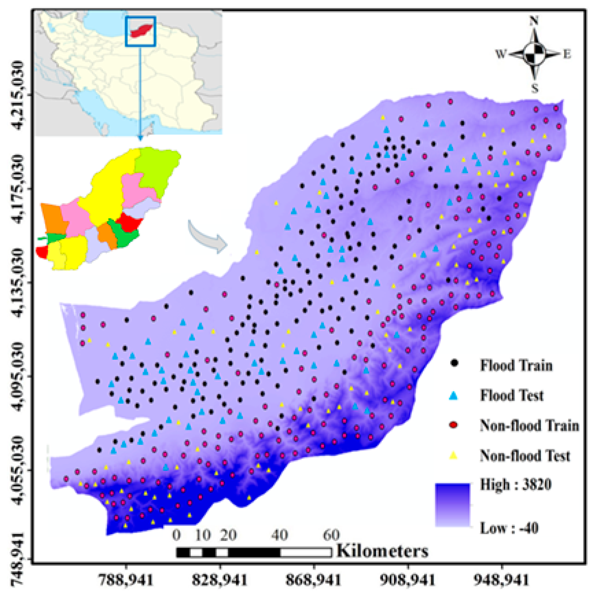
2. Case Study
3. Materials and Methods
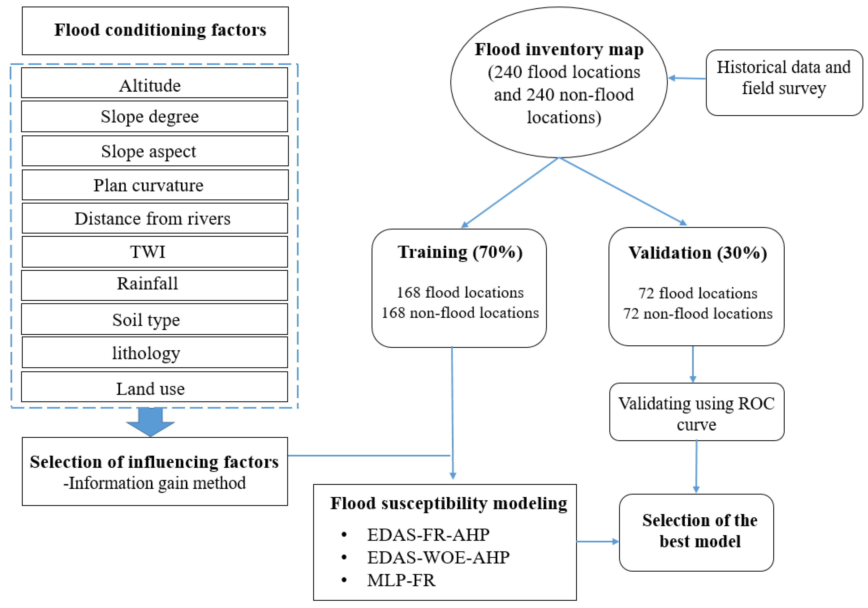
3.1. Research Overview
3.2. Flood Inventory Map
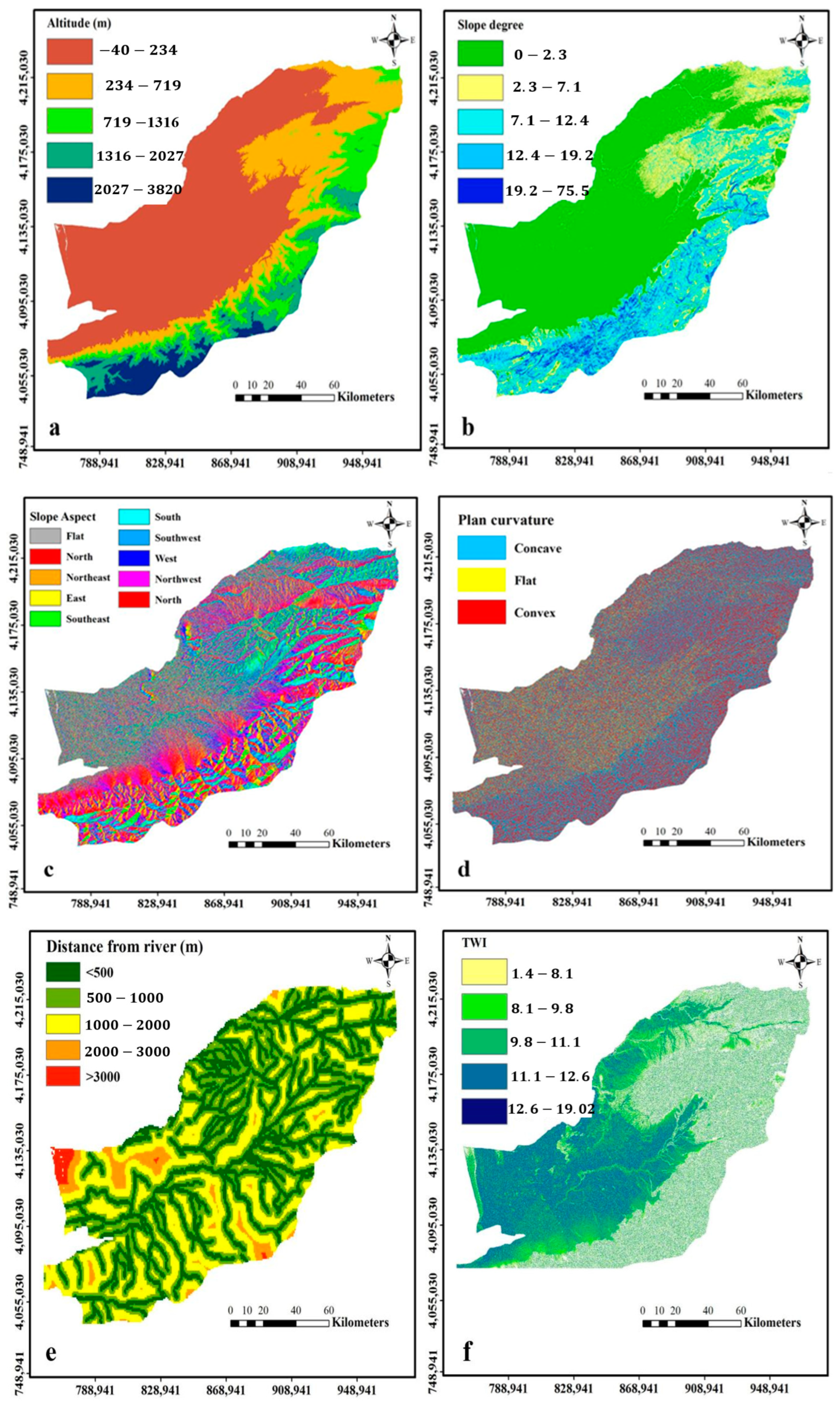
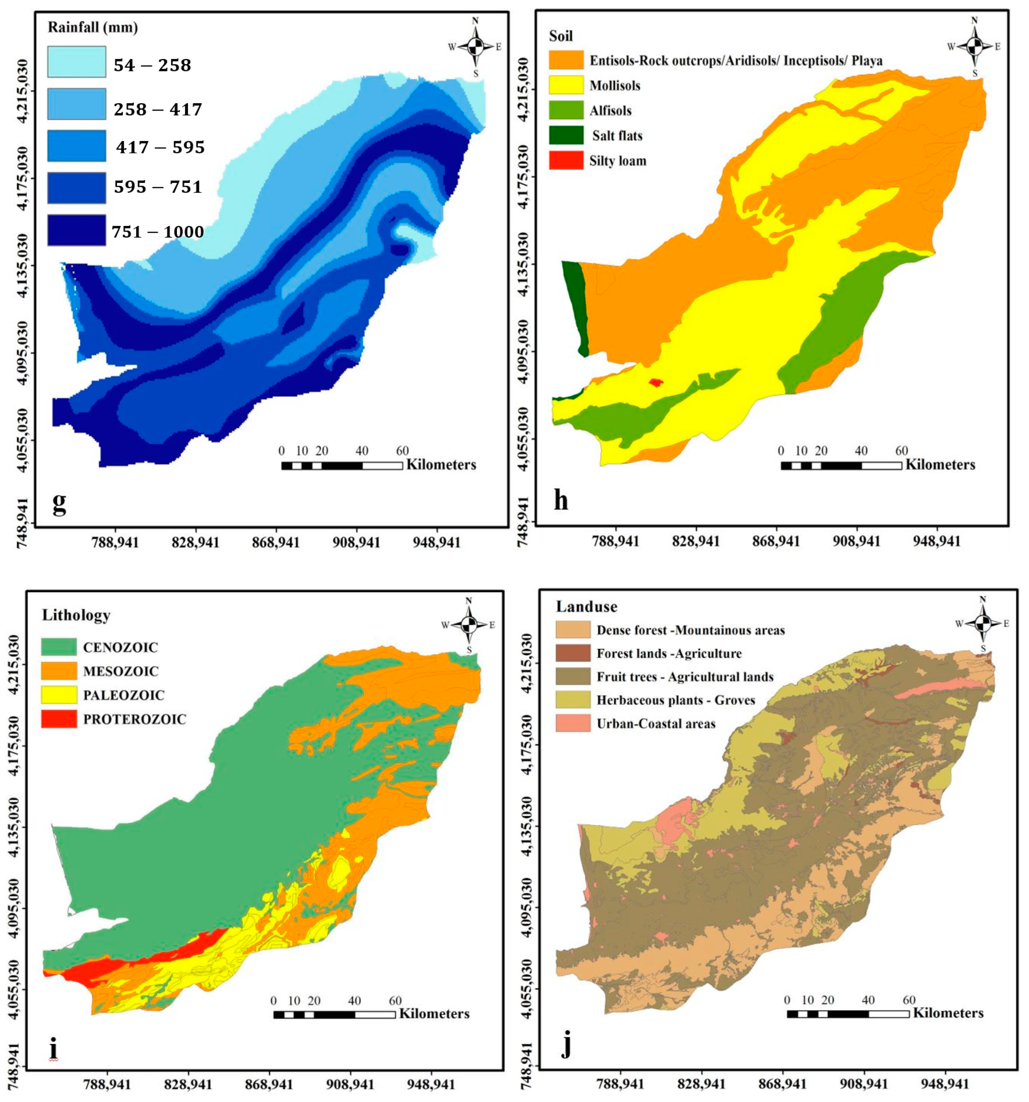
3.3. Flood Influential Criteria
3.4. Feature Selection
3.5. Flood Susceptibility Models
3.5.1. Frequency Ratio
3.5.2. Weights of Evidence
3.5.3. Evaluation Based on Distance from Average Solution
- Step 1. Determining the decision matrix:
- Step 2. Calculation of the average solution of criteria:
- Step 3. Computation of the positive and negative distance from the average value:
- Step 4. Determination of the optimistic () and pessimistic () weighted sum of the positive and negative distances for alternatives:
- Step 5. Normalization of the SP and SN values:
- Step 6. Alternatives ranking:
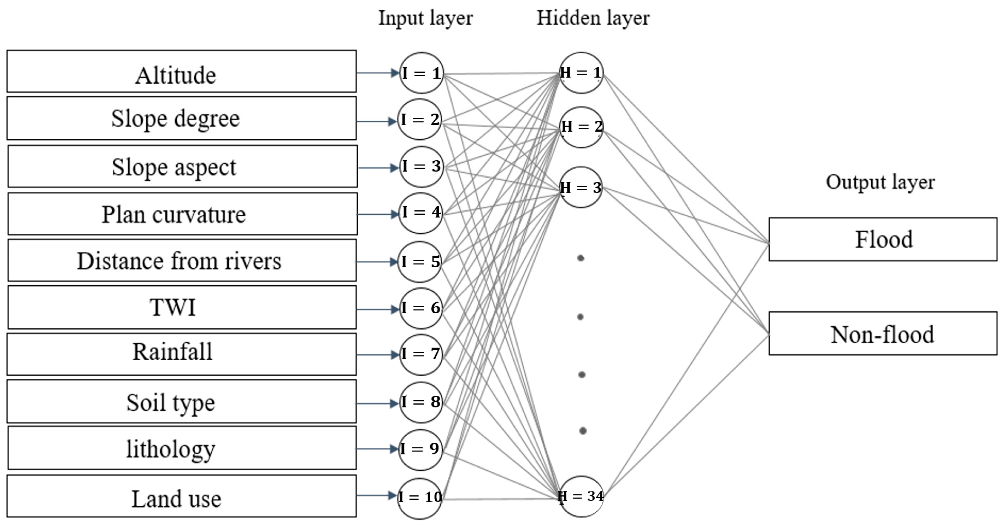
3.5.4. Multilayer Perceptron Layer
- Step 1. Building the architecture of the network:
- Step 2. Training the network:
- Step 3. Testing:
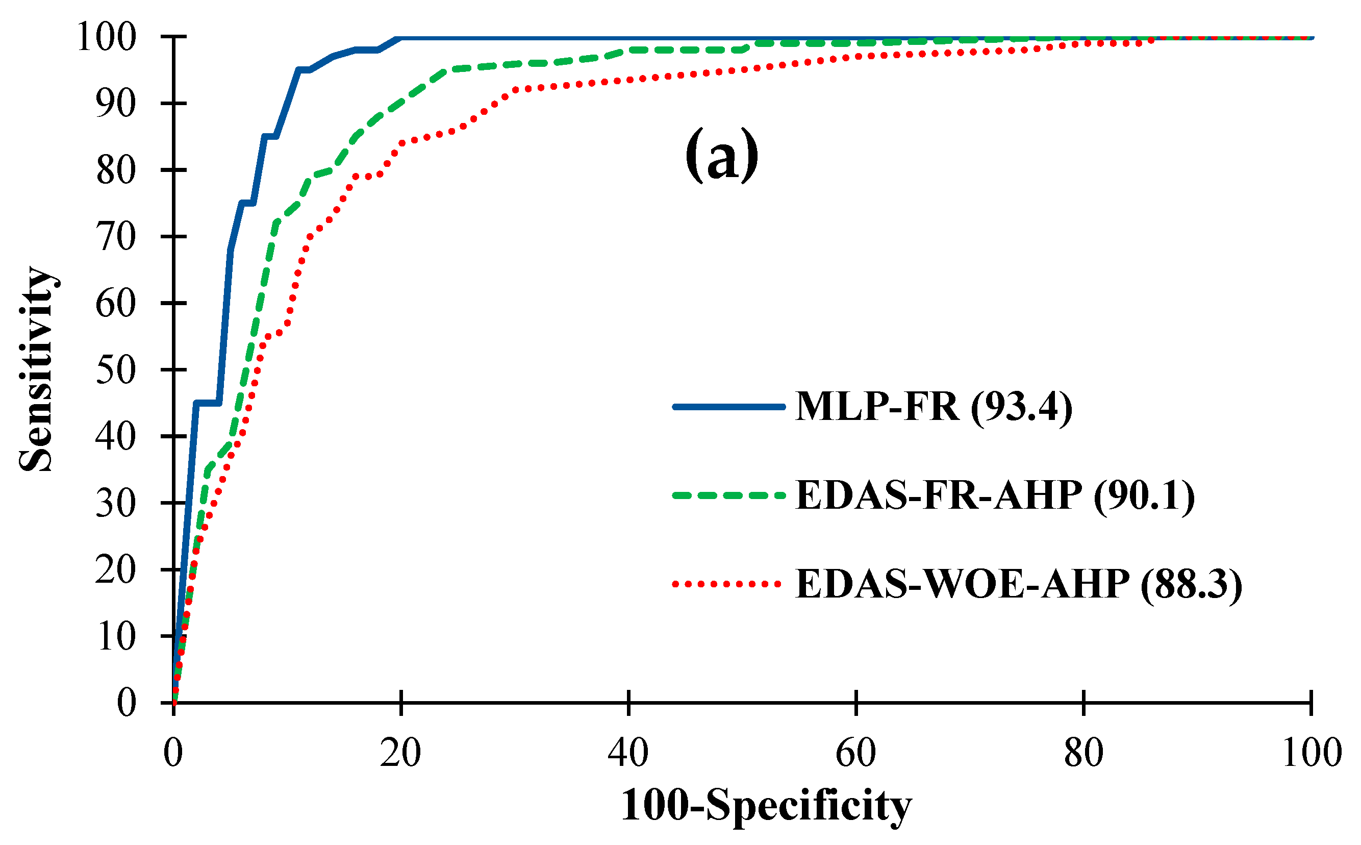
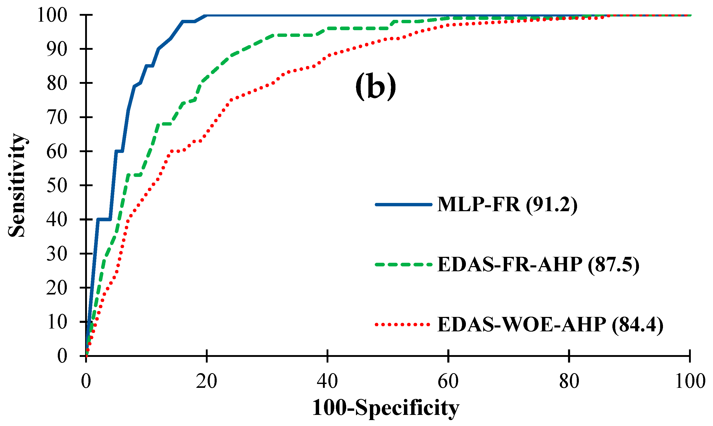
3.6. Validation of Models
4. Results
4.1. Importance of Influential Factors on Flood Occurrence
4.2. Coefficients Calculation
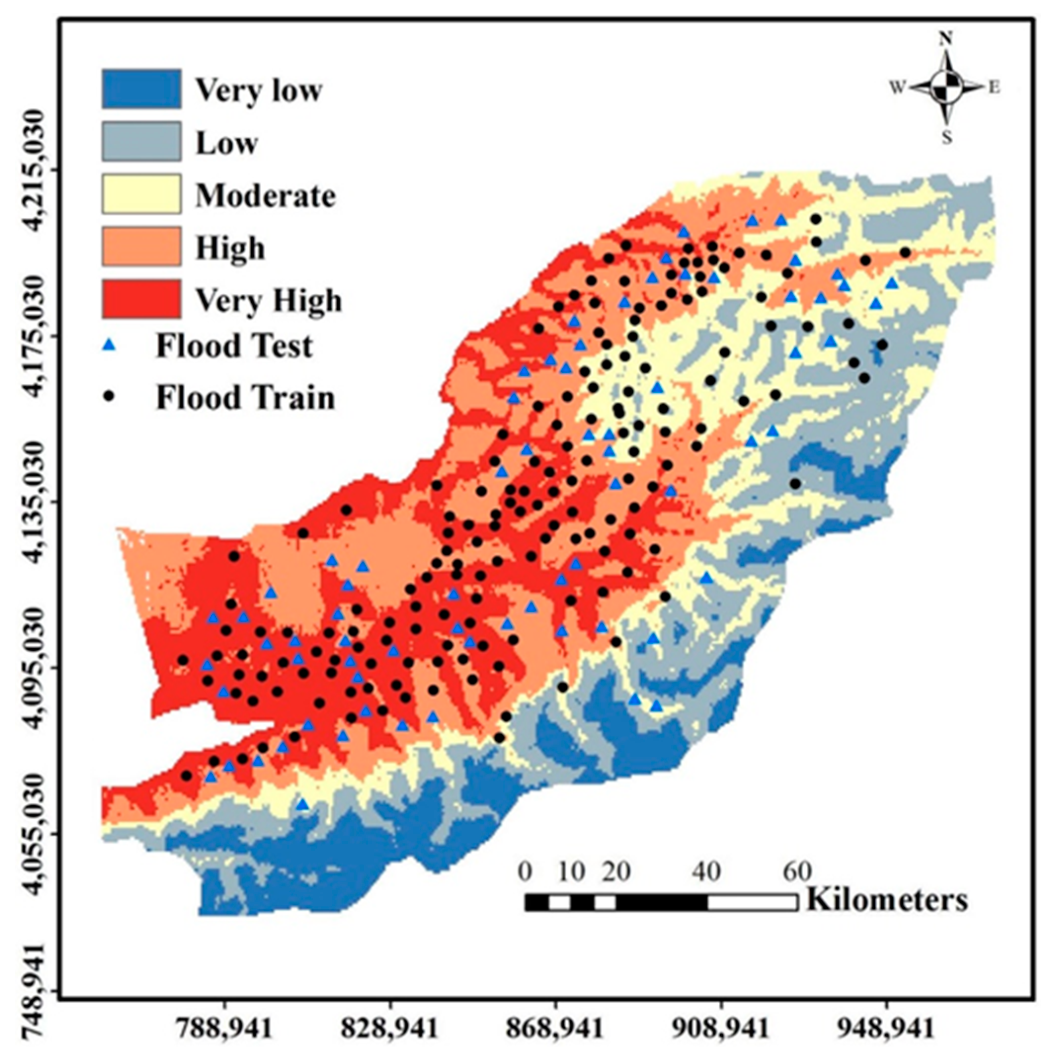
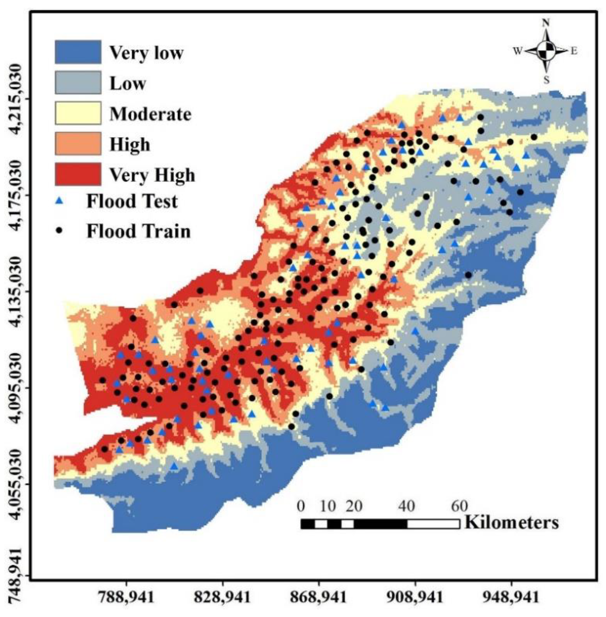
4.3. EDAS-FR-AHP and EDAS-WOE-AHP Methods
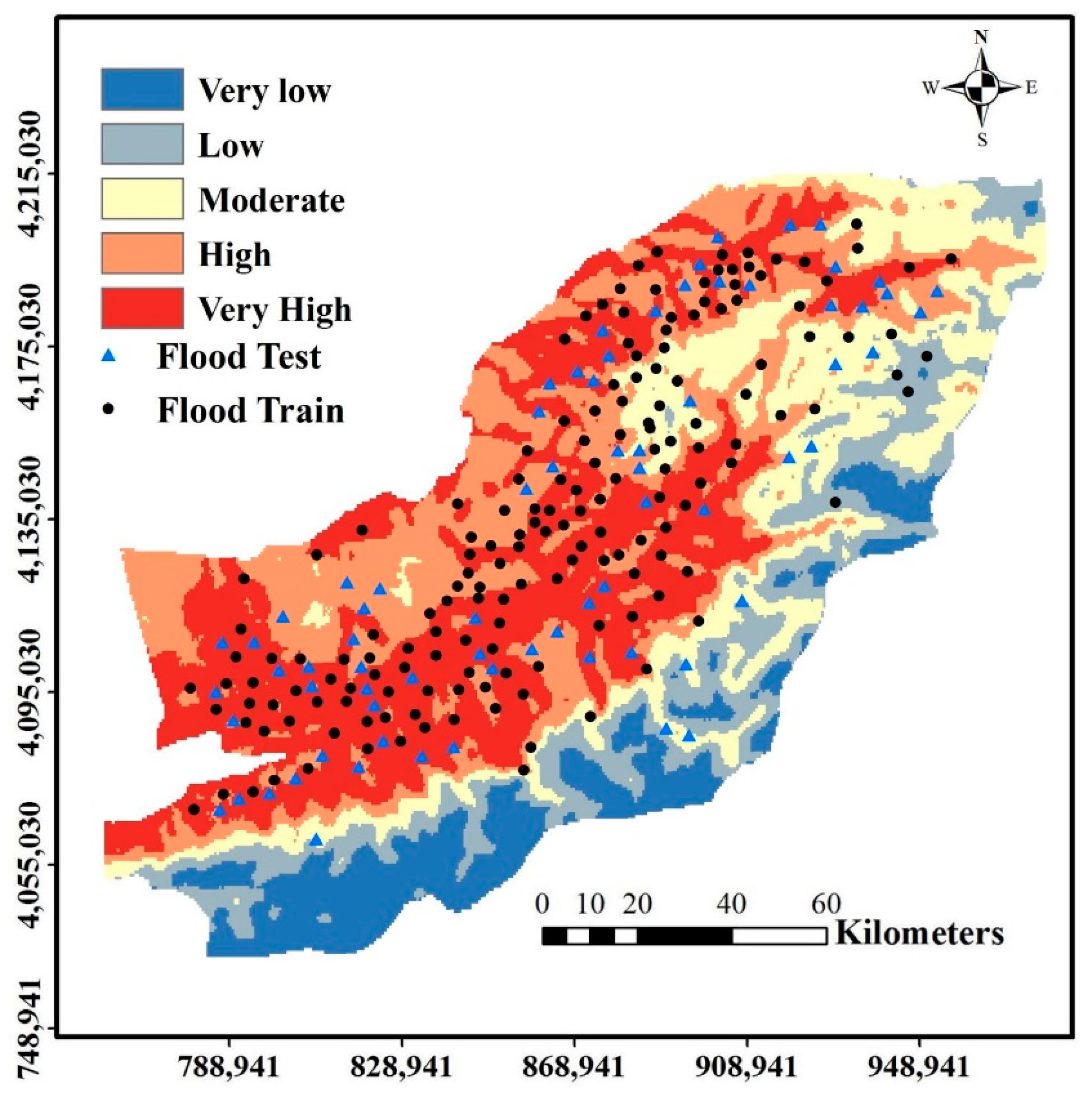
4.4. MLP-FR Method
4.5. Validation
5. Discussions
6. Conclusions
Author Contributions
Funding
Institutional Review Board Statement
Informed Consent Statement
Data Availability Statement
Conflicts of Interest
References
- Shen, G.; Hwang, S.N. Spatial-Temporal snapshots of global natural disaster impacts revealed from EM-DAT for 1900–2015. Geomat. Nat. Hazards Risk 2019, 10, 912–934. [Google Scholar] [CrossRef] [Green Version]
- Pravalie, R.; Bandoc, G.; Patriche, C.; Sternberg, T. Recent changes in global drylands: Evidences from two major aridity databases. CATENA 2019, 178, 209–231. [Google Scholar] [CrossRef]
- Finn, M.P.; Thunen, D. Recent literature in cartography and geographic information science. Cartogr. Geogr. Inf. Sci. 2014, 41, 393–410. [Google Scholar] [CrossRef]
- Foudi, S.; Osés-Eraso, N.; Tamayo, I. Integrated spatial flood risk assessment: The case of Zaragoza. Land Use Policy 2015, 42, 278–292. [Google Scholar] [CrossRef]
- Ouma, Y.O.; Tateishi, R. Urban flood vulnerability and risk mapping using integrated multi-parametric AHP and GIS: Methodological overview and case study assessment. Water 2014, 6, 1515. [Google Scholar] [CrossRef]
- Rahmati, O.; Zeinivand, H.; Besharat, M. Flood hazard zoning in Yasooj region, Iran, using GIS and multi-criteria decision analysis. Geomat. Nat. Hazards Risk 2016, 7, 1000–1017. [Google Scholar] [CrossRef] [Green Version]
- Bubeck, P.; Botzen, W.; Aerts, J. A review of risk perceptions and other factors that influence flood mitigation behavior. Risk Anal. 2012, 32, 1481–1495. [Google Scholar] [CrossRef] [Green Version]
- Omidvar, B.; Khodaei, H. Using value engineering to optimize flood forecasting and flood warning systems: Golestan and Golabdare watersheds in Iran as case studies. Nat. Hazards 2008, 47, 281–296. [Google Scholar] [CrossRef]
- Ahmadlou, M.; Karimi, M.; Alizadeh, S.; Shirzadi, A.; Parvinnejhad, D.; Shahabi, H.; Panahi, M. Flood susceptibility assessment using integration of adaptive network-based fuzzy inference system (ANFIS) and biogeography-based optimization (BBO) and BAT algorithms (BA). Geocarto Int. 2019, 34, 1252–1272. [Google Scholar] [CrossRef]
- Hadian, S.; Tabarestani, E.S.; Pham, Q.B. Multi Attributive Ideal-Real Comparative Analysis (MAIRCA) method for evaluating flood susceptibility in a temperate Mediterranean climate. Hydrol. Sci. J. 2022, 67, 401–418. [Google Scholar] [CrossRef]
- Jaafari, A.; Najafi, A.; Pourghasemi, H.R.; Rezaeian, J.; Sattarian, A. GIS-based frequency ratio and index of entropy models for landslide susceptibility assessment in the Caspian forest, northern Iran. Int. J. Environ. Sci. Technol. 2014, 11, 909–926. [Google Scholar] [CrossRef] [Green Version]
- Lee, M.J.; Kang, J.E.; Jeon, S. Application of frequency ratio model and validation for predictive flooded area susceptibility mapping using GIS. In Proceedings of the 2012 IEEE International Geoscience and Remote Sensing Symposium, Munich, Germany, 22–27 July 2012; pp. 895–898. [Google Scholar] [CrossRef]
- Tehrany, M.S.; Pradhan, B.; Jebur, M.N. Flood susceptibility mapping using a novel ensemble weights-of-evidence and support vector machine models in GIS. J. Hydrol. 2014, 512, 332–343. [Google Scholar] [CrossRef]
- Khosravi, K.; Shahabi, H.; Pham, B.T.; Adamowski, J.; Shirzadi, A.; Pradhan, B.; Hong, H. A comparative assessment of flood susceptibility modeling using Multi-Criteria Decision-Making Analysis and Machine Learning Methods. J. Hydrol. 2016, 573, 311–323. [Google Scholar] [CrossRef]
- Costache, R. Flash-flood Potential Index mapping using weights of evidence, decision Trees models and their novel hybrid integration. Stoch. Environ. Res. Risk Assess. 2019, 33, 1375–1402. [Google Scholar] [CrossRef]
- Luu, C.; Von Meding, J. A flood risk assessment of Quang Nam, Vietnam using spatial multicriteria decision analysis. Water 2018, 10, 461. [Google Scholar] [CrossRef]
- Ogato, G.S.; Bantider, A.; Abebe, K.; Geneletti, D. Geographic information system (GIS)-Based multicriteria analysis of flooding hazard and risk in Ambo Town and its watershed, West shoa zone, oromia regional state, Ethiopia. J. Hydrol. Reg. Stud. 2020, 27, 100659. [Google Scholar] [CrossRef]
- Tabarestani, E.S.; Afzalimehr, H. A comparative assessment of multi-criteria decision analysis for flood susceptibility modelling. Geocarto Int. 2021, 36, 1–24. [Google Scholar] [CrossRef]
- Termeh, S.V.R.; Kornejady, A.; Pourghasemi, H.R.; Keesstra, S. Flood susceptibility mapping using novel ensembles of adaptive neuro fuzzy inference system and metaheuristic algorithms. Sci. Total Environ. 2018, 615, 438–451. [Google Scholar] [CrossRef]
- Jahangir, M.H.; Reineh, S.M.M.; Abolghasemi, M. Spatial predication of flood zonation mapping in Kan River Basin, Iran, using artificial neural network algorithm. Weather. Clim. Extrem. 2019, 25, 100215. [Google Scholar] [CrossRef]
- Zhao, G.; Pang, B.; Xu, Z.; Peng, D.; Zuo, D. Urban flood susceptibility assessment based on convolutional neural networks. J. Hydrol. 2020, 590, 125235. [Google Scholar] [CrossRef]
- Tabarestani, E.S.; Afzalimehr, H. Artificial neural network and multi-criteria decision-making models for flood simulation in GIS: Mazandaran Province, Iran. Stoch. Environ. Res. Risk Assess. 2021, 35, 2439–2457. [Google Scholar] [CrossRef]
- Khosravi, K.; Pham, B.T.; Chapi, K.; Shirzadi, A.; Shahabi, H.; Revhaug, I.; Bui, D.T. A comparative assessment of decision trees algorithms for flash flood susceptibility modeling at Haraz watershed, northern Iran. Sci. Total Environ. 2018, 627, 744–755. [Google Scholar] [CrossRef] [PubMed]
- Pourghasemi, H.R.; Pradhan, B.; Gokceoglu, C. Application of fuzzy logic and analytical hierarchy process (AHP) to landslide susceptibility mapping at Haraz watershed, Iran. Nat. Hazards 2012, 63, 965–996. [Google Scholar] [CrossRef]
- Brito, M.M.; Evers, M. Multi-criteria decision-making for flood risk management: A survey of the current state of the art. Nat. Hazards Earth Syst. Sci. 2016, 16, 1019–1033. [Google Scholar] [CrossRef] [Green Version]
- Ghorabaee, M.K.; Amiri, M.; Zavadskas, E.K.; Turskis, Z.; Antucheviciene, J. Stochastic EDAS method for multi-criteria decision-making with normally distributed data. J. Intell. Fuzzy Syst. 2017, 33, 1627–1638. [Google Scholar] [CrossRef]
- Kia, M.B.; Pirasteh, S.; Pradhan, B.; Mahmud, A.R.; Sulaiman, W.N.A.; Moradi, A. An artificial neural network model for flood simulation using GIS: Johor River Basin, Malaysia. Environ. Earth Sci. 2012, 67, 251–264. [Google Scholar] [CrossRef]
- Lee, S.; Kim, J.C.; Jung, H.S.; Lee, M.J.; Lee, S. Spatial prediction of flood susceptibility using random-forest and boosted-tree models in Seoul metropolitan city, Korea. Geomat. Nat. Hazards Risk 2017, 8, 1185–1203. [Google Scholar] [CrossRef] [Green Version]
- Wang, Y.; Fang, Z.; Hong, H.; Peng, L. Flood susceptibility mapping using convolutional neural network frameworks. J. Hydrol. 2020, 582, 124482. [Google Scholar] [CrossRef]
- Rahmani, S.; Azizian, A.; Samadi, A. New Method for Flood Hazard Mapping in GIS (Case Study: Mazandaran Province Sub-Basins). Iran-Water Resour. Res. 2019, 15, 339–343. [Google Scholar]
- Costache, R.; Barbulescu, A.; Pham, Q.B. Integrated Framework for Detecting the Areas Prone to Flooding Generated by Flash-Floods in Small River Catchments. Water 2021, 13, 758. [Google Scholar] [CrossRef]
- Pham, B.T.; Prakash, I.; Jaafari, A.; Bui, D.T. Spatial Prediction of Rainfall-Induced Landslides Using Aggregating One-Dependence Estimators Classifier. J. Indian Soc. Remote Sens. 2018, 46, 1457–1470. [Google Scholar] [CrossRef]
- Tunusluoglu, M.; Gokceoglu, C.; Nefeslioglu, H.; Sonmez, H. Extraction of potential debris source areas by logistic regression technique: A case study from Barla, Besparmak and Kapi mountains (NW Taurids, Turkey). Environ. Earth Sci. 2008, 54, 9–22. [Google Scholar] [CrossRef]
- Pradhan, B.; Mansor, S.; Pirasteh, S.; Buchroithner, M. Landslide hazard and risk analyses at a landslide prone catchment area using statistical based geospatial model. Int. J. Remote Sens. 2011, 32, 4075–4087. [Google Scholar] [CrossRef]
- Pourtaghi, Z.S.; Pourghasemi, H.R. GIS-based groundwater spring potential assessment and mapping in the Birjand Township, southern Khorasan Province, Iran. Hydrogeol. J. 2014, 22, 643–662. [Google Scholar] [CrossRef]
- Tehrany, S.M.; Shabani, F.; Jebur, M.N.; Hong, H.; Chen, W.; Xie, X. GIS-based spatial prediction of flood prone areas using standalone frequency ratio, logistic regression, weight of evidence and their ensemble techniques. Geomat. Nat. Hazards Risk 2017, 8, 1538–1561. [Google Scholar] [CrossRef]
- Souissi, D.; Zouhri, L.; Hammami, S.; Msaddek, M.H.; Zghibi, A.; Dlala, M. GIS-based MCDM-AHP modeling for flood susceptibility mapping of arid areas, southeastern Tunisia. Geocarto Int. 2019, 35, 991–1017. [Google Scholar] [CrossRef]
- Sidle, R.C.; Ochiai, H. Landslides: Processes, Prediction, and Land Use; Water Res Monograph, 18; American Geophysical Union: Washington, DC, USA, 2006; p. 312. [Google Scholar] [CrossRef]
- Fernandez, D.S.; Lutz, M.A. Urban flood hazard zoning in Tucuman Province, Argentina, using GIS and multicriteria decision analysis. Eng. Geol. 2010, 111, 90–98. [Google Scholar] [CrossRef]
- Moore, I.D.; Grayson, R.B.; Ladson, A.R. Digital terrain modeling: A review of hydrological, geomorphological and biological applications. Hydrol. Process. 1991, 5, 3–30. [Google Scholar] [CrossRef]
- Bui, D.T.; Pradhan, B.; Lofman, O.; Revhaug, I. Landslide susceptibility assessment in Vietnam using support vector machines, decision tree, and naive bayes models. Math. Probl. Eng. 2012, 2012, 1–26. [Google Scholar] [CrossRef] [Green Version]
- Chapi, K.; Singh, V.P.; Shirazi, A.; Shahabi, H.; Bui, D.T.; Pham, B.T.; Khosravi, K. A novel hybrid artificial intelligence approach for flood susceptibility assessment. Environ. Model. Softw. 2017, 95, 229–245. [Google Scholar] [CrossRef]
- Tehrany, M.S.; Pradhan, B.; Jebur, M.N. Spatial prediction of flood susceptible areas using rule based decision tree (DT) and a novel ensemble bivariate and multivariate statistical models in GIS. J. Hydrol. 2013, 504, 69–79. [Google Scholar] [CrossRef]
- Rahmati, O.; Pourghasemi, H.R.; Zeinivand, H. Flood susceptibility mapping using frequency ratio and weights-of-evidence models in the Golestan Province, Iran. Geocarto Int. 2015, 31, 42–70. [Google Scholar] [CrossRef]
- Bonham-Carter, G.F. Geographic Information Systems for Geoscientists: Modeling with GIS. In Computer Methods in the Geosciences; Bonham-Carter, F., Ed.; Pergamon: Oxford, UK, 1994. [Google Scholar]
- Bonham-Carter, G.F.; Agterberg, F.P.; Wright, D.F. Integration of Geological Datasets for Gold Exploration in Nova Scotia; American Society for Photogrammetry and Remote Sensing: Baton Rouge, LA, USA, 1988. [Google Scholar] [CrossRef] [Green Version]
- Youssef, A.M.; Pradhan, B.; Pourghasemi, H.R.; Abdullahi, S. Landslide susceptibility assessment at Wadi Jawrah Basin, Jizan Region, Saudi Arabia using two bivariate models in GIS. Geosci. J. 2015, 19, 449–469. [Google Scholar] [CrossRef]
- Ali, S.A.; Parvin, F.; Pham, Q.B.; Vojtek, M.; Vojteková, J.; Costache, R.; Linh, N.T.T.; Nguyen, H.Q.; Ahmad, A.; Ghorbani, M.A. GIS-Based Comparative Assessment of Flood Susceptibility Mapping Using Hybrid Multi-Criteria Decision-Making Approach, Naïve Bayes Tree, Bivariate Statistics and Logistic Regression: A Case of Top’a Basin, Slovakia. Ecol. Indic. 2020, 117, 106620. [Google Scholar] [CrossRef]
- Saaty, T.L. A scaling method for priorities in hierarchical structures. J. Math. Psychol. 1977, 15, 234–281. [Google Scholar] [CrossRef]
- Yang, X.; Ding, J.; Hou, H. Application of a triangular fuzzy AHP approach for flood risk evaluation and response measures analysis. Nat. Hazards 2013, 68, 657–674. [Google Scholar] [CrossRef]
- Suthirat, K.; Athit, P.; Patchapun, R.; Brundiers, K.; Buizer, J.L.; Melnick, R. AHP-GIS analysis for flood hazard assessment of the communities nearby the world heritage site on Ayutthaya Island, Thailand. Int. J. Disaster Risk Reduct. 2020, 48, 101612. [Google Scholar] [CrossRef]
- Zare, M.; Pourghasemi, H.R.; Vafakhah, M.; Pradhan, B. Landslide susceptibility mapping at Vaz Watershed (Iran) using an artificial neural network model: A comparison between multilayer perceptron (MLP) and radial basic function (RBF) algorithms. Arab. J. Geosci. 2013, 6, 2873–2888. [Google Scholar] [CrossRef]
- Costache, R.; Pham, Q.B.; Sharifi, E.; Linh, N.T.T.; Abba, S.I.; Vojtek, M.; Vojteková, J.; Nhi, P.T.T.; Khoi, D.N. Flash-Flood Susceptibility Assessment Using Multi-Criteria Decision Making and Machine Learning Supported by Remote Sensing and GIS Techniques. Remote Sens. 2020, 12, 106. [Google Scholar] [CrossRef] [Green Version]
- Rahmati, O.; Samani, A.N.; Mahdavi, M.; Pourghasemi, H.R.; Zeinivand, H. Groundwater potential mapping at Kurdistan region of Iran using analytic hierarchy process and GIS. Arab. J. Geosci. 2014, 8, 7059–7071. [Google Scholar] [CrossRef]
- Shirzadi, A.; Bui, D.T.; Pham, B.T.; Solaimani, K.; Chapi, K. Shallow landslide susceptibility assessment using a novel hybrid intelligence approach. Environ. Earth Sci. 2017, 76, 60. [Google Scholar] [CrossRef]
- Chen, W.; Zhang, S.; Li, R.; Shahabi, H. Performance evaluation of the GIS-based data mining techniques of best-first decision tree, random forest, and naïve Bayes tree for landslide susceptibility modeling. Sci. Total Environ. 2018, 644, 1006–1018. [Google Scholar] [CrossRef] [PubMed]
- Jung, I.W.; Chang, H.; Moradkhani, H. Quantifying uncertainty in urban flooding analysis considering hydro-climatic projection and urban development effects. Hydrol. Earth Syst. Sci. 2011, 15, 617–633. [Google Scholar] [CrossRef] [Green Version]
- Osaragi, T. Classification Methods for Spatial Data Representation; Centre for Advanced Spatial Analysis: London, UK, 2002. [Google Scholar]
- Rahman, M.; Ningsheng, C.; Islam, M.M.; Dewan, A.; Iqbal, J.; Washakh, R.M.A.; Shufeng, T. Flood Susceptibility Assessment in Bangladesh Using Machine Learning and Multi-criteria Decision Analysis. Earth Syst. Environ. 2019, 3, 123. [Google Scholar] [CrossRef]
- Kotsiantis, S.B.; Zaharakis, I.; Pintelas, P. Supervised machine learning: A review of classification techniques. Emerg. Artif. Intell. Appl. Comput. Eng. 2007, 160, 3–24. [Google Scholar] [CrossRef]
- Ahmadlou, M.; A’kif, A.; Rahman, A.A.; Aman, A.; Rida, A.; Quoc, B.P.; Nadhir, A.; Nguyen, T.T.L.; Hedieh, S. Flood susceptibility mapping and assessment using a novel deep learning model combining multilayer perceptron and autoencoder neural networks. J. Flood Risk Manag. 2021, 14, e12683. [Google Scholar] [CrossRef]


| Dataset | Source | Data Type | The Scale of Source Data | Derived Factors |
|---|---|---|---|---|
| Digital elevation model (DEM) | United States Geological Survey (USGS) site | Raster | 1:25,000 | Altitude, slope, aspect, curvature, distance from rivers, TWI |
| Rainfall | Golestan meteorology organization | Vector | 1:25,000 | Rainfall map |
| Geological map | Golestan Regional Water Authority | Vector | 1:100,000 | Lithology, soil type |
| Land cover | Golestan Regional Water Authority | Vector | 1:100,000 | Land use |
| Flood Influential Factor | IG | Flood Influential Factor | IG |
|---|---|---|---|
| Altitude | 0.69 | TWI | 0.42 |
| Slope | 0.78 | Rainfall | 0.35 |
| Aspect | 0.12 | Soil type | 0.23 |
| Plan curvature | 0.47 | Lithology | 0.51 |
| Distance from rivers | 0.73 | Land use | 0.57 |
| Criteria | Class | Number of Pixel | Number of Floods | C/Sc | FR | AHP | AHP × FR | AHP × C/Sc |
|---|---|---|---|---|---|---|---|---|
| Altitude | 2027–3820 | 144,558 | 1 | −2.147 | 0.121 | 0.32 | 0.039 | −0.687 |
| 1316–2027 | 233,726 | 1 | −2.658 | 0.075 | 0.024 | −0.851 | ||
| 719–1316 | 365,764 | 12 | −2.039 | 0.576 | 0.184 | −0.652 | ||
| 234–719 | 589,554 | 25 | −1.651 | 0.744 | 0.238 | −0.528 | ||
| −40–234 | 1,613,803 | 129 | 5.503 | 1.402 | 0.449 | 1.761 | ||
| Slope | 19.2–75.5 | 80,633 | 4 | −0.282 | 0.870 | 0.09 | 0.078 | −0.025 |
| 12.4–19.2 | 229,861 | 10 | −0.889 | 0.763 | 0.069 | −0.080 | ||
| 7.1–12.4 | 400,470 | 22 | −0.186 | 0.964 | 0.087 | −0.017 | ||
| 2.3–7.1 | 589,786 | 32 | −0.312 | 0.952 | 0.086 | −0.028 | ||
| 0–2.3 | 1,646,655 | 101 | 1.108 | 1.076 | 0.097 | 0.100 | ||
| Aspect | Flat | 12,050 | 6 | 5.290 | 8.736 | 0.02 | 0.175 | 0.106 |
| North | 437,462 | 23 | −0.420 | 0.922 | 0.018 | −0.008 | ||
| Northeast | 338,379 | 18 | −0.311 | 0.933 | 0.019 | −0.006 | ||
| East | 316,204 | 20 | 0.492 | 1.110 | 0.022 | 0.010 | ||
| Souteast | 366,613 | 16 | −1.140 | 0.766 | 0.015 | −0.023 | ||
| South | 434,844 | 20 | −1.038 | 0.807 | 0.016 | −0.021 | ||
| Southwest | 337,394 | 22 | 0.670 | 1.144 | 0.023 | 0.013 | ||
| West | 323,159 | 21 | 0.637 | 1.140 | 0.023 | 0.013 | ||
| Northwest | 381,300 | 22 | 0.061 | 1.012 | 0.020 | 0.001 | ||
| Plan Curvature | Concave | 1,393,068 | 66 | −2.062 | 0.831 | 0.1 | 0.083 | −0.206 |
| Convex | 1,360,360 | 76 | −0.238 | 0.980 | 0.098 | −0.024 | ||
| Flat | 193,977 | 26 | 4.477 | 2.352 | 0.235 | 0.448 | ||
| Distance from river | >3000 | 53,994 | 2 | −0.615 | 0.650 | 0.17 | 0.110 | −0.105 |
| 2000–3000 | 342,862 | 10 | −2.246 | 0.512 | 0.087 | −0.382 | ||
| 1000–2000 | 1,045,667 | 22 | −5.660 | 0.369 | 0.063 | −0.962 | ||
| 500–1000 | 1,131,426 | 71 | 1.032 | 1.101 | 0.187 | 0.175 | ||
| <500 | 373,457 | 63 | 8.907 | 2.960 | 0.503 | 1.514 | ||
| TWI | 1.4–8.1 | 133,167 | 3 | −1.642 | 0.395 | 0.05 | 0.020 | −0.082 |
| 8.1–9.8 | 544,028 | 17 | −2.730 | 0.548 | 0.027 | −0.137 | ||
| 9.8–11.1 | 1,016,028 | 49 | −1.443 | 0.846 | 0.042 | −0.072 | ||
| 11.1–12.6 | 875,180 | 55 | 0.863 | 1.103 | 0.055 | 0.043 | ||
| 12.6–19.02 | 379,002 | 44 | 5.000 | 2.037 | 0.102 | 0.250 | ||
| Rainfall | 54–258 | 309,529 | 14 | −0.914 | 0.794 | 0.07 | 0.056 | −0.064 |
| 258–417 | 689,864 | 46 | 1.215 | 1.170 | 0.082 | 0.085 | ||
| 417–595 | 446,783 | 12 | −2.813 | 0.471 | 0.033 | −0.197 | ||
| 595–751 | 864,585 | 24 | −4.139 | 0.487 | 0.034 | −0.290 | ||
| 751–1000 | 636,644 | 72 | 6.423 | 1.984 | 0.139 | 0.450 | ||
| Soil type | Entisols-Rock Outcrops/Aridisols/Inceptisols/Playa | 1,345,296 | 76 | −0.105 | 0.991 | 0.05 | 0.050 | −0.005 |
| Mollisols | 1,225,408 | 88 | 2.819 | 1.260 | 0.063 | 0.141 | ||
| Alfisols | 327,844 | 2 | −3.290 | 0.107 | 0.005 | −0.165 | ||
| Salt flats | 46,135 | 1 | −0.974 | 0.380 | 0.019 | −0.049 | ||
| Silty loam | 2723 | 1 | 1.862 | 6.443 | 0.322 | 0.093 | ||
| Litologhy | Paleozoic | 226,1742 | 2 | −7.890 | 0.016 | 0.04 | 0.001 | −0.316 |
| Mesozoic | 331,254 | 10 | −2.127 | 0.530 | 0.021 | −0.085 | ||
| Proterozoic | 1166 | 1 | 2.708 | 15.052 | 0.602 | 0.108 | ||
| Cenozoic | 353,244 | 155 | 15.488 | 7.698 | 0.308 | 0.620 | ||
| Land use | Dense forest—Mountainous areas | 702,647 | 7 | −5.113 | 0.175 | 0.07 | 0.012 | −0.358 |
| Forest lands—Agriculture | 28,730 | 3 | 1.053 | 1.832 | 0.128 | 0.074 | ||
| Fruit trees—Agricultural lands | 1,610,365 | 118 | 3.986 | 1.286 | 0.090 | 0.279 | ||
| Herbaceous plants—Groves | 487,559 | 21 | −1.404 | 0.756 | 0.053 | −0.098 | ||
| Urban–Coastal areas | 118,104 | 19 | 4.584 | 2.822 | 0.198 | 0.321 |
| Training | Testing | |
|---|---|---|
| Sensitivity | 0.864 | 0.851 |
| Specificity | 0.912 | 0.893 |
| Accuracy | 0.892 | 0.876 |
Publisher’s Note: MDPI stays neutral with regard to jurisdictional claims in published maps and institutional affiliations. |
© 2022 by the authors. Licensee MDPI, Basel, Switzerland. This article is an open access article distributed under the terms and conditions of the Creative Commons Attribution (CC BY) license (https://creativecommons.org/licenses/by/4.0/).
Share and Cite
Hadian, S.; Afzalimehr, H.; Soltani, N.; Tabarestani, E.S.; Karakouzian, M.; Nazari-Sharabian, M. Determining Flood Zonation Maps, Using New Ensembles of Multi-Criteria Decision-Making, Bivariate Statistics, and Artificial Neural Network. Water 2022, 14, 1721. https://doi.org/10.3390/w14111721
Hadian S, Afzalimehr H, Soltani N, Tabarestani ES, Karakouzian M, Nazari-Sharabian M. Determining Flood Zonation Maps, Using New Ensembles of Multi-Criteria Decision-Making, Bivariate Statistics, and Artificial Neural Network. Water. 2022; 14(11):1721. https://doi.org/10.3390/w14111721
Chicago/Turabian StyleHadian, Sanaz, Hossein Afzalimehr, Negar Soltani, Ehsan Shahiri Tabarestani, Moses Karakouzian, and Mohammad Nazari-Sharabian. 2022. "Determining Flood Zonation Maps, Using New Ensembles of Multi-Criteria Decision-Making, Bivariate Statistics, and Artificial Neural Network" Water 14, no. 11: 1721. https://doi.org/10.3390/w14111721