Sea Level Variation and Trend Analysis by Comparing Mann–Kendall Test and Innovative Trend Analysis in Front of the Red River Delta, Vietnam (1961–2020)

Abstract

In this study, we analyze sea surface height referenced against the WGS84 ellipsoid at the Hon Dau tidal gauge station (Hai Phong, Vietnam), in front of the Red River Delta, between 1961 and 2020. The annual sea level varied from 165.23 cm to 206.06 cm in this period (+20.28 cm over 60 years). The average water level was 190.87 cm for 60 years, with higher annual values in recent years, especially from 2016 to the present (above 201.5 cm). The Mann–Kendall (MK) test with Sen’s slope estimator and Şen’s innovative trend analysis (ITA) were applied and compared to estimate the sea level rise. These methods showed complete agreement among tests with significant rising trends of about 3.38 mm/year with the MK test and 3.08 mm/year with the ITA method for 1961–2020. During the last 20 years (2001–2020), the mean sea level increased about 7.16 mm/year (MK test and Sen’s slope), 7.38 mm/year (ITA method), and around twice higher than the rate of the region and globally. The MK test and ITA method provided similar results for periods: 1961–2020, 1961–1980, and 2001–2020, with relatively stable monotonic related trend conditions. For the period 1981–2000, with a more nonmonotonic trend, the MK test and ITA method provided different trends and allowed to illustrate the specificity of each method.

1. Introduction

Sea level rise (SLR) is one of the most significant effects of climate change, which causes severe impacts in various parts of the world. The IPCC (2021) reported that the global average rate of SLR has increased faster than expected in a few recent decades: 1.3 mm/year (1901–1971), 1.9 mm/year (1971–2006), and 3.7 mm/year (2006–2018) [1].

Unlike infrequent large typhoons or earthquakes that can reshape the coastline within hours, the impacts of SLR are typically slow, repetitive, and cumulative [2]. Immediate effects include submergence, increased flooding, and saltwater intrusion into surface water, whereas long-term effects will increase coastal erosion and cause saltwater intrusion into groundwater. In addition, coastal wetlands will struggle to keep pace with SLR if sediment supplies are insufficient [3]. The effects of SLR have significant consequences for many coastal communities worldwide [4] with strong socioeconomic impacts. Increased coastal erosion due to accelerated SLR poses a severe threat to economies worldwide. As the population increases, coastal areas are also likely to experience additional stresses from land use and hydrological changes [5]. These changes can have devastating effects on coastal habitats further inland, leading to flooding of wetlands, salt contamination of aquifers and agricultural soils, and loss of habitat for fish, birds, plants, and many species [6,7,8].

The water elevation of the sea varies in time and space due to physical processes, such as tide and waves. Mean sea level at a given position is defined as the height of the sea surface averaged over a period, such as a month or a year, long enough to essentially eliminate fluctuations caused by tide and waves [9]. It also has a spatial distribution on a global scale due to phenomena that dominate regional and local scales. As a result, local mean sea level changes usually differ from global oceans. In the South China Sea, the sea level has continued to rise [10,11]. Li et al. [12] reported that the mean sea level in the South China Sea rose by about 1.0 cm/year from 1993 to 1999.

Climatologic and hydrological trend analyses have several approaches, such as the Mann–Kendall (MK) trend test and the Sen slope estimator [13]. One of the commonly used nonparametric trend tests is the MK test. The MK test and Sen’s slope are determined by the ranks and sequences of time series rather than the original values. They are robust when dealing with non-normally distributed data, censored data, and time series with missing values [14], which are commonly encountered in hydrometeorological time series [15,16,17]. This method is widely used in many types of research due to some advantages: it is not affected by missing data and by the length of time series; it can tolerate outliers in data and is less affected than other methods to outliers [18,19] and only require data to be independent [20,21,22,23]. Combined with the Sen’s slope, the MK test has been widely utilized for detecting trends in hydrometeorological time series, such as groundwater [24], water quality [25,26], streamflow [27,28], lake level [29], temperature and precipitation [30,31], and SLR [32,33,34,35].

The major disadvantage of the method is the influence of autocorrelation in data on its significance test. Several modifications in the MK test have been proposed to avoid the effect of autocorrelation through the prewhitening of data [36,37]. However, recent research has proved that those are not sufficient to exclude the impact of long-term dependency on the data series on MK trend significance [38]. Some local factors (e.g., topography, water river discharges, earth–atmosphere fluxes) often cause a localized change in water temperature, which makes the trend noisy. Therefore, it is necessary to have a flexible graphical technique to explore data trends to avoid significant hidden trends [39]. Among them, the innovative trend analysis (ITA) method, recommended by Şen [40], has been applied to discover the trend in rainfall, streamflow, pan evaporation, and water quality parameters in different regions of the world [39,41,42,43]. Several advantages of the ITA method were shown when compared with other methods in these studies. Ay and Kisi [44] analyzed the trends of monthly total rainfall in the Black Sea and Central Anatolia regions based on MK and the ITA methods. According to Kisi [22], hidden trends in pan evaporation are mainly identified by the graphical plots of the ITA method than the MK tests. Those studies show that the ITA method allows robust trend estimation by ignoring the seasonal cycle and time series length. It examines any hidden subtrends present in the series. Thus, the ITA method can estimate a monotonic trend current in the time series that persist with time.

Vietnam is considered one of the countries most affected by climate change [45,46,47]. Thus, many studies have estimated the manifestations of climate change here, especially SLR. According to Tuong [48], SLR varied between 1.75 and 2.56 mm/year during 1961–2000 in four coastal stations of Vietnam: Hon Dau (North), Da Nang, Quy Nhon (Center), and Vung Tau (South). MONRE [49] reported that the mean sea level of all tide gauges was 2.45 mm/year and increased significantly in 1993–2014, with 3.34 mm/year. Ca [34] illustrated that sea level at the Hon Dau tide gauge increased by 2.5 mm/year from 1957 to 2012. Recently, Hai et al. [50] applied the MK test and calculated the trend of SLR by the Sen’s slope at Hon Dau tide gauge, in the Hai Phong coastal area, from 1960 to 2020. However, the results of MK test did not provide a visual–graphical illustration of trends and may not show an entirely hidden trend (e.g., nonmonotonic trends). Therefore, this study is to identify sea level variation and trend magnitude of monthly and annual sea level at the Hon Dau tidal gauge station by comparing the MK test with Sen’s slope and the ITA method for the period 1961–2020 and subperiods: 1961–1980, 1981–2000, and 2001–2020. The results of this study give new knowledge about sea level variation in the Gulf of Tonkin, North Vietnam, and they help to improve its trend identification.

2. Material and Methods

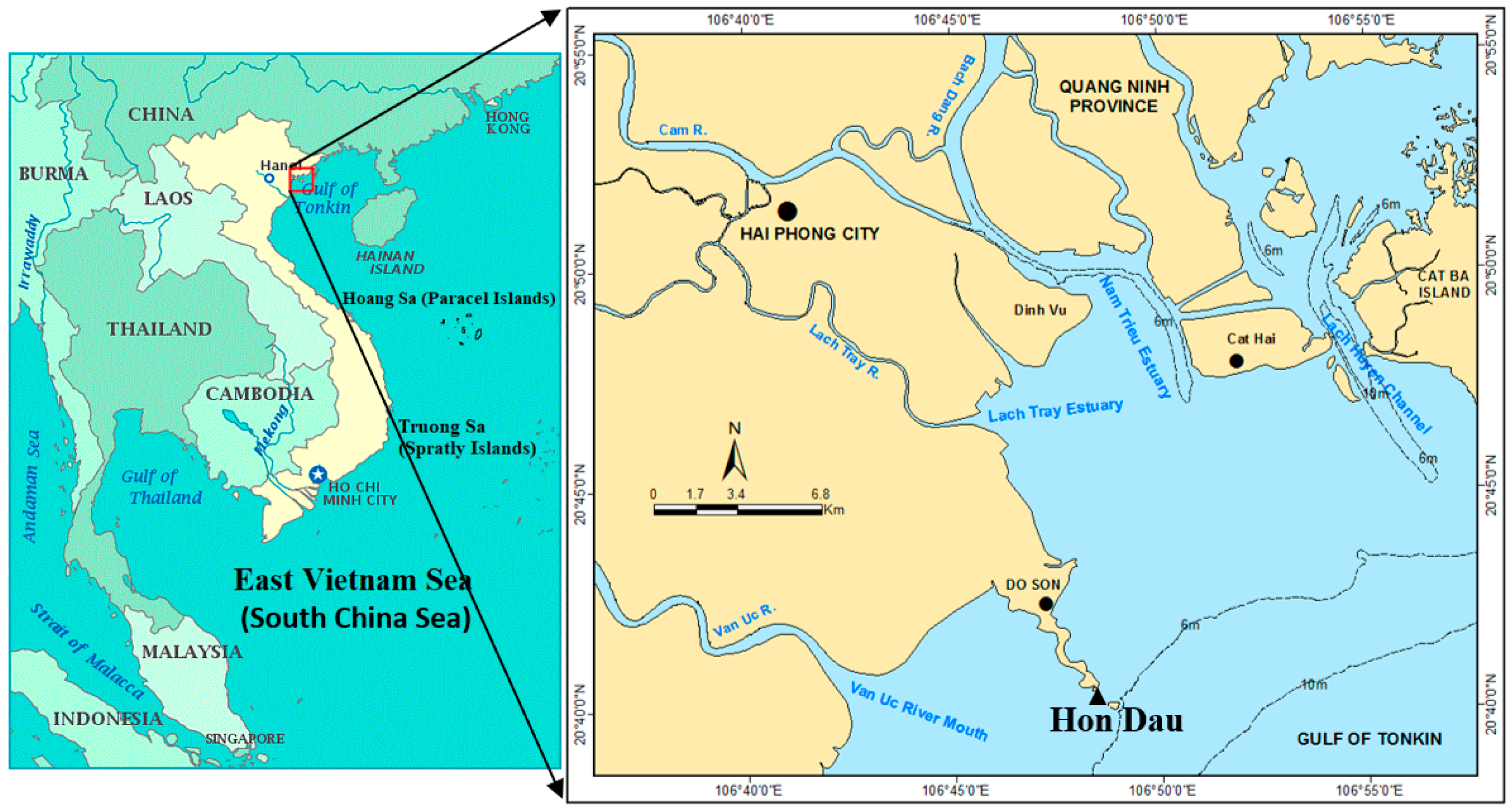
2.1. Hai Phong Coastal Area

The Hai Phong coastal area is situated in the western part of the Tonkin Gulf, with high biodiversity, affluent marine resources, and high economic activities. Hai Phong is the third-largest city in Vietnam and has the largest seaport in the northern region [51]. Based on observations for 60 years (1958–2017) at the Hon Dau station, the average air temperature was 23.8 °C. While the average temperature was below 20 °C in winter, it was above 27 °C in summer. Analysis of measurements over 1958–2017 at the Hon Dau station showed that the average annual rainfall was 1563 mm. The rainy season was extended from May to October, with an average rainfall of 350 mm [52].

This area is strongly impacted by its hydrological regime. River flow encompasses substantial seasonal variations, with 71–79% of the total annual water discharge in the rainy season and only 9.4–18% during the dry season [53]. In addition, it is influenced by diurnal tide, with an amplitude of 2.6–3.6 m in spring tide and about 0.5–1.0 m in the neap tide. Some recent studies have also shown that the coastal area of Hai Phong is affected by climate change. Sea surface warming trend was +0.02 °C/year for the period 1995–2020 and of +0.093 °C/year for the period 2008–2020 [54]; the average annual rise of sea level was 7.78 mm/year over the periods 2002–2020 [50].

2.2. Data

Hourly sea level measurements at the Hon Dau station (20°40′ N–106°49′ E) (Figure 1) were collected by the Vietnam Hydro-Meteorological Data and Information Center and analyzed from 1961 to 2020 (60 years) to calculate the sea level trend. Before 2015, a tidal recorder CYM type (made in Russia) was used to measure water elevation at Hon Dau. Since 2015, the tidal data at Hon Dau have been measured by a Stevens Type A-04 gauge (made in USA). These data are the sea surface height above a reference level—chart datum (+1.86 m below mean sea level), with its reference ellipsoid as WGS.84 ellipsoid, its origin at the Hanoi permanent GPS station and UTM projection.

The Hon Dau station locates next to Hon Dau Island (Figure 1), about 15–20 km south of Hai Phong city. Therefore, sea level data at Hon Dau can represent the coastal area with a radius of 15–20 km of Hai Phong coastal area. This study also analyzed variation and trends of sea level data in three successive 20-year subperiods from 1961 to 2020 to clarify the changes in trends.

This study also used the delayed-time gridded (a resolution at 0.25° × 0.25°) monthly mean of sea level anomalies (SLA), estimated from multisatellite altimeter data from 1993 to 2020 from Archiving, Validation and Interpretation of the Satellite Oceanographic data (AVISO) in France. They are calculated by averaging the sea level anomalies over a same month for all the years. The monthly mean of SLA is estimated by the sea surface height (SSH) above the reference ellipsoid and the mean sea surface (MSS) over a period (https://www.aviso.altimetry.fr/en/data.html, accessed on 10 October 2021).

Furthermore, monthly mean Oceanic Niño Index (ONI) data for the period 1961–2020 were extracted from the NOAA Center for Weather and Climate Prediction database (http://www.cpc.ncep.noaa.gov, accessed on 10 October 2021). Being based on the three-month moving average of the SST anomaly in the Niño 3.4 region (5° N–5° S, 120° W–170° W), the ONI is used to identify El Niño (warm) and La Niña (cold) events in the Tropical Pacific. An El Niño event is considered when the ONI exceeds the threshold value +0.5 °C for at least five consecutive months. Conversely, La Niña events are defined as periods with at least five consecutive months with an ONI below −0.5 °C [55].

2.3. Methods

2.3.1. Sea Level Anomaly from Tidal Gauge Station

Monthly mean SLA from the AVISO is gridded product with a spatial resolution of 0.25° × 0.25°. Therefore, to compare between satellite-altimetry-derived SLAs and tide gauge observed SLAs, we extracted data from a position at the closest point to the Hon Dau station from 1993–2020. This point is coordinated at 20°37.5′ N-106°52.5′ E. Monthly mean SLA_i at the Hon Dau station during 1993–2020 was defined as:

SLA_i = SSH_i − SSH_1993–2020

(1)

where SSH_i is the monthly mean sea surface heigh, and SSH_1993–2020 is the mean sea surface height at Hon Dau during 1993–2020.

2.3.2. The Mann–Kendall Test

The Mann–Kendall test is a widely used statistical test for analyzing the trend in climatological and hydrological time series. It avoids the local maximum values of the data series. The null hypothesis, H₀, is that the data come from a population with independent realizations that do not follow any trend. The alternative hypothesis, H₁, is that the data follow a clear trend.

The Mann–Kendall S statistic is determined by analyzing all possible pairs of measurements in the data set. If the later value is greater in magnitude than an earlier one, S is incremented by one. On the other hand, if a later value is less in magnitude than an earlier sample, S is decremented by one.

The Mann–Kendall statistic parameter, S, is computed as follows:

$$S={\displaystyle \sum }_{i=1}^{n-1}{\displaystyle \sum }_{j=i+1}^{n}sign\left(X_j-X_i\right)$$

(2)

where X_i and X_j are random variables (divided the given time series X into two variable sets, as X₁, X₂, …, X_i, and X_{i + 1}, X_{i + 2},…, X_j).

$$Sign \left(X_j-X_i\right)=\{ \begin{array}{c}1 if X_j-X_i>0\\ 0 if X_j-X_i=0\\ -1 if X_j-X_i<0\end{array}$$

(3)

The variance of S, VAR(S), is given by

$$VAR\left(S\right)=\frac{n\left(n-1\right)\left(2n+5\right)-{{\displaystyle \sum }}_{p=1}^m{t}_p\left(t_p-1\right)\left(2t_p+5\right)}{18}$$

(4)

The standard test statistic Z_s is calculated as follows:

$$Z_S=\{ \begin{array}{c}\frac{S-1}{\sqrt{VAR\left(S\right)}} \mathrm{f}\mathrm{o}\mathrm{r} S>0 \\ 0 \mathrm{f}\mathrm{o}\mathrm{r} S=0\\ \frac{S+1}{\sqrt{VAR\left(S\right)}} \mathrm{f}\mathrm{o}\mathrm{r} S<0\end{array}$$

(5)

where n is the number of data points, m is the number of unique values (without duplicates), and t_p is the frequency of the pth value. If |Z_s| is greater than Z_α/2, where α represents the chosen significance level (α = 10% at the 90% confidence level with Z_0.05 = 1.65; α = 5% at the 95% confidence level with Z_0.025 = 1.96; α = 1% at the 99% confidence level with Z_0.005 = 2.58), then the null hypothesis is invalid implying that the trend is significant.

A positive value of Z indicates an increasing trend, and a negative value indicates a decreasing trend. Using p-value calculated for Z, H₀ is rejected if p < α.

2.3.3. The Sen Slope Estimator

Sen [13] proposed the nonparametric Sen’s slope statistics. The Sen slope calculation is based on a proposal by Theil [56]; the slope for each pair of data may be calculated as follows:

$$Q_k=\frac{(X_j-X_i) }{\left(t_j-t_i\right)}$$

(6)

where k = [1, n(n − 1)/2], i = [1, n − 1], j = [2, n]. X_j and X_i are the data values at time t_j and t_i, respectively.

Sen’s slope estimator can be calculated as follows:

$$Q_m=\{ \begin{array}{c}Q[\frac{n+1}{2}] \mathrm{i}\mathrm{f} n \mathrm{i}\mathrm{s} \mathrm{o}\mathrm{d}\mathrm{d}\\ \frac{Q_{n/2}+Q_{\left(n+2\right)/2}}{2} \mathrm{i}\mathrm{f} n \mathrm{i}\mathrm{s} \mathrm{e}\mathrm{v}\mathrm{e}\mathrm{n} \end{array}$$

(7)

The Q_m sign reflects data trend, while its value indicates the steepness of the trend.

2.3.4. Innovative Trend Analysis

The notion of ITA was initially proposed by Şen [40] to identify trends in time series. In this method, data are equally divided into two parts between the first date and the last date. First, calculate the average of both halves as H_i and H_j. Then, both halves of the time series are arranged in ascending order. The first half series (H_i) is located on the horizontal axis, and the second half series (H_j) on the vertical axis of the Cartesian coordinate system (Figure 2). The 1:1 line on the coordinate system is considered a no-trend line, separating increasing and decreasing trends. If all the points lie above the 45° line, it will represent a monotonically increasing trend. On the other hand, if all the points lie below the 45° line, it will describe a monotonically decreasing trend. Otherwise, the trend may not be monotonic [57].

The straight-line trend slope (s) plotted by the ITA can be calculated according to the following expression [58].

$$s=\frac{2\left({\overline{H}}_2-{\overline{H}}_1\right)}{n}$$

(8)

where ${\overline{H}}_1$ and ${\overline{H}}_2$ are the arithmetic averages of the first and second halves of the dependent variable, and n is the number of data.

To test the significance of the trend slope value, s, the null hypothesis, H₀, implies that there is not significant trend if the calculated slope value, s, is below a critical value, s_cri [58]. Otherwise, an alternative hypothesis, H_a, is valid when s > s_cri. As for the trend slope parameter, Equation (8) shows that the stochastic property of s is a function of the first and second half time series arithmetic average values. Because ${\overline{H}}_1$ and ${\overline{H}}_2$ are also stochastic variables, the first-order moment of the slope can be computed by taking the expectation of both sides:

$$E\left(s\right)=\frac{2}{n}\left[E\left({\overline{H}}_2\right)-E\left({\overline{H}}_1\right)\right]$$

(9)

If $E\left({\overline{H}}_2\right)=E\left({\overline{H}}_1\right)$, there is no trend, and therefore E(s) = 0. Otherwise, the difference between both sides gives the variance of slope:

$${\sigma }_s^2=E\left(s^2\right)-E^2\left(s\right)=\frac{4}{n^2}\left[E\left({{\overline{H}}_2}^2\right)-2E\left({\overline{H}}_2{\overline{H}}_1\right)+E\left({{\overline{H}}_1}^2\right)\right]$$

(10)

When $E\left({{\overline{H}}_2}^2\right)=E\left({{\overline{H}}_1}^2\right)$, the above relationship is written in the following form:

$${\sigma }_s^2=\frac{8}{n^2}\left[E\left({{\overline{H}}_2}^2\right)-2E\left({\overline{H}}_2{\overline{H}}_1\right)\right]$$

(11)

The final relationship is obtained by substitution of the numerator of a correction coefficient into Equation (11) and considering ${\sigma }_{{\overline{H}}_2}={\sigma }_{{\overline{H}}_1}$= σ/$\sqrt{n}$, it gives:

$${\sigma }_s^2=\frac{8}{n^2}\frac{{\sigma }^2}{n}\left(1-{\rho }_{{\overline{H}}_1{\overline{H}}_2}\right)$$

(12)

where ${\rho }_{{\overline{H}}_1{\overline{H}}_2}$ is the cross-correction coefficient of average of two halves given by the following formula:

$${\rho }_{{\overline{H}}_1{\overline{H}}_2}=\frac{E\left({\overline{H}}_1{\overline{H}}_2\right)-E\left({\overline{H}}_1\right)E\left({\overline{H}}_2\right)}{{\sigma }_{\overline{H}}{}_1{\sigma }_{\overline{H}}{}_2}$$

(13)

The confident limit (CL) of the trend slope of a normal probability distribution with zero mean and standard deviation s_cri is defined as:

CL_(1−α) = 0 ± s_cri × σ_s

(14)

where α is the significance level and σ_s is the standard deviation of the slope. The slope, s, of time series is statistically significant if it falls outside the confidence limits. More information can be found in Şen [58].

3. Results

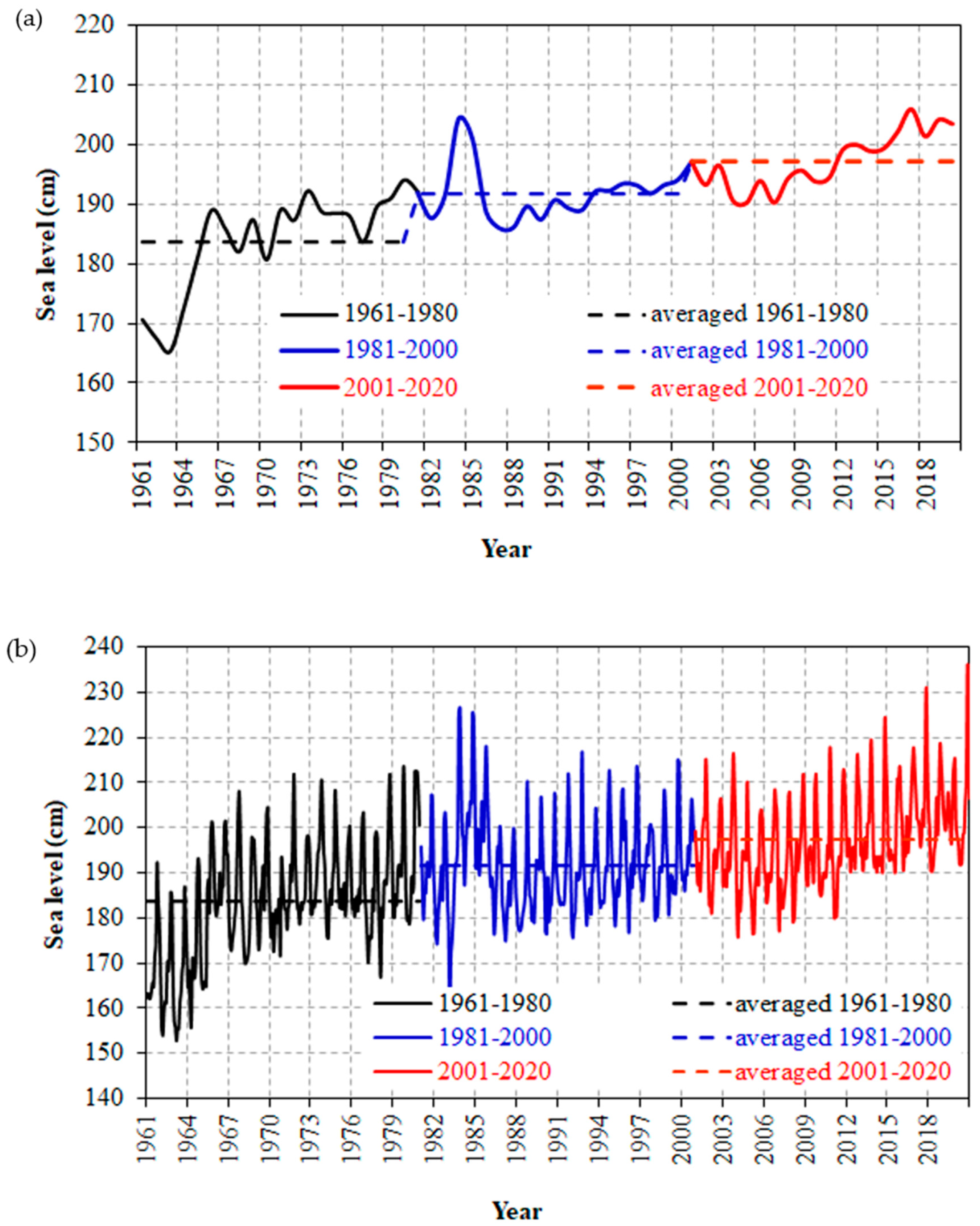
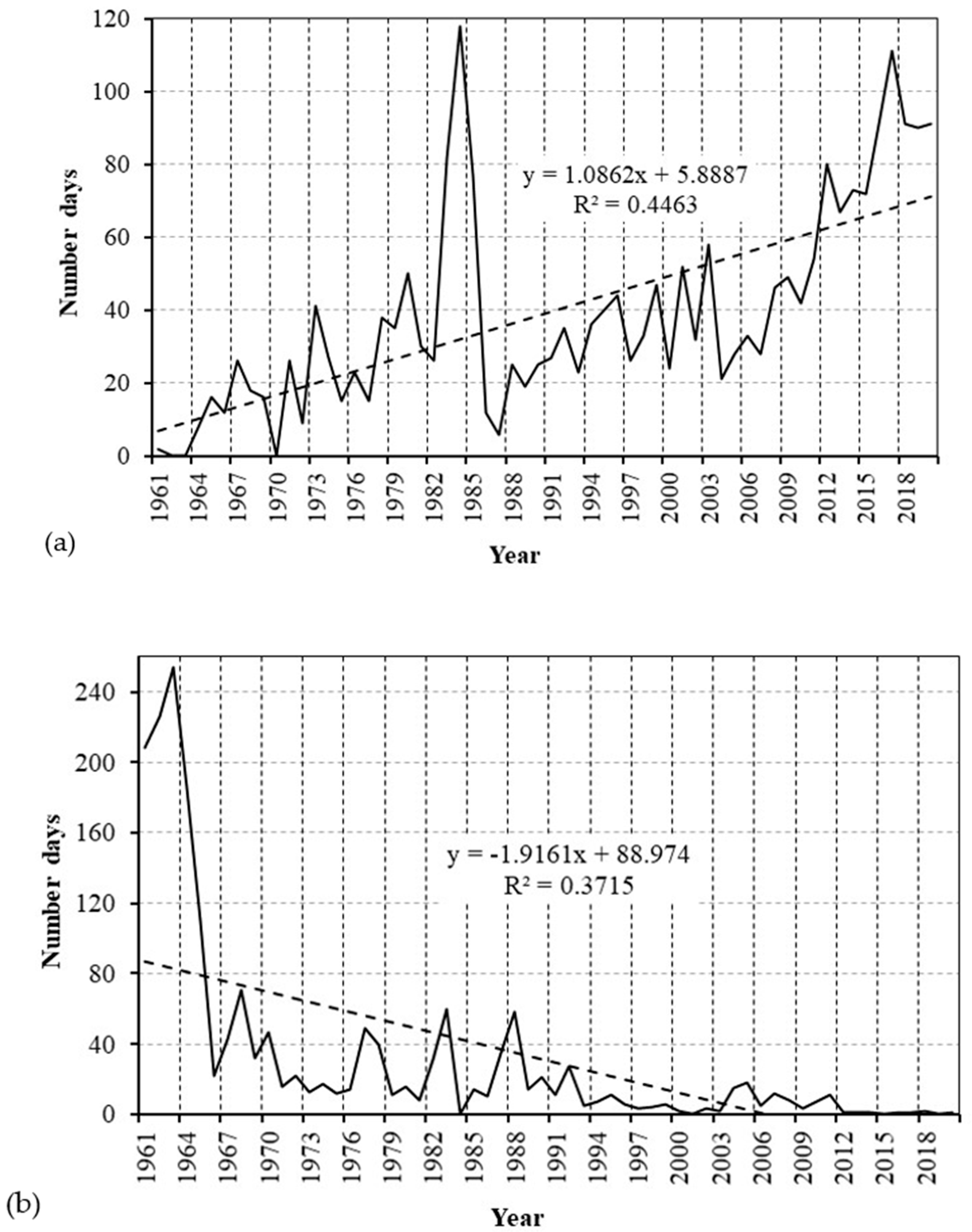
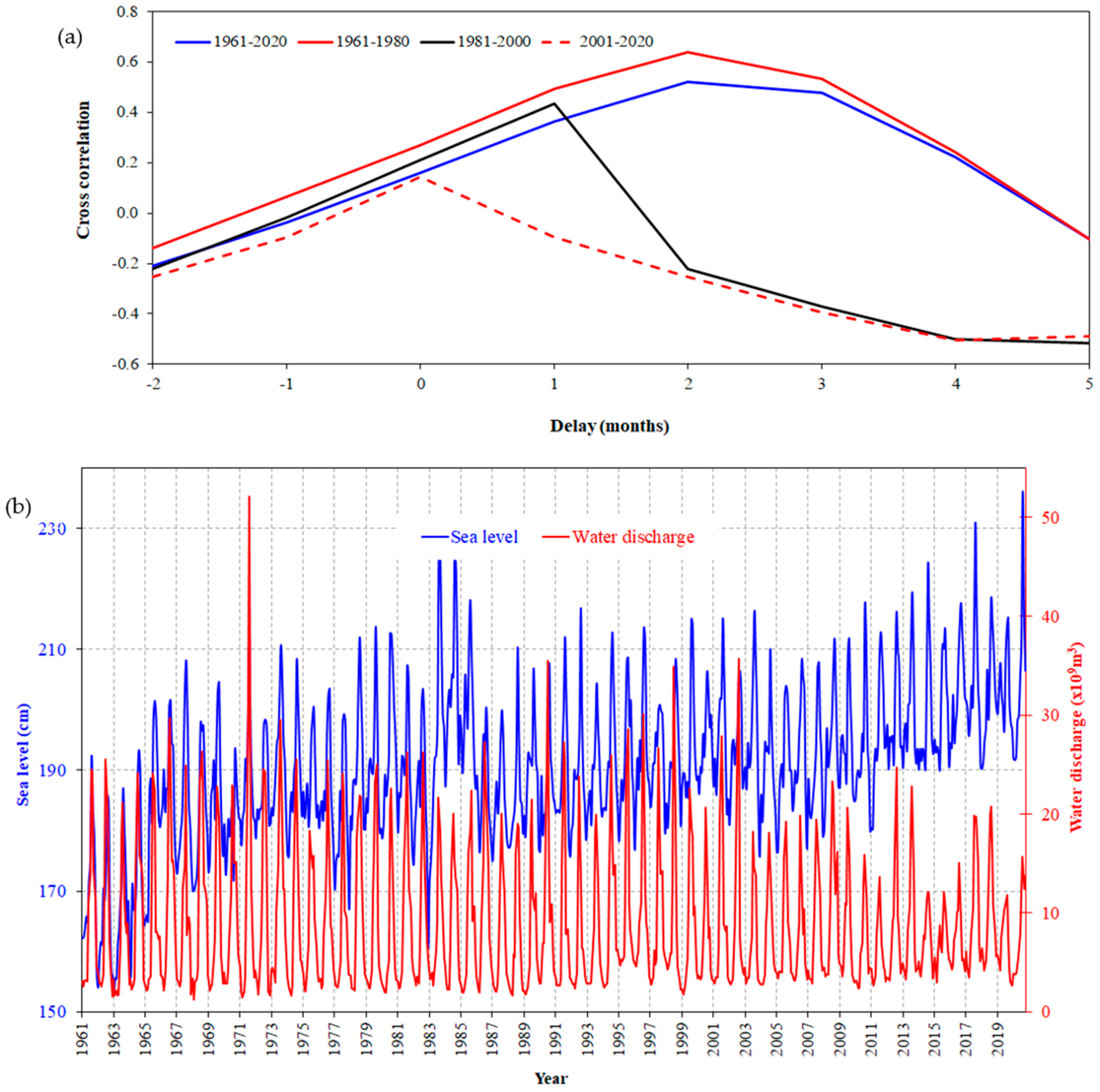
3.1. Temporal Variation of the Sea Level in Hai Phong Coastal Area for the Period 1961–2020

The annual sea level varied from 165.23 cm (in 1963) to 206.06 cm (in 2017) over the period 1961–2020. The average water level in this area was 190.86 cm for 60 years (1961–2020), which tended to be higher in recent years, especially from 2016 to the present, above 201.5 cm. The mean annual sea level in Hai Phong coastal area has changed in 60 years last: from 183.66 cm for 1961–1980 to 191.68 cm for 1981–2000 and reached 197.27 cm for 2001–2020 (Figure 3a). The annual sea levels in 1961–1978 were lower than average years, except 1973, then it increased and was higher than the average years in 1979–1985 (except in 1982) before decreasing under the average years in 1986–1993. From 1994 to 2020, the annual sea level was higher than the average years and reached a peak at 206.06 cm in 2017 (Figure 3a).

Before 1983, the monthly average water level was lower than the average value (190.86 cm), except for the last four months of the year (September, October, November, and December). However, since 1984, the monthly water level with a value higher than the average expanded to seven months: into the summer months (June, July, and August) to December. The lower value was in February and March, with 152.68–179.61 cm; then, they gradually increased in September–November (198–208 cm), reaching 208.26 cm in October (Figure 3b).

The results showed a significant increase in average monthly water levels in recent periods (Figure 3b). The number of months with an average water level higher than the average water level throughout the period (190.86 cm) has increased from 65 months for 1961–1980 to 112 months in 1981–2000, and 174 months for the period 2001–2020.

To assess the abnormal changes in water levels in the past, the number of days with an average water level value >210 cm and <170 cm was counted and shown in Figure 4. The results showed 2341 days with a mean sea level higher than 210 cm and 1832 days with a mean sea level less than 170 cm. In the periods 1961–2020, the number of days with mean sea level >210 cm also changed by the year. For example, there were only 98 days with a value higher than 210 cm for 1961–1970, but they increased to 279 days for 1971–1980. In particular, from 1981 to 1990, the number of days with an average water level >210 cm increased to 420 days. After this period, the number of days with higher sea levels decreased at 335 days for 1991–2000, then increased until recent years, with 389 days (2001–2010) and 820 days for 2011–2020. The number of days with an average level of 210 cm tended to increase for 1961–2020 (Figure 4a).

On the other hand, the number of days with sea level <170 cm was 1197 days for 1961–1970, accounting for about 65.3% of the total for 1961–2020. After this period, it decreased to 210 days for 1971–1980 and increased to 251 days for 1981–1990. Since 1991, the number of days tended to decline sharply: 82 days for 1991–2000, 73 days for 2001–2010, and 19 days for 2010–2020, and there were very few days in recent years (Figure 4b).

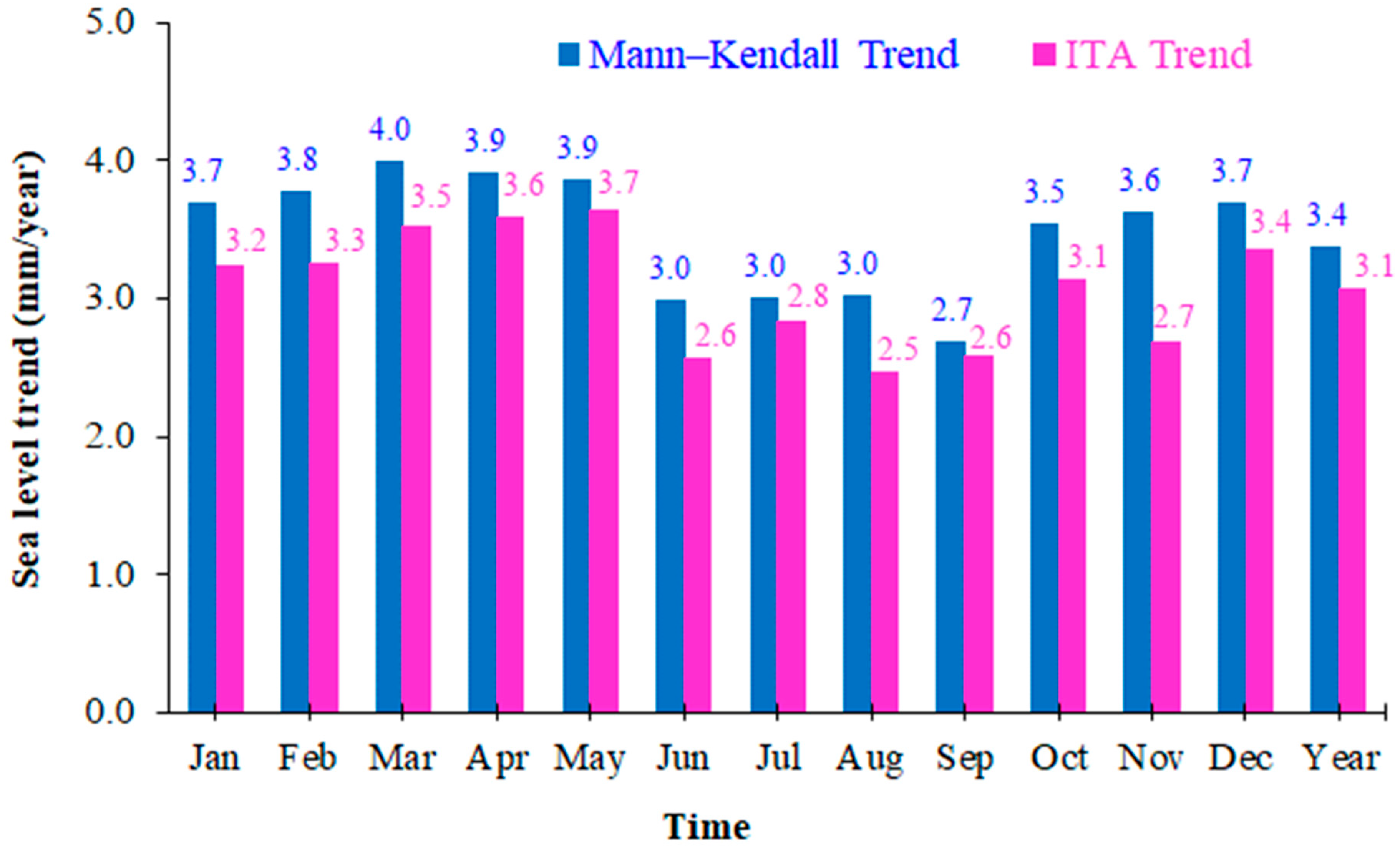
3.2. Mann–Kendall Trend Analysis

Based on the Mann–Kendall test, the sea level trend was calculated at the Hon Dau station for the different periods: 1961–1980, 1981–2000, 2001–2020, and 1961–2020, given in

Table 1. Trend analysis of sea level rise (mm/year) in the Hon Dau station using the Mann–Kendall test and Sen’s slope.

Months	Periods
	1961–2020		1961–1980		1981–2000		2001–2020
	p-Value	Slope	p-Value	Slope	p-Value	Slope	p-Value	Slope
1	0.00000	3.69	0.04781	8.17	0.58126	0.77 **	0.00025	9.20
2	0.00000	3.78	0.00255	10.36	0.41730	2.37 **	0.01248	7.03
3	0.00000	3.99	0.00165	12.95	0.06441	4.03 *	0.00708	7.7
4	0.00000	3.92	0.00255	11.47	0.45554	1.67 **	0.00708	7.29
5	0.00000	3.86	0.00041	13.91	0.16298	3.51 **	0.01496	5.06
6	0.00000	3.00	0.00255	10.38	0.82034	−0.69 **	0.00582	4.59
7	0.00000	3.00	0.00859	10.81	0.87113	0.09 **	0.01786	4.87
8	0.00000	3.03	0.00255	11.87	0.02518	8.49	0.11189	3.04 **
9	0.00001	2.68	0.02518	12.16	0.49566	1.56 **	0.00255	7.20
10	0.00000	3.55	0.00105	9.89	0.02518	8.49	0.00476	8.11
11	0.00000	3.63	0.00019	10.63	0.77029	1.55 **	0.00009	6.98
12	0.00000	3.70	0.02518	8.49	0.08552	5.96 *	0.01786	5.79
Year	0.00000	3.38	0.0002	10.33	0.08551	2.70 *	0.00015	7.16

* Statistically significant at 10% level; ** no significant trend.

. The p-values for all months were zero in 1961–2020, below the considered significance level of 99%. Therefore, the H₀ hypothesis is rejected, leading to the series’ statistical significance. The results showed a significant positive trend (Z > 0) for all months and 1961–2020. This means that sea level for all months in this period tended to rise along the Hai Phong coastal area. Using Sen’s approach, each time series’ sea level change (in mm per year) exhibits a statistically significant monotonic trend (Table 1). The monthly average rate from 1961 to 2020 was higher than 3.0 mm/year, except that in September (2.68 mm/year). While they were higher from March to May (transition season), with 3.86–3.99 mm/year, the lower value was 2.68 mm/year in September (rainy season). As a result, the rate of SLR in 1961–2020 was 3.38 mm/year.

As the period 1961–2020, in 1961–1980, the monthly average sea level also increased, with a 95–99% significance level. The monthly SLR varied from 8.17 mm/year to 13.91 mm/year, which was the highest compared to other periods. In this period, the highest and lowest values were 13.91 mm/year (May) and 8.17 mm/year (January), respectively. The average SLR in 1961–1980 was 10.33 mm/year, 6.95 mm/year higher than that in 1961–2020 (Table 1).

In 1981–2000, the p-value changed between 0.02518 and 0.87113, showing a 13–97.5% significance level. In this period, p values for all most months were higher than 0.1 (January, February, April, May, June, July, September, and November), illustrating no significant trend of these months. Only for 4 months (March, August, October, and December) were the p-values lower than 0.1, showing an increase of sea level with a confidence level of 90–95%. The rate of SLR for these months varied from 4.03 mm/year to 8.49 mm/year. In 1981–2000, the sea level increased with the lowest rate, at 2.7 mm/year (significance level of 90%) (Table 1).

During 2001–2020, the sea level increased, with 3.04–9.20 mm/year (significant level 89–99%). The highest monthly trend was observed in January, at 9.20 mm/year, while the lowest trend was in August, with a value of 3.04 mm/year (confident level of 89%). In 2001–2020, the average sea level rate held the second rank (after the period of 1961–1980), with 7.16 mm/year, which was about twice as great as it was in 1961–2020 (Table 1).

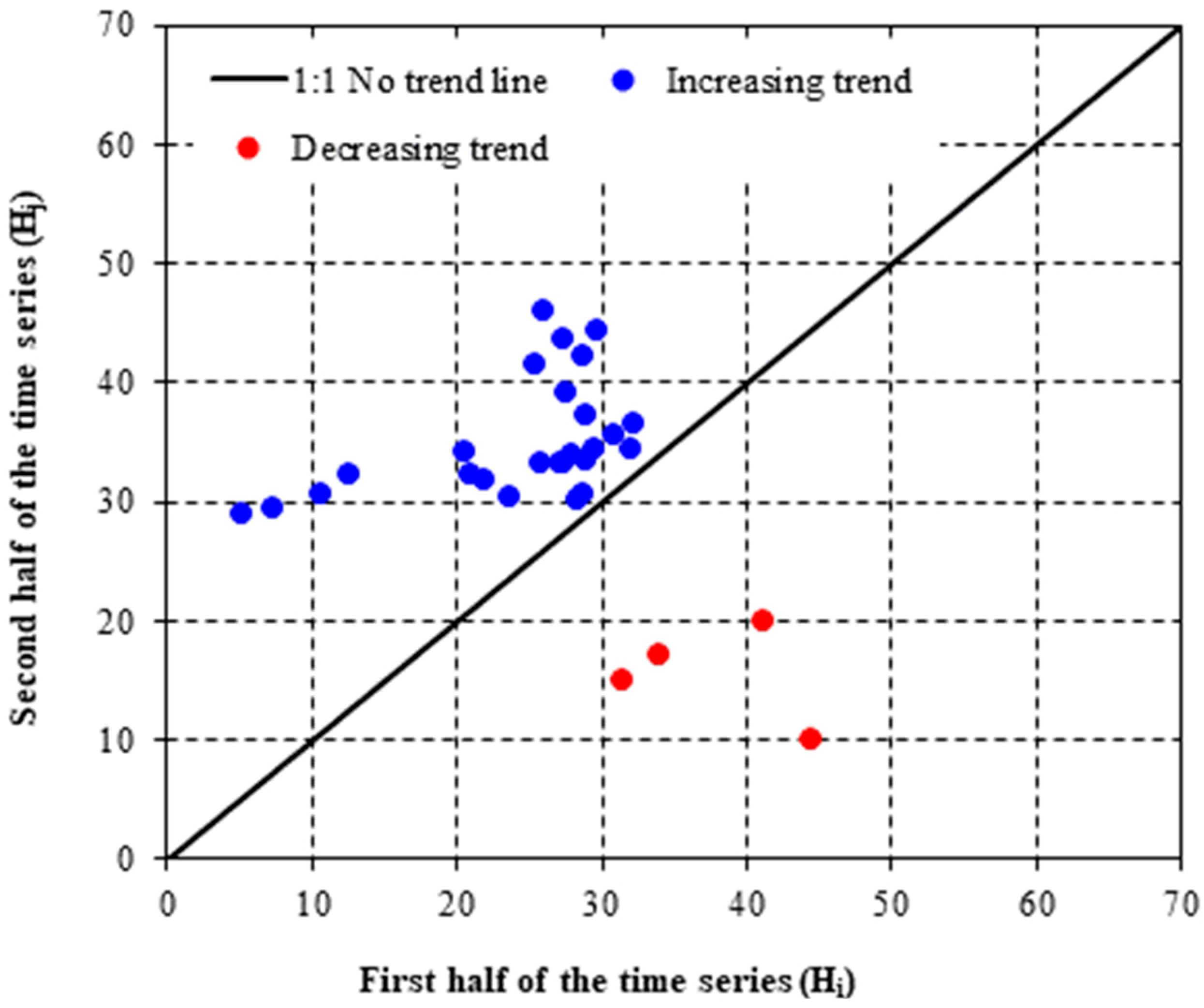
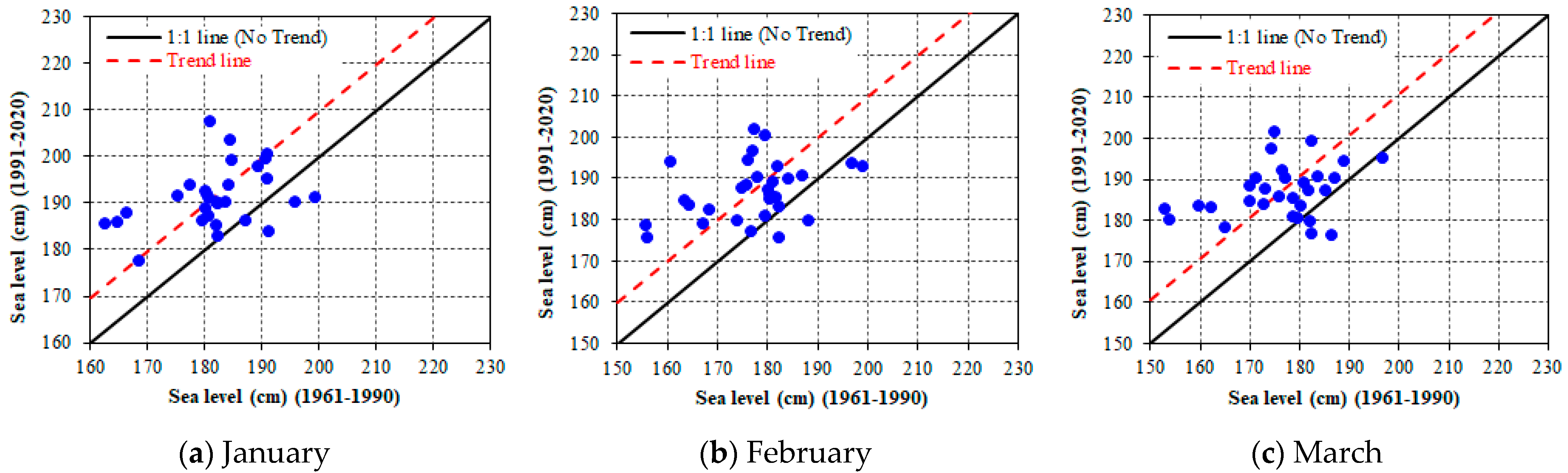
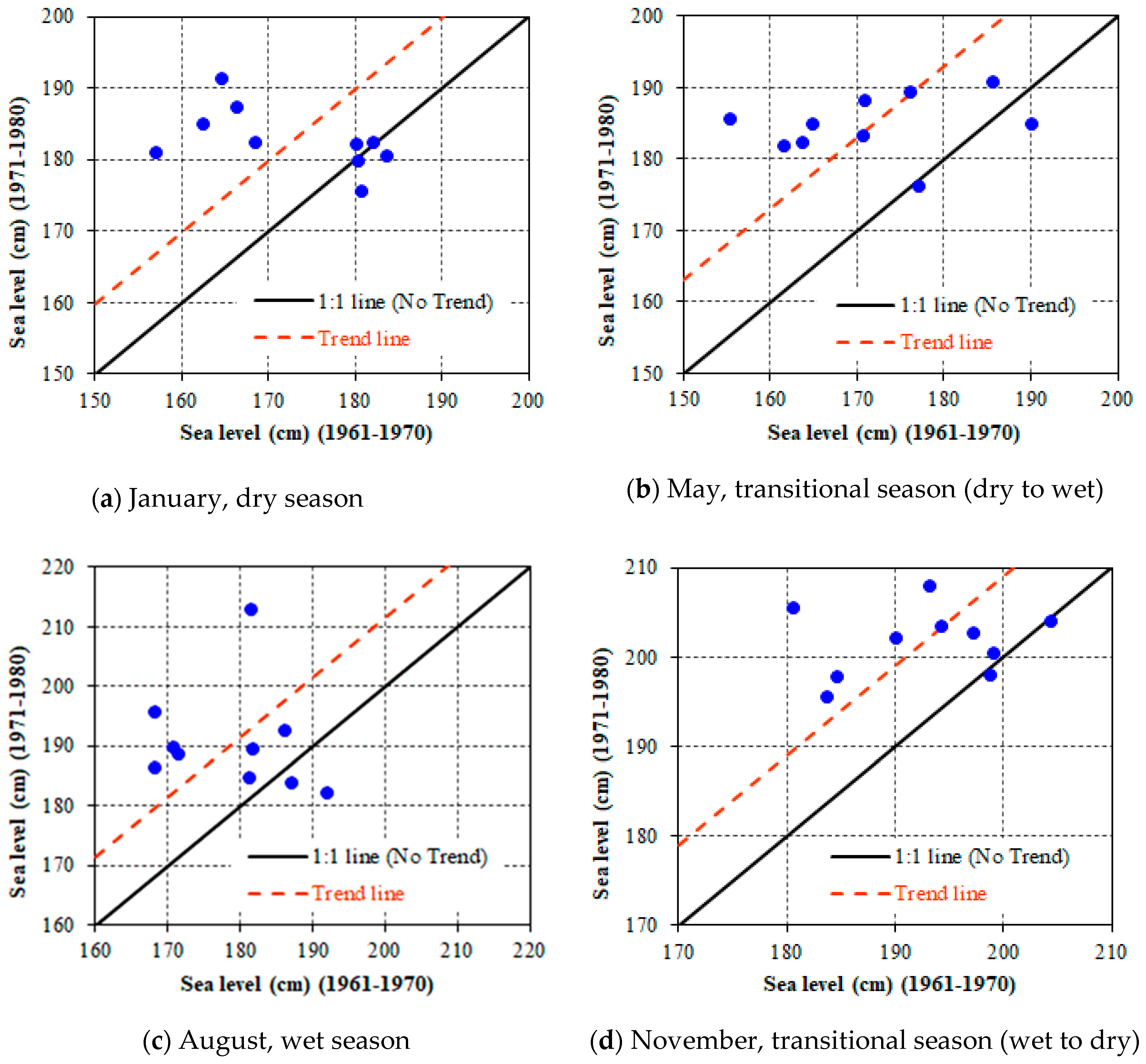
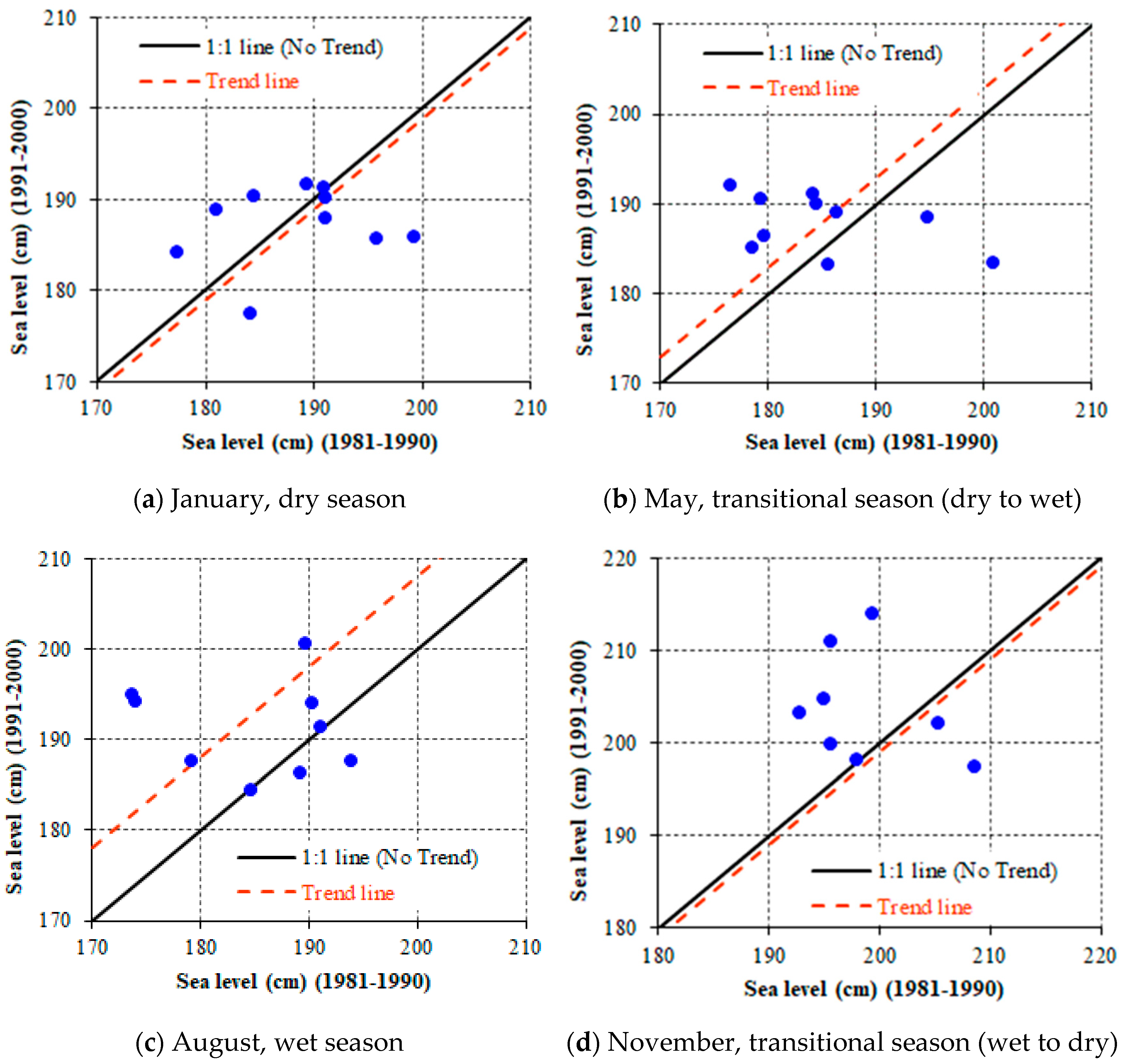
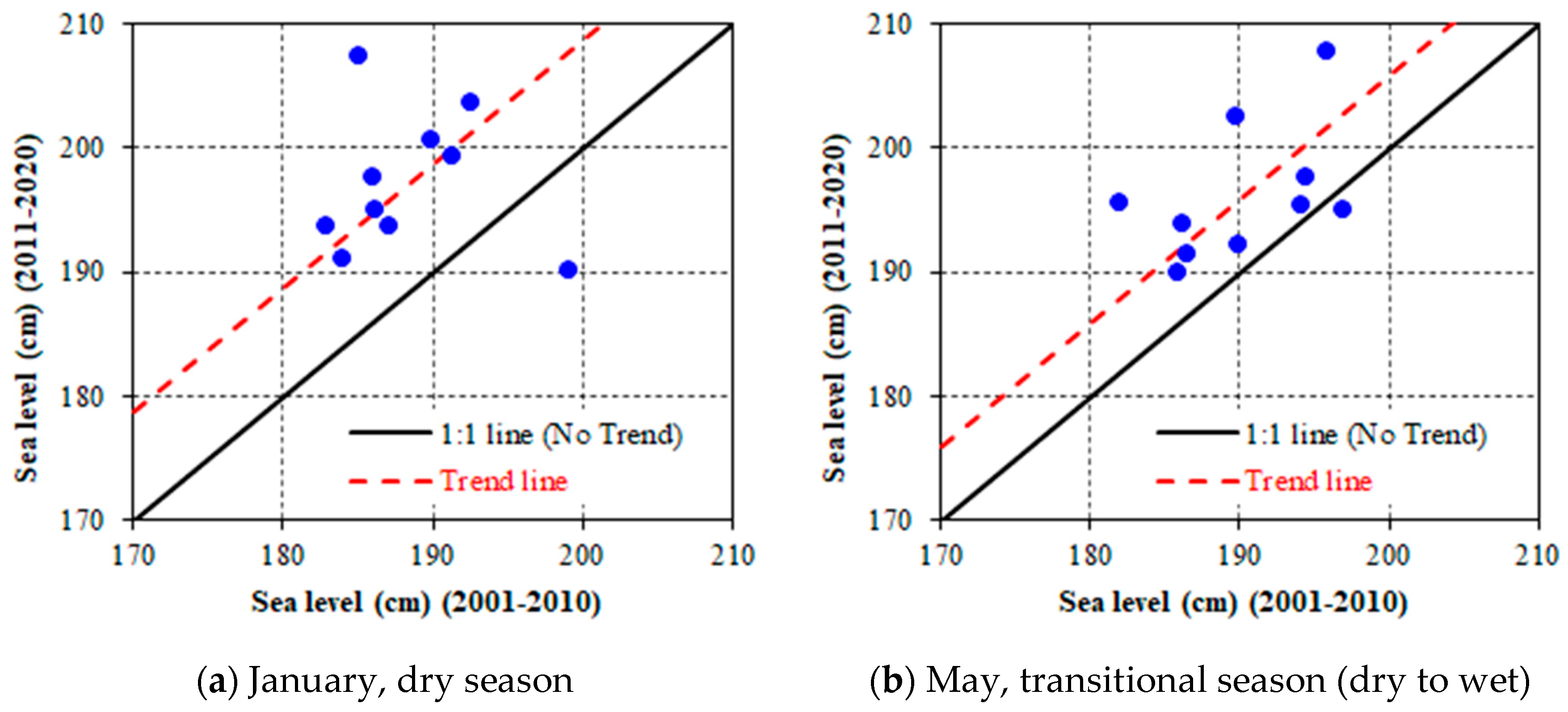
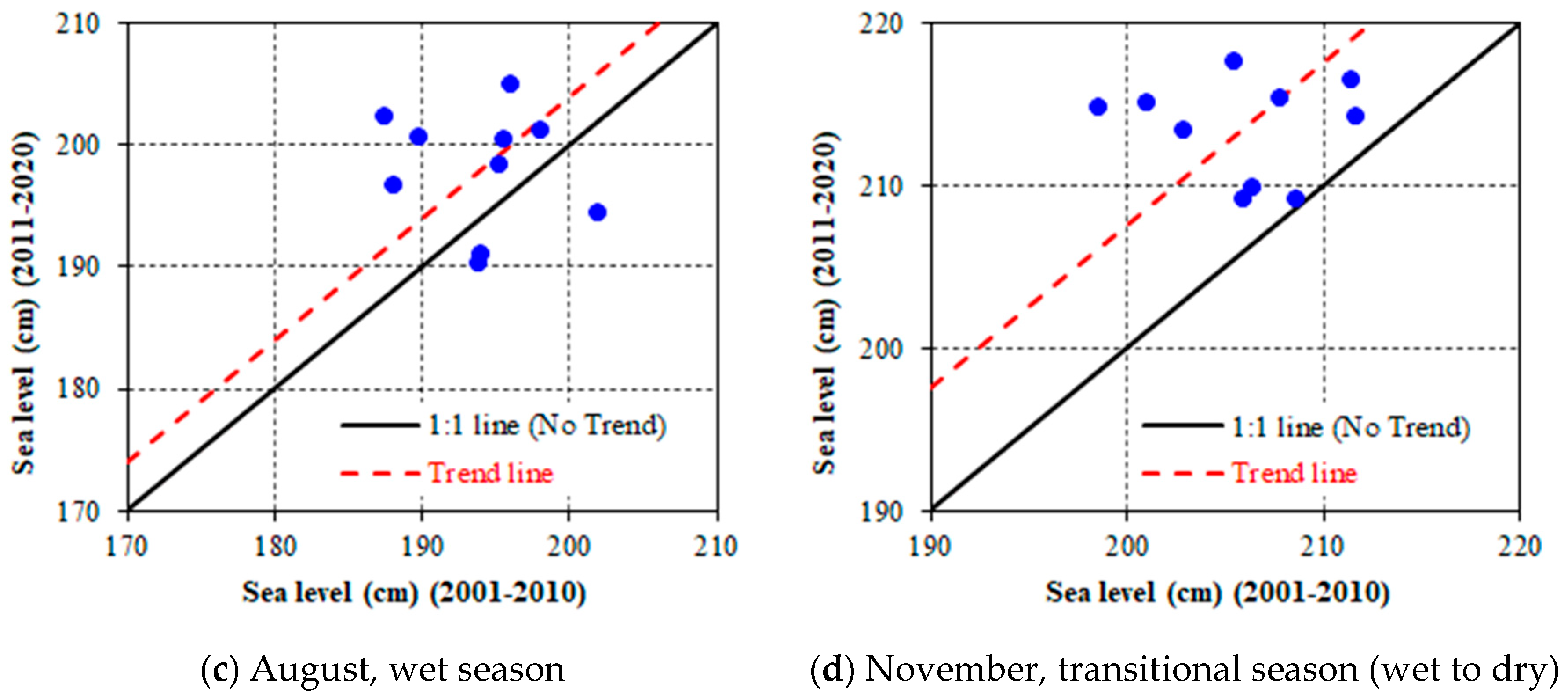
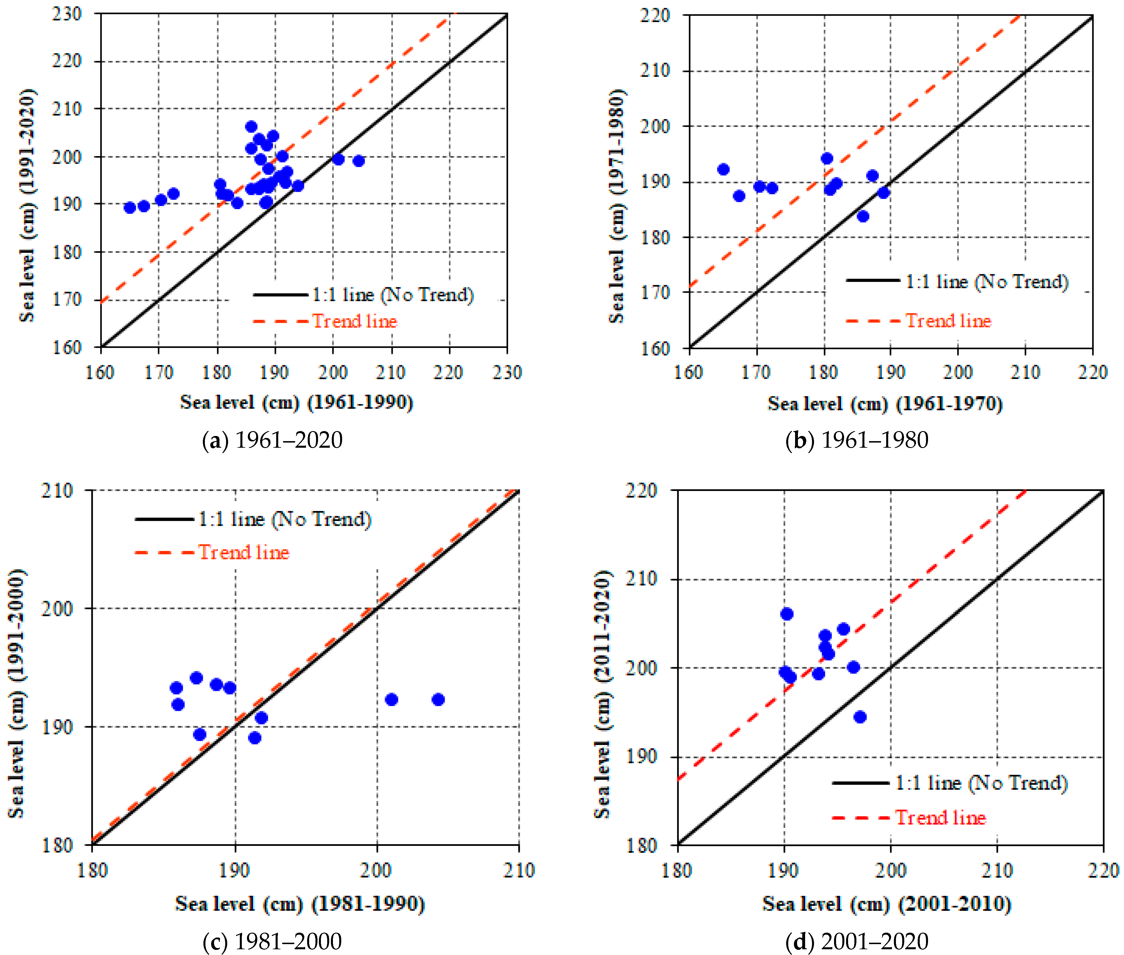
3.3. Innovative Trend Analysis (ITA) Method

For the period 1961–2020, the results of the ITA showed a significant positive pattern for all months with s > 0, and higher than CL (

Table 2. Trend analysis of SLR (mm/year) in the Hon Dau station using the ITA (s: slope, and CL: confidence limit, in mm/year).

Months/Time	Periods
	1961–2020		1961–1980		1981–2000		2001–2020
	s	CL	s	CL	s	CL	s	CL
1	3.25	±0.64	9.91	±2.76	−1.14 **	±2.51	8.81	±1.20
2	3.26	±0.50	10.54	±2.97	0.67 **	±1.62	9.03	±3.33
3	3.53	±0.48	12.99	±5.43	1.93 *	±1.78	8.59	±1.89
4	3.59	±0.56	12.63	±4.61	0.82 *	±0.78	7.19	±2.65
5	3.65	±0.75	12.96	±3.92	2.89	±2.41	6.00	±2.19
6	2.57	±0.55	10.84	±3.42	−3.22 **	±1.40	5.24	±0.80
7	2.84	±0.69	10.06	±0.92	0.61 **	±1.26	6.27	±0.43
8	2.48	±0.66	11.49	±2.15	8.12	±2.16	3.94	±1.80
9	2.59	±0.70	11.08	±2.31	2.96	±1.93	9.08	±1.53
10	3.14	±0.75	12.69	±2.58	8.12	±2.16	9.39	±2.59
11	2.69	±0.52	8.97	±2.32	−1.00 **	±3.13	7.58	±0.49
12	3.37	±0.71	8.12	±2.16	2.40 **	±3.46	7.42	±3.03
Year	3.08	±0.44	11.02	±1.45	0.50 **	±0.85	7.38	±1.81

* Statistically significant at 10% level; ** no significant trend.

). Monthly SLR in this period varied from 2.48 mm/year to 3.65 mm/year and tends to be higher (>3.25 mm/year) in the months from midwinter (December) to early summer (May) and smaller (<2.84 mm/year) during the summer months (Table 2). ITA monthly results are also illustrated in Figure 5. It is clear from the figure that an increasing trend and almost monotonic trend of the monthly.

The results of the ITA method for the subperiod 1961–1980 also showed a significant increasing trend for all months, and with a high rate compared with the period 1961–2020: around 8.12–9.91 mm/year in early to middle winter months (November to January). The increasing rate also was higher in the early summer months (March, April, May) and later summer months (August and September), with 11.08–12.99 mm/year (Table 2). The increasing trends of SLR of months in this subperiod mostly showed monotonic trends (Figure 6), like with the period 1961–2020 (Figure 5).

In 1981–2000, the monthly SLR trend was not steadied and differed from other periods. The declining trends in January, June, and November and the increasing trends in February, July, and December were not significant. The remaining months have an increasing trend with significance at 5–10%: March (1.93 mm/year); April (0.82 mm/year); May (2.89 mm/year); August (8.12 mm/year); September (2.96 mm/year); October (8.12 mm/year). Figure 7 showed nonmonotonic trends occurring in this period.

In the most recent 20 years (2001–2020), the ITA results showed a significant increasing trend for all months, around 4.0 to 6.27 mm/year for the summer months and 7.42–9.03 mm/year for the winter months (Table 2, Figure 8). The annual trends of sea level by the ITA method from 1961–2020 was 3.08 mm/year with significance at a 5% level (Table 2). The results of the ITA method for sea level time series data graphically from 1961 to 2020 are demonstrated in Figure 9a and showed a monotonic trend: increasing sea level in the range 190–205 cm. In subperiod 1961–1980, the trend with significance at 5% level, obtained from the ITA method, was 11.02 mm/year. The sea level time series data graphically in this period also showed a monotonic trend, with an increase of sea level around 190 cm (Figure 9b). On the other hand, the results from the ITA method for the period of 1981–2000 showed a trend with a close 1:1 line. The trend was not significant at 10% (CL = ±0.85 > s = 0.5, Table 2). This period’s graphical sea level data show a nonmonotonic distribution: the increasing sea level in 190–195 cm and the decrease in 200–205 cm (Figure 9c). In the most recent 20-year period, the SLR trend from the ITA method illustrated a rate of 7.38 mm/year (CL = ±1.81 with significance at 5% level, Table 2).

The SLA comparison results between measurement at the Hon Dau and AVISO data showed quite appropriate in the period 1993–2020. The correlation coefficient reached to 0.82. They fit well in 1998, 2001, 2002, 2003, and 2011–2013. Otherwise, the difference is greater in the years 1995, 2000, 2004, 2006, and 2007 (Figure 10a). It is noteworthy that after 2014 (2014–2020), the SLA at the Hon Dau station tended to be markedly higher than AVISO’s SLA from 2.6 to 6.1 cm.

Mean sea level trends are computed from measured data at the Hon Dau station and satellite altimetry data. The linear regression on moving average (over five years) evaluated the mean sea level trend for serial data from 1993 to 2020. The results showed that the trend changed from −16.61–15.84 mm/year (Hon Dau) and −9.13–14.94 mm/year (AVISO). The relationship between these trends also showed a relative agreement with a correlation coefficient of about 0.524, and the same decrease/increase tendency in 2002–2003, 2005–2007, and 2012–2015 (Figure 10b). However, the annual mean sea level rate from the AVISO data was significantly lower than tide gauge data during 2009–2017. The average trend rates from AVISO and the tide gauge data were 3.78 mm/year 4.92 mm/year, respectively, with a slight difference of 1.14 mm/year.

4. Discussion

4.1. The Variation of SLR Trend

In this study, the SLR trends at the Hon Dau station were analyzed using two different methods, over three successive 20-year periods. A confident, increasing sea level trend with lower values (3.38 mm/year by the Mann–Kendall test and Sen’s slope; and 3.08 mm/year by the ITA method) was found over the full 60-year period of 1961–2020, and higher values (7.16 mm/year by the Mann–Kendall test and Sen’s slope; and 7.38 mm/year by the ITA method) for recent years (2001–2020). These results are consistent with some previous studies. The SLR trend (by the Mann–Kendall test and Sen’s slope) over the period 1961–2020 was slightly lower than the result obtained by Ca [34] for the period 1957–2012 (3.78 mm/year). Our result was higher than the calculation obtained over the period 1960–2014 at the Hon Dau station (2.02 mm/year) and the average water level rise at all coastal stations of Vietnam in 1993–2014 (3.5 mm/year) [49]. In the same period, the mean SLR estimated by the AVISO (https://www.aviso.altimetry.fr/msl/, accessed on 10 February 2022) for global and North Pacific region scale was 3.33 mm/year and 2.85 mm/year, respectively. This shows that mean SLR in SCS increased faster than the global mean and the average over the North Pacific. For comparison purposes, we accessed mean sea level rise estimates by the AVISO for global and North Pacific region scale for 2001–2020. The global mean sea level acceleration results were 3.68 mm/year and about 3.24 mm/year for the North Pacific region, which was around twice lower than SLR in Hai Phong coastal area in our study (7.16 mm/year in 2001–2020).

The results showed a significant change of SLR in different periods based on the MK and Sen’s slope: 10.33 mm/year (1961–1980), 2.70 mm/year (1981–2000), and 7.16 mm/year (2001–2020) (Table 1). On the other hand, with the ITA method, the increasing sea level was 11.02 mm/year (1961–1980), 0.50 mm/year (1981–2000), and 7.38 mm/year (2001–2020) (Table 2). Global trends and nonclimate factors can explain the difference between the two periods. The highest trend of SLR occurred in 1961–1980, with 10–11 mm/year directly related to the rise of the annual water level from 1963 to 1966 (Figure 3b). It was consistent with the report that decadal trends in the global sea level reconstruction varied from 0 to 4 mm/year in 1950–2000, with a maximum during the 1970s [59]. On the global scale, according to the results of Church and White [60], the period of relatively rapid SLR commencing in the 1930s ceased abruptly in 1962, with decreasing of 10 mm over 5 years. In the late 1960s, the sea level rose about 2.4 mm/year for 15 years from 1967. This study removed direct factors (nonclimate) of anthropogenic change in terrestrial water storage (both dam storage and aquifer depletion) from their observations to focus on the sea level change related to climatic influences. Their resulting time series showed a slightly faster rate of sea level rise since about 1960. This is consistent with a noticeable increase in the average annual water level in the early 1960s of our study (Figure 3b).

Moreover, the hybrid sea level reconstruction during 1900–2015 combined previous techniques at time scales where they performed best. Dangendorf et al. [61] found a persistent acceleration in the global mean sea level since the 1960s, significantly (~76%) associated with sea level changes in the Indo-Pacific area. The initiation of the acceleration in the 1960s was tightly linked to intensification and a basin-scale equatorward shift of Southern Hemispheric westerlies, leading to increased ocean heat uptake and hence greater rates of global mean sea level rise. The increasing water level trend was the lowest in 1981–2000 with only 2.7 mm/year (by MK test and Sen’s slope) and 0.57 mm/year (by the ITA method). Our results are relatively consistent with Jevrejeva et al. [62], which showed the mean SLR rate in the West Pacific around 0–2.0 mm/year for 1980–2000. On a global scale, Church et al. [63] announced the increasing trend of SLR during the period 1980 to 2000, rising gradually from about 1.2 mm/year (1980) to 3.0 mm/year (2000).

From 2001 to the present (2020), the increasing SLR trend at the Hon Dau station showed a significant acceleration with about 7.16 mm/year (MK test and Sen’s slope) and 7.38 mm/year (ITA methods). These trends were twice higher than the trend for 1961–2020 (3.38 mm/year with MK test and Sen’s slope and 0.91 mm/year with ITA method, Table 1, Table 2). In addition, Church and White [60] reported a noticeable increase in the global mean sea level rate. While it only rose by about 1.6 mm/year in 1880–2009, it significantly increased in 1993–2009, with 3.2 ± 0.4 mm/year and 2.8 ± 0.8 mm/year from satellite altimetry and tide gauge data, respectively. The IPCC report [64] indicated that the global average SLR was 1.7 mm/year between 1901 and 2010, 2.0 mm/year between 1971 and 2010, and 3.2 mm/year between 1993 and 2010. The latest IPCC report [1] has updated these figures and indicated that the average rate of sea level rise had increased faster than expected in recent decades: 1.3 mm/year over 1901–1971, 1.9 mm/year over 1971–2006, and 3.7 mm/year for 2006–2018.

4.2. Factors Impacting the SLR Trends

The results in this study showed a similar increasing trend of sea level in recent years than at global scale [8,65,66,67]. However, regional sea level changes might differ substantially from a global average and show complex spatial patterns, resulting from ocean dynamical processes, lateral mass transport fluxes [68], and local changes in gravity [64]. For example, in the SCS region, Cheng and Qi [69] found the mean SLR at a rate of 11.3 mm/year during 1993–2000, and then a decreasing trend, with 11.8 mm/year during 2001–2005. On the other hand, Fu et al. [70] investigated the trend of SLR in SCS using the satellite altimetry and tide gauge data over 24 years (1993–2016) and reported a rise of +4.4 ± 0.3 mm/year (satellite data) and +3.9 ± 0.1 mm/year (tide gauge data).

The Hon Dau station locates about 10 km to the Van Uc River mouth and about 15 km from the Cam-Nam Trieu estuary. Therefore, water elevation may be influenced by fluvial water. The cross-correlation between monthly water discharge at Son Tay in the Red River (see [53]) and monthly sea level at the Hon Dau station was calculated to detect this relationship (Figure 11b). The sea level at the Hon Dau station tended to be higher with higher water discharge from the Red River. From 1961 to 2020, the maximum correlation between monthly water discharge from the Red River (at Son Tay) and monthly sea level at the Hon Dau station occurred after a two-month delay with a value of 0.52 (Figure 11a). It is noteworthy that there was a change in the maximum cross-correlation in periods: 0.63 with a delay of 2 months for 1961–1980; 0.43 with a 1-month delay for 1981–2000; and 0.14 without any delay for 2001–2020 (Figure 11a). This may be related to large reservoir dams upstream of the Red River system, especially the Hoa Binh Dam (which began construction on 6 November 1979, and was completed in December 1994), and to the resulting and irregular water regulation.

The water surges induced by typhoons in this area is another important factor on sea level. Statistics from the Vietnam Hydro-Meteorological Data and Information Center data, the Hai Phong coastal area has been impacted by 86 typhoons over 60 years (1961–2020), providing an average occurrence of about 1.43 typhoons/year. Among them, the number of big typhoons (maximum wind speed ≥ 11 category in Beaufort scale) tended to decrease in the periods 1961–1980, 1981–2000, and 2001–2020 with 9, 7, and 3 typhoons, respectively. The large number of big typhoons that occurred during the periods 1961–1980 and 1981–2000 may influence the trends of SLR. In particular, according to the statistics of the National Hydro-Meteorological Service, in the period 1961–2020, there were 11 seawater surges due to big typhoons in the Hai Phong area, especially in 1981–1990, in which 6 surges occurred (2 surges in 1981 and single surges in 1983, 1984, 1986, and 1989). During 1980–1990, there were 3 historic floods in the Red River Delta: the historical flooding in 1984 over 3 days was due to the most extreme rainfall over 100 years (1886 to 1997); the historical flooding in 1985 lasted 7 days, broke many sea dikes, and 78 people died; the historical flooding in 1986 over 15 days broke many dikes, 121 people died, banks collapsed, 491 houses drifted, and 12,571 homes were flooded. This may partly explain the higher average water levels in 1983–1986 (Figure 3) and influence the sea level trend during the periods 1981–2000. Moreover, since 1990, the effects of floods from the Red River to coastal areas almost have not occurred due to water regulation at the Hoa Binh dam [53]. Therefore, the trends of SLR in 2001–2020 were less noisy and more monotonic than in previous stages.

Like over other marine regions in the Pacific Ocean, the coastal area of Hai Phong in particular and the SCS, in general, are also clearly affected by the El Niño–Southern Oscillation (ENSO) phenomena, which is characterized by temperature and sea level anomalies in the tropical Pacific. This phenomenon affects global temperature, atmospheric pressure, and weather patterns and reflects large-scale atmosphere pressure fluctuations between the western and eastern tropical Pacific through the Walker circulation [71]. Therefore, sea level is one factor affected by ENSO [72,73,74,75]. Detrended global mean sea level changes are correlated to ENSO occurrences, with positive/negative sea level anomalies observed during El Niño/La Niña [76].

Based on the altimetry-derived sea level, tide gauge data, and the ENSO index, Rong et al. [77] showed a good correspondence of water level variation to ENSO and sea level in the SCS decreased during El Niño events and increased during La Niña events. Peng et al. [78] also found that the interannual variability of both observed and steric sea levels in SCS during the last 60 years (1950–2009) was driven by ENSO.

A lag is observed between sea level anomaly and ENSO index, which is locally dependent. In Moñitos, Cordoba (Colombian Caribbean Sea), the highest cross-correlation (0.65) between IMF4.5 and the ONI occurred after five months [79]. The contribution of ENSO to water level variation in this area is of around 8 cm, and the total sea level tended to be higher during El Niño phenomena and lower during La Niña events. On the contrary, also using the empirical mode decomposition (EMD) method, Wang et al. [80] found that the contribution of the ENSO phenomenon on interannual sea level variability in the Pearl River Estuary for 1953–2013 was around from −8.70 to 8.11 cm and found approximately 3–month lag. The maximum correlation of ONI and local sea level anomalies from the tide gauge station was 0.38. In the Pearl River Estuary, the sea level declined during El Niño events and rose during La Niña. Hai et al. [50] used the empirical mode decomposition method to identify the role of ENSO on the water level variability in 1960–2020. They showed that intrinsic mode functions (IMF) signal with the interannual periods of 2.0-years (IMF4) and 6.1- years (IMF5) were within the El Niño/La Niña (2–7 years). IMF4.5 was created from the sum of the IMF4 and IMF5 signals to represent the signal of sea-level response to ENSO. ENSO events took 4 months to impact the sea level in the Hai Phong coastal area, causing sea level variability within 20 cm for 1960–1971 and −3.7 to 7.2 cm for 1972–2020, with a cross-correlation of 0.27 (Figure 11). Hai et al. [50] also indicated that high sea levels occurred at some strong/extreme La Niña events (1973, 1975, 1998–99, and 2011).

Some previous studies reported higher levels during El Niño events and lower sea levels in La Niña events [76,79]. Meanwhile, higher sea levels also happened during the strong La Niña events, just like related studies in the western Pacific region [77,80]. In this study, the sea level was higher in some El Niño events (1963 (moderate), 1965, 1972, 1997 (very strong), and 2015 (weak)) and in some La Niña events (1973 (very strong), 1998, 2010 (strong), 1995, 2017 (moderate)). On the other hand, the sea level was also lower in El Niño events (1983 (very strong), 1992 (strong)) and La Niña events (1971 (moderate), 2008 (strong)). This showed that ENSO had influenced SLR, but it is not straightforward.

During the 1961–1980 period, the contribution of ENSO on the sea level at the Hon Dau station increased in El Niño events (1969, 1977) and strong La Niña events (1973, 1975) with a range of 0.6–10 cm. Those values were higher than the decreasing sea level in some La Niña events (1971, 1974, 1976, 1980), about −0.7 to −2.0 cm. From 1981 to 2000, sea level increased by ENSO was 0.3–3.5 cm in El Niño events (1986, 1991, 1998) and was fairly balanced with the decrease of sea level in this period from −0.4 to −3.8 cm during La Niña events (1983, 1989, 1990, 1998). However, ENSO’s contribution to the SLR was more pronounced between 2001 and 2020. The increasing values (2.2–7.2 cm) due to El Niño events (2004, 2014, 2019) were much greater than the decreasing values (−0.5 to −1.6 cm) due to La Niña events (2005, 2016). Note that an increase was observed in La Niña in 2011 and a decrease in El Niño 2009 as well.

4.3. Mann-Kendall and Şen’s Innovative Trend Method

The MK and ITA methods were both applied for the same sea level data at the Hon Dau station in this study. For a long period (1961–2020), a comparison of the results from the MK test and ITA methods demonstrated complete agreement among tests with significant rising trends. However, the trends of the MK method were higher than the ITA method (Figure 12): around 0.09 mm (3.7%) in September to 0.93 mm (34.37%) in November and 9.8% for annual values. The different results can be explained because the MK method calculates the trends as a median, so the contribution of extreme values to the trends may be ignored, while the trends in the ITA method are determined with the arithmetic mean of the first and second halves of the variable. Similar results were also observed in relevant previous studies [81,82,83,84].

Many previous studies reported the benefit of the ITA method over the trend detection by MK methods. MK is a nonparametric test that does not require data to be normally distributed and is not sensitive to outliers [85]. Moreover, Sen’s slope estimator is added to reinforce the MK test and calculate the trend according to the median value, reducing extreme values’ contribution to the trend component. Therefore, the trend results from the MK method sometimes do not reflect the reality when there are many extreme values in serial data. The MK is affected by serial correlations within the time series, which may lead to a disproportionate rejection of the null hypothesis of no trend whereas it is true [86]. Meanwhile, the ITA method does not include any assumptions (e.g., serial relationship, nonnormality, test number, etc.) and is not affected by serial correlation. ITA has a more powerful test for trend detection, which benefits from analyzing hidden variation trends of series that cannot be detected using traditional tests. It provides a visual–graphical illustration of trends, which helps to identify the trend of extreme events. In addition, the significant trends found by the ITA method are also often more prominent than the trends seen by the MK method. Their comparison over historical precipitation changes at 28 synoptic stations for 1946–2019 in Serbia by Arab Amiri and Gocić [87] showed that only three stations are recognized to be nonsignificant by the ITA method, while the MK test determined 16 stations with no significant trend. With measured temperature data for 1854 to 2017 at Oxford station in England, Alashan [83] found that the ITA method detected 11 monthly significant trends in the year, while the MK test gave 9. In our study, the ITA method found 7 nonsignificant trends (6 monthly in January, February, June, July, November, December, and the annual trend of the period 1981–2000), while the MK test gave 8 nonsignificant trends (except March, August, October, December, and annual of the period 1981–2000) (Table 1 and Table 2).

This can be explained in 1981–2000: the number of days with higher water level (>210 cm), which was 420 days in 1981–1990 decreased significantly in 1991–2000 (335 days). Moreover, during this period, the annual sea level in 1983–1985 was relatively high compared to other years (Figure 3a) with, in particular, 118 days with water levels higher than 210 cm in 1984 (highest in the period 1961–2020, Figure 4a), and without day with water levels lower than 170 cm (Figure 4b). On the other hand, although the sea level rose from 1988–2000, the average water level in 1991–2000 compared to 1981–1990 did not differ significantly (only 0.5 cm, Table 2). The results of the ITA method confirmed the nonmonotonic trend for the 1981–2000 (Figure 9). Therefore, the nonmonotonic trends occurred in the results of the annual trend analysis and appeared in the monthly trends for the period 1981–2000 (Figure 7). This is the reason for the different trends between the MK test and ITA method. This has been confirmed in previous related studies [83,87,88,89]. In addition, the results of analysis from the ITA method also showed that in the period 1981–2000, nonmonotonic monthly trends appear more pronounced than the analysis in 1961–1980 (Figure 6) and 2001–2020 (Figure 8).

5. Conclusions

The variation trends of annual and monthly sea level at the Hon Dau station, Hai Phong coastal area, and Vietnam during 1961–2020 were analyzed using MK test with Sen’s slope estimator and ITA method. Additionally, the trends of subperiods (1961–1980, 1981–2000, 2001–2020) were detected using both ways to evaluate the reliability of these methods. The results showed that the annual sea level varied from 165.23 cm to 206.06 cm in 1961–2020. The average water level was 190.87 cm for 60 years (1961–2020), which tended to be higher in recent years, especially from 2016 to the present, above 202 cm. This area’s mean annual sea level has changed in 60 years last: from 183.66 cm for 1961–1980 to 191.68 cm for 1981–2000 and reached 197.27 cm for 2001–2020. It should be noted that the number of days with a mean sea level higher than 210 cm has increased since the 1960s: only 98 days in the period 1961–1970, 279 days for 1971–1980, and 820 days for 2011–2020.

Both the results from the MK test and ITA method confirmed the positive trend of SLR at the Hai Phong coastal area in the period 1961–2020. Comparisons between the MK test and ITA method demonstrated complete agreement among tests with significant rising trends of about 3.38 mm/year and 3.08 mm/year, respectively. However, both ways provided similar results only for periods: 1961–2020, 1961–1980, and 2001–2020, with relatively stable monotonic related trend conditions. For the period 1981–2000, with the appearance of a more nonmonotonic trend, gave different trends between methods, which shows the benefits of ITA when it allows more detailed interpretations about trend detection. One main advantage is that it does not have any assumptions (e.g., serial correlation, non-normality, sample number, etc.) as in the MK method. Moreover, the trends can be detected at different sea level series, which provides reliable tendencies for future prediction of SLR.

This study presented a comprehensive investigation of the temporal variation of monthly sea level in the Hai Phong coastal area between 1961 and 2020. The results are helpful for managers involved in predicting the risk associated with SLR in the study area. This study also contributes to the trend detection methods by quantitatively evaluating trends in the data range value groups of time series. However, our study focuses only on interannual sea level trends at Hon Dau tidal gauge station. Future research will collect more tidal gauge station data to examine temporal variation and spatial variation of sea level along the coasts of Vietnam.

References

1. IPCC. Climate Change 2021: The Physical Science Basis. Contribution of Working Group I to the Sixth Assessment Report of the Intergovernmental Panel on Climate Change; Masson-Delmotte, V., Zhai, P., Pirani, A., Connors, S.L., Péan, C., Berger, S., Caud, N., Chen, Y., Goldfarb, L., Gomis, M.I., et al., Eds.; Cambridge University Press: Cambridge, UK, 2021. [Google Scholar]
2. Fitzgerald, D.M.; Fenster, M.S.; Argow, B.A.; Buynevich, I.V. Coastal impacts due to sea level rise. Annu. Rev. Earth Planet. Sci. 2008, 36, 601–647. [Google Scholar] [CrossRef] [Green Version]
3. Nicholls, R.J.; Cazenave, A. Sea-level rise and its impact on coastal zones. Science 2010, 328, 1517–1520. [Google Scholar] [CrossRef] [PubMed]
4. Small, C.; Nicholls, R.J. A global analysis of human settlement in coastal zones. J. Coast. Res. 2003, 19, 584–599. Available online: https://www.jstor.org/stable/4299200 (accessed on 15 December 2021).
5. Nicholls, R.J.; Wong, P.P.; Burkett, V.R.; Codignotto, J.O.; John, H.; McLean, R.F.; Ragoonaden, S.; Woodroffe, C.D. Coastal systems and low-lying areas, in Climate Change 2007: Impacts, Adaptation, and Vulnerability. In Contribution of Working Group II to the Fourth Assessment Report of the Intergovernmental Panel on Climate Change; Parry, M.L., Canziani, O.F., Palutikof, J.P., van der Linden, P.J., Hanson, C.E., Eds.; Cambridge University Press: Cambridge, UK, 2007; p. 976. [Google Scholar]
6. Anthoff, D.; Nicholls, R.J.; Tol, R.S.J.; Vafeidis, A.T. Global and Regional Exposure to Large Rises in Sea-Level: A Sensitivity Analysis; (Working Paper: 96); Tyndall Centre for Climate Change Research: Norwich, UK, 2006; p. 31. [Google Scholar]
7. Almeida, B.A.; Mostafavi, A. Resilience of infrastructure systems to sea-level rise in coastal areas: Impacts, adaptation measures, and implementation challenges. Sustainability 2016, 8, 1115. [Google Scholar] [CrossRef] [Green Version]
8. Church, J.A.; Clark, P.U.; Cazenave, A.; Gregory, J.M.; Jevrejeva, S.; Levermann, A.; Merrifield, M.A.; Milne, G.A.; Nerem, R.S.; Nunn, P.D.; et al. Sea Level Change in Climate Change 2013: The Physical Science Basis. Contribution of Working Group I to the Fifth Assessment Report of the Intergovernmental Panel on Climate Change; Stocker, T.F., Qin, D., Plattner, G.-K., Eds.; Cambridge University Press: Cambridge, UK, 2013; pp. 1137–1216. [Google Scholar] [CrossRef] [Green Version]
9. Baede, A.P.M. Annex I glossary. In Climate Change 2007: The Physical Science Basis. Contribution of Working Group I to the Fourth Assessment Report of the Intergovernmental Panel on Climate Change; Solomon, S., Qin, D., Manning, M., Chen, Z., Marquis, M., Averyt, K.B., Tignor, M., Miller, H.L., Eds.; Cambridge University Press: Cambridge, UK, 2007; pp. 941–954. [Google Scholar]
10. Milne, G.A.; Gehrels, W.R.; Hughes, C.W.; Tamisiea, M.E. Identifying the causes of sea-level change. Nature Geosci. 2009, 2, 471–478. [Google Scholar] [CrossRef] [Green Version]
11. Ying, Q.; Svetlana, J.; Luke, P.J.; John, C.M. Coastal sea level rise around the China Seas. Glob. Planet. Chang. 2019, 171, 454–463. [Google Scholar] [CrossRef]
12. Li, L.; Xu, J.; Cai, R. Trends of sea level rise in the South China Sea during the 1990s: An altimetry result. Chin. Sci. Bull. 2002, 47, 582–585. [Google Scholar] [CrossRef]
13. Sen, P.K. Estimates of the Regression Coefficient Based on Kendall’s Tau. J. Am. Stat. Assoc. 1968, 63, 1379. [Google Scholar] [CrossRef]
14. Hirsch, R.M.; Slack, J.R. A nonparametric trend test for seasonal data with serial dependence. Water Resour. Res. 1984, 20, 727–732. [Google Scholar] [CrossRef] [Green Version]
15. Duan, Z.; Tuo, Y.; Liu, J.; Gao, H.; Song, X.; Zhang, Z. Hydrological evaluation of open-access precipitation and air temperature datasets using SWAT in a poorly gauged basin in Ethiopia. J. Hydrol. 2019, 569, 612–626. [Google Scholar] [CrossRef] [Green Version]
16. Gao, H.; Birkel, C.; Hrachowitz, M.; Tetzlaff, D.; Soulsby, C.; Savenije, H.H.G. A simple topography-driven and calibration-free runoff generation module. Hydrol. Earth Syst. Sci. 2019, 23, 787–809. [Google Scholar] [CrossRef] [Green Version]
17. Dong, J.; Crow, W.T.; Duan, Z.; Wei, L.; Lu, Y. A double instrumental variable method for geophysical product error estimation. Remote Sens. Environ. 2019, 225, 217–228. [Google Scholar] [CrossRef] [Green Version]
18. Hamed, K.H.; Rao, A.R. A modified Mann-Kendall trend test for autocorrelated data. J. Hydrol. 1998, 204, 182–196. [Google Scholar] [CrossRef]
19. Hamed, K.H. Improved finite-sample Hurst exponent estimates using rescaled range analysis. Water Resour. Res. 2007, 43, 797–809. [Google Scholar] [CrossRef]
20. Öztopal, A.; Şen, Z. Innovative Trend Methodology Applications to Precipitation Records in Turkey. Water Resour. Manag. 2017, 31, 727–737. [Google Scholar] [CrossRef]
21. Wu, H.; Qian, H. Innovative trend analysis of annual and seasonal rainfall and extreme values in Shaanxi, China, since the 1950s. Int. J. Climatol. 2017, 37, 2582–2592. [Google Scholar] [CrossRef]
22. Kisi, O. An innovative method for trend analysis of monthly pan evaporations. J. Hydrol. 2015, 527, 1123–1129. [Google Scholar] [CrossRef]
23. Shadmani, M.; Marofi, S.; Roknian, M. Trend Analysis in Reference Evapotranspiration using Mann-Kendall and Spearman’s rho tests in arid regions of Iran. Water Resour. Manag. 2012, 26, 211–224. [Google Scholar] [CrossRef] [Green Version]
24. Helsel, D.; Hirsch, R. Statistical Methods in Water Resources; Studies in Environmental Science Series; Elsevier: Amsterdam, The Netherlands, 1992; Volume 49, 522p. [Google Scholar]
25. Hirsch, R.M.; Slack, J.R.; Smith, R.A. Techniques of trend analysis for monthly water quality data. Water Resour. Res. 1982, 18, 107–121. [Google Scholar] [CrossRef] [Green Version]
26. Burn, D.H.; Hannaford, J.; Hodgkins, G.A.; Whitfield, P.H.; Thorne, R.; Marsh, T. Reference hydrologic networks II. using reference hydrologic networks to assess climate-driven changes in streamflow. Hydrol. Sci. J. 2012, 57, 1580–1593. [Google Scholar] [CrossRef] [Green Version]
27. Douglas, E.M.; Vogel, R.M.; Kroll, C.N. Trends in floods and low flows in the United States: Impact of spatial correlation. J. Hydrol. 2000, 240, 90–105. [Google Scholar] [CrossRef]
28. Serinaldi, F.; Kilsby, C.G.; Lombardo, F. Untenable nonstationarity: An assessment of the fitness for purpose of trend tests in hydrology. Adv. Water Resour. 2018, 111, 132–155. [Google Scholar] [CrossRef]
29. Chebana, F.; Aissia, M.A.B.; Ouarda, T.B.M.J. Multivariate shift testing for hydrological variables, review, comparison and application. J. Hydrol. 2017, 548, 88–103. [Google Scholar] [CrossRef] [Green Version]
30. Sang, Y.F.; Wang, Z.; Liu, C. Comparison of the MK test and EMD method for trend identification in hydrological time series. J. Hydrol. 2017, 510, 293–298. [Google Scholar] [CrossRef]
31. Wang, S.; Zuo, H.; Yin, Y.; Hu, C.; Yin, J.; Ma, X. Interpreting rainfall anomalies using rainfall’s nonnegative nature. Geophys. Res. Lett. 2019, 46, 426–434. [Google Scholar] [CrossRef] [Green Version]
32. Wahl, T.; Jensen, J.; Frank, T.; Haigh, I.D. Improved estimates of mean sea level changes in the German Bight over the last 166 years. Ocean Dyn. 2011, 61, 701–715. [Google Scholar] [CrossRef]
33. Chandler, R.E.; Scott, E.M. Statistical Methods for Trend Detection and Analysis in the Environmental Sciences; John Wiley: Chichester, UK, 2011; 392p. [Google Scholar]
34. Ca, V.T. A Climate Change Assessment via Trend Estimation of Certain Climate Parameters with In Situ Measurement at the Coasts and Islands of Viet Nam. Climate 2017, 5, 36. [Google Scholar] [CrossRef]
35. Ozgenc Aksoy, A. Investigation of sea level trends and the effect of the north atlantic oscillation (NAO) on the black sea and the eastern mediterranean sea. Theor. Appl. Climatol. 2017, 129, 129–137. [Google Scholar] [CrossRef]
36. Su, B.; Jiang, T.; Jin, W. Recent trends in observed temperature and precipitation extremes in the Yangtze River basin, China. Theor. Appl. Climatol. 2006, 83, 139–151. [Google Scholar] [CrossRef]
37. Wang, Y.; Wang, D.; Lewis, Q.W.; Wu, J.; Huang, F. A framework to assess the cumulative impacts of dams on hydrological regime: A case study of the Yangtze River. Hydrol. Processes 2017, 31, 3045–3055. [Google Scholar] [CrossRef]
38. Zhang, Q.; Xu, C.Y.; Zhang, Z.; Chen, Y.D.; Liu, C.L.; Lin, H. Spatial and temporal variability of precipitation maxima during 1960–2005 in the Yangtze River basin and possible association with large-scale circulation. J. Hydrol. 2008, 353, 215–227. [Google Scholar] [CrossRef]
39. Dabanlı, İ.; Şen, Z.; Yeleğen, M.; Şişman, E.; Selek, B.; Guclu, Y. Trend assessment by the innovative-Şen method. Water Resour. Manag. 2016, 30, 1–11. [Google Scholar] [CrossRef]
40. Şen, Z. Innovative trend analysis methodology. J. Hydrol. Eng. 2012, 17, 1042–1046. [Google Scholar] [CrossRef]
41. Sonali, P.; Kumar, D. Review of trend detection methods and their application to detect temperature changes in India. J. Hydrol. 2013, 476, 212–227. [Google Scholar] [CrossRef]
42. Tabari, H.; Taye, M.T.; Onyutha, C.; Willems, P. Decadal analysis of river flow extremes using quantile-based approaches. Water Resour. Manag. 2017, 31, 3371–3387. [Google Scholar] [CrossRef]
43. Zhou, Z.; Wang, L.; Lin, A.; Zhang, M.; Niu, Z. Innovative trend analysis of solar radiation in China during 1962–2015. Renew. Energy 2018, 119, 675–689. [Google Scholar] [CrossRef]
44. Ay, M.; Kisi, O. Investigation of trend analysis of monthly total precipitation by an innovative method. Theor. Appl. Climatol. 2014, 120, 617–629. [Google Scholar] [CrossRef]
45. Dasgupta, S.; Laplante, B.; Meisner, C. The impact of sea level rise on developing countries: A comparative analysis. Clim. Chang. 2009, 93, 379–388. [Google Scholar] [CrossRef]
46. IPCC. Climate Change 2007: The Physical Science Basis. Contribution of Working Group I to the Fourth Assessment Report of the Intergovernmental Panel on Climate Change; Solomon, S., Qin, D., Manning, M., Chen, Z., Marquis, M., Averyt, K.B., Tignor, M., Miller, H.L., Eds.; Cambridge University Press: Cambridge, UK; New York, NY, USA, 2007; p. 996. [Google Scholar]
47. A.D.B. Vietnam: Environment and Climate Change Assessment. 2013. Available online: https://www.adb.org/documents/viet-nam-environment-and-climate-change-assessment (accessed on 6 August 2021).
48. Tuong, N.T. Sea Level Measurement and Sea Level Rise in Vietnam; Marine Hydrometeorological Centre: Hanoi, Vietnam, 2006. [Google Scholar]
49. MONRE. Climate Change and Sea Level Rise Scenarios for Viet Nam; The Ministry of Natural Resources and Environment: Hanoi, Vietnam, 2016; 169p. [Google Scholar]
50. Hai, N.M.; Ouillon, S.; Vinh, V.D. Sea level rise in Hai Phong coastal area (Vietnam) and its response to Enso—Evidence from tide gauge measurement of 1960–2020. Vietnam J. Earth Sci. 2022, 44, 109–126. [Google Scholar] [CrossRef]
51. Vinh, V.D.; Ouillon, S. The double structure of the Estuarine Turbidity Maximum in the Cam-Nam Trieu mesotidal tropical estuary, Vietnam. Mar. Geol. 2021, 442, 106670. [Google Scholar] [CrossRef]
52. Vinh, V.D.; Ouillon, S.; Uu, D.V. Estuarine Turbidity Maxima and Variations of Aggregate Parameters in the Cam-Nam Trieu Estuary, North Vietnam, in Early Wet Season. Water 2018, 10, 68. [Google Scholar] [CrossRef] [Green Version]
53. Vinh, V.D.; Ouillon, S.; Thanh, T.D.; Chu, L.V. Impact of the Hoa Binh dam (Vietnam) on water and sediment budgets in the Red River basin and delta. Hydrol. Earth Syst. Sci. 2014, 18, 3987–4005. [Google Scholar] [CrossRef] [Green Version]
54. Vinh, V.D.; Ouillon, S.; Hai, N.M. Sea surface temperature trend analysis by Mann-Kendall test and Sen’s slope estimator: A study of the Hai Phong coastal area (Vietnam) for the period 1995–2020. Vietnam J. Earth Sci. 2022, 44, 72–91. [Google Scholar] [CrossRef]
55. NOAA. 2020. Available online: https://origin.cpc.ncep.noaa.gov/products/analysis_monitoring/ensostuff/ONI_v5.php (accessed on 31 December 2020).
56. Theil, H. A rank-invariant method of linear and polynomial regression analysis I, II and III. Nederl. Aka. Wetensch 1950, 53, 386–392. [Google Scholar]
57. Elouissi, A.; Şen, Z.; Habi, M. Algerian rainfall Innovative trend analysis and its implications to Macta watershed. Arab. J. Geosci. 2016, 9, 303. [Google Scholar] [CrossRef]
58. Şen, Z. Innovative trend significance test and applications. Theor. Appl. Climatol. 2017, 127, 939–947. [Google Scholar] [CrossRef]
59. White, N.J.; Church, J.A.; Gregory, J.M. Coastal and global averaged sea level rise for 1950 to 2000. Geophys. Res. Lett. 2005, 32, L01601. [Google Scholar] [CrossRef]
60. Church, J.A.; White, N.J. Sea-Level Rise from the Late 19th to the Early 21st Century. Surv. Geophys. 2011, 32, 585–602. [Google Scholar] [CrossRef] [Green Version]
61. Dangendorf, S.; Hay, C.; Calafat, F.M. Persistent acceleration in global sea-level rise since the 1960s. Nat. Clim. Chang. 2019, 9, 705–710. [Google Scholar] [CrossRef] [Green Version]
62. Jevrejeva, S.; Grinsted, A.; Moore, J.C.; Holgate, S. Nonlinear trends and multi-year cycles in sea level records. J. Geophys. Res. 2006, 111, C09012. [Google Scholar] [CrossRef] [Green Version]
63. Church, J.; White, N.; Aarup, T.; Wilson, S.W.; Woodworth, P.; Domingues, C.; Hunter, J.; Lambeck, K. Understanding global sea levels: Past, present and future. Sustain. Sci. 2008, 3, 9–22. [Google Scholar] [CrossRef] [Green Version]
64. IPCC. Climate Change 2013: The Physical Science Basis. Contribution of Working Group I to the Fifth Assessment Report of the Intergovernmental Panel on Climate Change; Stocker, T.F., Qin, D., Plattner, G.-K., Tignor, M., Allen, S.K., Boschung, J., Nauels, A., Xia, Y., Bex, V., Midgley, P.M., Eds.; Cambridge University Press: Cambridge, UK; New York, NY, USA, 2013; p. 1535. Available online: https://www.ipcc.ch/report/ar5/wg1/ (accessed on 10 October 2021).
65. Hay, C.C.; Morrow, E.; Kopp, R.E.; Mitrovica, J.X. Probabilistic reanalysis of twentieth-century sea-level rise. Nature 2015, 517, 481–484. [Google Scholar] [CrossRef] [PubMed]
66. Jevrejeva, S.; Moore, J.; Grinsted, A.; Woodworth, P.L. Recent global sea level acceleration started over 200 years ago? Geophys. Res. Lett. 2009, 6, L08715. [Google Scholar] [CrossRef] [Green Version]
67. Nerem, R.S.; Leuliette, E.; Cazenave, A. Present-day sea-level change: A review. Comptes Rendus Geosci. 2006, 338, 1077–1083. [Google Scholar] [CrossRef]
68. Pinardi, N.; Bonaduce, A.; Navarra, A.; Dobricic, S.; Oddo, P. The mean sea level equation and its application to the Mediterranean Sea. J. Clim. 2014, 27, 442–447. [Google Scholar] [CrossRef]
69. Cheng, X.; Qi, Y. Trends of sea level variations in the South China Sea from merged altimetry data. Glob. Planet. Chang. 2007, 57, 371–382. [Google Scholar] [CrossRef]
70. Fu, Y.; Zhou, X.; Zhou, D.; Li, J.; Zhang, W. Estimation of sea level variability in the South China Sea from satellite altimetry and tide gauge data. Adv. Space Res. 2021, 68, 523–533. [Google Scholar] [CrossRef]
71. Webster, P.J.; Yang, S. Monsoon and ENSO: Selectively interactive systems. Q. J. R. Meteorol. Soc. 1992, 118, 877–926. [Google Scholar] [CrossRef]
72. Barnard, P.L.; Short, A.D.; Harley, M.D.; Splinter, K.D.; Vitousek, S.; Turner, I.L. Coastal vulnerability across the Pacific dominated by El Niño/Southern Oscillication. Nat. Geosci. 2015, 8, 801–808. [Google Scholar] [CrossRef]
73. Becker, M.; Meyssignac, B.; Letetrel, C.; Llovel, W.; Cazenave, A.; Delcroix, T. Sea level variations at tropical Pacific islands since 1950. Glob. Planet. Chang. 2012, 80–81, 85–98. [Google Scholar] [CrossRef]
74. Miles, E.R.; Spillman, C.M.; Church, J.A.; McIntosh, P.C. Seasonal prediction of global sea level anomalies using an oceanatmosphere dynamical model. Clim. Dyn. 2014, 43, 2131–2145. [Google Scholar] [CrossRef] [Green Version]
75. Zhang, X.; Church, J.A. Sea level trends, interannual and decadal variability in the Pacific Ocean. Geophys. Res. Lett. 2012, 39, L21701. [Google Scholar] [CrossRef]
76. Nerem, R.S.; Chambers, D.P.; Choe, C.; Mitchum, G.T. Estimating mean sea level change from the TOPEX and Jason altimeter missions. Mar. Geod. 2010, 33, 435–446. [Google Scholar] [CrossRef]
77. Rong, Z.; Liu, Y.; Zong, H.; Peng, X. Long term sea level change and water mass balance in the South China Sea. J. Ocean. Univ. China 2009, 8, 327–334. [Google Scholar] [CrossRef]
78. Peng, D.J.; Palanisamy, H.; Cazenave, A.; Meyssignac, B. Interannual sea level variations in the South China Sea over 1950–2009. Mar. Geod. 2013, 36, 164–182. [Google Scholar] [CrossRef]
79. Genes, L.S.; Montoya, R.D.; Osorio, A.F. Coastal sea level variability and extreme events in Moñitos, Cordoba, Colombian Caribbean Sea. Cont. Shelf Res. 2021, 228, 104489. [Google Scholar] [CrossRef]
80. Wang, L.; Li, Q.; Mao, X.Z.; Bi, H.; Yin, P. Interannual Sea level variability in the pearl river Estuary and its response to El Niño–southern oscillation. Glob. Planet. Chang. 2018, 162, 163–174. [Google Scholar] [CrossRef]
81. Ali, R.; Kuriqi, A.; Abubaker, S.; Kisi, O. Long-Term Trends and Seasonality Detection of the Observed Flow in Yangtze River Using Mann-Kendall and Sen’s Innovative Trend Method. Water 2019, 11, 1855. [Google Scholar] [CrossRef] [Green Version]
82. Cui, L.; Wang, L.; Lai, Z.; Tian, Q.; Liu, W.; Li, J. Innovative trend analysis of annual and seasonal air temperature and rainfall in the Yangtze River basin, China during 1960–2015. J. Atmos. Sol. Terr. Phys. 2017, 164, 48–59. [Google Scholar] [CrossRef]
83. Alashan, S. Combination of modified Mann-Kendall method and Şen innovative trend analysis. Eng. Rep. 2020, 2, 2020. [Google Scholar] [CrossRef]
84. Harka, A.E.; Jilo, N.B.; Behulu, F. Spatial-temporal rainfall trend and variability assessment in the Upper Wabe Shebelle River Basin, Ethiopia: Application of innovative trend analysis method. J. Hydrol. Reg. Stud. 2021, 37, 100915. [Google Scholar] [CrossRef]
85. Hamed, K.H. Trend detection in hydrologic data: The Mann–kendall trend test under the scaling hypothesis. J. Hydrol. (Amst) 2008, 349, 350–363. [Google Scholar] [CrossRef]
86. Storch, H. Misuses of Statistical Analysis in Climate Research; Springer: Berlin/Heidelberg, Germany, 1995. [Google Scholar]
87. Arab Amiri, M.; Gocić, M. Innovative trend analysis of annual precipitation in Serbia during 1946–2019. Environ. Earth Sci. 2021, 80, 777. [Google Scholar] [CrossRef]
88. Güçlü, Y.S. Multiple Şen-innovative trend analyses and partial Mann-Kendall test. J. Hydrol. 2018, 566, 685–704. [Google Scholar] [CrossRef]
89. Malik, A.; Kumar, A.; Ahmed, A.N.; Fai, C.M.; Afan, H.A.; Sefelnasr, A.; Sherif, M.; EI-Shefie, A. Application of non-parametric approaches to identify trend in streamflow during 1976–2007 (Naula watershed). Alex. Eng. J. 2020, 59, 1595–1606. [Google Scholar] [CrossRef]
Figure 1. The Hai Phong coastal area and the Hon Dau station.
Water 14 01709 g001
Figure 2. The illustration of the ITA method shows increasing and decreasing trend.
Water 14 01709 g002
Figure 3. Average annual (a) and monthly (b) sea level at the Hon Dau station (1961–2020).
Water 14 01709 g003
Figure 4. Number days of mean sea level >210 cm (a) and mean sea level <170 cm (b) at the Hon Dau station (1961–2020).
Water 14 01709 g004
Figure 5. Results of the ITA on monthly sea level for the Hon Dau station (1961–2020).
Water 14 01709 g005aWater 14 01709 g005b
Figure 6. Results of the ITA on monthly sea level in different seasons for the Hon Dau station (1961–1980).
Water 14 01709 g006
Figure 7. Results of the ITA on monthly sea level in different seasons for the Hon Dau station (1981–2000).
Water 14 01709 g007
Figure 8. Results of the ITA on monthly sea level in different seasons for the Hon Dau station (2001–2020).
Water 14 01709 g008aWater 14 01709 g008b
Figure 9. Results of the ITA on annual sea level for the Hon Dau station (1961–2020).
Water 14 01709 g009
Figure 10. Comparison at tide gauge Hon Dau and satellite altimetry data: (a)—SLA; (b)—sea level rise calculated over five-year-long moving windows.
Water 14 01709 g010
Figure 11. Relationship between sea level and water discharge from the Red River at Son Tay: (a) cross-correlation of the water discharge and sea level; (b) monthly sea level and water discharge for 1961–2020 with delayed by two months.
Water 14 01709 g011
Figure 12. SLR trends of Mann–Kendall and ITA methods at the Hon Dau station for 1961–2020.
Water 14 01709 g012