Analysis and Forecasting of Wetness-Dryness Encountering of a Multi-Water System Based on a Vine Copula Function-Bayesian Network

Abstract

The analysis and forecasting of wetness-dryness encountering is the basis of joint operation of a multi-water system, which is important for water management of intake areas of water transfer projects. On the basis of a vine copula function-Bayesian network, this study developed an analysis and forecasting of a wetness-dryness encountering model. The model consists of two modules: firstly, the joint distribution among multi-inflows is established based on the vine copula function, and the obtained historical laws of wetness-dryness encountering; then, a Bayesian network is established in order to forecast wetness-dryness encountering in the future, using the forecasting information of some water systems. The model was applied to the water receiving areas inside Jiangsu Province of the South-to-North Water Transfer East Route Project in China. The results revealed the following: (1) Compared with conventional copulas, the probability values of wetness-dryness encountering obtained by the vine copula function were closer to the observed values. (2) The wetness-dryness encountering in 2017–2019 was forecasted, and the results were consistent with reality. These results demonstrate that the proposed model improves the accuracy of the obtained historical laws of wetness-dryness encountering, and that it can forecast wetness-dryness encountering in the future.

1. Introduction

For areas where local water is scarce, the implementation of an inter-basin water transfer project can achieve spatial reallocation of water resources, and alleviate contradictions between water supply and demand [1,2]. In water supply systems containing inter-basin water transfer projects, water sources are composed of multiple sources, such as local water and external water transfer; the characteristics and usage costs of different water sources vary; thus, the implementation of joint operation of a multi-water system can improve the efficiency of water resources utilization and reduce the costs of water transfer [3].

The complementary wetness and dryness of the transferring and receiving areas are the basis for the joint operation of water systems for inter-basin water transfer projects [2]. In the existing research on wetness-dryness encountering, the common approach is to establish a joint distribution of the inflows. Early applications were more often used to construct joint distributions based on specific marginal distributions, such as the binary normal distribution [4], exponential distribution [5], Gumbel distribution [6], and lognormal distribution [7]. These methods require that each variable has the same marginal distribution, when in fact each variable may obey different marginal distributions [8,9,10]. The copula function can copula the marginal distributions of multiple random variables that obey different distributions, in order to obtain a multivariate joint distribution. Therefore, since it was introduced into the field of hydrology by De Michele et al. [11], the copula function has become a powerful tool for constructing multivariate joint functions in hydrology. At present, computational theory of the binary joint distribution is relatively well developed. Based on the binary copula function, Kang Ling et al. [12] studied the wetness-dryness encountering of precipitation in the transferring and receiving areas of the South-to-North Water Transfer Middle Route Project in China. Farshad Ahmadi et al. [13] analyzed the bivariate frequency of low-flow between Sepid Dasht Sezar and Sepid Dasht Zaz, Tang Panj Bakhtiyari and Tang Panj Sezar in the Dez River basin, Iran, and the drought risk associated with them. Huihua Du et al. [2] studied the wetness-dryness encountering of precipitation for the Shuhe to Futuan Water Transfer Project in China. Bouchra Zellou et al. [14] assessed the joint impact of extreme rainfall and storm surge on the risk of flooding in the estuary of the Bouregreg River in Morocco. Yun Luo et al. [10] constructed a joint distribution of total peak and volume of the entire flood process into Hongze Lake in China. Wu Yutong et al. [15] studied the wetness-dryness encountering of two of the Hanjiang River, Rongjiang River, and Lianjiang River in China.

However, in terms of the complexity of the issue, the analysis of wetness-dryness encountering of an increasing number of water systems requires the establishment of ternary-and-above joint distributions. Although conventional copula functions can be used to construct the joint distributions of three variables and above, and have been applied in the research of floods [16], droughts [17], wetness-dryness encountering [18,19], river sediment transport [20], and others in the field of hydrology, they are much less capable of portraying high-dimensional reality as a result of a single parameter describing the correlation and the overly simplistic determination of the dependence structure between variables. Therefore, conventional copulas are not suitable for modeling ternary-and-above joint distributions [21]. the method for the construction of ternary-and-above joint distributions needs to be further studied and discussed [18]. Joe [22] and Bedford et al. [23,24] proposed the vine copula function based on the conventional copula function, and introduced the graphical tool “vine” in order to improve the copula function for high-dimensional data [25]. The vine copula function constructs multivariate joint distributions by stacking binary conditional copula functions into vine structure. The structure of the vine copula function can be selected by sequential maximum spanning tree optimization method [26], mutual information-based method [27], and so on. The vine copula function provides a new tool for the analysis of wetness-dryness encountering for three or more water systems.

In the process of jointly operating water systems, it is necessary to use not only the historical statistical laws of wetness-dryness encountering, but also often forecasting information [28]. Currently, the study for wetness-dryness encountering of multi-water systems, from the perspective of information utilization, both the conventional copula function and the vine copula function do not have the ability to accept a posteriori information; thus, they can only assume that a water systems’ future wetness-dryness encountering the same pattern as its history. Pearl [29] proposed a Bayesian network based on conditional probability theorem and a Bayesian formula. Probabilistic forecasting can be carried out based on a Bayesian network [30], such as precipitation forecasting [31], runoff forecasting [32], drought forecasting [33], etc. If the Bayesian network is combined with the vine copula function, then it can both analyze the historical wetness-dryness encountering of multi-water system and make full use of the inflow forecasting information of some water systems; these data can be input into the Bayesian network as posterior information in order to forecast the wetness-dryness encountering in future periods, and provide support for the joint operation of multi-water systems.

In view of this, this paper proposes an analysis and forecasting model based on a vine copula function-Bayesian network for wetness-dryness encountering of multi-water systems, and applies it to the water receiving areas inside Jiangsu Province of the South-to-North Water Transfer East Route Project (SNWTERP) in China. The main structure and contents of this paper are as follows: Section 2 describes the study area and the data used in this study; Section 3 describes the method and steps of analysis and forecasting of wetness-dryness encountering of the multi-water system using a vine copula function and Bayesian network; Section 4 presents the research results and discussion; Section 5 summarizes the conclusions of this paper.

2. Study Area and Data

2.1. Study Area

The study area is the water receiving area inside Jiangsu Province of the South-to-North Water Transfer East Route Project (SNWTERP) in China, as shown in Figure 1. The region is located in the transition zone of North-South climate in China. The north belongs to the warm temperate semi humid monsoon climate zone, while the south belongs to the subtropical humid monsoon climate zone. The flood season is from June to September, and the non-flood season is from October to May of the next year [34]. The water systems in the study area can be simplified into the main stream of Huaihe River, six tributaries around Hongze Lake, the rivers flowing into Luoma Lake, and water transfer from the Yangtze River. The simplified network diagram of the water supply relationship is shown in Figure 2.

The average annual runoff of the main stream of Huaihe River into Hongze Lake is about 25.4 billion m³, the sum of the average annual runoff of the six tributaries into Hongze Lake is about 4.17 billion m³, the sum of the average annual runoff of the rivers into Luoma Lake is about 4.92 billion m³, and the average annual runoff of the Yangtze River into the sea is about 960 billion m³. As a result of the large runoff in the lower reaches of the Yangtze River, which can fully ensure the water transfer demand of the project, the joint operation of multiple water systems in the study area is basically unaffected by the inflow characteristics of the Yangtze River, and mainly depends on the wetness-dryness encounter of the main stream of Huaihe River, six tributaries around Hongze Lake, and rivers flowing into Luoma Lake. If the statuses of some water systems are wetness while those of other water systems are dryness, the water supply of wet water systems can be increased, and the water supply of dry water systems can be decreased, in order to reduce the amount of water transferred from the Yangtze River; this reduces water costs under the condition of ensuring that the water demand is met. The hydrological compensation characteristic of multiple water systems is the prerequisite for realizing the joint operation of multiple water systems. In this paper, we study the wetness-dryness encounter of the main stream of Huaihe River, six tributaries around Hongze Lake, and rivers flowing into Luoma Lake, and construct a forecasting model to support the joint operation of multiple water systems.

2.2. Data

The inflow to Wujiadu hydrological station is taken from the main stream of Huaihe River inflow; the sum of the inflow of six tributaries around Hongze Lake is taken as the Hongze Lake interval inflow; and the sum of the inflow of rivers flowing into Luoma Lake is taken as the Luoma Lake inflow. The daily average inflow data from 1959 to 2019 of Wujiadu hydrological station, hydrological stations on six tributaries around Hongze Lake, and hydrological stations on rivers flowing into Luoma Lake were obtained from the Hydrological Yearbook of the People’s Republic of China. Each annual average inflow, average inflow in each flood season, and each non-flood season were obtained by processing these daily average inflow data.

3. Methodology

Figure 3a shows the flow chart of analysis of wetness-dryness encountering of a multi-water system based on a conventional copula function, and Figure 3b shows the flow chart of analysis and forecasting of wetness-dryness encountering of a multi-water system based on the vine copula function-Bayesian network proposed in this paper.

3.1. The Division of Wetness, Normal, or Dryness, and the Definition of Wetness-Dryness Encountering

Ordinarily, whether a water system is in a condition of wetness, normal, or dryness in a specific period can be determined by the frequency of inflow, i.e., cumulative distribution function (CDF) value of inflow, and the quartiles of 0.375 and 0.625 are commonly used as thresholds to define the condition of wetness, normal or dryness [35,36], as shown in Figure 4. The inflow is ranked from low to high, and when the frequency interval is $[0,0.375)$, i.e., $X<X_{0.375}$, the water system is described as dryness; when the frequency interval is $[0.375,0.625)$, i.e., $X_{0.375}\le X<X_{0.625}$, the water system is described as normal; when the frequency interval is $[0.625,1)$, i.e., $X\ge X_{0.625}$, the water system is described as wetness.

Wetness-dryness encountering is the combination of the states of wetness, normal, or dryness of water systems. If there are d water systems, and their respective inflow frequency interval is $[a_{1,i},a_{2,i})(i=1,2,\dots ,d)$ in a wetness-dryness encountering, then the probability of the wetness-dryness encountering can be expressed as

$$P(a_{1,1}\le u_1<a_{2,1},a_{1,2}\le u_2<a_{2,2},\cdots ,a_{1,d}\le u_d<a_{2,d})$$

where $u_i(i=1,2,\dots ,d)$ is the CDF value of inflow of water system i, i.e., $u_i=F_i(x_i)$. Each water system has 3 states: wetness, normal, and dryness, so there are $3^d$ cases for wetness-dryness encountering of d water systems. The respective probability of each case can be calculated through the joint distribution, and the calculation method is described in the next part of the paper.

3.2. Calculation for the Probability of Wetness-Dryness Encountering

The wetness-dryness encountering of a multi-water system can be analyzed and forecast by the vine copula function-Bayesian network model proposed in this paper. In this model, the joint distribution of multiple water systems is constructed using the vine copula function, and then the historical statistical probability of wetness-dryness encountering of the multi-water source can be calculated by the joint distribution. The Bayesian network is constructed using the conditional probability table calculated by the historical probability of wetness-dryness encountering. Wetness-dryness encountering in the coming period can be forecast by the Bayesian network.

3.2.1. Construction of Joint Distribution among Multi-Inflow

The joint distribution of multi-inflow is constructed by the vine copula function. The vine copula function is developed from the conventional copula function, which can be traced back to Sklar’s theorem [37] proposed by Sklar in 1959, the main content of which is: for a multivariate random variable $X_1,X_2,\cdots ,X_n$, there exist marginal distributions $u_1=F_1(x_1),u_2=F_2(x_2),\cdots ,u_n=F_n(x_n)$ and joint distribution $F(x_1,x_2,\cdots ,x_n)$, then there exists a copula function C such that

$$F(x_1,x_2,\cdots ,x_n)=C[F_1(x_1),F_2(x_2),\cdots ,F_n(x_n)]=C(u_1,u_2,\cdots ,u_n)$$

(1)

if $F_1(x_1),F_2(x_2),\cdots ,F_n(x_n)$ are continuous functions, then C is unique.

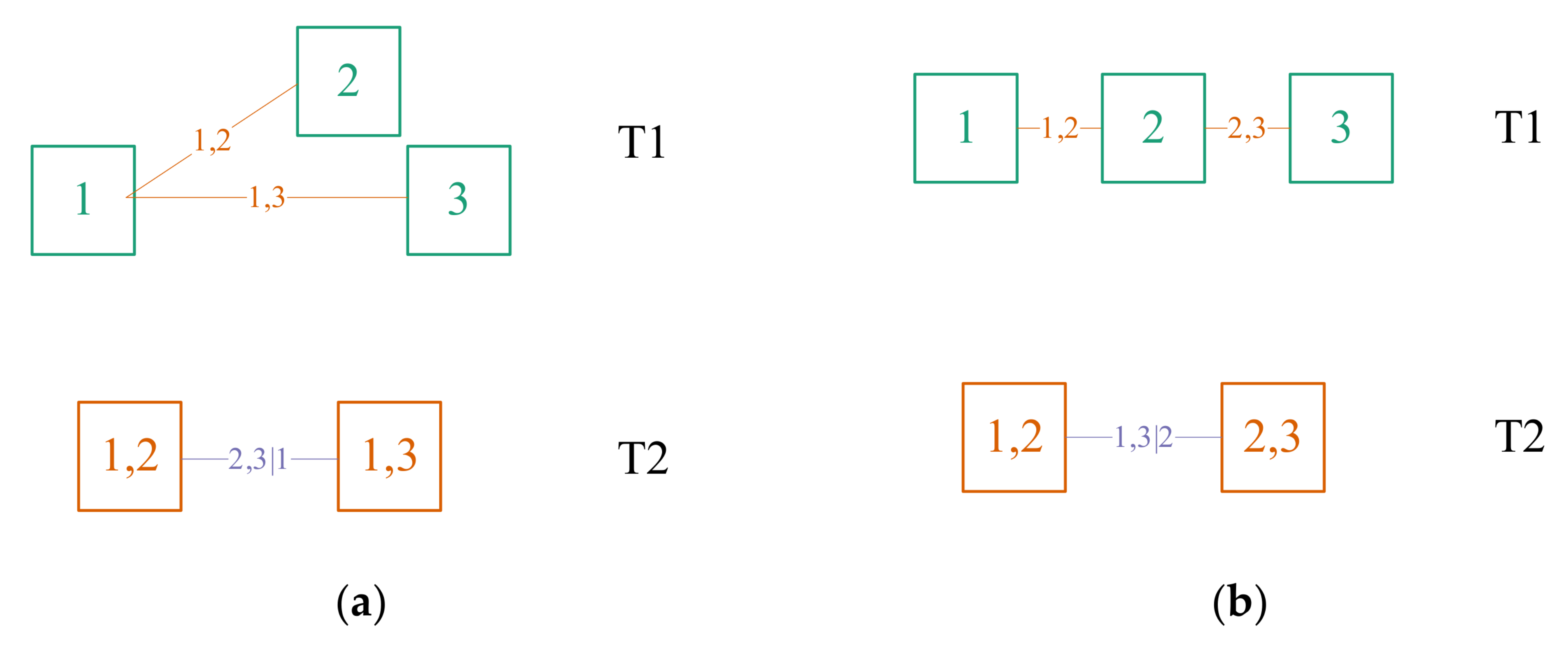
The vine copula function consists of a stack of conventional binary copula functions, which copulas marginal distributions or conditional marginal distributions [25], and their dependence structure can be graphically represented as vines. For example, two kinds of three-dimensional vine copula structures are shown in Figure 5. In vine copula structure, the vine consists of a series of trees, such as ‘T1’ and ‘T2’ in Figure 5a or Figure 5b; each tree consists of nodes (such as ‘1’ and ‘2’ in ‘T1’ in Figure 5a or Figure 5b, etc.) and edges (such as ‘1,2’ in ‘T1’ in Figure 5a or Figure 5b, etc.). Except the last tree, the edges of each tree are used as the nodes of the next tree. The nodes in the first tree represent the marginal distributions of each variable, such as ‘1’ represents $F_1(x_1)$; the edges in the first tree represent the binary joint distributions of the two nodes linked, such as ‘1,2’ represents $C_{1,2}[F_1(x_1),F_2(x_2)]$; the edges in other trees represent the binary conditional joint distributions of the two nodes linked, such as ‘1,3|2’ represents $C_{1,3|2}[F_{1|2}(x_1|x_2),F_{3|2}(x_3|x_2)]$.

The three-dimensional vine copula function has two kinds of structures: the canonical vine copula and the D-vine copula. In canonical vine copula structure, there is one central node in each tree that is linked to all edges, as shown in Figure 5a; in D-vine copula structure, each node is linked to at most two edges, as shown in Figure 5b. When using the canonical vine copula structure, not only the central node of the first tree but also the central node of each subsequent tree needs to be determined; when using the D-vine copula structure, since all the trees are in the form of chains, once the order of the nodes of the first tree is determined, the subsequent trees are also determined.

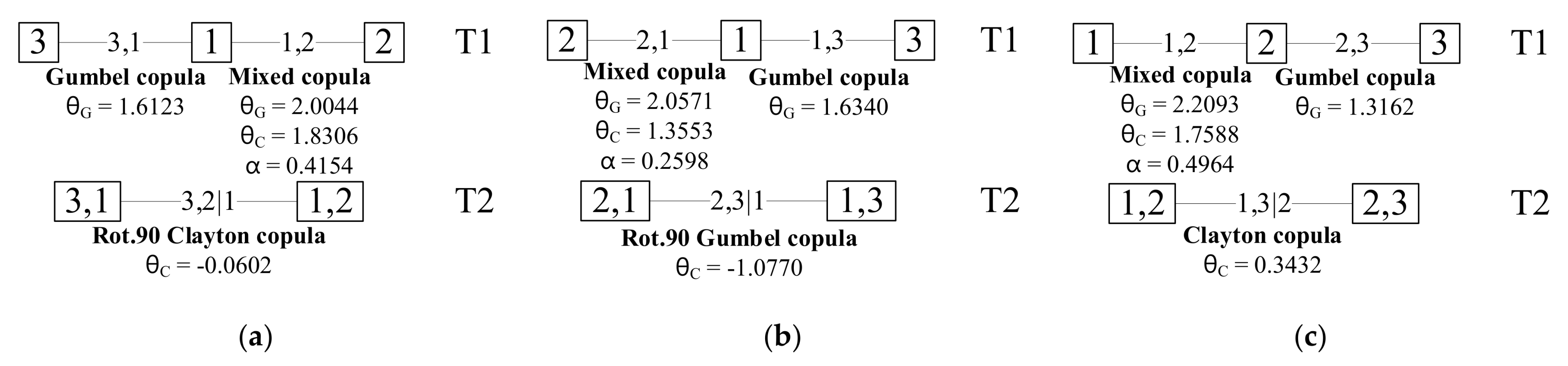
When choosing copula functions, different copula functions have different characteristics and applicability conditions. Gumbel copula is suitable for portraying random variables with upper-tail correlation, such as design flood; Clayton copula is suitable for portraying random variables with lower-tail correlation, such as dry-season runoff. Considering that it is often difficult for a single copula function to accurately capture the correlation structure among variables, a mixed copula function of Gumbel copula and Clayton copula is constructed in this paper, as follows:

$$C_{mix}(u_1,u_2;\alpha ,{\theta }_G,{\theta }_C)=\alpha C_G(u_1,u_2;{\theta }_G)+(1-\alpha )C_C(u_1,u_2;{\theta }_C)$$

(2)

where $\alpha$ is the ratio of $C_G$ in the mixed copula; $C_G$ is Gumbel copula, ${\theta }_G$ is the parameter of Gumbel copula; $C_C$ is Clayton copula, ${\theta }_C$ is the parameter of Clayton copula; $C_{mix}$ is the mixed copula.

The binary Gumbel copula and Clayton copula can only be applied in the case of a positive correlation between two variables. In this paper, when the case of negative correlation is encountered, the copula function is rotated by 90 degrees and the transformation relationship is as follows:

$$C_{R90}(u_1,u_2;\theta )=u_2-C(1-u_1,u_2;-\theta )$$

(3)

where $C_{R90}$ is the copula function after 90° rotation (Rot.90 copula); $\theta$ is the parameter of copula after 90° rotation. Like the original copula function, the rotated copula function can construct the mixed copula function and be used as the basis for the construction of the vine copula function.

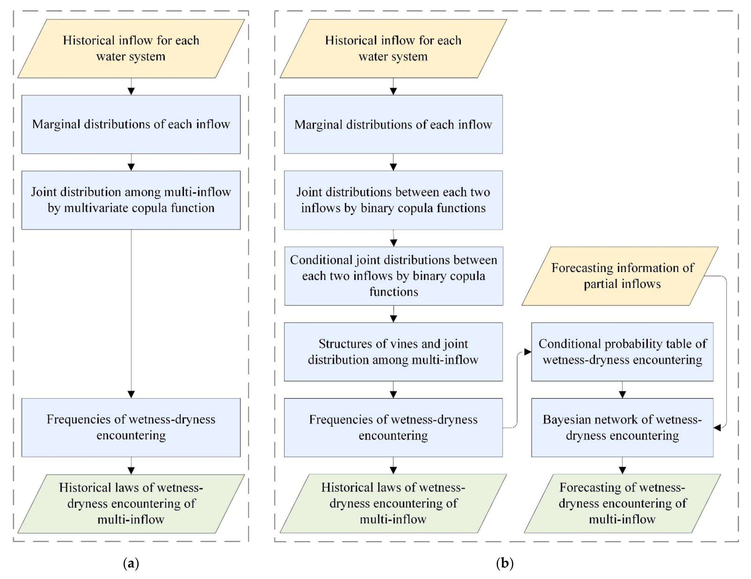
The flowchart of construction of the joint distribution by vine copula function can be found in Figure 3b, and the specific steps are as follows:

• Fitting of the marginal distributions of each inflow.

Fitting of the marginal distribution of each inflow means the determination of the nodes in the first tree in the vine copula function. The maximum likelihood method is used for parameter estimation among the commonly used distribution models in hydrology [38,39], and then the fitting test is performed using Kolmogorov–Smirnov(K-S) test. Among the tested distribution models, the appropriate distribution model is selected according to goodness-of-fit evaluation indexes such as RMSE value and AIC value, and the marginal distribution of each inflow is determined.

2.

Construction of the joint distributions between each two inflows.

Here to determine edges in the first tree. The inflow series is introduced into the respective marginal distribution to obtain the marginal CDF value series. Kendall’s tau coefficient ($\tau$ value) of each two inflows is calculated from the marginal CDF value series. If $\tau >0$, the two variables are positively correlated, the parameter estimation is performed for the binary Gumbel copula and Clayton copula; if $\tau <0$, the two variables are negatively correlated, the parameter estimation is performed for the binary Gumbel copula rotated 90° and Clayton copula rotated 90°. The maximum likelihood method is employed for parameter estimation, and the nonlinear programming method was used to obtain the α value of the mixed copula, taking the RMSE value minimum as the objective function. Then the fitting test is performed, and among the copula functions that pass the test, the appropriate copula function is selected based on the results of the goodness-of-fit evaluation.

3.

Construction of the conditional joint distributions between each two inflows.

Here, we determine the edges of trees except the first tree. From the edges of the previous one tree, the conditional marginal distributions of each inflow are derived. The inflow series or the marginal CDF value series obtained in the previous step is introduced into the respective conditional marginal distribution, in order to obtain the conditional marginal CDF value series. The conditional joint distributions between each two inflows are constructed from the conditional marginal CDF value series by the binary copula function, and the method is the same as that in step 2. The derivation of the conditional marginal distributions of each inflow from edges in the first tree can be expressed in the following two general equations:

$$F_{i|j}(x_i|x_j)=\frac{\partial C_{i,j}[F_i(x_i),F_j(x_j)]}{\partial F_j(x_j)}$$

(4)

or

$$F_{i|j}(x_i|x_j)=\frac{\partial C_{j,i}[F_j(x_j),F_i(x_i)]}{\partial F_j(x_j)}$$

(5)

The derivation of the conditional marginal distributions of each inflow from edges in other trees can be expressed in the following two general equations:

$$F_{i|\overrightarrow{v}}(x_i|\overrightarrow{v})=\frac{\partial C_{i,j|{\overrightarrow{v}}_{-j}}[F_{i|{\overrightarrow{v}}_{-j}}(x_i|{\overrightarrow{v}}_{-j}),F_{j|{\overrightarrow{v}}_{-j}}(x_j|{\overrightarrow{v}}_{-j})]}{\partial F_{j|{\overrightarrow{v}}_{-j}}(x_j|{\overrightarrow{v}}_{-j})}$$

(6)

or

$$F_{i|\overrightarrow{v}}(x_i|\overrightarrow{v})=\frac{\partial C_{j,i|{\overrightarrow{v}}_{-j}}[F_{j|{\overrightarrow{v}}_{-j}}(x_j|{\overrightarrow{v}}_{-j}),F_{i|{\overrightarrow{v}}_{-j}}(x_i|{\overrightarrow{v}}_{-j})]}{\partial F_{j|{\overrightarrow{v}}_{-j}}(x_j|{\overrightarrow{v}}_{-j})}$$

(7)

where $\overrightarrow{v}$ is an n-dimensional vector, $x_j$ is any variable in $\overrightarrow{v}$, and ${\overrightarrow{v}}_{-j}$ is the vector composed of the remaining (n-1) variables.

4.

Selection of vine copula structures and derivation of joint distributions among multi-inflow.

Vine copula structures are flexible and numerous, and even for a canonical vine copula or D-vine copula, there are in total d! structures on d inflows [40]. The vine structures can be determined by the sequential maximum spanning tree optimization method [26]. This method looks for the tree with the maximal sum of weights under the assumption that the higher the sum of weights, the better the goodness-of-fit [41]. Since the weights of trees represent the goodnesses-of-fit, the opposites of the AIC values are chosen as weights, i.e.,

$$\max [{\displaystyle \sum _{T=1}^{d-1}{\displaystyle \sum _{N=1}^{d-T}(-AI{C}_{N,T}}})]$$

(8)

where T is the index of trees in the vine copula functions, and N is the index of edges in the trees.

The derivation of joint distributions among multi-inflow from vine copula structures can be expressed in the following equation:

$$\begin{array}{l}{F}_{1,2,\cdots ,d}(x_1,x_2,\cdots ,x_d)=C_{1,2,\cdots ,d}[F_1(x_1),F_2(x_2),\cdots ,F_d(x_d)]\\ ={\displaystyle {\int }_0^{F({\overrightarrow{v}}_{-j,-k}(1))}\cdots {\displaystyle {\int }_0^{F({\overrightarrow{v}}_{-j,-k}(d-2))}{C}_{j,k|{\overrightarrow{v}}_{-j,-k}}[F_{j|{\overrightarrow{v}}_{-j,-k}}(x_j|{\overrightarrow{v}}_{-j,-k}),F_{k|{\overrightarrow{v}}_{-j,-k}}(x_k|{\overrightarrow{v}}_{-j,-k})]d{\overrightarrow{v}}_{-j,-k}(1)\cdots d{\overrightarrow{v}}_{-j,-k}(d-2)}}\end{array}$$

(9)

where ${\overrightarrow{v}}_{-j,-k}(i)$ represents the i-th variable (i = 1, 2, …, d − 2) in ${\overrightarrow{v}}_{-j,-k}$. The joint distribution of the three variables as shown in Figure 5a can be expressed in the following equation:

$$F_{1,2,3}(x_1,x_2,x_3)=C_{1,2,3}[F_1(x_1),F_2(x_2),F_3(x_3)]={\displaystyle {\int }_0^{F_1(x_1)}{C}_{2,3|1}[F_{2|1}(x_2|x_1),F_{3|1}(x_3|x_1)]d{F}_1(x_1)}$$

(10)

3.2.2. Calculation for the Historical Statistical Probability of Wetness-Dryness Encountering

The historical statistical probability of wetness-dryness encountering is calculated by the joint distribution established in Section 3.2.1. According to the principle of probabilistic mutual exclusion, the probability of wetness-dryness encountering of d water systems can be calculated by the following equation:

$$P(a_{1,1}\le u_1<a_{2,1},a_{1,2}\le u_2<a_{2,2},\cdots ,a_{1,d}\le u_d<a_{2,d})={\displaystyle \sum _{i_1=1}^2{\displaystyle \sum _{i_2=1}^2\cdots {\displaystyle \sum _{i_d=1}^2{(-1)}^{i_1+i_2+\cdots +i_d}C(a_{i_1,1},a_{i_2,2},\cdots ,a_{i_d,d})}}}$$

(11)

For example, the equation for calculating the probability of wetness-dryness encountering of 3 water systems is:

$$\begin{array}{l}P(a_{1,1}\le u_1<a_{2,1},a_{1,2}\le u_2<a_{2,2},a_{1,3}\le u_3<a_{2,3})\\ =-C(a_{1,1},a_{1,2},a_{1,3})+C(a_{1,1},a_{1,2},a_{2,3})+C(a_{1,1},a_{2,2},a_{1,3})-C(a_{1,1},a_{2,2},a_{2,3})\\ \hspace{1em}+C(a_{2,1},a_{1,2},a_{1,3})-C(a_{2,1},a_{1,2},a_{2,3})-C(a_{2,1},a_{2,2},a_{1,3})+C(a_{2,1},a_{2,2},a_{2,3})\end{array}$$

(12)

where $C( )$ is the joint distribution derived by Equation (9).

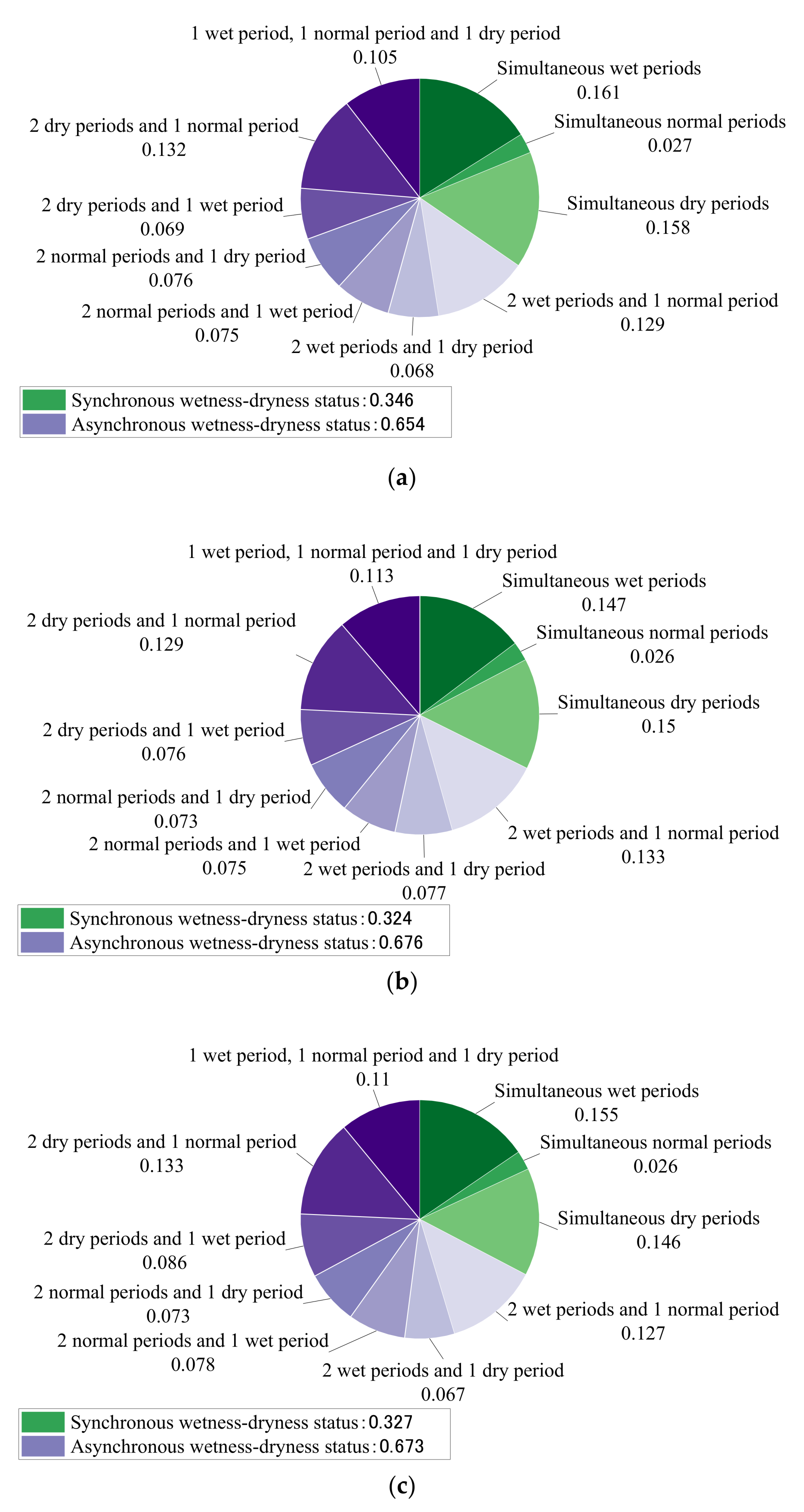
3.2.3. Forecasting for the Probability of Wetness-Dryness Encountering

The probability of wetness-dryness encountering is forecast from the historical statistical probability of wetness-dryness encountering in addition to forecasting information of some water systems by Bayesian networks. Based on the conditional probability formula and Bayes’ theorem, Bayesian networks [29] are directed acyclic graphs with a mesh structure, which abstract random events into nodes of a network, and connect nodes with related relationships by directed arcs in order to graphically express the probabilities of random events as well as visualize the interactions between the elements. Bayes’ theorem was summarized by mathematician Bayes, in order to describe the relationship between conditional probabilities. Its main content is as follows: in a test, the sample space is S, A is the event of the test, and $B_1,B_2,\dots ,B_n$ is the division of the sample space S. Then, the probability is obtained as follows:

$$P(B_i|A)=\frac{P(A|B_i)P(B_i)}{{\displaystyle \sum _{j=1}^{n}P(A|B_j)P(B_j)}},i=1,2,\cdots ,n$$

(13)

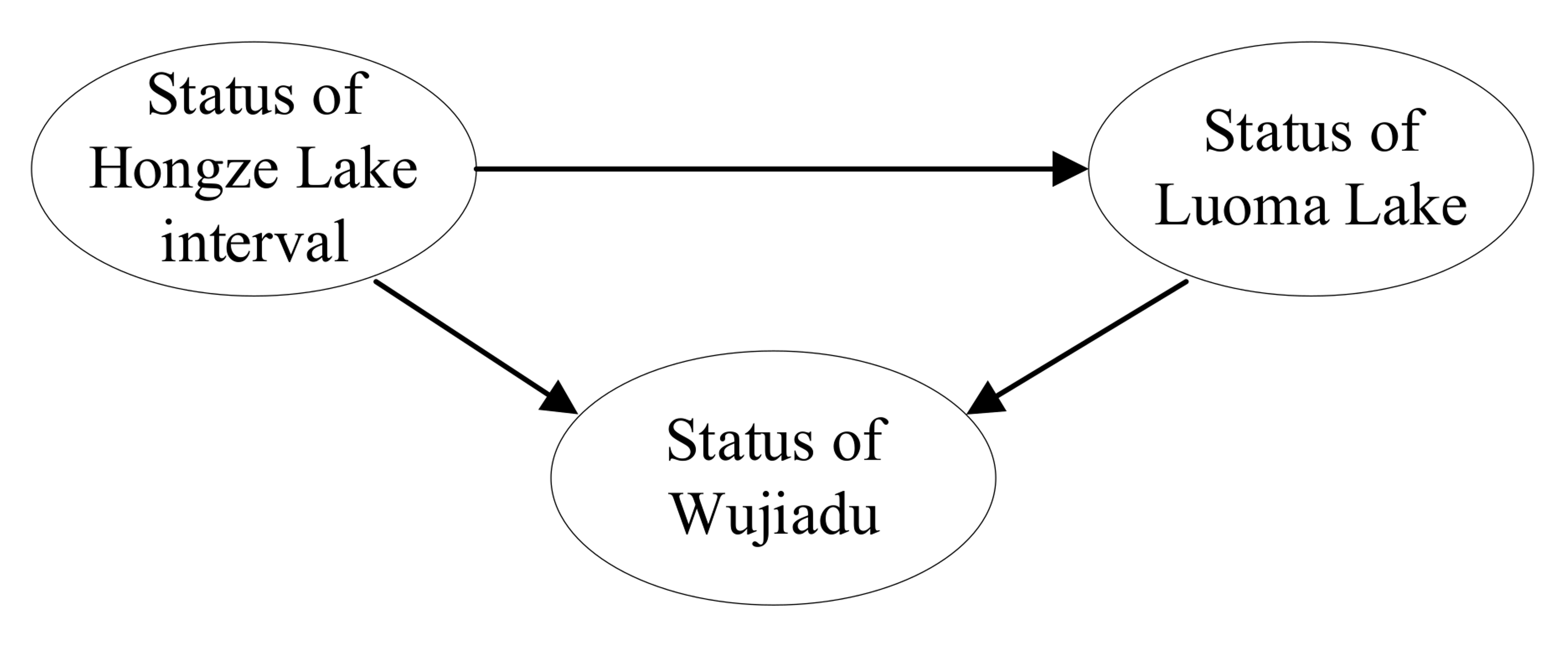
Bayesian networks consist of two parts: network structure and network parameters. The network structure refers to the topology established according to the causal relationship between nodes, which is generally expressed through a directed acyclic graph; the network parameters are the prior probability of the root nodes and the conditional probability of the non-root nodes, which are generally calculated according to the conditional probability table.

The main steps of forecasting for the probability of wetness-dryness encountering using Bayesian networks are as follows:

• Construction of a directed acyclic graph, i.e., the structure of the Bayesian network, based on the actual problem.
• Calculation for the conditional probability table. From the historical statistical probabilities of wetness-dryness encountering calculated in Section 3.2.2, the conditional probability table can be derived according to the conditional probability formula.
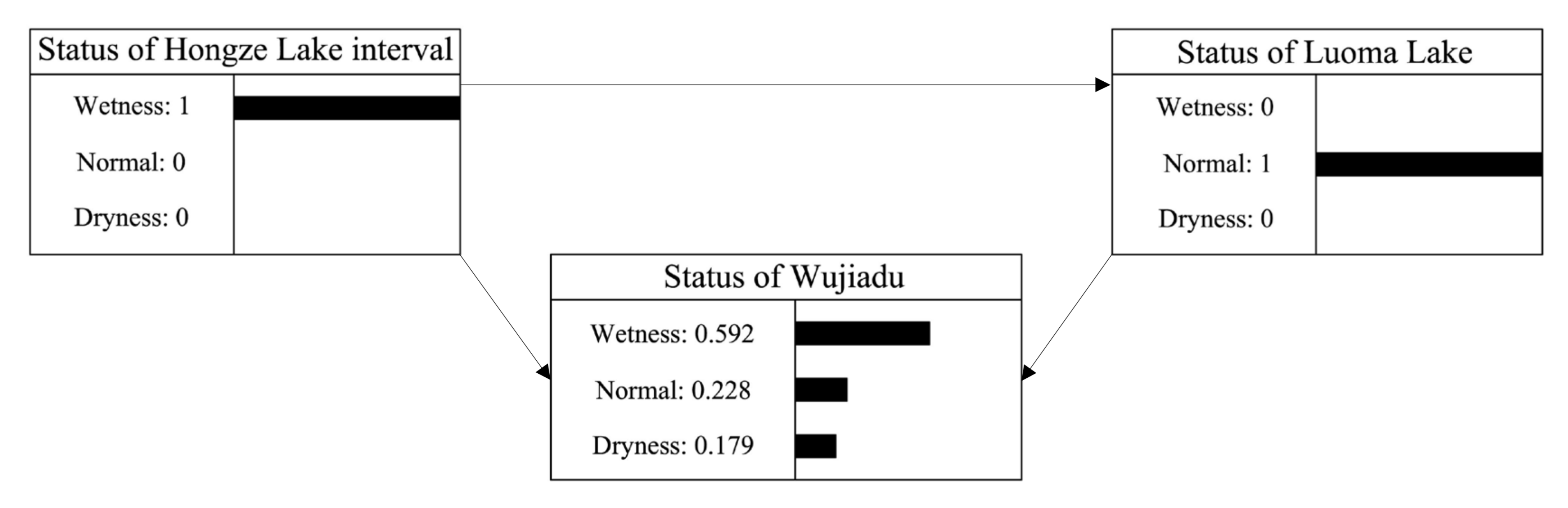
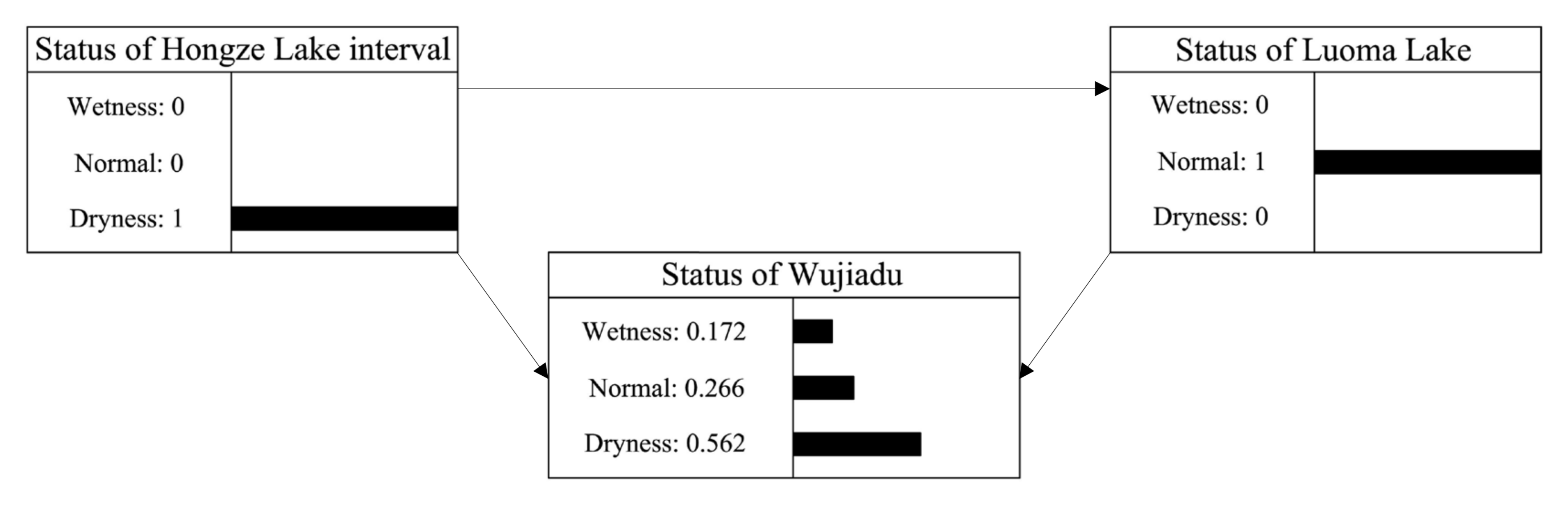
• Input forecasting information of some water systems into the Bayesian network, and the probability of wetness-dryness encountering in the future period can be obtained by the Bayesian network.

4. Results and Discussion

4.1. Construction of the Joint Distributions of Three Inflows

In this paper, we studied the wetness-dryness encountering of Wujiadu, Hongze Lake interval, and Luoma Lake at three scales: annual period, flood season, and non-flood season. Firstly, the joint distributions of inflows from three water systems at the three scales were constructed by the vine copula functions.

4.1.1. Fitting of Marginal Distributions of Each Inflow

The Weibull (WBL), normal (NORM), lognormal (LOGN), gamma (GAM), and generalized extreme value (GEV) distributions were selected as alternatives for representing the marginal distribution of inflow. The maximum likelihood method was used to fit marginal distributions of inflow of Hongze Lake interval, Wujiadu, and Luoma Lake at three scales: annual period, flood season, and non-flood season. The K-S tests were used for the fitting test, and the significance level was 0.05. The test results are shown in

Table 1. Fitting test for marginal distributions of each inflow.

Scale	Inflows	D0.05	D
			WBL	NORM	LOGN	GAM	GEV
Annual period	Hongze Lake interval	0.174	0.061	0.131	0.064	0.045	0.048
	Wujiadu	0.174	0.067	0.092	0.108	0.071	0.074
	Luoma Lake	0.174	0.089	0.173	0.061	0.077	0.053
Flood season	Hongze Lake interval	0.174	0.062	0.159	0.081	0.055	0.069
	Wujiadu	0.174	0.056	0.081	0.105	0.067	0.074
	Luoma Lake	0.174	0.061	0.162	0.085	0.054	0.066
Non-flood season	Hongze Lake interval	0.176	0.063	0.139	0.135	0.076	0.071
	Wujiadu	0.176	0.098	0.155	0.055	0.084	0.066
	Luoma Lake	0.176	0.089	0.188 *	0.055	0.088	0.052

* The D value in the table is displayed in bold font if the hypothesis test at the significance level of 0.05 is not passed.

.

As shown in Table 1, the hypothesis of normal distribution was rejected for the inflow of Luoma Lake in non-flood season at the significance level of 0.05, while the hypotheses of the other four distributions were accepted; the hypotheses of the above five distributions were accepted for other inflows or other scales. The rejection of the hypothesis of normal distribution for the inflow of Luoma Lake in non-flood season has a 5% probability of being caused by a type I error of the hypothesis test. If the significance level is set to 0.01 in order to further control the probability of a type I error, the critical value would be 0.210, and the inflow of Luoma Lake in non-flood season would accept the hypothesis of normal distribution. The AIC values of each marginal distribution model are shown in

Table 2. The AIC values of each marginal distribution.

Scale	Inflows	AIC
		WBL	NORM	LOGN	GAM	GEV
Annual period	Hongze Lake interval	−453.2	−310.9	−420.3	−481.0 *	−455.0
	Wujiadu	−420.7	−385.6	−365.0	−396.8	−385.7
	Luoma Lake	−427.6	−303.7	−432.4	−448.3	−452.8
Flood season	Hongze Lake interval	−422.1	−281.1	−431.5	−430.0	−434.5
	Wujiadu	−453.9	−368.6	−345.5	−421.3	−421.5
	Luoma Lake	−438.6	−298.4	−396.3	−450.2	−445.2
Non-flood season	Hongze Lake interval	−437.1	−311.9	−332.5	−422.1	−418.4
	Wujiadu	−367.3	−302.0	−436.9	−389.4	−424.3
	Luoma Lake	−375.0	−263.7	−463.1	−382.5	−475.2

* The lowest AIC value is displayed in bold font.

.

The appropriate distribution models at each scale were selected according to the AIC values, and marginal distribution scheme I was obtained and shown in

Table 3. Scheme I of the marginal distributions and their distribution parameters.

Scale	Inflows	Marginal Distribution	Distribution Parameters
			Parameter 1	Parameter 2	Parameter 3
Annual period	Hongze Lake interval	GAM	a = 1.8650	b = 70.9392	——
	Wujiadu	WBL	a = 909.5822	b = 1.8870	——
	Luoma Lake	GEV	k = 0.2799	σ = 69.2419	μ = 93.3307
Flood season	Hongze Lake interval	GEV	k = 0.4068	σ = 132.2953	μ = 160.6528
	Wujiadu	WBL	a = 1603.5	b = 1.4398	——
	Luoma Lake	GAM	a = 1.4378	b = 239.7519	——
Non-flood season	Hongze Lake interval	WBL	a = 48.4864	b = 1.2029	——
	Wujiadu	LOGN	μ = 5.9707	σ = 0.6480	——
	Luoma Lake	GEV	k = 0.4084	σ = 25.6053	μ = 31.9731

. In this scheme, the GAM, WBL, and GEV distributions were chosen, respectively, to fit the inflows from Hongze Lake interval, Wujiadu, and Luoma Lake under the annual scale; in flood season, the GEV, WBL, and GAM distributions were chosen, respectively, to fit the inflows from the above three water systems; in non-flood season, the WBL, LOGN and GEV distributions were chosen, respectively, to fit the inflows from the above three water systems.

In practical application, the climates of the three water systems are close to each other; thus, the statistical characteristics of the inflows should be basically similar, and it is possible to fit the marginal distributions using uniform distribution models. In this paper, the differences within 10% of the AIC value were ignored, and the uniform distribution models at each scale were recommended by analyzing the results in Table 2 comprehensively.

Under the annual scale, the difference between the AIC values of Wujiadu inflow fitted by the GAM and WBL distribution is only 5.68%; the difference between the AIC values of Luoma Lake inflow fitted by the GAM and GEV distribution is only 0.99%. Therefore, the marginal distributions of the inflows under the annual scale were recommended to be fitted by the GAM distribution.

In flood season, the difference between the AIC values of Hongze Lake interval inflow fitted by the GAM and GEV distribution is only 1.04%; the difference between the AIC values of Wujiadu inflow fitted by the GAM and WBL distribution is only 7.18%. Therefore, the marginal distributions of the inflows in flood season were recommended to be fitted by the GAM distribution.

In non-flood season, the difference between the AIC values of Hongze Lake interval inflow fitted by the GEV and WBL distribution is only 4.28%; the difference between the AIC values of Wujiadu inflow fitted by the GEV and LOGN distribution is only 2.89%. Therefore, the marginal distributions of the inflows in non-flood season were recommended to be fitted by the GEV distribution.

Thus, the uniform distribution models at each scale were recommended, and marginal distribution scheme II was obtained and shown in

Table 4. Scheme II of the marginal distributions and their distribution parameters.

Scale	Marginal Distribution	Inflows	Distribution Parameters
			Parameter 1	Parameter 2	Parameter 3
Annual period	GAM	Hongze Lake interval	a = 1.8650	b = 70.9392	——
		Wujiadu	a = 2.9194	b = 275.7250	——
		Luoma Lake	a = 1.8072	b = 86.2970	——
Flood season	GAM	Hongze Lake interval	a = 1.4527	b = 210.2675	——
		Wujiadu	a = 1.6994	b = 858.8112	——
		Luoma Lake	a = 1.4378	b = 239.7519	——
Non-flood season	GEV	Hongze Lake interval	k = 0.2299	σ = 23.0285	μ = 26.4709
		Wujiadu	k = 0.2068	σ = 190.7822	μ = 322.3065
		Luoma Lake	k = 0.4084	σ = 25.6053	μ = 31.9731

.

In the following parts of Section 4.1, Section 4.2, Section 4.3 and Section 4.4, we discuss the results based on scheme I. The comparison of results based on scheme I and scheme II are further analyzed in Section 4.5.

4.1.2. Construction of the Joint Distributions between Each Two Inflows

The inflow series from the three water systems at three scales was introduced into the respective marginal distribution (scheme I) obtained in Section 4.1.1, and their respective marginal CDF value series were obtained. The joint distributions between each two inflows, i.e., the edges in the first tree in the vine copula structure at three scales, were fitted using the maximum likelihood method by the marginal CDF value series. The K-S tests were used for the fitting test, and the significance level was 0.05. The results of the parameter estimation and K-S tests of the binary copula functions between each two inflows are shown in

Table 5. The results of the parameter estimation and K-S tests of the binary copula functions between each two inflows.

Scale	Combination of Inflows	τ	Parameters			D0.05	D
			θG	θC	α		Gumbel	Clayton	Mixed
Annual period	1,2 and 2,1	0.579	2.0044	1.8306	0.4154	0.174	0.110	0.095	0.101
	1,3 and 3,1	0.442	1.6123	0.8325	1	0.174	0.086	0.124	0.086
	2,3 and 3,2	0.250	1.3083	0.3656	0.7302	0.174	0.091	0.100	0.093
Flood season	1,2 and 2,1	0.548	2.0571	1.3553	0.2598	0.174	0.062	0.053	0.053
	1,3 and 3,1	0.412	1.6340	0.8233	1	0.174	0.068	0.109	0.068
	2,3 and 3,2	0.228	1.2300	0.1982	1	0.174	0.082	0.099	0.082
Non-flood season	1,2 and 2,1	0.534	2.2093	1.7588	0.4964	0.176	0.052	0.072	0.059
	1,3 and 3,1	0.287	1.3452	0.4582	1	0.176	0.056	0.070	0.056
	2,3 and 3,2	0.228	1.3162	0.3783	0.8860	0.176	0.050	0.055	0.046

. In the following figures and tables, ‘1’, ‘2’, and ‘3’ represent Hongze Lake interval, Wujiadu, and Luoma Lake inflow, respectively; ‘i, j’ represents $C_{i,j}(u_i,u_j)$; i = 1, 2, 3; j = 1, 2, 3; i ≠ j.

According to the results of the K-S tests, all copula functions that were fitted passed the hypothesis test with a significance level of 0.05. The copula functions were selected according to the AIC values. The AIC values and selected copulas are shown in

Table 6. The AIC values and selected copula functions between each two inflows.

Scale	Combination of Inflows	AIC			Selected Copula
		Gumbel	Clayton	Mixed
Annual period	1,2 and 2,1	−411.2	−416.4	−418.1 *	Mixed
	1,3 and 3,1	−426.6	−385.5	−422.6	Gumbel
	2,3 and 3,2	−414.5	−408.1	−411.6	Gumbel
Flood season	1,2 and 2,1	−423.8	−455.2	−457.2	Mixed
	1,3 and 3,1	−432.8	−404.4	−428.8	Gumbel
	2,3 and 3,2	−407.1	−384.8	−403.1	Gumbel
Non-flood season	1,2 and 2,1	−440.3	−440.8	−452.8	Mixed
	1,3 and 3,1	−438.1	−415.4	−434.1	Gumbel
	2,3 and 3,2	−470.2	−446.7	−466.7	Gumbel

* The lowest AIC value is displayed in bold font.

.

4.1.3. Construction of the Conditional Joint Distributions between Each Two Inflows

The inflow series or the marginal CDF value series from three water systems at three scales were introduced into the respective conditional marginal distribution, which can be obtained by Equations (4) and (5), in addition to the joint distributions between each two inflows constructed in Section 4.1.2.; then, their respective conditional marginal CDF value series was obtained. The conditional joint distributions between each two inflows, i.e., the edges in the second tree in the vine copula structure at three scales were fitted using the conditional marginal CDF value series. The methods for fitting, fitting tests, and copula function selection were the same as those used in Section 4.1.2. The results of the parameter estimation and K-S tests of the conditional binary copula functions between each two inflows are shown in

Table 7. The results of the parameter estimation and K-S tests of the conditional binary copula functions between each two inflows.

Scale	Combination of Inflows	τ	Parameters			D0.05	D
			θG	θC	α		Gumbel	Clayton	Mixed
Annual period	1,3|2 and 3,1|2	0.339	1.4634	0.8494	0.1306	0.174	0.092	0.075	0.076
	1,2|3 and 2,1|3	0.544	1.8043	1.7053	0	0.174	0.132	0.127	0.127
	2,3|1	−0.113	−1.0897	−0.3555	1	0.174	0.069	0.083	0.069
	3,2|1	−0.113	−1.1592	−0.0602	0.0473	0.174	0.080	0.067	0.067
Flood season	1,3|2 and 3,1|2	0.534	1.6116	0.9246	0.3355	0.174	0.075	0.067	0.067
	1,2|3 and 2,1|3	0.372	1.9346	1.3821	0.0930	0.174	0.112	0.089	0.087
	2,3|1	−0.174	−1.0770	−0.4710	0.7522	0.174	0.066	0.089	0.071
	3,2|1	−0.174	−1.1969	−0.0938	0.4739	0.174	0.082	0.063	0.072
Non-flood season	1,3|2 and 3,1|2	0.119	1.1442	0.3432	0	0.176	0.093	0.085	0.085
	1,2|3 and 2,1|3	0.528	1.9706	1.6772	0.4632	0.176	0.069	0.087	0.070
	2,3|1 and 3,2|1	0.068	1.0464	0.1059	0	0.176	0.084	0.085	0.085

. In the following figures and tables, ‘i, j| k’ represents $C_{i,j|k}[F_{i|k}(x_i|x_k),F_{j|k}(x_j|x_k)]$; i = 1, 2, 3; j = 1, 2, 3; i ≠ j.

According to the results of the K-S tests, all copula functions that were fitted passed the hypothesis test with a significance level of 0.05. Similarly, the copula functions were selected according to the AIC values. The AIC values and selected conditional copulas are shown in

Table 8. The AIC values and selected conditional copula functions between each two inflows.

Scale	Combination of Inflows	AIC			Selected Copula
		Gumbel	Clayton	Mixed
Annual period	1,3|2 and 3,1|2	−411.2	−425.2 *	−421.5	Clayton
	1,2|3 and 2,1|3	−364.0	−390.7	−386.7	Clayton
	2,3|1	−452.1	−426.7	−448.1	Rot.90 Gumbel
	3,2|1	−433.4	−454.1	−450.2	Rot.90 Clayton
Flood season	1,3|2 and 3,1|2	−416.7	−427.3	−427.3	Clayton
	1,2|3 and 2,1|3	−377.2	−395.3	−391.5	Clayton
	2,3|1	−440.9	−426.8	−438.8	Rot.90 Gumbel
	3,2|1	−435.0	−436.4	−438.4	Mixed
Non-flood season	1,3|2 and 3,1|2	−407.1	−425.1	−421.1	Clayton
	1,2|3 and 2,1|3	−418.9	−421.5	−425.6	Mixed
	2,3|1 and 3,2|1	−411.4	−416.0	−412.0	Clayton

* The lowest AIC value is displayed in bold font.

.

4.1.4. Selection of Vine Copula Structures and Derivation of Joint Distributions among Multi-Inflows

In this paper, the three water systems were on equal footing, thus the D-vine structure was selected. The opposites of the AIC values were used as the weights, thus the sum of the weight of each D-vine structure was calculated and shown in

Table 9. The sum of the weight of each D-vine structure.

Scale	The First Tree of the D-Vine Structure
	1-2-3 and 3-2-1	1-3-2 and 2-3-1	2-1-3	3-1-2
Annual period	1257.7	1231.8	1296.8	1298.8 *
Flood season	1291.6	1235.2	1330.9	1328.4
Non-flood season	1348.1	1333.9	1306.8	1306.8

* The highest value is displayed in bold font.

. The vine structure with the highest weight sum in each scale was selected and shown in Figure 6.

The joint distributions among three inflows at three scales were derived by Equation (9) according to the selected vine structures. Under the annual scale, the joint distribution among three inflows can be expressed as:

$$\begin{array}{l}{F}_{annual}(x_1,x_2,x_3)=C_{annual}(u_1,u_2,u_3)\\ ={\displaystyle {\int }_0^{u_1}{C}_{C,R90}[\frac{\partial C_G(u_3,u_1;1.6123)}{\partial u_1},\frac{\partial C_{mix}(u_1,u_2;0.4154,2.0044,1.8306)}{\partial u_1};-0.0602]d{u}_1}\end{array}$$

(14)

where $C_{C,R90}$ is Rot.90 Clayton copula. In flood season, the joint distribution among three inflows can be expressed as:

$$\begin{array}{l}{F}_{flood}(x_1,x_2,x_3)=C_{flood}(u_1,u_2,u_3)\\ ={\displaystyle {\int }_0^{u_1}{C}_{G,R90}[\frac{\partial C_{mix}(u_2,u_1;0.2598,2.0571,1.3553)}{\partial u_1},\frac{\partial C_G(u_1,u_3;1.6340)}{\partial u_1};-1.0770]d{u}_1}\end{array}$$

(15)

where $C_{G,R90}$ is Rot.90 Gumbel copula. In non-flood season, the joint distribution among three inflows can be expressed as:

$$\begin{array}{l}{F}_{non-flood}(x_1,x_2,x_3)=C_{non-flood}(u_1,u_2,u_3)\\ ={\displaystyle {\int }_0^{u_2}{C}_C[\frac{\partial C_{mix}(u_1,u_2;0.4964,2.2093,1.7588)}{\partial u_2},\frac{\partial C_G(u_2,u_3;1.3162)}{\partial u_2};0.3432]d{u}_2}\end{array}$$

(16)

The function images of the joint distributions among three inflows at three scales are drawn, as shown in Figure 7.

4.2. The Analysis of Wetness-Dryness Encountering of Three Water Systems

The statuses at three scales of Hongze Lake interval, Wujiadu, and Luoma Lake were divided into wetness, normal, and dryness, according to the division criteria in Section 3.1. The frequencies of the 27 kinds of wetness-dryness encountering at three scales were calculated by the joint distributions constructed in Section 4.1. At the same time, the observed values of the frequencies of each wetness-dryness encountering were obtained by counting the historical data. The observed and calculated values of frequencies of wetness-dryness encountering are shown in Figure 8, which show that the observed and calculated values of frequencies did not differ by much. As a result of the limited length of historical data, some of the observed values of the frequencies of wetness-dryness encountering were 0. The calculated values seem to be more reasonable.

Further, the above 27 kinds of wetness-dryness encountering can be grouped into two major categories: synchronous wetness-dryness status and asynchronous wetness-dryness status. Synchronous wetness-dryness status includes three kinds of wetness-dryness encountering: simultaneous wet periods, simultaneous normal periods, and simultaneous dry periods. Asynchronous wetness-dryness status includes the other 24 kinds of wetness-dryness encountering, and can be categorized into seven kinds of combinations: two wet periods and one normal period, two wet periods and one dry period, two normal periods and one wet period, etc. There exist 10 kinds of combinations in total, and they are shown in Figure 9.

As shown in Figure 8 and Figure 9, the statistical laws of the wetness-dryness combinations at the three scales are basically the same. The frequencies of synchronous wetness-dryness status are all between 0.32 and 0.35, and the frequencies of asynchronous wetness-dryness status are all between 0.65 and 0.68, at the three scales. For each wetness-dryness combination, the frequency difference of different scales is within 0.025.

According to the definition of independence in the field of statistics, if the statuses of three water systems were independent of each other, the frequency of synchronous wetness-dryness status would be 0.121. In fact, the frequencies of the synchronous wetness-dryness statuses at three scales: annual period, flood season, and non-flood season are 0.346, 0.324, and 0.327, respectively. This shows that there is a correlation between the statuses of the three water systems. The reason for this is because the geographical locations of their catchment areas are close; the distance between each two representative hydrological stations are all within 150 km. Their catchments are all located in the monsoon climate area in eastern China, and the climate conditions and the underlying surface conditions are similar. Therefore, when the statuses of some water systems are wetness, normal, or dryness, there is a high probability that the statuses of other water systems are also wetness, normal, or dryness.

The existence of complementary statuses is the basis for the joint operation of a multi-water system. Here, the frequencies of the asynchronous wetness-dryness statuses at three scales are as follows: annual period, flood season, and non-flood season are 0.654, 0.676, and 0.673, respectively, which makes the joint operation of the three water systems feasible. For example, when the status of Wujiadu is wetness, and the statuses of Hongze Lake interval and Luoma Lake are dryness, the water supply from the main stream of Huaihe River can be increased, in order to reduce the water supply from six tributaries around Hongze Lake. At the same time, the water resources of the main stream of Huaihe River can be supplemented to Luoma Lake through Xuhonghe River. In this way, the amount of water transferred from the Yangtze River can be reduced, in order to reduce the water costs.

The non-flood season is the main period of water transfer from the Yangtze River. In non-flood season, when the three water systems are in the status of simultaneous dry periods, two dry periods and one normal period, or two normal periods and one dry period, local water resources may not be able to meet water demands. Under these situations, water transfer from the Yangtze River is necessary, and the sum of the frequencies of these situations is 0.351. It can be seen that the SNWTERP is of great significance in alleviating contradictions between supply and demand of water resources in this area.

4.3. The Forecasting of Wetness-Dryness Encountering of Three Water Systems

In this section, the forecasting of Wujiadu inflow and wetness-dryness encountering of three water systems when the status of Hongze Lake interval and Luoma Lake were obtained from 2017 to 2019 under the annual scale was conducted as an example. The Bayesian network structure was established and shown in Figure 10. The conditional probability table of wetness-dryness encountering was obtained by the conditional probability formula, and the historical statistical laws of wetness-dryness encountered in Section 4.2, and are shown in

Table 10. The conditional probability table of wetness-dryness encountering.

Status of Hongze Lake Interval	Luoma Lake		The Conditional Probability of Each Status of Wujiadu
	Status	Conditional Probability	Wetness	Normal	Dryness
Wetness	Wetness	0.663	0.645	0.201	0.153
	Normal	0.233	0.592	0.228	0.179
	Dryness	0.104	0.598	0.227	0.176
Normal	Wetness	0.350	0.308	0.316	0.376
	Normal	0.351	0.310	0.314	0.376
	Dryness	0.300	0.330	0.308	0.362
Dryness	Wetness	0.104	0.175	0.271	0.554
	Normal	0.200	0.172	0.266	0.562
	Dryness	0.697	0.157	0.239	0.604

.

The statuses of Hongze Lake interval and Luoma Lake from 2017 to 2019 were input into the Bayesian network as posterior information, in order to forecast the statuses of Wujiadu. In 2017 and 2018, the statuses of Hongze Lake interval and Luoma Lake were wetness and normal, respectively, and the Bayesian network diagram is shown in Figure 11; in 2019, the statuses of Hongze Lake interval and Luoma Lake were dryness and normal, respectively, and the Bayesian network diagram is shown in Figure 12.

As shown in Figure 11, the probability that the status of Wujiadu in 2017 and 2018 was wetness was the highest, which was 0.592. In this case, the wetness-dryness encountering of Hongze Lake interval, Wujiadu, and Luoma Lake was wetness-wetness-normal. As shown in Figure 12, the probability that the status of Wujiadu in 2019 was dryness was the highest, which was 0.562. In this case, the wetness-dryness encountering of Hongze Lake interval, Wujiadu, and Luoma Lake was dryness-dryness-normal. The statuses with the highest probability were selected as the forecasted results of the Bayesian network. The forecasted results and actual statuses from 2017 to 2019 are shown in

Table 11. The forecasted results and actual statuses from 2017 to 2019.

Year	Status of Wujiadu		Wetness-Dryness Encountering
	Forecasted	Actual	Forecasted	Actual
2017	W *	W	W-W-N	W-W-N
2018	W	W	W-W-N	W-W-N
2019	D	D	D-D-N	D-D-N

* In Table 11, W represents wetness, N represents normal, and D represents dryness.

.

As shown in Table 11, the actual status of Wujiadu in 2017 and 2018 was wetness, and the actual wetness-dryness encountering was wetness-wetness-normal; the actual status of Wujiadu in 2019 was dryness, and the actual wetness-dryness encountering was dryness-dryness-normal. The actual statuses were consistent with the forecasted results by the Bayesian network. It can be seen that the Bayesian network can effectively forecast the wetness-dryness encountering of multiple water systems by using the inflow information of some water systems, in order to provide support for the joint operation of multiple water systems.

4.4. Comparative Analysis of Vine Copula and Conventional Copula

In this paper, the joint distributions of inflows of Hongze Lake interval, Wujiadu, and Luoma Lake were also constructed by the conventional ternary copula functions, and the results were compared with those constructed by the vine copula functions. After construction by the conventional ternary copula functions, similarly, the fit tests were performed using the K-S method, and the copula functions were selected according to the AIC values. The results are shown in

Table 12. The results of the parameter estimation, K-S tests, AIC values, and selected copula functions of the ternary copula functions among three inflows.

Scale	Copula	θ	α	D0.05	D	AIC	Selected Copula
Annual period	Gumbel	1.5757		0.174	0.124	−377.5	Gumbel
	Clayton	0.8787		0.174	0.118	−360.0
	Mixed		0.8791	0.174	0.123	−373.8
Flood season	Gumbel	1.5563		0.174	0.104	−389.8	Gumbel
	Clayton	0.7225		0.174	0.130	−368.3
	Mixed		0.8483	0.174	0.104	−386.7
Non-flood season	Gumbel	1.4936		0.176	0.075	−404.7	Gumbel
	Clayton	0.6952		0.176	0.112	−386.6
	Mixed		0.7845	0.176	0.080	−402.4

.

As shown in Table 12, all copula functions that were fitted passed the hypothesis tests with a significance level of 0.05. Gumbel Copula was selected at all three scales. The RMSE values, R² values, and AIC values of results obtained by the conventional copula function and the vine copula function were calculated and compared, as shown in

Table 13. The RMSE values, R² values, and AIC values of results obtained by the conventional copula function and the vine copula function.

Period	Copula	RMSE	R2	AIC
Annual period	Vine copula	0.035	0.981	−399.5
	Conventional copula	0.045	0.969	−377.5
Flood season	Vine copula	0.033	0.982	−405.0
	Conventional copula	0.040	0.973	−389.8
Non-flood season	Vine copula	0.024	0.990	−439.2
	Conventional copula	0.034	0.980	−404.7

. The P-P plots of the observed values and calculated values by the conventional copula function and the vine copula function are shown in Figure 13.

As shown in Table 13, the RMSE values and AIC values of results obtained by the vine copula function were lower than those obtained by the conventional copula function, and the R² values were closer to 1 at all three scales. The above three indexes reflected that the fitting effect of the vine copula function on the joint distributions of multi-inflows was better than that of the conventional copula function. As shown in Figure 13, the calculated values obtained by the vine copula function were closer to the observed values than those obtained by the conventional copula function. It can be seen that the vine copula function can more accurately construct the multivariate joint distribution, and improve the accuracy of the calculation of the wetness-dryness encountering.

4.5. The Comparison of Results Based on Scheme I and Scheme II of Marginal Distributions Fitting

The joint distributions among three inflows were obtained based on scheme II of marginal distributions fitting. Under the annual period, the joint distribution among three inflows can be expressed as follows:

$$\begin{array}{l}{F}_{annual\prime }(x_1,x_2,x_3)=C_{annual\prime }(u_1,u_2,u_3)\\ ={\displaystyle {\int }_0^{u_1}{C}_{C,R90}[\frac{\partial C_G(u_3,u_1;1.6232)}{\partial u_1},\frac{\partial C_{mix}(u_1,u_2;0.4234,2.0331,1.7138)}{\partial u_1};-0.0002]d{u}_1}\end{array}$$

(17)

In flood season, the joint distribution among three inflows can be expressed as the following:

$$\begin{array}{l}{F}_{flood\prime }(x_1,x_2,x_3)=C_{flood\prime }(u_1,u_2,u_3)\\ ={\displaystyle {\int }_0^{u_1}{C}_{G,R90}[\frac{\partial C_{mix}(u_2,u_1;0.6642,1.9251,1.3569)}{\partial u_1},\frac{\partial C_G(u_1,u_3;1.6009)}{\partial u_1};-1.0911]d{u}_1}\end{array}$$

(18)

In non-flood season, the joint distribution among three inflows can be expressed as follows:

$$\begin{array}{l}{F}_{non–flood\prime }(x_1,x_2,x_3)=C_{non–flood\prime }(u_1,u_2,u_3)\\ ={\displaystyle {\int }_0^{u_2}{C}_C[\frac{\partial C_C(u_1,u_2;1.5500)}{\partial u_2},\frac{\partial C_G(u_2,u_3;1.3064)}{\partial u_2};0.2227]d{u}_2}\end{array}$$

(19)

The 27 kinds of wetness-dryness encountering at three scales were calculated by Equations (17)–(19), and the results are shown in Figure 14. As a contrast, the results based on scheme I are also shown in Figure 14.

As shown in Figure 14, the results of the two schemes were very close at all three scales. The average probability difference of the two schemes of 27 kinds of wetness-dryness encountering at three scales was only 0.0025, among which the probability difference of wetness-wetness-wetness combination in non-flood season was the largest, which was only 0.0217. Therefore, a uniform marginal distribution model can be used to fit the marginal distributions of inflows at each scale.

5. Conclusions

The joint operation of multiple water systems needs to be supported by the historical laws and forecasting information of wetness-dryness encountering for the multi-water system. The analysis of wetness-dryness encountering requires the construction of the joint distribution; the vine copula function improves the processing capability of the copula function for high-dimensional data, and is therefore suitable for the construction of multivariate joint distributions. The Bayesian network can make full use of the forecasting information of some water systems, in order to forecast wetness-dryness encountering. In this paper, we proposed an analysis and forecasting model based on a vine copula function-Bayesian network in order to analyze and forecast the wetness-dryness encountering of multiple water systems. We constructed the joint distributions of inflows of Hongze Lake interval, Wujiadu, and Luoma Lake, analyzed their wetness-dryness encountering in history, and forecast their wetness-dryness encountering from 2017 to 2019. The conclusions can be summarized as follows:

• The frequencies of the asynchronous wetness-dryness statuses at three scales all exceeded 0.65, which makes the joint operation of the three water systems feasible. In non-flood season, when the three water systems are in the status of simultaneous dry periods, two dry periods and one normal period, or two normal periods and one dry period, water transfer from the Yangtze River is necessary, and the probability of such a situation is 0.351. Thus, the SNWTERP is of great significance for alleviating contradictions between water supply and demand in the study area.
• The Bayesian network was established according to the historical statistical law of the three inflows. The inflow status of Hongze Lake interval and Luoma Lake in 2017–2019 under the annual scale were input into the Bayesian network as posterior information, in order to forecast the wetness-dryness encountering of the three water systems in 2017–2019. The forecasting results are consistent with reality.
• The processing ability of the conventional copula function and the vine copula function for three-dimensional data was compared. The results show that the vine copula function can more accurately construct the multivariate joint distribution, and improve the accuracy of the calculation of the wetness-dryness encountering.
• The uniform distribution models can be used to fit the marginal distributions of inflows of Hongze Lake interval, Wujiadu, and Luoma Lake. Among them, the GEV distribution is recommended for the annual period and flood season; the GEV distribution is recommended for non-flood season.

References

1. Manshadi, H.R.D.; Niksokhan, M.H.; Ardestani, M. Water Allocation in Inter-Basin Water Transfer with the Virtual Water Approach. In Proceedings of the World Environmental and Water Resources Congress 2013: Showcasing the Future, Cincinnati, OH, USA, 19–23 May 2013. [Google Scholar]
2. Du, H.; Wang, Y.; Liu, K.; Cheng, L. Exceedance probability of precipitation for the Shuhe to Futuan Water Transfer Project in China. Environ. Earth Sci. 2019, 78, 240. [Google Scholar] [CrossRef]
3. Rosenberg, D.E.; Howitt, R.E.; Lund, J.R. Water management with water conservation, infrastructure expansions, and source variability in Jordan. Water Resour. Res. 2008, 44, W11402–W11411. [Google Scholar] [CrossRef]
4. Correia, F.N. Multivariate Partial Duration Series in Flood Risk Analysis. In Hydrologic Frequency Modeling; Springer: Dordrecht, The Netherlands, 1987; pp. 541–554. [Google Scholar]
5. Singh, K.; Singh, V.P. Derivation of bivariate probability density functions with exponential marginals. Stoch. Hydrol. Hydraul. 1991, 5, 55–68. [Google Scholar] [CrossRef]
6. Yue, S.; Ouarda, T.B.M.J.; Bobée, B.; Legendre, P.; Bruneau, P. The Gumbel mixed model for flood frequency analysis. J. Hydrol. 1999, 226, 88–100. [Google Scholar] [CrossRef]
7. Yue, S. The bivariate lognormal distribution to model a multivariate flood episode. Hydrol. Processes 2000, 14, 2575–2588. [Google Scholar] [CrossRef]
8. Liu, Z.; Guo, S.; Xu, X.; Xu, S.; Cheng, J. Application of Copula functions in hydrology and water resources: A state of the art review. Adv. Water Sci. 2021, 32, 148–159. [Google Scholar] [CrossRef]
9. Zening, W.; Chentao, H.; Wang, H.; Zhang, Q. Reservoir Inflow Synchronization Analysis for Four Reservoirs on a Mainstream and its Tributaries in Flood Season Based on a Multivariate Copula Model. Water Resour. Manag. 2020, 34, 2753–2770. [Google Scholar] [CrossRef]
10. Luo, Y.; Dong, Z.; Liu, Y.; Zhong, D.; Jiang, F.; Wang, X. Safety design for water-carrying Lake flood control based on copula function: A Case study of the Hongze Lake, China. J. Hydrol. 2021, 597, 126188. [Google Scholar] [CrossRef]
11. De Michele, C. A Generalized Pareto intensity-duration model of storm rainfall exploiting 2-Copulas. J. Geophys. Res. Atmos. 2003, 108, 4067. [Google Scholar] [CrossRef]
12. Kang, L.; He, X. Risk analysis of synchronous-asynchronous encounter probability of rich-poor precipitation in the middle route of South-to-North Water. Adv. Water Sci. 2011, 22, 44–50. [Google Scholar] [CrossRef]
13. Ahmadi, F.; Radmaneh, F.; Sharifi, M.R.; Mirabbasi, R. Bivariate frequency analysis of low flow using copula functions (case study: Dez River Basin, Iran). Environ. Earth Sci. 2018, 77, 643. [Google Scholar] [CrossRef]
14. Zellou, B.; Rahali, H. Assessment of the joint impact of extreme rainfall and storm surge on the risk of flooding in a coastal area. J. Hydrol. 2019, 569, 647–665. [Google Scholar] [CrossRef]
15. Wu, Y.; Zhong, P.; Wan, X.; Wang, H. Study on the Wetness-dryness Encountering of Inflow of Hanjiang-Rongjiang-Lianjiang Rivers Based on Copula Functions. Water Power 2021, 47, 10–15. [Google Scholar] [CrossRef]
16. Peng, Y.; Shi, Y.; Yan, H.; Chen, K.; Zhang, J. Coincidence Risk Analysis of Floods Using Multivariate Copulas: Case Study of Jinsha River and Min River, China. J. Hydrol. Eng. 2019, 24, 5018030. [Google Scholar] [CrossRef]
17. Zhao, R.; Wang, H.; Hu, S.; Zhan, C.; Guo, J. Joint probability of drought encounter among three major grain production zones of China under nonstationary climate. J. Hydrol. 2021, 603, 126995. [Google Scholar] [CrossRef]
18. Wu, H.; Tu, X.; Du, Y.; Zhang, Q.; Chen, X.; Xie, Y. Multi-dimensional analysis of wetness-dryness encountering of streamflow based on the Copula function in Lake Poyang Basin. J. Lake Sci. 2019, 31, 801–813. [Google Scholar] [CrossRef]
19. Xike, G.; Zengchuan, D.; Yun, L.; Dunyu, Z. Multi-Objective Optimal Allocation of River Basin Water Resources under Full Probability Scenarios Considering Wet–Dry Encounters: A Case Study of Yellow River Basin. Int. J. Environ. Res. Public Health 2021, 18, 11652. [Google Scholar] [CrossRef]
20. Li, Y.; Cai, Y.; Li, Z.; Wang, X.; Fu, Q.; Liu, D.; Sun, L.; Xu, R. An approach for runoff and sediment nexus analysis under multi-flow conditions in a hyper-concentrated sediment river, Southwest China. J. Contam. Hydrol. 2020, 235, 103702. [Google Scholar] [CrossRef]
21. Huang, K.; Ye, L.; Chen, L.; Wang, Q.; Ling, D.; Zhou, J.; Singh, V.P.; Huang, M.; Zhang, J. Risk analysis of flood control reservoir operation considering multiple uncertainties. J. Hydrol. 2018, 565, 672–684. [Google Scholar] [CrossRef]
22. Joe, H. Families of m-Variate Distributions with Given Margins and m(m-1)/2 Bivariate Dependence Parameters. Lect. Notes—Monogr. Ser. 1996, 28, 120–141. [Google Scholar] [CrossRef]
23. Bedford, T.; Cooke, R.M. Vines: A New Graphical Model for Dependent Random Variables. Ann. Stat. 2002, 30, 1031–1068. [Google Scholar] [CrossRef]
24. Bedford, T.; Cooke, R.M. Probability Density Decomposition for Conditionally Dependent Random Variables Modeled by Vines. Ann. Math. Artif. Intell. 2001, 32, 245–268. [Google Scholar] [CrossRef]
25. Killiches, M.; Kraus, D.; Czado, C. Examination and visualisation of the simplifying assumption for vine copulas in three dimensions. Aust. New J. Stat. 2017, 59, 95–117. [Google Scholar] [CrossRef] [Green Version]
26. Wang, W.; Dong, Z.; Upmanu, L.; Dong, N.; Yang, M. Monthly Streamflow Simulation for the Headwater Catchment of the Yellow River Basin With a Hybrid Statistical-Dynamical Model. Water Resour. Res. 2019, 55, 7606–7621. [Google Scholar] [CrossRef]
27. Ni, L.; Wang, D.; Wu, J.; Wang, Y.; Tao, Y.; Zhang, J.; Liu, J.; Xie, F. Vine copula selection using mutual information for hydrological dependence modeling. Environ. Res. 2020, 186, 109604. [Google Scholar] [CrossRef] [PubMed]
28. Mo, R.; Xu, B.; Zhong, P.; Zhu, F.; Huang, X.; Liu, W.; Xu, S.; Wang, G.; Zhang, J. Dynamic long-term streamflow probabilistic forecasting model for a multisite system considering real-time forecast updating through spatio-temporal dependent error correction. J. Hydrol. 2021, 601, 126666. [Google Scholar] [CrossRef]
29. Pearl, J. Probabilistic Reasoning in Intelligent Systems; Morgan Kaufmann: San Francisco, CA, USA, 1988. [Google Scholar]
30. Liu, Z.; Guo, S.; Xu, X.; Cheng, J.; Zhong, Y.; Ba, H. Bayesian probabilistic hydrological forecasting: Progress and prospects. J. Hydraul. Eng. 2019, 50, 1467–1478. [Google Scholar] [CrossRef]
31. Khabarov, S.P.; Shilkina, M.L.; Vasiliev, N.P. Precipitation forecast based on the Bayesian Network. IOP Conf. Ser. Earth Environ. Sci. 2021, 806, 12016–12017. [Google Scholar] [CrossRef]
32. Darbandsari, P.; Coulibaly, P. Introducing entropy-based Bayesian model averaging for streamflow forecast. J. Hydrol. 2020, 591, 125577. [Google Scholar] [CrossRef]
33. Ji, Y.S.; Kwon, H.; Lee, J.; Kim, T. Probabilistic long-term hydrological drought forecast using Bayesian networks and drought propagation. Meteorol. Appl. 2020, 27, e1827. [Google Scholar] [CrossRef] [Green Version]
34. Zhang, K.; Shen, J.; Han, H.; Zhang, J. Study of the Allocation of Regional Flood Drainage Rights in Watershed Based on Entropy Weight TOPSIS Model: A Case Study of the Jiangsu Section of the Huaihe River, China. Int. J. Environ. Res. Public Health 2020, 17, 5020. [Google Scholar] [CrossRef] [PubMed]
35. Liu, C.; Zheng, H. South-to-north Water Transfer Schemes for China. Int. J. Water Resour. D 2002, 18, 453–471. [Google Scholar] [CrossRef]
36. Yan, B.; Chen, L. Coincidence probability of precipitation for the middle route of South-to-North water transfer project in China. J. Hydrol. 2013, 499, 19–26. [Google Scholar] [CrossRef]
37. Sklar, A. Fonctions de Repartition a n Dimensions et Leurs Marges; Publications of the Statistical Institute of the University of Paris: Paris, France, 1959. [Google Scholar]
38. Chen, L.; Singh, V.P.; Lu, W.; Zhang, J.; Zhou, J.; Guo, S. Streamflow forecast uncertainty evolution and its effect on real-time reservoir operation. J. Hydrol. 2016, 540, 712–726. [Google Scholar] [CrossRef]
39. Chen, L.; Huang, K.; Zhou, J.; Duan, H.; Zhang, J.; Wang, D.; Qiu, H. Multiple-risk assessment of water supply, hydropower and environment nexus in the water resources system. J. Clean. Prod. 2020, 268, 122057. [Google Scholar] [CrossRef]
40. Morales Napoles, O.; Cooke, R.M.; Kurowicka, D. About the Number of Vines and Regular Vines on n Nodes; Delft University of Technology: Delft, The Netherlands, 2010. [Google Scholar]
41. Claudia, C.; Stephan, J.; Mathias, H. Selection strategies for regular vine copulae. J. Société Franaise Stat. Rev. Stat. Appliquée 2013, 154, 174–191. [Google Scholar]
Figure 1. Map of the study area.
Water 14 01701 g001
Figure 2. The simplified network diagram of the water supply relationship.
Water 14 01701 g002
Figure 3. The flow chart for analysis and forecasting of wetness-dryness encountering of a multi-water system: (a) The flow chart for analysis of wetness-dryness encountering of multi-water system based on a conventional copula function; (b) the flow chart for analysis and forecasting of wetness-dryness encountering of a multi-water system based on the vine copula function-Bayesian network.
Water 14 01701 g003
Figure 4. The division of wetness, normal, or dryness.
Water 14 01701 g004
Figure 5. The vine structures for the given order of 3 variables with 2 trees and 3 edges in the canonical vine copula (a) and the D-vine copula (b).
Water 14 01701 g005
Figure 6. The selected vine structures at three scales: (a) is under the annual scale; (b) is in flood season; and (c) is in non-flood season.
Water 14 01701 g006
Figure 7. The function images of the joint distributions at three scales: (a) is under the annual scale; (b) is in flood season; and (c) is in non-flood season.
Water 14 01701 g007
Figure 8. The observed and calculated values of frequencies of wetness-dryness encountering at three scales: (a) is under the annual scale; (b) is in flood season; and (c) is in non-flood season.
Water 14 01701 g008
Figure 9. The 10 kinds of combinations and their calculated values of frequencies at three scales: (a) is under the annual scale; (b) is in flood season; and (c) is in non-flood season.
Water 14 01701 g009
Figure 10. The Bayesian network structure.
Water 14 01701 g010
Figure 11. The Bayesian network diagram when the statuses of Hongze Lake interval and Luoma Lake are wetness and normal (in 2017 and 2018).
Water 14 01701 g011
Figure 12. The Bayesian network diagram when the statuses of Hongze Lake interval and Luoma Lake are dryness and normal (in 2019).
Water 14 01701 g012
Figure 13. The P-P plots of the observed values and calculated values of the conventional copula function and the vine copula function at three scales: (a) is under the annual scale; (b) is in flood season; and (c) is in non-flood season.
Water 14 01701 g013
Figure 14. The calculation results of wetness-dryness encountering based on scheme I and scheme II of marginal distributions fitting at three scales: (a) is under the annual scale; (b) is in flood season; and (c) is in non-flood season.
Water 14 01701 g014aWater 14 01701 g014b