Metrics Assessment and Streamflow Modeling under Changing Climate in a Data-Scarce Heterogeneous Region: A Case Study of the Kabul River Basin

Abstract

Due to many uncertainties in hydrological data and modeling, the findings are frequently regarded as unreliable, especially in heterogeneous catchments such as the Kabul River Basin (KRB). Besides, statistical methods to assess the performance of the models have also been called into doubt in several studies. We evaluated the performance of the Soil and Water Assessment Tool (SWAT) model by statistical indicators including the Kling-Gupta efficiency (KGE), Nash–Sutcliffe efficiency (NSE), and the coefficient of determination (R²) at single and multi-outlets in the KRB and assessed the streamflow under changing climate scenarios i.e., Representative Concentration Pathways (RCP) 4.5 and 8.5 (2020–2045). Because of the heterogeneous nature of the KRB, NSE and R² performed poorly at multi-outlets. However, the KGE, as the basic objective function, fared much better at single-outlet. We conclude that KGE is the most crucial metric for streamflow evaluation in heterogeneous basins. Similarly, the mean and maximum annual streamflow is projected to decrease by 15.2–15.6% and 17.2–41.8% under the RCP 4.5 and 8.5, respectively.

1. Introduction

The analysis of rainfall-runoff relationships provides essential information necessary for developing plans for infrastructure development and adaptive water management under changing climate. Several tools and methods are used for simulating the rainfall-runoff under a data-scarce environment [1,2]. However, most of these tools have their limitations in the context of large river basins due to the lack of data as well as the high cost of obtaining the required datasets and low economic potential, especially in the arid regions [3]. The Hydrologic Engineering Center’s River Analysis System (HEC-RAS) [4] is used for rainfall-runoff estimation. In such a case, the computed flow goes to the lowest elevation point within the watershed rather than following the flow path of the stream or river [5]. Similarly, the Revitalized Flood Hydrograph (ReFH) [6] is also used for rainfall-runoff modeling, but it has limitations in simulating peak flow in large catchments [7]. The Hydrologic Engineering Center’s Hydrologic Modeling System (HEC-HMS) models can also be used for rainfall-runoff modeling, although, among others, the snow accumulation and snowmelt are not yet incorporated [8]. Among all these approaches, the spatially distributed and physically based Soil and Water Assessment Tool (SWAT) is considered the most reliable because of its simulating capability of rainfall-runoff, groundwater flow, and channel routing [9]. However, its comparative performance has not been sufficiently evaluated at different physio-climatically heterogeneous spatial scales. Few studies show that the SWAT model’s performance at multi-outlets is poorer than that of a single outlet [10]. In addition, at the spatial scale, few studies exist about the SWAT model’s evaluation using additional simultaneous performance measures.

The performance of hydrological models is affected by a variety of parameters and indicators. Therefore, a single statistical metric may not be suitable for evaluating physically-based models [11]. In the case of large heterogeneous river basins, care must be taken in choosing the performance metrics. Akhtar et al. [12] used Nash–Sutcliffe efficiency (NSE) for evaluating the SWAT model’s performance at multi-outlets in the Kabul River Basin (KRB), whereby NSE performed poorly in the case of seasonal and low streamflow. Similarly, Zhang et al. [13] and Pfannerstill et al. [14] highlighted NSE’s poor performance in low streamflow conditions. Ref. [15] reports a rather high NSE, in the range of 0.86–0.89, while still underestimating the river discharge at four stations of the Ivaí River basin.

With the use of distinct sets of sensitive parameter values, the multisite calibration methodology under a physio-climatically heterogeneous environment shows discrepancies in the hydrological behavior of the basin’s upstream and downstream sections [16]. Therefore, the model’s performance at different outlets may be compromised, thereby balancing the targeted threshold of the objective function during the multisite calibration approach [12]. Chilkoti et al. [17] found similar limitations in the objective functions based on conventional evaluation statistics used between actual and simulated flows of NSE, PBIAS, and logNSE. Willmot [18] states that traditional ways of evaluating geographic models through statistical comparisons of simulated and observed data are largely criticized; it is being proposed that statistical comparisons using R, coefficient of determination (R²), and their tests for statistical significance are not enough. That is why the Root Mean Square Error (RMSE), its relevant measures, and the agreement index are being proposed to evaluate geographical models. The proposed index of agreement is used as the degree of predicting the model’s error. A score of 1 indicates complete fitness, whereas 0 indicates no fitness between the observed and simulated values. Because the index of agreement has not been utilized extensively in the literature, a more comprehensive range of reported values is not present [19]. According to Legates and McCabe [20], employing statistics like R and R² for correlating observed and simulated data is not appropriate because these are extremely sensitive to extreme values or outliers and insensitive to proportional differences between the two different data sets.

Pushpalatha et al. [21] suggest the use of NSE computed on inverse flows and argues for its suitability under extremely low-flow conditions as compared to the NSE calculated on logarithm flows since it is not sensitive to high-flow values. According to Pushpalata et al. [21], the NSE computed on inverse flows focuses on the lowest 20% of flows, whereas the NSE on natural flows focuses on the largest 20% of flows. Contrary to other studies, Osuch et al. [22] and Garcia et al. [23] argue that the mean of the Kling-Gupta efficiency (KGE) applied to the streamflow and the inverse of the streamflow is sufficient to meet all evaluation requirements, but the KGE applied to the streamflow does not qualify the assessment criteria for modeling low-flow indices while using the conceptually continuous rainfall-runoff models. Santhi et al. [24] suggest using prediction efficiency (P_e), which measures the probability distribution of simulated and observed data fitness. Since its use is rare, its respective value range is seldom used to base models’ performance decisions on [19]. Therefore, care must be taken to use any of these metrics, e.g., NSE, KGE, PBIAS, RSR, LogNSE and VE, etc. while considering the diversity in streamflow, e.g., the simultaneous calibration of low and high flow rates [12,13,14]. When it comes to the KGE, the propensity to underestimate flow variability is not as significant as with the NSE [25,26]. Therefore, Chilkoti et al. [17] recommend KGE to tackle the discrepancies of low and high flow rates at physio-climatically heterogeneous conditions, as it incorporates the bias, variability, and standard deviation, which may better assess the model’s performance.

Another essential point in evaluating the performance of the SWAT model, besides other metrics, is the p-factor and r-factor. The p-factor shows the measured data (%) bracketed by the 95% prediction limit during the calibration process. Its values close to 1 indicate a very high performance and efficient model and vice versa. The r-factor, ranging from 0 to infinity, is the average width of the 95% prediction uncertainty (95PPU) band divided by the standard deviation of the measured data. The p- and r-factors are firmly connected, indicating that a greater p-factor can only be obtained at the expense of a greater r-factor; a simulation with a p-factor of 1 and an r-factor of 0 matches perfectly to observed data [27]. Both of these factors, though extremely important to be considered, are often ignored in evaluating the SWAT model’s performance, and the model’s evaluation is merely based on the value limits of a few known metrics such as R², NSE, VE, and KGE, etc. [28,29].

Snowmelt from the Hindukush and Himalayan mountains provides over 80% of Afghanistan’s water resources [30] for the country’s 32.9 million population [31]. The country’s river basins are experiencing data scarcity as a result of long-term insecurity and political turmoil [12], and water-relevant institutions are under-resourced in terms of the technical capacities needed for executing sound water management plans [32]. Furthermore, as the country’s population grows, so does the demand for water resources amid the growing impacts of climate change on snow cover and precipitation patterns, resulting in increased intersectoral competition among diverse water consumers [32]. According to Moisello et al. [33] runoff variance is subject to the effects of climate change and human activities in the watershed, therefore, water storage operations in lakes and reservoirs shall be carried out in such a way that does not a pose risk of flooding in riparian regions. According to Doummar et al. [34], the integrity of global river systems is regularly jeopardized by the pressures of human population and development trends, therefore, an integrated water resources management (IWRM) approach is required to meet the future demands of water.

According to Akhtar et al. [12], until the end of 2030, streamflow in most KRB tributaries will fall by a maximum of 5% and 8.5% under Representative Concentration Pathways (RCP) 4.5 and 8.5 scenarios, respectively. Recently, the country’s political turmoil has halted practically every sector, including academic institutions and service-delivery ministries, and as a result, research into water resources and climate change implications has been largely disregarded. Therefore, we conducted a study in the Alingar watershed, the Kabul River Basin (KRB) to (a) assess the performance of the SWAT model at single and multi-outlets on comparative bases, (b) evaluate different statistical metrics used for calibration and validation of the SWAT model, and (c) analyzed the impacts of climate change on streamflow from 2020–2045. The importance of this study also lies in the fact that the Alingar watershed contributes about 10% of the mean annual streamflow (i.e., 61.5 m³/s, calculated as of the base period (2000–2019)) of the Dakah station (i.e., 614 m³/s), the outlet of the KRB at the downstream. This study not only provides detailed information about the potential impacts of climate change on water resources in a data-scarce environment, but also highlights the relevant metrics that could be considered while dealing with hydrological models and simulating future scenarios in heterogeneous watersheds.

2. Materials and Methods

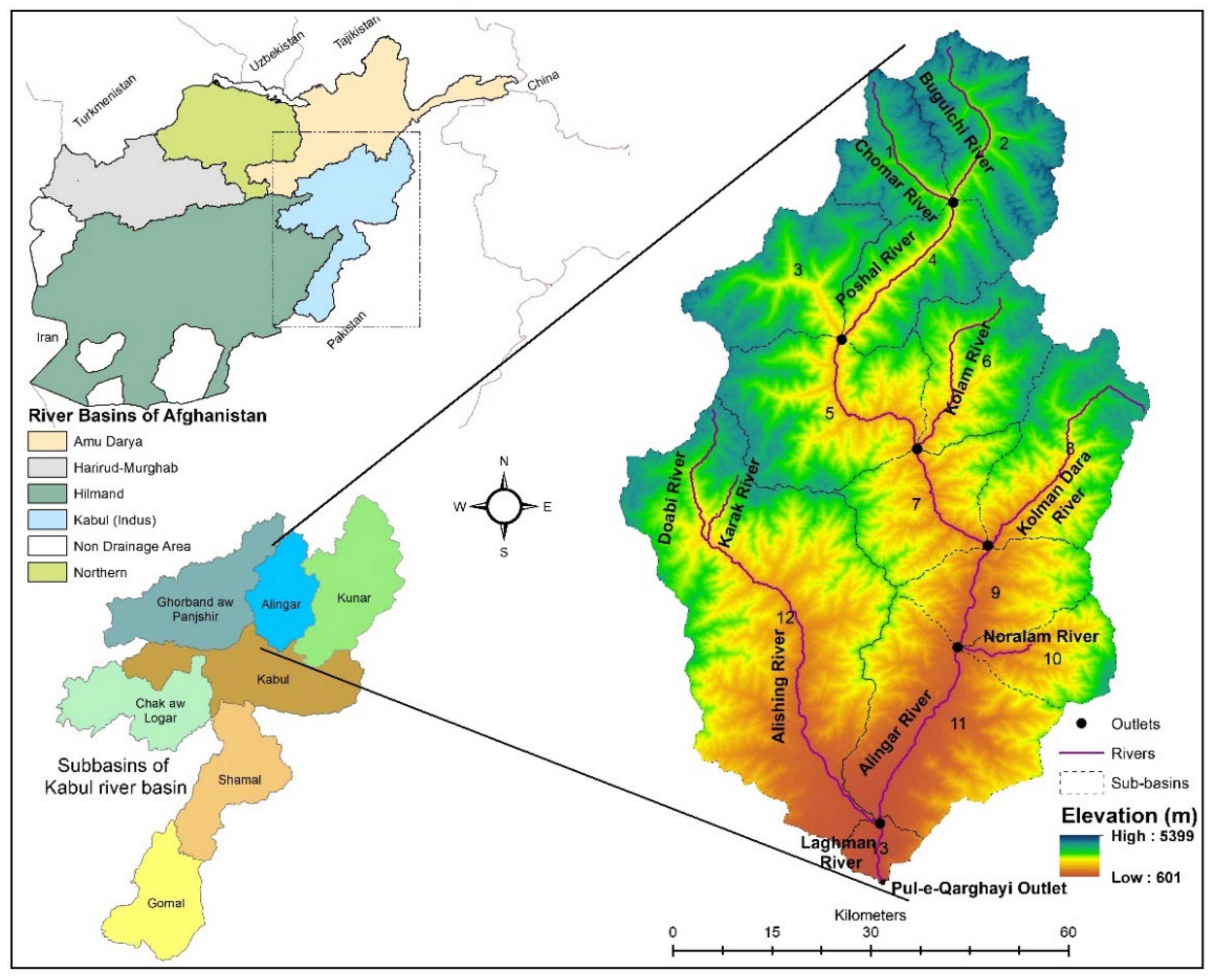
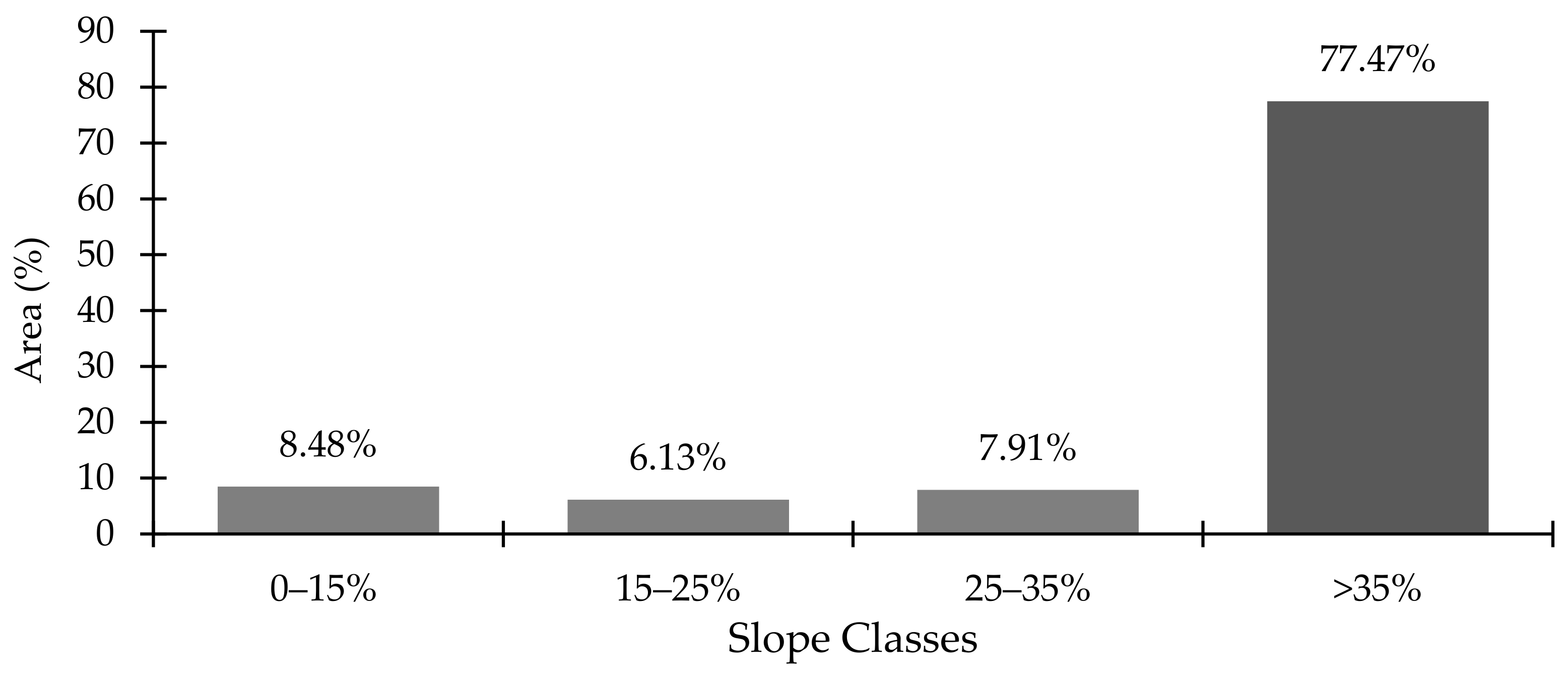
2.1. Study Region

This research was carried out in the Alingar watershed, part of the Kabul River basin (KRB), which is highly heterogeneous in terms of substantial elevation differences between upstream and downstream. The snowmelt’s significant contribution to runoff is therefore prone to the impacts of climate change. This watershed is a typical example of challenging water management tasks due to data-scarce conditions versus the vital need for water allocation considering climate change adaptation, etc. The total area of this basin is about 6239 km², which is further divided into 13 sub-catchments (Figure 1). The elevation range of the study region is from 601 to 5399 m above mean sea level (m.a.s.l.). Based on the Climate Forecast System Reanalysis Survey (CFSR), the mean annual precipitation received at this watershed during the baseline (2000–2019) is around 634 ± 177 mm, while the mean annual temperature observed is about 5.7 °C. The Afghanistan land cover atlas [35] shows that forest and shrubs cover about 31%, rangeland, built-up area, and barren land cover 64%, glaciers cover 0.27%, water bodies cover 1%, and irrigated agriculture covers only 3% of the total area of the watershed. The major rivers flowing in this watershed are the Alingar and Alishing rivers. The tributaries of Alingar are Noralam, Kolman Dara, Kolam, Poshal, Chomar, and Bugulchi rivers, whereas the tributaries of the Alishing river are Doab and Karak rivers. Both the Alingar and Alishing rivers meet at Mihtarlam (Laghman province); the streamflow gauging station is installed at Pul-e-Qarghayi on the Laghman river.

2.2. Assessment of the Performance of the SWAT Model

2.2.1. Description of the SWAT Model

The SWAT is a commonly used semi-distributed and physically-based continuous-time simulation model for quantifying streamflow [36], nutrient transport [37], surface runoff [38], and water demand [39]. The United States Department of Agriculture (USDA) developed and maintains this model regularly, and it works in daily time steps. This model has been used globally in small and medium watersheds [40] to large mountainous watersheds [24]. SWAT has also proven to be very effective in simulating the eventual effects of climate change (CC) scenarios on streamflow [41], erosion [42], and nutrient transport [43], etc. The mathematical expression of the water balance equation, which is the core driving engine of the SWAT model, is given below in Equation (1) [44]:

$$S{W}_t=S{W}_0+{\displaystyle \sum }_{i=1}^t\left(R_{day}-Q_{surf}-E_a-w_{seep}-Q_{gw}\right)$$

(1)

where SW_t represents the final soil water content (mm), SW₀ represents the initial soil water content on the day i (mm), and t represents the time (days). The amount of precipitation on the day i (mm) is R_day, the amount of surface runoff on the day i is shown by Q_surf (mm), E_a is the sum of evapotranspiration (mm) on the day i and Q_gw is the amount of return flow on the day i (mm).

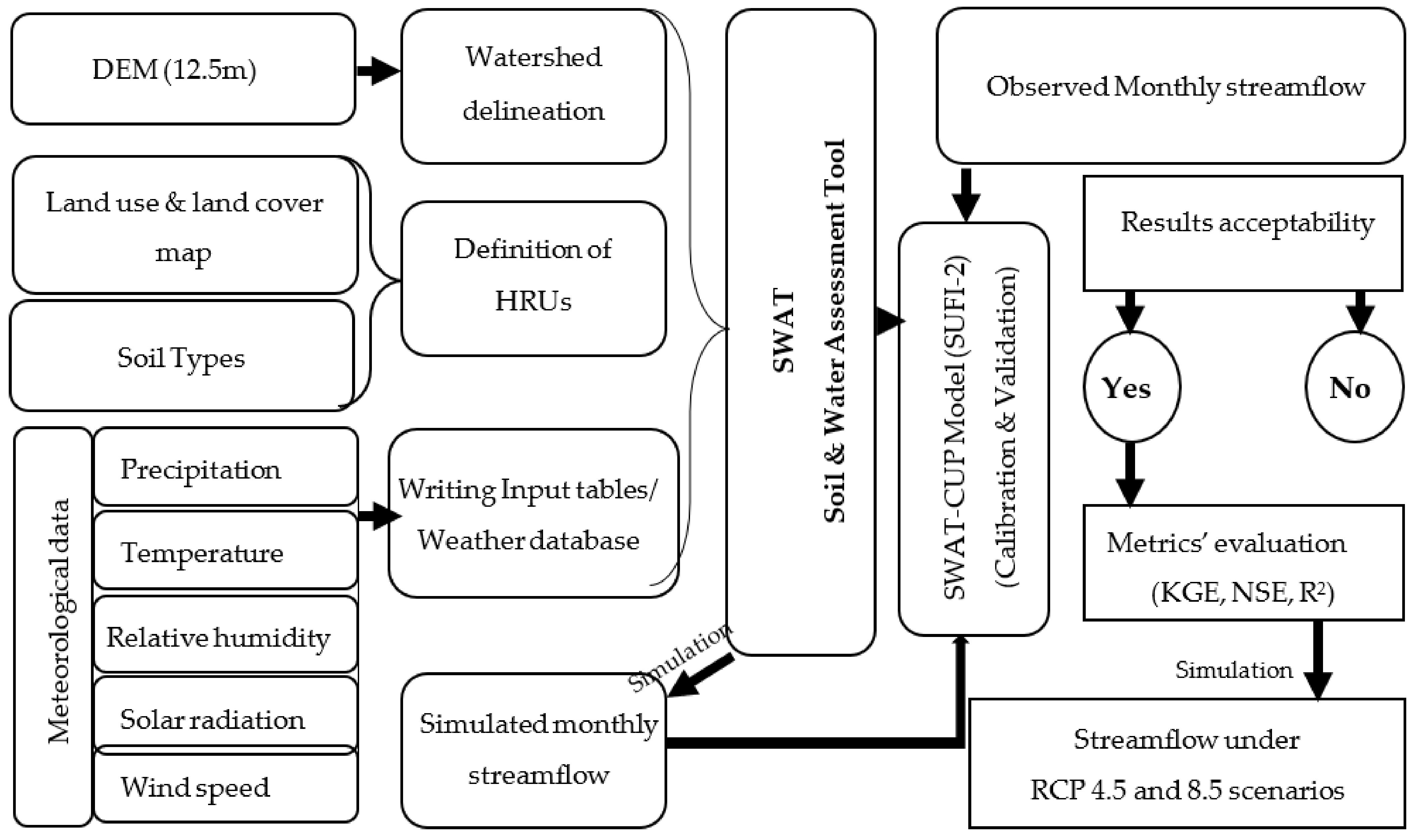
2.2.2. Key Input Data and Methodological Processes Used in the SWAT Model

SWAT is a data-intensive model used for streamflow and other biophysical processes’ simulation in diverse, complex and heterogeneous watersheds. The key datasets used in the SWAT model are the digital elevation model, land use and land cover map, soil map, meteorological and streamflow data. The key processes including data preparation, parametrization, discretization of the subbasins, sensitivity analysis, performance evaluation of metrics and simulation of climate change scenarios etc. has been summarized in the methodological framework (Figure 2).

The summary of the key data used in the SWAT model is given below in

Table 1. Key input data used in the SWAT model.

No	Data Type	Data Attributes	Source of Data
1	Digital elevation model	Elevation	Alaska Satellite Facility https://vertex.daac.asf.alaska.edu (accessed on 17 February 2021).
2	Land use and land cover	Land use	[35]
3	Soil type	Soil characteristics	[45]
4	Meteorological data (CFSR)	Precipitation, Temperature, Solar radiation, Relative humidity and wind speed,	[46]
5	Streamflow data	River discharge	National Water Affairs Regulatory Authority (NWARA)

.

Digital Elevation Model

A digital elevation model (DEM) is a very important and crucial spatial input in the SWAT model used to automatically extract topographic parameters such as slope, elevation, relative relief, aspect, slope-length, etc. A high spatial resolution DEM can be used as the best alternative for conventional surveys and manual evaluation of the topographic conditions of a watershed [47]. Tan et al. [48] investigated the DEM at spatial resolutions ranging from 20 to 500 m and revealed that the DEM’s spatial resolution significantly affects the quality of streamflow computation. Dixon and Earls [49] demonstrated that the DEM’s spatial resolution affects the precision of streamflow estimation through the SWAT model. Moreover, in larger heterogeneous, mountainous, and diversified river basins, the use of higher resolution DEM could be more genuine in watershed delineation to higher accuracy [50]. Therefore, we used an ALOS PALSAR DEM of 12.5 m resolution derived from the Alaska Satellite Facility (ASF) [51]. The elevation across the study region varies between 601–5399 m.a.s.l. (Figure 1). While delineating, 13 sub-basins were formed with the minimum threshold for the sub-basin area of 2000 ha. Using the DEM data, four land slope classes were created i.e 0–15, 15–25, 25–35, and 35–100%. Around 77% of the watershed area was covered by the slope class >35, almost 8% was covered by the slope class 25–35, 6% was covered by the slope class 15–25 and 8.5% was covered by the slope class 0–15% (Figure 3).

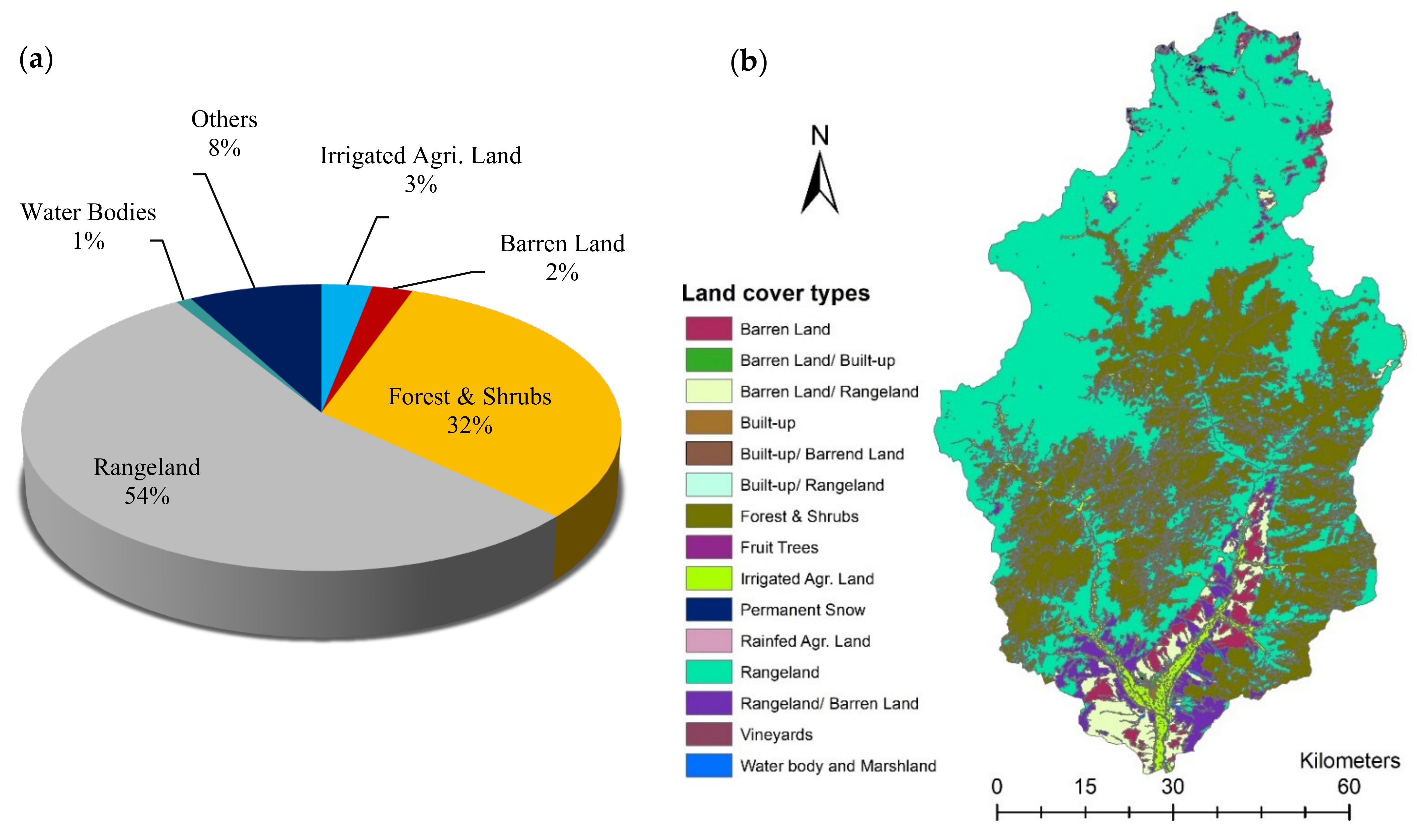
Land Use and Land Cover Map

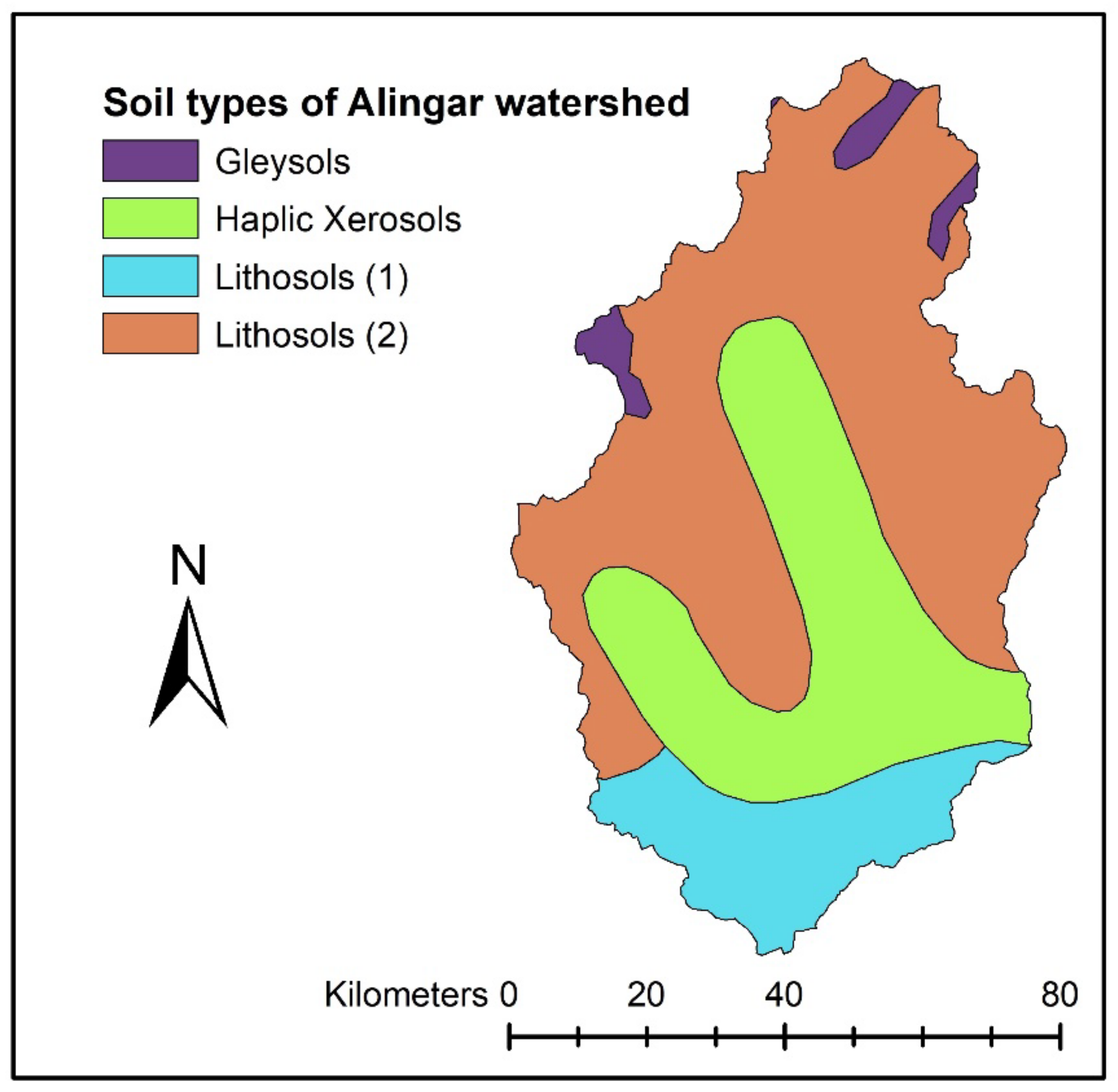
Changes in land use and land cover are critical to the hydrologic cycle [52]. The spatial distribution of different land covers within a watershed is a significant aspect of water balance and is important in inducing the water flux. According to Akhtar et al. [53], there was just a 2% change in the KRB’s agricultural land area from 2003 to 2013, which may not have had a significant influence on the research region’s hydrology. Therefore, we used the FAO land cover map (30 m) [35], which is based on satellite imagery from SPOT-4 and the Global Land Survey (GLS) Landsat Thematic Mapper. The land cover map was resampled to 12.5 m. Around 15 land cover types covered the whole study area; among them, rangeland covers about 54%, forest and shrubs cover approximately 31.5%, while irrigated agricultural land covers around 3% of the study region (Figure 4).

Soil Data

The SWAT model’s hydrological response to the soil properties, reliability of the soil and land use data, as well as the pre-processing procedures used on the geographically dispersed data, is critical to the SWAT model since its internal aggregation procedures have a substantial impact on the original map’s fragmentation and resolution [54]. A comparative analysis of two different resolution soil maps for the SWAT model [55] showed that soil maps with higher resolution yielded better R² and NSE for simulating streamflow and water quality. We used the FAO/UNESCO map [45] in this study and resampled it to 12.5 km to cover the smallest sub-basin. Four dominant soil types represented the entire study region (Figure 5). The major soil type (Lithosols 2), a combination of Lithosols, Cambisols, and Rankers, covers approximately 55% of the study area, Haplic Xerosols cover approximately 29%, Lithosols (1), a combination of Lithosols and Xerosols, covers 13%, and Gleysols covers approximately 3%.

Meteorological Data

Hydrological models require meteorological data to simulate any relevant operation. While this information may be plentiful in some parts of the world, most watersheds and river basins in Afghanistan lack regular meteorological data. The Alingar watershed is one such example where the observed data is limited both in space and time [56]. The two precipitation gauges installed at the extreme outlets at Pul-e-Islamabad and Pul-e-Qarghayi do not represent the upstream’s meteorological conditions, which receive massive precipitation and experience minimum temperatures. Therefore, the use of a global dataset is the only available option in such data-scarce watersheds. The study of Tolera et al. [57] shows that CFSR performed relatively better in the smaller watershed (i.e., Keleta) than in the larger watershed (i.e., Melka Kunture). Therefore, we also used the daily CFSR data of a spatial resolution of 19.2 km while covering the period of 2000–2019; the data was retrieved from the climate engine in CSV (comma-separated values) format for further processing [46].

2.2.3. The SWAT Model’s Calibration, Validation, and Uncertainty Analysis

To diagnose the most sensitive parameters in the streamflow modeling with the SWAT model, the Uncertainty in Sequential Uncertainty Fitting (SUFI-2) algorithm in SWAT Calibration and Uncertainty Procedures (SWAT-CUP) was utilized, which generates Latin Hypercube samples for sensitivity analyses. For calibrating the SWAT model for those watersheds which are snow-fed, it is important to consider snow relevant parameters, e.g., Snowfall temperature (°C) (SFTMP), Snowmelt base temperature (°C) (SMTMP), Maximum snowmelt factor (SMFMX, mm of water/°C day⁻¹), Minimum snowmelt factor (SMFMN, mm of water/°C day⁻¹) and Snowpack temperature lag factor (TIMP), and runoff relevant parameters, e.g., the soil permeability, land use, and antecedent soil-water conditions that all influence the SCS curve number, soil water content (SOL_AWC) as well as soil evaporation compensation factor (ESCO) [58]. We used the SUFI-2 algorithm in the SWAT-CUP to calibrate, validate, and analyze the sensitivity of the SWAT model [27]. The SWAT model’s simulation accuracy was assessed using the monthly observed streamflow data collected from the Pul-e-Qarghayi station. Based on the limited streamflow data availability, the calibration period was 2008–2013, and the validation period was 2014–2019. Via an iterative method, the SUFI-2 algorithm calculates the range of the 95PPU and brackets the actual streamflow data points within the band, which is called the r-factor [59]. The algorithm uses two main metrics to determine the goodness of fit, i.e., (1) the p-factor, which ranges from 0 to 1, and (2) the r-factor, which is the average 95PPU-band’s width ratio to the observed variable’s standard deviation [59]. After obtaining appropriate KGE, NSE, and R², the parameter ranges thus yielded in the last iteration were considered the calibrated parameters for the validation of the SWAT model.

2.3. Evaluation of Different Statistical Metrics

While evaluating hydrological models, the performance criteria are used as a single number to show the similarities between simulated and observed streamflow [25]. In this study, we used the KGE [25] as the objective function with the SUFI-2 algorithm for automatic calibration. The minimum threshold of the objective function (i.e., the KGE) for the behavioral solutions was set to be 0.50. The mathematical expression of these metric indicators is given below:

$$KGE=1-\sqrt{{\left(\alpha -1\right)}^2+{\left(r-1\right)}^2+{\left(\beta -1\right)}^2}$$

(2)

where the linear correlation between actual and simulated data is expressed by r, the metric of the streamflow variability error is denoted by α, and the bias is shown by β.

The performance of the model is considered reasonable when −0.41 < KGE < 1 [60]. Similarly, NSE [61] and R² are the byproducts automatically calculated by the SWAT-CUP model by comparing the observed and simulated streamflow. The NSE is calculated by using Equation (3), as given below:

$$NSE=1-\frac{{{\displaystyle \sum }}_{i=0}^n{(Q_{obs,i}-Q_{sim,i})}_i^2}{{{\displaystyle \sum }}_{i=0}^n{(Q_{obs,i}-{\overline{Q}}_{obs} )}_i^2}$$

(3)

where $Q_{obs}$ denotes the actual streamflow, $Q_{sim}$ denotes the simulated streamflow and ${\overline{Q}}_{obs}$ denotes the observed mean streamflow and $n$ is the total number of observations.

NSE is varying between −∞ and 1, when the NSE = 1, it is considered to be the optimal simulation. Values between 0 and 1 are typically considered acceptable levels of performance; however, a value below 0 means that the mean observed streamflow is a better predictor than the simulated streamflow, showing unsatisfactory performance. Similarly, the degree of collinearity between observed and simulated streamflow is denoted by R². It indicates the fraction of the variance in observed streamflow that the model explains. The value of R² ranges from 0 to 1, with higher values suggesting less error variation, and values larger than 0.5 are normally regarded as acceptable [24]. The coefficient of determination (R²) is calculated using the following equation:

$$R^2=\frac{{\left[{{\displaystyle \sum }}_{i=1}^n\left(Q_{obs,i}-{\overline{Q}}_{obs}\right)\left(Q_{sim,i}-{\overline{Q}}_{sim}\right) \right]}^2}{{{\displaystyle \sum }}_{i=1}^n\left(Q_{obs,i}-{\overline{Q}}_{obs} \right){ }^2 {{\displaystyle \sum }}_{i=1}^n\left(Q_{sim,i}-{\overline{Q}}_{sim}\right){ }^2}$$

(4)

where $n$ is the total number of observations, $Q_{obs}$ and $Q_{sim}$ show the observed and simulated streamflow, and ${\overline{Q}}_{obs}$ and ${\overline{Q}}_{sim}$ and are the observed and simulated mean streamflow, respectively.

2.4. Analysis of the Streamflow under Changing Climate

The CORDEX (Coordinated Regional Downscaling Experiment) provides the expected changes in numerous variables under the climate change (CC) scenarios [62]. The data (50 km spatial resolution) was retrieved using the regional circulation model (RegCM4-4) from the South Asia domain of the CORDEX. For analyzing the impacts of CC on streamflow from 2020 to 2045, the daily maximum and minimum temperature and precipitation data were downloaded from the CORDEX domain. The study region is expected to receive mean annual precipitation of 774 ± 229 and 789 ± 203 mm during 2020–2045, respectively, under the RCP 4.5 and 8.5. Similarly, the mean annual temperature under the RCP 4.5 and 8.5 during 2020–2045 is predicted to be 5.5 and 5.8 °C, respectively (Figure 6). The future streamflow was analyzed in annual (i.e., minimum, and mean) and monthly time steps to diagnose major shifts at seasonal scales to relate these temporal changes at the water supply side to periods of peak demand for agricultural purposes.

3. Results and Discussion

During the calibration procedure, the highest absolute t-Stat value is attributed to the highest sensitivity of that specific parameter during calibration [27]. In the present study, the sensitivity analysis tool in the SWAT-CUP model identified eight parameters as being the most sensitive (

Table 2. List of the hydrologic parameters used in calibration and their respective value ranges and ranking.

Sensitivity Rank	* Parameter Name	Fitted Value	Min Value	Max Value	t-Stat	p-Value
1	V__SMFMX.bsn	0.151367	0	5	−57.55	0.0000
2	V__SMFMN.bsn	0.375977	0	5	11.95	0.0000
3	R__CN2.mgt	0.000635	−0.15	0.1	−11.05	0.0000
4	V__ESCO.hru	0.305957	0.2	0.7	−3.77	0.0002
5	R__SOL_AWC(..).sol	−0.203369	−0.25	0	3.55	0.0004
6	V__SFTMP.bsn	0.410156	−2	2	−3.22	0.0014
7	V__SMTMP.bsn	0.894531	−2	2	−2.80	0.0053
8	V__TIMP.bsn	0.254199	0.2	0.7	0.49	0.6237

* SMFMX is short for maximum snowmelt factor, SMFMN is abbreviated from minimum snowmelt factor, SCS is short for the soil conservation service, CN is runoff curve number, ESCO is the short form of soil evaporation compensation factor, SOL_AWC is available water capacity of the soil layer, SFTMP is short for snowfall temperature. SMTMP denotes Snowmelt base temperature and TIMP is abbreviated for lag factor for snow-pack temperature.

). Following the identification of the sensitive parameters, we calibrated their values while the default model values of other parameters were retained throughout the calibration process. The streamflow was sensitive to maximum snowmelt factor (SMFMX), minimum snowmelt factor (SMFMN), the soil conservation service (SCS)’ runoff curve number (CN2), soil evaporation compensation factor (ESCO), an available water capacity of the soil layer (SOL_AWC), snowfall temperature (SFTMP), Snowmelt base temperature (SMTMP), and lag factor for snowpack temperature (TIMP).

The KGE, the selected objective function, acquired during iterations for the SWAT model’s calibration at the Pul-e-Qarghayi outlet was 0.72, NSE was 0.59, and R² was 0.60, which can be classified as “moderate” to “good according to Thiemig” [63]. During validation of the SWAT model (after considering the new values of the sensitive parameters) the KGE increased to 0.89, while NSE and R² increased to 0.98 each (Figure 7).

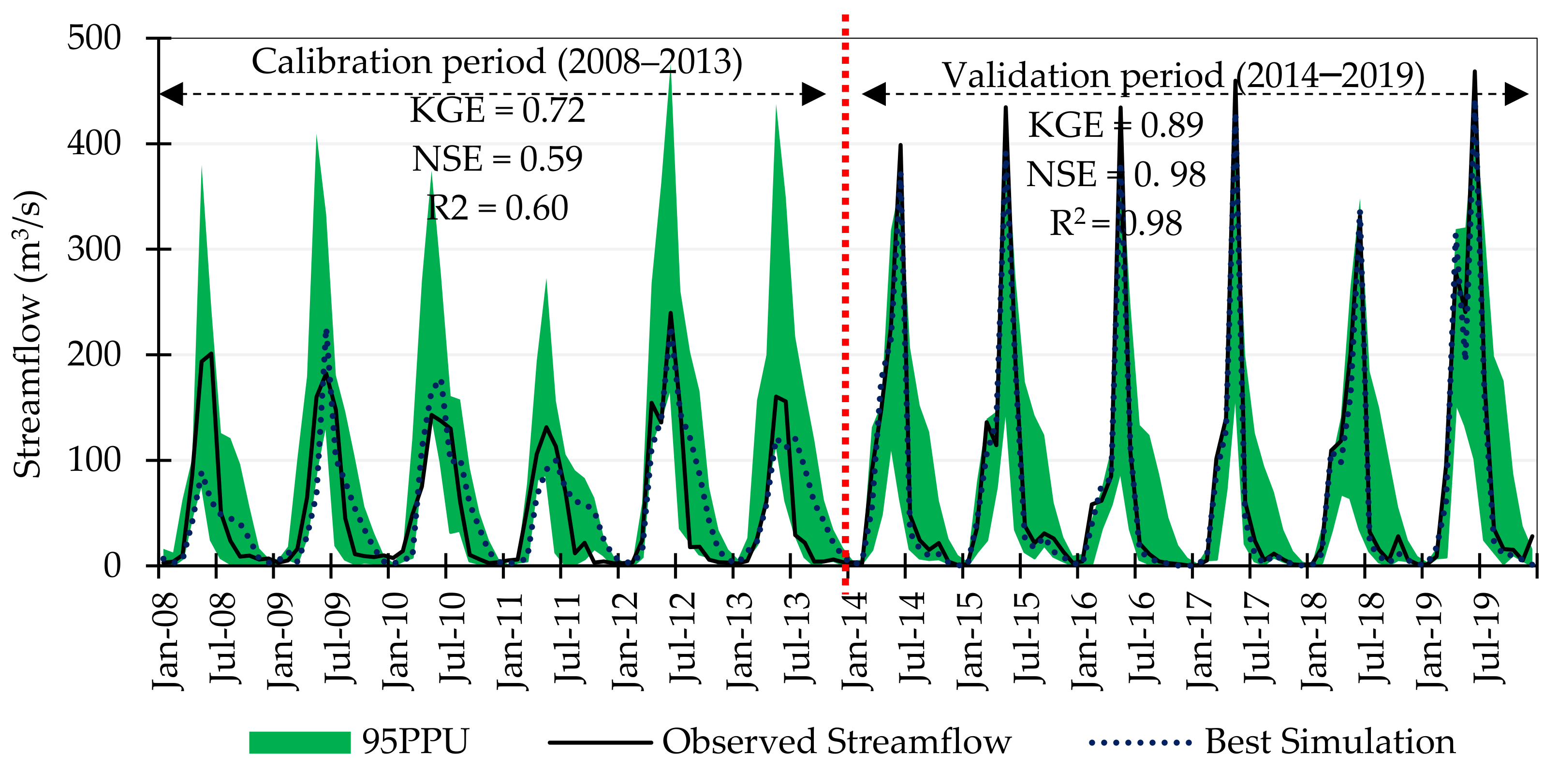
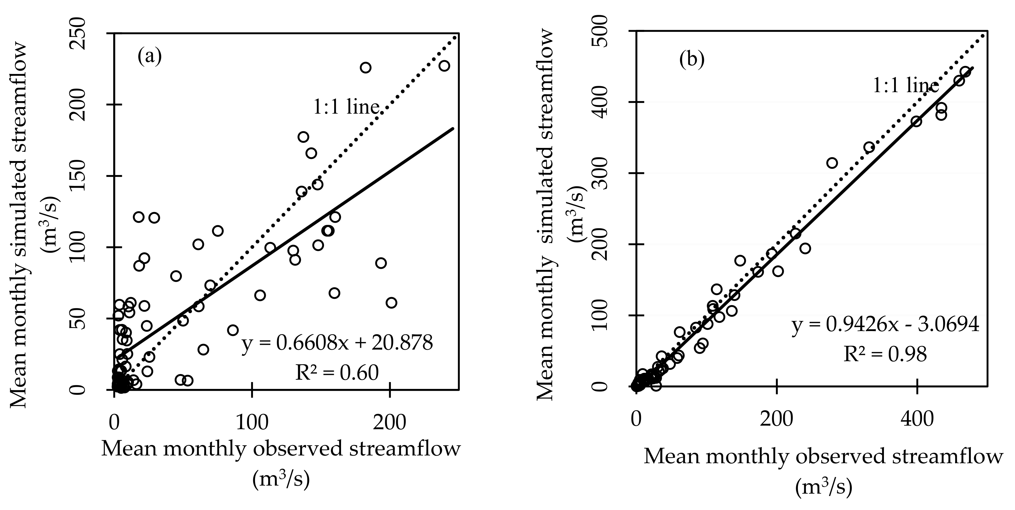
3.1. Performance Evaluation of the Statistical Metrics

During iterations for calibration of the SWAT model at the Pul-e-Qarghayi outlet, the KGE achieved was 0.72, the NSE was 0.59, and R² was 0.60 (Figure 7). The mean annual simulated streamflow during calibration was 54.53 ± 53.69 m³/s, while for the same period the mean annual observed streamflow was 50.93 ± 63.06 m³/s. During the calibration, the p- and r-factors were 0.86 and 1.58, respectively. During calibration, there has been considerable improvement in the p-factor (i.e., 0.92) which shows that 92% of the observed data points have been successfully bracketed during the simulations. In contrast, the r-factor reduced from 1.58 (during calibration) to 0.83 (during validation), which shows considerable model development in simulating the streamflow at monthly time intervals. As a result, the KGE improved from 0.72 (during calibration) to 0.89 (during validation). Similarly, the NSE increased from 0.59 (during calibration) to 0.98 (during validation), reflecting a considerable development in the model’s prediction of the streamflow. Improvement has been observed in the RSR value, which reduced from 0.64 (during calibration) to 0.14 during validation. During the validation period, the mean annual simulated and observed streamflow were 73.81 ± 115.40 and 81.56 ± 121.58, respectively, which are close to each other. Further statistical details are found in

Table 3. Summary of the performance evaluation metrics’ statistics during calibration and validation.

	p-Factor	r-Factor	R2	NSE	PBIAS	KGE	RSR	VOL_FR	Mean Annual SSF (Mean Annual OSF) (m3/s)	STD_S (STD_O)
Calibration	0.86	1.58	0.600	0.59	−7.1	0.72	0.64	0.93	54.53 (50.93)	53.69 (63.06)
Validation	0.92	0.83	0.986	0.98	9.5	0.89	0.14	1.11	73.81 (81.56)	115.40 (121.58)

Note: p—factor refers to the percentage of observations covered by the 95PPU, r—factor depicts the thickness of the 95PPU, R², is the coefficient of determination, NSE is the Nash—Sutcliffe Efficiency, PBIAS is the Percent bias, KGE is the Kling–Gupta Efficiency, RSR is the ratio of the RMSE and standard deviation, VOL_FR is the fraction of the overall water balance which is predicted, Mean annual SSF refers to mean annual simulated streamflow, Mean annual OSF refers to mean annual observed streamflow, STD_S refers to Simulated standard deviation and STD_O refers to Observed standard deviation,.

. The mean annual simulated and observed streamflow increased by around 35% and 29% in the validation period compared to the calibration period, respectively; this increase was caused by a 123% and 41% increase in total monthly precipitation, especially in the months of February and March.

According to Thiemig [63], the simulations’ performance can be grouped as intermediate when 0.75 > KGE > 0.5 and good when KGE > 0.75; according to Moriasi et al. [19], the scatter plots shown in Figure 8 depict a satisfactory result for calibration where 0.50 < NSE < 0.65, whereas for validation the NSE values are very good, i.e., 0.75 < NSE < 1.00. According to Knoben et al. [60], if the mean streamflow was used as a benchmark, model output in the range of −0.41 < KGE ≤ 1 may be considered “reasonable” as the model outperforms the benchmark; based on this, the KGE was 0.72 during calibration and 0.89 during validation, which rationalizes the model’s performance as acceptable. A SWAT model was also used in Pakistan at the Simly Dam watershed, and while evaluating the model’s performance, an NSE of 0.85 and 0.79 for validation were yielded for calibration and validation periods respectively [64]. Another similar experiment by Shrestha et al. [65] shows that R² values were 0.67 and 0.75 while NSE values were 0.63 and 0.74 during calibration (1984–1993) and validation periods (1994–2001), respectively [65]. Zare et al. [66] evaluated soil water content through the SWAT model for Southern Saskatchewan (SK, Canada) and achieved NSE of 0.62 and 0.78, during calibration and validation (of streamflow) respectively. Son et al. [67] calibrated and validated the SWAT model with streamflow in the Nam Rom catchment (Vietnam), and the NSE achieved during calibration and validation was 0.76 and 0.64.

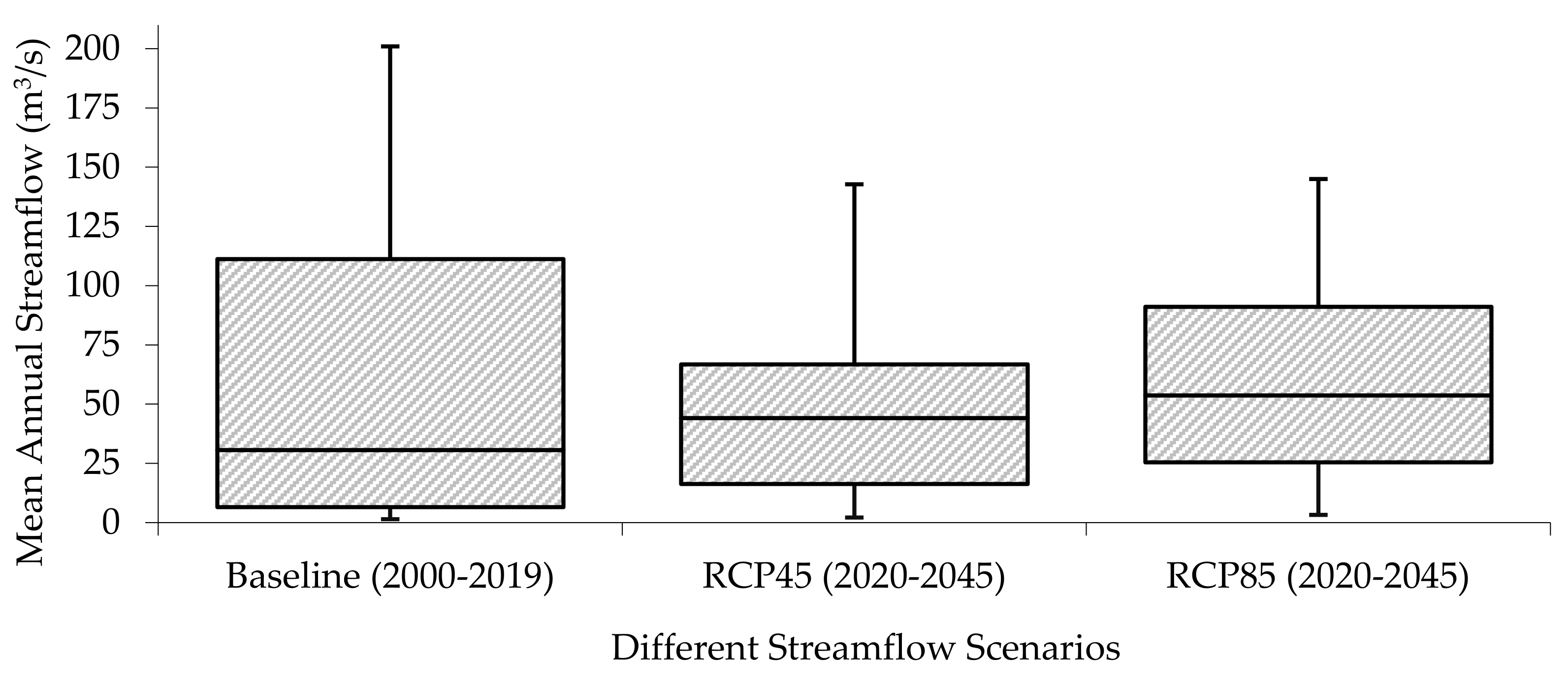
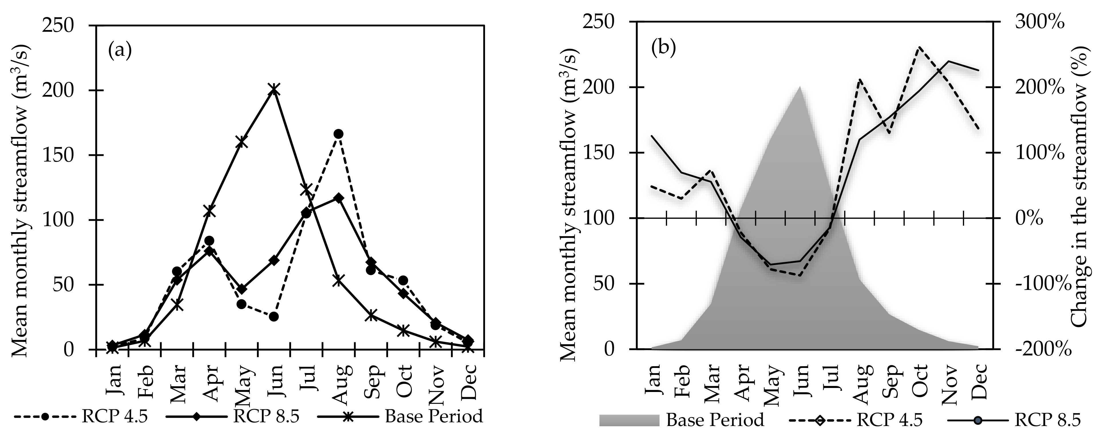
3.2. Temporal Analysis of the Variation in Streamflow under Changing Climate from 2020 to 2045

The mean annual streamflow during the base period (2000–2019) was 61.48 ± 69.0 m³/s, while it was 52.12 ± 48.3, and 51.87 ± 37.3 m³/s under the RCP 4.5 and 8.5 (2020–2045), respectively (Figure 9). There was not much difference between the mean annual streamflow under both CC scenarios; however, we recorded high variability under the based period and RCP 4.5. The statistical evaluation of the annual streamflow shows that by 2045, approximately a 15 and 16% reduction in the mean annual streamflow is expected under RCP 4.5 and 8.5, respectively.

Table 4. Projected changes (%) in the annual mean, minimum, and maximum streamflow (m³/s) under the RCP 4.5 and 8.5 in comparison to the base period.

Period	Annual Minimum Streamflow (m3/s)	Change from Baseline (%)	Annual Maximum Streamflow (m3/s)	Change from Baseline (%)	Annual Mean Streamflow (m3/s)	Change from Baseline (%)
Base Period (2000–2019)	1.45	-	200.1	-	61.5	-
RCP 4.5 (2020–2045)	2.15	48.2	166.3	−17.2	52.1	−15.2
RCP 8.5 (2020–2045)	3.27	125.6	117.0	−41.8	51.9	−15.6

summarizes the mean annual variation in the streamflow compared to the base period; the annual minimum streamflow under scenarios RCP 4.5 and 8.5 are expected to increase by 48.2 and 125.6%, respectively. The annual maximum streamflow is projected to decrease by 17.2 and 41.8%, respectively. Similarly, the annual mean streamflow is projected to decrease by 15.2 and 15.6%, respectively.

Figure 10 depicts that the peak hydrograph under the base period is usually in June when increased temperature melts down most of the accumulated snow on the upstream heights of the watershed. Under the CC scenarios, the peak hydrograph is expected to split into two peaks, one formed in Mar-Apr which indicates earlier snowmelt, and the second one in August, which is due to an increase in summer or Monsoon rains contrary to the base period, which is adding to the peak hydrograph in August. The comparative analysis of the monthly streamflow under the RCP 4.5 shows that streamflow in January, February, and March increased by 48, 30, and 74%, respectively. With 262 and 207%, the highest increase is projected for October and November, respectively. Under the same scenario (i.e., RCP 4.5), the mean streamflow in May and June is expected to decrease by 78 and 87%, respectively. Likewise, under the RCP 8.5, streamflow in November, December and January is expected to increase by 240, 226, and 126%, respectively; this change can be explained by a partial shift from snowfall to rain (as a consequence of higher temperature) or by snow melting periods in winter. Conversely, the highest decrease is projected for May and June by 71 and 66%, respectively. Overall, the shift in hydrograph is similar under both scenarios.

3.3. The Impact of Spatial Scale on the Performance of the SWAT Model

The calibration of the SWAT model for multi outlets, especially in large river basins under highly heterogenic conditions of land use, soil types, climate, and elevation differences, is quite challenging [68]. This is because if one outlet is being calibrated for a targeted objective function, any increase in any variable may equally influence the streamflow (by decreasing or increasing the hydrograph peak), actual evapotranspiration, and runoff generation as well as other water balance components [69]. Therefore, as a standard iteration exercise, it is challenging to achieve a common range of sensitive parameters, which boosts the calibration results equally [70,71]. Therefore, in this study, we used the KGE, which incorporates the model’s bias, temporal fitness, and variability instead of NSE, which underestimates the variability in the simulated streamflow [25]. Moreover, to evaluate the SWAT model’s performance at a single outlet in the Alingar watershed, i.e., Pul-e-Qarghayi, the results were compared to the SWAT model’s performance at multi-outlets, which included Pul-e-Qarghayi together with five other outlets reported in Akhtar et al. [12], while ensuring that there are no storage structures or large diversions upstream of the specified outlets that might affect the volume of river discharge.

Table 5. Evaluation results of single-outlet and multi-outlet simulation effect.

Simulation Type	Performance Metrics’ Value Range (Multi-Outlet Simulation)		Period	Performance Metrics’ Value Range (Single Outlet Simulation)			Period
	NSE	R2		KGE	NSE	R2
Calibration	0.74	0.79	2008–2010	0.72	0.59	0.60	2008–2013
Validation	0.62	0.86	2011–2013	0.89	0.98	0.98	2014–2019

reveals that the KGE (as the chosen objective function) yielded a value of 0.72 (during calibration) and 0.89 (during validation), which according to Thiemig [63] can be classified as intermediate to good performance. During calibration, the NSE achieved was 0.59, which suddenly increased to 0.98 (during validation) and indicated a perfect correspondence between the observed and simulated streamflow per the criteria suggested by Moriasi et al. [19] and highlighted estimation error variance almost equal to 2%.

The SWAT model’s calibration for a single outlet improved the model’s performance by increasing the objective function and other relevant performance metrics and confined the list of sensitive parameters that are very much specific to the physiographic conditions of the rather smaller watershed with a single outlet.

Table 6. A comparative analysis of the parameters used for sensitivity while simulating streamflow at multi and single outlets.

Sensitive Parameters for Calibrating Multi-Outlets at the KRB Including Pul-e-Qarghayi Streamflow Measurement Station of Alingar Watershed					Sensitive Parameters for Calibrating Single Outlet at Pul-e-Qarghayi Streamflow Measurement Station of Alingar Watershed
Sensitivity Rank	Parameter	Fitted Value	Min Value	Max Value	Sensitivity Rank	Parameter	Fitted Value	Min Value	Max Value
1	* r__CN2.mgt	−0.49	−0.49	−0.48	1	v__SMFMX.bsn	0.1513	0	5
2	r_SOL_BD(..).sol	−0.02	−0.02	−0.01	2	v__SMFMN.bsn	0.3759	0	5
3	** v__ALPHA_BF.gw	0.19	0.18	0.22	3	r__CN2.mgt	0.0006	−0.15	0.1
4	v__GW_DELAY.gwwww	160.64	160.34	166.11	4	v__ESCO.hru	0.3059	0.2	0.7
5	v__REVAPMN.gw	19.89	19.51	19.93	5	r__SOL_AWC(..).sol	−0.203	−0.25	0
6	v__GWQMN.gw	43.49	43.43	44.24	6	v__SFTMP.bsn	0.4101	−2	2
7	v__EPCO.bsn	0.28	0.27	0.28	7	v__SMTMP.bsn	0.8945	−2	2
8	v__ESCO.bsn	0.49	0.44	0.5	8	v__TIMP.bsn	0.2541	0.2	0.7
9	v__CH_N2.rte	0.19	0.18	0.19
10	v__SMTMP.bsn	−3.61	−3.7	−3.55
11	v__SMFMX.bsn	13.41	12.55	13.6
12	v__SMFMN.bsn	8.9	8.55	9.25
13	v__TIMP.bsn	0.15	0.15	0.16
14	v__SURLAG.bsn	1.76	1.52	1.97

* r means an existing parameter value is multiplied by (1+ a given value), ** v__ means the existing parameter value is to be replaced by a given value. SOL_BD refers to soil bulk density (g/cm³), ALPHA_BF is baseflow alpha factor (1/day), GW_DELAY shows groundwater delay time (days), GWQMN is the threshold depth of water in the shallow aquifer required for return flow to occur (mm H₂O), REVAPMN is the threshold water depth in shallow aquifer for “revap” or percolation to occur (mm), GWQMN is threshold depth of water in the shallow aquifer needed for return flow to occur (mm H₂O), EPCO is the plant uptake compensation factor, CH_N2 is the hydraulic conductivity of the main channel (mm/h) and SURLAG is the surface runoff lag coefficient.

shows that the fitted values for the common parameters under both single and multi-outlets-based calibration have considerably changed. The reason behind this is that any parametric values under multi outlets are strongly driven by the spatial heterogeneity of parameters, errors incurring during the acquisition of hydrological data, and errors resulting from optimizing the model’s behavior that reach a compromise between the different outlets [69]. Besides, calibrating multi-outlets at spatially large and heterogenic watersheds is computationally intensive [72]. Likewise, the sensitivity ranking has also changed with a greater difference. The number of parameters used in the calibration phase was reduced while calibrating at a single outlet, and simulation performance was also improved by selecting spatially homogenous parameters. The results of this study are in line with a similar study from the Yellow River, where the comparative performance did not change, but the number of sensitive parameters did [10].

4. Conclusions

The performance of NSE, as an objective function, was poor for both single and multi-outlets. However, the KGE performed better when used as an objective function for streamflow estimation by using the SWAT model. The NSE values improved many times as the KGE value increased. The KGE is recommended as the best performance indicator and an alternative to NSE for multi-outlets simulation, especially under a heterogeneous environment. The KGE is based upon the balanced optimization of the model’s bias, temporal fitness, and variability. While using the KGE, low values were well expressed for correlation and bias present in the data compared to the NSE, which didn’t perform well, especially under low streamflow conditions.

The SWAT model’s performance is compromised at multi outlets in large river basins; this is more evident especially under physiographically and climatically large and heterogeneous river basins. Therefore, to overcome these shortcomings during model evaluation, it is recommended to test the SWAT model’s performance at the individual outlet. Moreover, simulating multi-outlets is computationally intensive to achieve the desired objective function for enhanced performance of hydrological modeling. For hydrological models’ performance in regions with higher heterogeneity in climatic and physiographic conditions, land cover, cropping pattern, streamflow, etc., using the KGE as a performance metric in combination with R², p- and r-factors enhances the SWAT model’s simulation performance.

The modeling of CC scenarios demonstrates that the mean annual streamflow under RCPs 4.5 and 8.5 is not much different from each other. Under these scenarios, the model project will see a 15.2% to 15.6% decline in mean annual streamflow by 2045 under the RCPs 4.5 and 8.5, respectively. The results of Akhtar et al. [73] have also demonstrated the decreasing trend in groundwater storage not only in the KRB but also across the entire Indus Basin; the groundwater storage is directly linked to the amount of surface water flow as well as anthropogenic interventions that hamper the groundwater recharge as well as accelerate unsustainable groundwater withdrawal. The mean monthly minimum streamflow is anticipated to rise by 48.2% and 125.6% under the RCP 4.5 and 8.5, respectively; the monthly maximum streamflow is expected to fall by 17.2% and 41.8%, respectively. Furthermore, the peak hydrograph is expected to split into two peaks: one in March-April, indicating earlier snowmelt, and the second peak in August, indicating that the increase in summer or Monsoon rains, contrary to the base period, is contributing to the peak hydrograph in August. The information on a simulated considerable decrease of streamflow in the period from May until July and the increase from August until December can support water management in conceiving adaptation strategies in terms of (i) re-arranging irrigation schedules (and eventually even cropping patterns) towards lower water availability in the beginning and middle of the cropping season and higher water availability in the late season, and (ii) considering the introduction of facilities to store a part of the increased runoff at the end of and after the vegetation period for utilization in agriculture during demand periods taking into account the effects of changing low flow conditions on ecology.

References

1. Elfeki, A.; Masoud, M.; Niyazi, B. Integrated rainfall–runoff and flood inundation modeling for flash flood risk assessment under data scarcity in arid regions: Wadi Fatimah basin case study, Saudi Arabia. Nat. Hazards 2017, 85, 87–109. [Google Scholar] [CrossRef]
2. Alipour, M.; Kibler, K.M. Streamflow prediction under extreme data scarcity: A step toward hydrologic process under-standing within severely data-limited regions. Hydrol. Sci. J. 2019, 64, 1038–1055. [Google Scholar] [CrossRef]
3. Pilgrim, D.H.; Chapman, T.G.; Doran, D.G. Problems of rainfall-runoff modelling in arid and semiarid regions. Hydrol. Sci. J. 1988, 33, 379–400. [Google Scholar] [CrossRef]
4. Brunner, G.W. HEC-RAS River Analysis System. Hydraulic Reference Manual; Version 1.0.; Hydrologic Engineering Center: Davis, CA, USA, 1995. [Google Scholar]
5. Khadka, J.; Bhaukajee, J. Rainfall-Runoff Simulation and Modelling Using HEC-HMS and HEC-RAS Models: Case Studies from Nepal and Sweden; TVVR 18/5009; Lund University: Lund, Sweden, 2018. [Google Scholar]
6. Kjeldsen, T.; Stewart, E.J.; Packman, J.C.; Folwell, S.S.; Baylis, A.C. Revitalisation of the FSR/FEH Rainfall Runoff method. Final Report to DEFRA/EA. 2005, CEH, Wallingford, UK. Available online: https://assets.publishing.service.gov.uk/media/602ba561e90e070562513e33/Revitalisation_of_the_FSRFEH_rainfall_runoff_method_technical_report.pdf (accessed on 22 February 2022).
7. Joo, J.; Kjeldsen, T.; Kim, H.J.; Lee, H. A comparison of two event-based flood models (ReFH-rainfall runoff model and HEC-HMS) at two Korean catchments, Bukil and Jeungpyeong. KSCE J. Civ. Eng. 2014, 18, 330–343. [Google Scholar] [CrossRef]
8. Cunderlik, J. Hydrologic Model Selection for the CFCAS Project: Assessment of Water Resources Risk and Vulnerability to Changing Climatic Conditions; Department of Civil and Environmental Engineering, The University of Western Ontario: London, ON, Canada, 2003. [Google Scholar]
9. Arnold, J.G.; Srinivasan, R.; Muttiah, R.S.; Williams, J.R. Large area hydrologic modeling and assessment Part I: Model Development. JAWRA J. Am. Water Resour. Assoc. 1998, 34, 73–89. [Google Scholar] [CrossRef]
10. Li, K.; Wang, Y.; Li, X.; Yuan, Z.; Xu, J. Simulation effect evaluation of single-outlet and multi-outlet calibration of Soil and Water Assessment Tool model driven by Climate Forecast System Reanalysis data and ground-based meteorological station data—A case study in a Yellow River source. Water Supply 2021, 21, 1061–1071. [Google Scholar] [CrossRef]
11. Rajib, M.A.; Merwade, V.; Yu, Z. Multi-objective calibration of a hydrologic model using spatially distributed remotely sensed/in-situ soil moisture. J. Hydrol. 2016, 536, 192–207. [Google Scholar] [CrossRef] [Green Version]
12. Akhtar, F.; Awan, U.K.; Borgemeister, C.; Tischbein, B. Coupling Remote Sensing and Hydrological Model for Evaluating the Impacts of Climate Change on Streamflow in Data-Scarce Environment. Sustainability 2021, 13, 14025. [Google Scholar] [CrossRef]
13. Zhang, X.; Srinivasan, R.; Arnold, J.; Izaurralde, R.C.; Bosch, D. Simultaneous calibration of surface flow and baseflow simulations: A revisit of the SWAT model calibration framework. Hydrol. Process. 2011, 25, 2313–2320. [Google Scholar] [CrossRef]
14. Pfannerstill, M.B.; Guse, B.; Fohrer, N.B. Smart low flow signature metrics for an improved overall performance evaluation of hydrological models. J. Hydrol. 2014, 510, 447–458. [Google Scholar] [CrossRef]
15. Fujita, T.; de Morais, M.V.B.; Dos Santos, V.C.; Rudke, A.P.; de Eiras, M.M.; Xavier, A.C.F.; Rafee, S.A.A.; Santos, E.B.; Martins, L.D.; Uvo, C.B.; et al. Simulating Discharge in a Non-Dammed River of Southeastern South America Using SWAT Model. Water 2022, 14, 488. [Google Scholar] [CrossRef]
16. Adhikary, P.P.; Sena, D.R.; Dash, C.J.; Mandal, U.; Nanda, S.; Madhu, M.; Sahoo, D.C.; Mishra, P.K. Effect of Calibration and Validation Decisions on Streamflow Modeling for a Heterogeneous and Low Runoff–Producing River Basin in India. J. Hydrol. Eng. 2019, 24, 05019015. [Google Scholar] [CrossRef]
17. Chilkoti, V.; Bolisetti, T.; Balachandar, R. Multi-objective autocalibration of SWAT model for improved low flow performance for a small snowfed catchment. Hydrol. Sci. J. 2018, 63, 1482–1501. [Google Scholar] [CrossRef]
18. Willmott, C.J. On the validation of models. Phys. Geogr. 1981, 2, 184–194. [Google Scholar] [CrossRef]
19. Moriasi, D.N.; Arnold, J.G.; van Liew, M.W.; Bingner, R.L.; Harmel, R.D.; Veith, T.L. Model evaluation guidelines for systematic quantification of accuracy in watershed simulations. Trans. ASABE 2007, 50, 885–900. [Google Scholar] [CrossRef]
20. Legates, D.R.; McCabe, G.J., Jr. Evaluating the use of “goodness-of-fit” measures in hydrologic and hydroclimatic model validation. Water Resour. Res. 1999, 35, 233–241. [Google Scholar] [CrossRef]
21. Pushpalatha, R.; Perrin, C.; Le Moine, N.; Andréassian, V. A review of efficiency criteria suitable for evaluating low-flow simulations. J. Hydrol. 2012, 420–421, 171–182. [Google Scholar] [CrossRef]
22. Osuch, M.; Romanowicz, R.J.; Booij, M.J. The influence of parametric uncertainty on the relationships between HBV model parameters and climatic characteristics. Hydrol. Sci. J. 2015, 60, 1299–1316. [Google Scholar] [CrossRef] [Green Version]
23. Garcia, F.; Folton, N.; Oudin, L. which objective function to calibrate rainfall–runoff models for low-flow index simulations? Hydrol. Sci. J. 2017, 62, 1149–1166. [Google Scholar] [CrossRef]
24. Santhi, C.; Arnold, J.G.; Williams, J.R.; Dugas, W.A.; Srinivasan, R.; Hauck, L.M. Validation of the Swat Model on a Large Rwer Basin with Point and Nonpoint Sources. JAWRA J. Am. Water Resour. Assoc. 2001, 37, 1169–1188. [Google Scholar] [CrossRef]
25. Gupta, H.V.; Kling, H.; Yilmaz, K.K.; Martinez, G.F. Decomposition of the mean squared error and NSE performance criteria: Implications for improving hydrological modelling. J. Hydrol. 2009, 377, 80–91. [Google Scholar] [CrossRef] [Green Version]
26. Santos, L.; Thirel, G.; Perrin, C. Pitfalls in using log-transformed flows within the KGE criterion. Hydrol. Earth Syst. Sci. 2018, 22, 4583–4591. [Google Scholar] [CrossRef] [Green Version]
27. Abbaspour, K.C.; Yang, J.; Maximov, I.; Siber, R.; Bogner, K.; Mieleitner, J.; Zobrist, J.; Srinivasan, R. Modelling hydrology and water quality in the pre-alpine/alpine Thur watershed using SWAT. J. Hydrol. 2007, 333, 413–430. [Google Scholar] [CrossRef]
28. Lévesque, É.; Anctil, F.; VAN Griensven, A.; Beauchamp, N. Evaluation of streamflow simulation by SWAT model for two small watersheds under snowmelt and rainfall. Hydrol. Sci. J. 2008, 53, 961–976. [Google Scholar] [CrossRef] [Green Version]
29. Shrestha, S.; Shrestha, M.; Shrestha, P.K. Evaluation of the swat model performance for simulating river discharge in the himalayan and tropical basins of asia. Hydrol. Res. 2018, 49, 846–860. [Google Scholar] [CrossRef] [Green Version]
30. Ahmad, M.; Wasiq, M. Water Resource Development in Northern Afganistan and Its Implications for Amu Darya Basin; World Bank Publications: Washington, DC, USA, 2004. [Google Scholar]
31. NSIA. Afghanistan Statistical Yearbook 2020; National Statistics and Information Authority: Kabul, Afghanistan, 2021. [Google Scholar]
32. Akhtar, F.; Shah, U. Emerging Water Scarcity Issues and Challenges in Afghanistan. In Water Issues in Himalayan South Asia; Palgrave Macmillan: Singapore, 2019; pp. 1–28. [Google Scholar] [CrossRef]
33. Moisello, U.; Todeschini, S.; Vullo, F. The effects of water management on annual maximum floods of Lake Como and River Adda at Lecco (Italy). Civ. Eng. Environ. Syst. 2013, 30, 56–71. [Google Scholar] [CrossRef]
34. Doummar, J.; Massoud, M.A.; Khoury, R.; Khawlie, M. Optimal Water Resources Management: Case of Lower Litani River, Lebanon. Water Resour. Manag. 2008, 23, 2343–2360. [Google Scholar] [CrossRef]
35. FAO. The Islamic Republic of Afghanistan—Land Cover Atlas. 2016. Available online: http://www.fao.org/3/i5043e/i5043e.pdf (accessed on 15 June 2021).
36. Li, C.; Fang, H. Assessment of climate change impacts on the streamflow for the Mun River in the Mekong Basin, Southeast Asia: Using SWAT model. Catena 2021, 201, 105199. [Google Scholar] [CrossRef]
37. Shi, W.; Huang, M. Predictions of soil and nutrient losses using a modified SWAT model in a large hilly-gully watershed of the Chinese Loess Plateau. Int. Soil Water Conserv. Res. 2019, 9, 291–304. [Google Scholar] [CrossRef]
38. Habib, H.; Tirtalistyani, R.; Susanto, S.; Nurudin, M. Prediction of surface runoff and erosion rate using SWAT (soil water assessment tool) model in Selopamioro catchment as directions of soil and water conservation. IOP Conf. Ser. Earth Environ. Sci. 2021, 653, 012120. [Google Scholar] [CrossRef]
39. Tian, J.; Guo, S.; Deng, L.; Yin, J.; Pan, Z.; He, S.; Li, Q. Adaptive optimal allocation of water resources response to future water availability and water demand in the Han River basin, China. Sci. Rep. 2021, 11, 1–18. [Google Scholar] [CrossRef] [PubMed]
40. Shrivastava, P.K.; Tripathi, M.P.; Das, S.N. Hydrological modelling of a small watershed using satellite data and gis technique. J. Indian Soc. Remote Sens. 2004, 32, 145–157. [Google Scholar] [CrossRef]
41. Sok, T.; Ich, I.; Tes, D.; Chan, R.; Try, S.; Song, L.; Ket, P.; Khem, S.; Oeurng, C. Change in Hydrological Regimes and Extremes from the Impact of Climate Change in the Largest Tributary of the Tonle Sap Lake Basin. Water 2022, 14, 1426. [Google Scholar] [CrossRef]
42. Alitane, A.; Essahlaoui, A.; El Hafyani, M.; El Hmaidi, A.; El Ouali, A.; Kassou, A.; El Yousfi, Y.; van Griensven, A.; Chawanda, C.J.; Van Rompaey, A. Water Erosion Monitoring and Prediction in Response to the Effects of Climate Change Using RUSLE and SWAT Equations: Case of R’Dom Watershed in Morocco. Land 2022, 11, 93. [Google Scholar] [CrossRef]
43. Cheng, J.; Gong, Y.; Zhu, D.Z.; Xiao, M.; Zhang, Z.; Bi, J.; Wang, K. Modeling the sources and retention of phosphorus nutrient in a coastal river system in China using SWAT. J. Environ. Manag. 2021, 278, 111556. [Google Scholar] [CrossRef] [PubMed]
44. Neitsch, S.L.; Arnold, J.G.; Kiniry, J.R.; Williams, J.R. Soil and Water Assessment Tool Theoretical Documentation Version 2005; Grassland, Soil and Water Research Laboratory; Blackland Research Center: Temple, TX, USA, 2005. [Google Scholar]
45. FAO/UNESCO. Digital Soil Map of the World and Derived Soil Properties; Food and Agriculture Organization: Rome, Italy, 1995. [Google Scholar]
46. Huntington, J.; Hegewisch, K.; Daudert, B.; Morton, C.; Abatzoglou, J.; McEvoy, D.; Erickson, T. Climate engine: Cloud computing and visualization of climate and remote sensing data for advanced natural resource monitoring and process understanding. Bull. Am. Meteorol. Soc. 2017, 98, 2397–2410. [Google Scholar] [CrossRef]
47. Garbrecht, J.; Martz, L.W. Digital Elevation Model Issues in Water Resources Modeling. In Hydrologic and Hydraulic Modeling Support with Geographic Information Systems; ESRI Press: Redlands, CA, USA, 2000; pp. 1–28. [Google Scholar]
48. Tan, M.L.; Ficklin, D.L.; Dixon, B.; Ibrahim, A.L.; Yusop, Z.; Chaplot, V. Impacts of dem resolution, source, and resampling technique on swat-simulated streamflow. Appl. Geogr. 2015, 63, 357–368. [Google Scholar] [CrossRef]
49. Dixon, B.; Earls, J. Resample or not?! Effects of resolution of DEMs in watershed modeling. Hydrol. Process. 2009, 23, 1714–1724. [Google Scholar] [CrossRef]
50. Charrier, R.; Li, Y. Assessing resolution and source effects of digital elevation models on automated floodplain delineation: A case study from the Camp Creek Watershed, Missouri. Appl. Geogr. 2012, 34, 38–46. [Google Scholar] [CrossRef]
51. Laurencelle, J.; Logan, T.; Gens, R. ASF radiometrically terrain corrected ALOS PALSAR products. Product Guide, Revision. ASF Alaska Satell. Facil. 2015, 1, 12. [Google Scholar]
52. Chemura, A.; Rwasoka, D.; Mutanga, O.; Dube, T.; Mushore, T. The impact of land-use/land cover changes on water balance of the heterogeneous Buzi sub-catchment, Zimbabwe. Remote Sens. Appl. Soc. Environ. 2020, 18, 100292. [Google Scholar] [CrossRef]
53. Akhtar, F.; Awan, U.K.; Tischbein, B.; Liaqat, U.W. A phenology based geo-informatics approach to map land use and land cover (2003–2013) by spatial seg-regation of large heterogenic river basins. Appl. Geogr. 2017, 88, 48–61. [Google Scholar] [CrossRef]
54. Romanowicz, A.; Vanclooster, M.; Rounsevell, M.; La Junesse, I. Sensitivity of the SWAT model to the soil and land use data parametrisation: A case study in the Thyle catchment, Belgium. Ecol. Model. 2005, 187, 27–39. [Google Scholar] [CrossRef]
55. Geza, M.; McCray, J.E. Effects of soil data resolution on SWAT model stream flow and water quality predictions. J. Environ. Manag. 2008, 88, 393–406. [Google Scholar] [CrossRef]
56. Akhtar, F.; Awan, U.K.; Tischbein, B.; Liaqat, U.W. Assessment of Irrigation Performance in Large River Basins under Data Scarce Environment—A Case of Kabul River Basin, Afghanistan. Remote Sens. 2018, 10, 972. [Google Scholar] [CrossRef] [Green Version]
57. Tolera, M.B.; Chung, I.-M.; Chang, S.W. Evaluation of the Climate Forecast System Reanalysis Weather Data for Watershed Modeling in Upper Awash Basin, Ethiopia. Water 2018, 10, 725. [Google Scholar] [CrossRef] [Green Version]
58. Arnold, J.G.; Moriasi, D.N.; Gassman, P.W.; Abbaspour, K.C.; White, M.J.; Srinivasan, R.; Santhi, C.; Harmel, R.D.; Van Griensven, A.; Van Liew, M.W.; et al. SWAT: Model use, calibration, and validation. Trans. ASABE 2012, 55, 1491–1508. [Google Scholar] [CrossRef]
59. Abbaspour, K.C.; Rouholahnejad, E.; Vaghefi, S.; Srinivasan, R.; Yang, H.; Kløve, B. A continental-scale hydrology and water quality model for Europe: Calibration and uncertainty of a high-resolution large-scale SWAT model. J. Hydrol. 2015, 524, 733–752. [Google Scholar] [CrossRef] [Green Version]
60. Knoben, W.J.; Freer, J.E.; Woods, R.A. Inherent benchmark or not? Comparing Nash–Sutcliffe and Kling–Gupta efficiency scores. Hydrol. Earth Syst. Sci. 2019, 23, 4323–4331. [Google Scholar] [CrossRef] [Green Version]
61. Nash, J.E.; Sutcliffe, J.V. River flow forecasting through conceptual models part I—A discussion of principles. J. Hydrol. 1970, 10, 282–290. [Google Scholar] [CrossRef]
62. Sanjay, J.; Krishnan, R.; Shrestha, A.B.; Rajbhandari, R.; Ren, G.-Y. Downscaled climate change projections for the Hindu Kush Himalayan region using CORDEX South Asia regional climate models. Adv. Clim. Chang. Res. 2017, 8, 185–198. [Google Scholar] [CrossRef]
63. Thiemig, V. The Development of Pan-African Food Forecasting and the Exploration of Satellite-Based Precipitation Estimates. Ph.D Thesis, Utrecht University, Utrecht, The Netherlands, 2014. [Google Scholar]
64. Ghoraba, S.M. Hydrological modeling of the Simly Dam watershed (Pakistan) using GIS and SWAT model. Alex. Eng. J. 2015, 54, 583–594. [Google Scholar] [CrossRef] [Green Version]
65. Shrestha, S.; Sattar, H.; Khattak, M.S.; Wang, G.; Babur, M. Evaluation of adaptation options for reducing soil erosion due to climate change in the Swat River Basin of Pakistan. Ecol. Eng. 2020, 158, 106017. [Google Scholar] [CrossRef]
66. Zare, M.; Azam, S.; Sauchyn, D. Evaluation of Soil Water Content Using SWAT for Southern Saskatchewan, Canada. Water 2022, 14, 249. [Google Scholar] [CrossRef]
67. Son, N.T.; Le Huong, H.; Loc, N.D.; Phuong, T.T. Application of SWAT model to assess land use change and climate variability impacts on hydrology of Nam Rom Catchment in Northwestern Vietnam. Environ. Dev. Sustain. 2022, 24, 3091–3109. [Google Scholar] [CrossRef]
68. Leta, O.T.; Van Griensven, A.; Bauwens, W. Effect of single and multisite calibration techniques on the parameter estimation, performance, and output of a SWAT model of a spatially heterogeneous catchment. J. Hydrol. Eng. 2017, 22, 05016036. [Google Scholar] [CrossRef]
69. Beven, K. Prophecy, reality and uncertainty in distributed hydrological modelling. Adv. Water Resour. 1993, 16, 41–51. [Google Scholar] [CrossRef]
70. Rosso, R.; Peano, A.; Becchi, I.; Bemporad, G.A. An introduction to spatially distributed modelling of basin response. Adv. Distrib. Hydrol. 1994, 3, 30. [Google Scholar]
71. Sorooshian, S.; Gupta, V. Model Calibration. In Computer Models of Watershed Hydrology; Singh, V.P., Ed.; Water Resources Publications: Highlands Ranch, CO, USA, 1995; pp. 23–68. [Google Scholar]
72. Athira, P.; Sudheer, K. Calibration of distributed hydrological models considering the heterogeneity of the parameters across the basin: A case study of SWAT model. Environ. Earth Sci. 2021, 80, 1–18. [Google Scholar] [CrossRef]
73. Akhtar, F.; Nawaz, R.A.; Hafeez, M.; Awan, U.K.; Borgemeister, C.; Tischbein, B. Evaluation of GRACE derived groundwater storage changes in different agro-ecological zones of the Indus Basin. J. Hydrol. 2022, 605, 127369. [Google Scholar] [CrossRef]
Figure 1. Study area map and river network with their names as well as the delineated sub-basins (numbered 1–13).
Water 14 01697 g001
Figure 2. Methodological framework used for the evaluation of the performance metrics and simulating streamflow under changing climate in the study region.
Water 14 01697 g002
Figure 3. Slope classes and their area coverage (%) across the study area.
Water 14 01697 g003
Figure 4. (a) Land use coverage (%) and (b) land use and land cover map of the study area. Source: The map and associated statistics have been derived from the Afghanistan land cover atlas [35].
Water 14 01697 g004
Figure 5. Spatial portrayal of different soil types of the study region.
Water 14 01697 g005
Figure 6. Monthly mean of (a) precipitation and (b) temperature for the future period (2020–2045) periods used in the SWAT model.
Water 14 01697 g006
Figure 7. Calibration (2008–2013) and validation (2014–2019) of the SWAT model.
Water 14 01697 g007
Figure 8. Correlation of mean monthly observed streamflow during (a) calibration and (b) validation.
Water 14 01697 g008
Figure 9. Mean annual variation in the streamflow under changing climate.
Water 14 01697 g009
Figure 10. Comparative analysis of the monthly streamflow, (a) hydrograph analysis of the base period and climate change scenarios; (b) percent change in streamflow under the RCP 4.5 and 8.5 compared to the base period (2000–2019).
Water 14 01697 g010