Article

Mid- to Long-Term Runoff Prediction Based on Deep Learning at Different Time Scales in the Upper Yangtze River Basin

1
Hubei Key Laboratory of Intelligent Yangtze and Hydroelectric Science, China Yangtze Power Co., Ltd., Yichang 443000, China
2
Chongqing Institute of Green and Intelligent Technology, Chinese Academy of Sciences, Chongqing 400714, China
3
Shaanxi Key Laboratory of Earth Surface System and Environmental Carrying Capacity, College of Urban and Environmental Sciences, Northwest University, Xi’an 710127, China
4
Chongqing School, University of Chinese Academy of Sciences, Chongqing 400714, China
5
State Key Laboratory of Water Resources and Hydropower Engineering Science, Wuhan University, Wuhan 430072, China
*
Author to whom correspondence should be addressed.
Water 2022, 14(11), 1692; https://doi.org/10.3390/w14111692
Submission received: 24 April 2022 / Revised: 18 May 2022 / Accepted: 23 May 2022 / Published: 25 May 2022

Abstract

:
Deep learning models are essential tools for mid- to long-term runoff prediction. However, the influence of the input time lag and output lead time on the prediction results in deep learning models has been less studied. Based on 290 schemas, this study specified different time lags by sliding windows and predicted the runoff process by RNN (Recurrent Neural Network), LSTM (Long–short-term Memory), and GRU (Gated Recurrent Unit) models at five hydrological stations in the upper Yangtze River during 1980–2018 at daily, ten-day, and monthly scales. Different models have different optimal time lags; therefore, multiple time lags were analyzed in this paper to find out the relationship between the time intervals and the accuracy of different river runoff predictions. The results show that the optimal time-lag settings for the RNN, LSTM, and GRU models in the daily, ten-day, and monthly scales were 7 days, 24 ten days, 27 ten days, 24 ten days, 24 months, 27 months, and 21 months, respectively. Furthermore, with the increase of time lags, the simulation accuracy would stabilize after a specific time lag at multiple time scales of runoff prediction. Increased lead time was linearly related to decreased NSE at daily and ten-day runoff prediction. However, there was no significant linear relationship between NSE and lead time at monthly runoff prediction. Choosing the smallest lead time could have the best prediction results at different time scales. Further, the RMSE of the three models revealed that RNN was inferior to LSTM and GRU in runoff prediction. In addition, RNN, LSTM, and GRU models could not accurately predict extreme runoff events at different time scales. This study highlights the influence of time-lag setting and lead-time selection in the mid- to long-term runoff prediction results for the upper Yangtze River basin. It is recommended that researchers should evaluate the effect of time lag before using deep learning models for runoff prediction, and to obtain the best prediction, the shortest lead-time length can be chosen as the best output for different time scales.

1. Introduction

Mid- to long-term runoff prediction plays an important role in the optimal allocation of water resources and flood mitigation [1,2]. The development of runoff prediction is mainly divided into the physically driven models that describe the runoff process and the data-driven models based on data. The physically driven models are based on the concept of hydrology and focus on analyzing the complex process of runoff formation [3], such as Xin‘anjiang model [4] and SWAT model [5]. In addition, parameters such as meteorology, topography, soil, etc., need to be considered in the physically driven models. Therefore, such models can achieve good results in runoff prediction in areas with complete information. However, the variation in data across regions and the uncertainty in the model structure and parameters will result in a corresponding accumulation of errors. In the current hydrological ensemble forecasting systems, statistics-based hydrological models for prediction (such as artificial neural networks and autoregressive models) are common methods. Moreover, it is also possible to obtain the desired prediction results by using only the observed runoff data as predictors [6]. Graeff et al. [7] predicted runoff coefficients using statistical methods of generalized linear models. Prediction of runoff by geostatistical methods (such as topological kriging) is also considered to be feasible [8].
Consequently, the data input conditions significantly constrain the physically driven models [9,10,11]. In contrast, data-driven models do not need to clarify the runoff process and produce significant prediction effects by establishing the functional relationship between driving factors and predictors [12]. Therefore, relying on data-driven models to predict runoff processes is considered a simple and effective method [13].
Traditional data-driven models include nearest neighbor bootstrapping regressive (NNBR), wavelet analysis (WA), mean generation function (MGF), multiple stepwise regression (MSR), artificial neural network (ANN), backpropagation network (BPN), support vector machines (SVM), random forest (RF), etc., which are commonly used in runoff prediction [14,15,16]. Traditional data-driven models require a great deal of pre-processing of the data by senior researchers before they can be built. However, deep learning modeling frameworks can automate the time-series prediction process required to create a model and are proposed as an effective tool for runoff prediction [17]. Data-driven models based on deep learning are widely used in hydrology and water resources. The deep learning models are directly trained based on many data samples, which can significantly improve the ability of data-driven models and make up for the disadvantage of traditional data-driven models in dealing with large amounts of data [18]. Shi et al. [19] combined fuzzy neural network and Markov prediction model to predict the runoff of Wei Jiabao station. The 696 months of runoff data were divided into three parts, namely 420 months of training, 120 months of testing, and 156 months of forecasting, with absolute percentage errors of less than 7.0% in the prediction results. Ahmad et al. [20] proposed several novel hybrid adaptive neuro-fuzzy system (ANFIS) methods to predict scour depth downstream of a sluice gate. Li et al. [21] developed an artificial neural network model for mid-to long-term runoff prediction in the Nenjiang Basin based on long-term hydrometeorological information. With the accumulation of prediction data and the maturity of prediction algorithms, the deep learning models in mid- to long-term runoff prediction have become the hot spot in current researches [22].
Nowadays, recursive neural network (RNN), long–short-term memory (LSTM), and gate recurrent unit (GRU) models are widely used in runoff prediction as mainstream models of deep learning. RNN and its variants (such as LSTM and GRU) had the wonderful ability to deal with the high nonlinear interactions among the complex hydrology factors [23]. Wang et al. [24] performed downscaling calculations of precipitation processes using the RNN model and evaluated the response relationships of meteorological data to hydrological processes in conjunction with the SWAT model, comparing the advantages of the RNN model over the traditional ANN model. To explore the impact of extreme rainfall events on runoff prediction, Xie et al. [25] constructed the PHY-LSTM model based on the relationship between soil moisture and rainfall that effectively predicted rainfall and runoff processes under extreme conditions. Mao et al. [26] used LSTM model and FLEX-Topo model to predict runoff in the Heihe basin and found that LSTM prediction accuracy was higher. Thapa et al. [27] conducted snowmelt runoff process prediction in Hindu Kush Himalaya (HKH) and demonstrated that RNN, LSTM, and GRU models had good applicability in this region. The results of RNN runoff prediction are affected by the combination of the previous step of neuron calculation and the current one-step neuron calculation. As a result, there is often an exploding gradient problem in the runoff prediction of long time series. LSTM adds a “processor” based on RNN to solve the problem of gradient explosion. GRU is the simplification of the model under the exact control mechanism of LSTM, which improves the prediction efficiency of the model in the algorithm [28].
Currently, longer-term runoff prediction is developing to satisfy water management plans [29]. Therefore, researchers have gradually begun to focus on the length of time for which future runoff predictions are valid [30]. Meanwhile, the optimal number of samples required as input to the prediction model also deserves to be investigated [31]. The predicted time is from 3 days to 12 months for mid- to long-term runoff prediction. Generally, the predicted time of 3 to 10 days is the mid-term prediction, and the predicted time of 10 days to 12 months is the long-term prediction [32]. The increase of predicted time will calculate more data volume. Therefore, it is significant to study the application of neural network models in mid- to long-term runoff prediction [33].
Furthermore, we need to preprocess the time series of runoff data using sliding windows before the deep learning model operations. The sliding window size is the time lag, and the data sequence inside the sliding window is the input of the model. Meantime, the model needs to set lead time. For instance, The runoff data samples need to predict future runoff for 1, 3, and 5 days, and these days are the lead time. The time series of runoff data need to be preprocessed by a sliding window. The data sequence in the sliding window is the input parameter of models. In addition, there are lead times chosen in runoff prediction. Therefore, optimizing the time lag and choosing the best lead time will directly affect the final prediction results [34]. Chen et al. [35,36] considered that short lag time has a strong correlation with prediction results in both runoff modeling and rainfall-runoff modeling, but setting short lag time cannot obtain the best prediction results. Therefore, to effectively improve the prediction accuracy of the model, an attentive long and short lag time (LSTM-ALSL) based on the LSTM model was proposed. In the short-term runoff prediction, Gao et al. [37] believed that when the LSTM and GRU time lags are optimized to a certain extent, longer time lags no longer significantly affect the prediction accuracy of the model. However, mid- to long-term runoff prediction needs to deal with more enormous data than short-term runoff predictions. The increase in the amount of data introduces more redundant and noisy information in the prediction, which leads to a subsequent increase in the prediction uncertainty [38,39]. Thus, studying the time-lag setting and the lead-time choice for deep learning models is essential. In addition, the robustness of deep learning models needs to be further explored [40].
This study conducted experiments based on daily runoff data from five major stations in the upper Yangtze River basin. We divided the runoff series into daily, ten-day, and monthly scales, using RNN, LSTM, and GRU models for mid- to long-term runoff prediction. The development of this study had significant implications for the development of water resources in the upper reaches of the Yangtze River basin [41]. This study aims to solve the problem as following: (1) How will the variation of time lag at different time scales affect the prediction accuracy of RNN, GRU, and LSTM models in mid- to long-term runoff prediction? (2) How should we choose the best lead time for mid- to long-term runoff prediction in RNN, LSTM, and RUN models at different time scales? (3) How effective are the RNN, LSTM, and GRU models for runoff prediction under the optimal parameter settings and lead-time selection at different time scales?

2. Study Area and Data
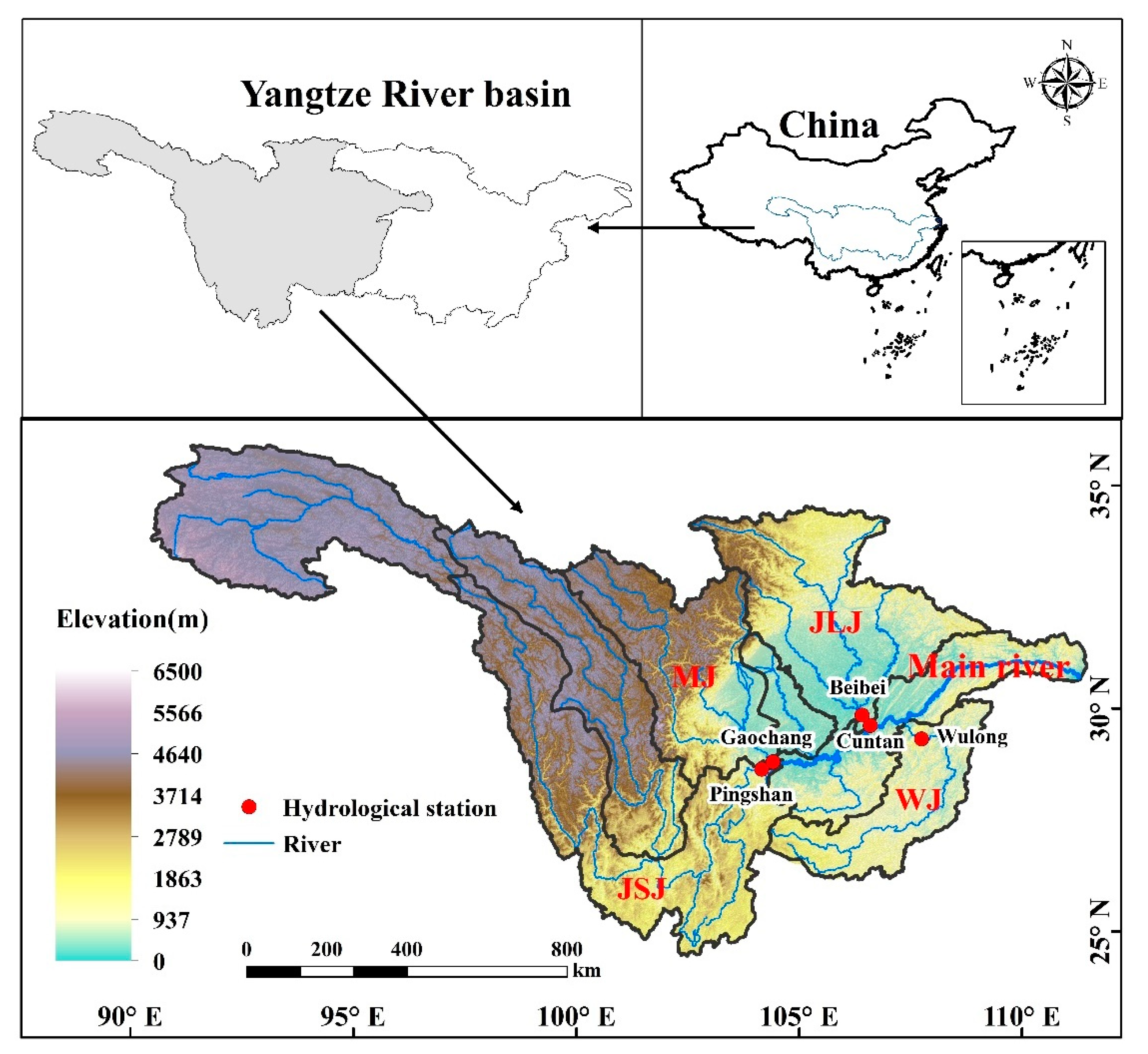
2.1. Study Area

The upper Yangtze River basin starts from the Kunlun Mountains at 4800 m in the west and extends 4500 km to Yichang City, Hubei Province, controlling an area of 1 million km2, which occupies over 60% of the Yangtze River (Figure 1). The elevation is approximately 200~6500 m, and the mountains and plateaus area occupies over 90% of the basin. The annual rainfall is about 1000~1400 mm, and the annual runoff is about 4.35 × 10¹¹ m3. Due to the influence of general circulation of atmosphere and terrain factors, the character of rainfall shows a decreasing trend from southeast to northwest in the upper Yangtze River basin, which may arise mountain torrents and soil erosion during the rainy season [42,43]. The major tributaries of the upper Yangtze River include Jinshajiang, Jialingjiang, Wujiang, Minjiang, etc. The runoff of the Jinshajiang occupies over 40% of the upper Yangtze River basin, which is the primary source of runoff of the Yangtze River.

2.2. Data Preprocessing

In this study, the mid- to long-term runoff prediction in the upper Yangtze River is conducted in five control gauges (Table 1), i.e., Pingshan, Beibei, Wulong, Gaochang, and Cuntan in the Jinshajiang, Jialingjiang, Wujiang, Minjiang, and the main river of the Yangtze River, respectively. The daily-observed discharge of hydrological stations from 1980 to 2018 were collected from the Changjiang Water Resources Commission of the Ministry of Water Resources and the hydrological statistical yearbook. Mid- to long-term runoff prediction requires preprocessing of the data at different time scales. Firstly, it is necessary to clarify the criteria for dividing ten-day and monthly scales data [44,45]. In the ten-day runoff prediction, the first ten days, the middle ten days, and the last part of each month as the basis for dividing the ten days. On the other hand, in the monthly runoff prediction, the data calculation is based on the actual number of days per month. Eventually, the daily runoff data are accumulated and averaged to obtain ten-day and monthly runoff data.

3. Methods

As an essential branch of machine learning, deep learning originates from comprehensive research on artificial neural networks. Deep learning discovers distributed feature representations of data by combining low-level features to form more abstract high-level representations. As a result, it builds end-to-end high-intelligence applications [46]. The essence of runoff prediction is the problem of predicting time-series data. Deep learning can effectively extract the changing relationship of massive historical runoff observation data. Then, the inner links behind the runoff data are deeply excavated, which is conducive to realizing long-period, high-accuracy runoff prediction. Recurrent neural network (RNN) takes sequence data as input, recurses in the evolutionary direction of the sequence, and connects all nodes (recurrent units) in a chain. It has a significant advantage in the nonlinear characteristics of runoff sequences for learning [47]. Currently, recurrent neural networks have been widely used in various time series prediction and natural language processing fields [48]. Compared to traditional runoff prediction methods, RNN methods can use multiple forms of time-series data and learn complex and intrinsic relationships in the time series rather than just mechanically targeting certain fixed factors. This study selected RNN and improved models based on RNN structure long–short-term memory (LSTM) and gated recurrent units (GRU) for mid- to long-term runoff prediction analysis in the upper Yangtze River.

3.1. Deep Learning Methodology for Mid- to Long-Term Runoff Prediction

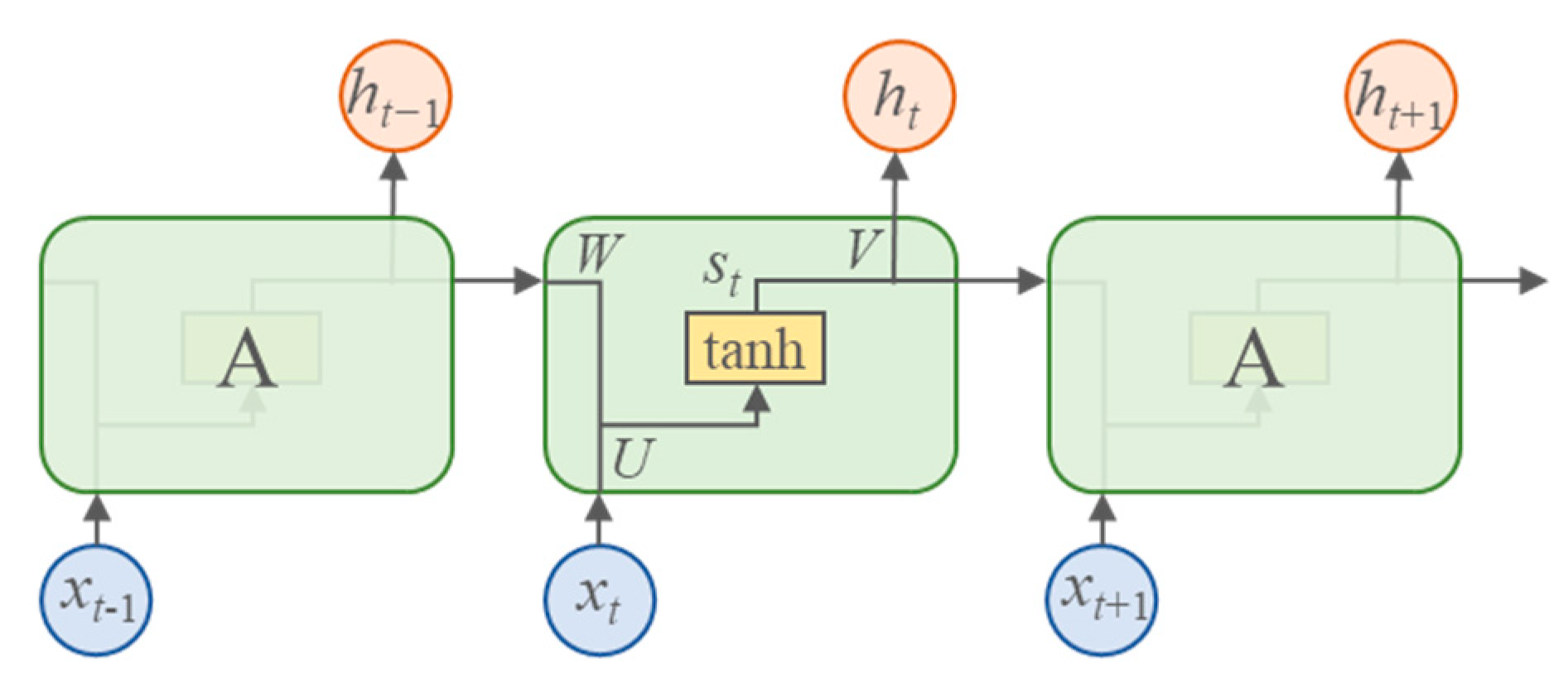
3.1.1. Recurrent Neural Network (RNN)

Recurrent neural network is a model with a short-term memory function to solve the problem of the continuity of training samples input sequence. In addition, the neurons in RNN can process information from other neurons while processing information from their neurons, thus forming a network structure with loop characteristics. The standard structure of RNN includes input units, hidden units, and output units [23]. RNN is a neural network with memory. When each hidden unit in the hidden layer produces output, it will consider memory, and with the next input, this hidden unit will not only consider the value of input but also consider the value in memory [49]. In general, RNN inputs { x o , x 1 , , x t , x t + 1 , } obtain hidden and output layers { h o , h 1 , , h t , h t + 1 , } . The structure of the GRU is as shown in Figure 2.
Where A represents the hidden unit, U , V , and W are the parameters of each remote unit; x t , h t , and s t , respectively, represent the input, output, and the state of the remote unit of the sample at the time. According to the network structure, it is well-known that all hidden layers of the RNN share the parameters of U , V , and W . The state s t is related to the current input conditions and the state s t 1 at the previous time. The relationship between them is as follows:
s t = tanh ( U · x t + W · s t 1 )
s t needs to be multiplied by the coefficient matrix V before output, and to the backpropagation of the error, the output result needs to be normalized and calculated to obtain the final result h t through the g function operation. The process of calculation is as follows:
h t = g ( V · s t )
g is the normalized exponential function softmax [50]. It is used as the activation function to simulate the neural stimulus. To ensure that there will be no output when the input is less than a certain value and that when the input is large enough, adding more inputs will not bring more sensitive results. The softmax function ensures that the probability of the predicted outcome is (0, 1), and the sum of probabilities is 1 [51]. The presence of a directed feedback mechanism in the implicit layer of the RNN allows the information from the last moment to act on the network state at the current moment. With self-feedback neurons, RNNs can process sequence data of arbitrary length. With the unknown parameters of U , V , and W , an update needs to be achieved by backpropagation. Each time the output value h t is compared with the actual value, it will generate an error value e t . The total error E can be calculated in Equation (3).
E = i = 0 t e i
RNN is a backpropagation model incorporating temporality. The computation from input to output can be achieved by resolving the values of parameters U , V and W according to the chain rule of derivation.

3.1.2. Long–Short-Term Memory (LSTM)

RNN can retain the information of the previous neurons, thereby establishing the dependency relationship between neurons. However, when the time lag is considerable, RNNs tend to lose this memorability and cannot continue to maintain the ability to learn information at a more extended time lag. Moreover, the RNN derivation process is prone to the vanishing gradient or the exploding gradient problems [39]. Therefore, RNN can only establish short-term dependencies, and it is difficult to establish long-term dependencies. To solve the above problems, LSTM is constructed based on RNN. As an improvement of RNN, LSTM introduces a gate mechanism in the circulation and loss of control features. As a result, LSTM can better solve the long-term dependencies of RNN. The gating unit of LSTM is mainly composed of three parts: input gate, forget gate, and output gate [52].
In LSTM, cells control memory content, the forgotten content, and how to use the gate to update the memory. The LSTM network structure is shown in Figure 3. It can be seen from the model structure that the transmission of data information between LSTM cells mainly depends on the transmission of cell state. The LSTM cell receives the input x t at the current moment, the cell state C t 1 , and the output data h t 1 at the last moment. Then, it completes the update of the current cell state C t and calculates the current output h t .
The forget gate of LSTM mainly determines the choice of information value. It receives the input x t at time t and output h t 1 at the last moment and outputs the forget gate result f t through σ (sigmoid function). The information transfer process is as follows [53]:
f t = σ ( W f · [ h t 1 , x t ] + b f )
where W f is the weight of the forget gate, and b f is the offset of the forget gate. At the same time, remove the value approaching 0 in the output of the forget gate and keep the value approaching 1.
The input gate of the LSTM consists of two parts, which are mainly responsible for deciding the useful memory information. The first part is to receive the input x t at time t and the output h t 1 at the previous time and input the gate result i t after processing by σ . The second part uses the tanh function to create a new candidate vector and add the vector C ˜ t to the cell state. The forward propagation process of the input gate is as follows:
i t = σ ( W i · [ h t 1 , x t ] + b i )
C ˜ t = tanh ( W c · [ h t 1 , x t ] + b c )
where W i is the input gate weight, b i is the input gate offset, W c is the candidate value weight, and b c is the candidate value offset. LSTM can use the past state C t 1 multiplied by the output f t of the forget gate to discard the information that needs to forget. The alternative value vector C ˜ t multiplied by the intermediate output i t can store the information that needs to be in memory. The process is as follows:
C t = f t C t 1 + i t C ˜ t
The output gate of LSTM is responsible for determining the output value, and Equation (8) can calculate the output gate calculation result vector o t at the output. W o is the weight of the output gate, and b o is the offset of the output gate.
o t = σ ( W o · [ h t 1 , x t ] + b o )
After activation of the cell state C t by the tanh function, the result h t is obtained according to Equation (9).
h t = o t tanh ( C t )

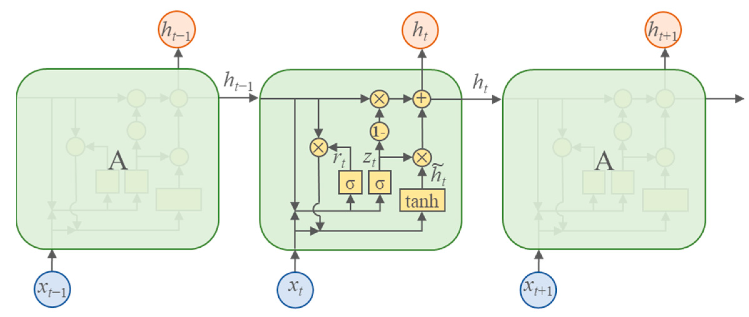
3.1.3. Gated Recurrent Unit (GRU)

GRU is a lightweight structure of LSTM [54]. In the structure of the GRU cell as shown in Figure 4.
The update gate corresponds to the input and forgets gate in LSTM. It controls the extent to which the state information from the previous moment is brought into the current state, which helps to capture the long-term dependence in the time series. The larger the update gate, the more state information is brought in at the last moment. The calculation process of the update gate is as follows:
z t = σ ( W z · [ h t 1 , x t ] )
where W z represents the weight, and z t represents the result of the update gate. The reset gate controls the state information of the last moment to be written into the current alternative hidden state h ˜ t to capture short-term dependencies in the time series. A smaller reset gate indicates that less state information has been written at the last moment. W r represents the weight of the reset gate. The process of resetting the gate output r t is as follows:
r t = σ ( W r · [ h t 1 , x t ] )
The calculation of the alternative hidden state h ˜ t at the current moment is as in Equation (11), where W h represents the weight of the candidate set.
h ˜ t = tanh ( W h · [ r t h t 1 , x t ] )
The output h t of the GRU unit is as follows:
h t = ( 1 z t ) h t 1 + z t h ˜ t
GRU uses a gating mechanism similar to LSTM to learn long-term dependencies. In addition, GRU simplifies the network structure of LSTM by designing only update and reset gates, reducing the number of connections and parameters, and optimizing the computational effort.

3.2. Model Calculation Schemes

This study aimed to explore the influence of time lag on the performance of RNN, LSTM, and GRU models at different time scales in mid- to long-term runoff prediction and determine the optimal time lag and lead time. Table 2 presents a total of 290 schemas that were developed for each RNN, LSTM, and GRU model. We used the sliding windows to generate the predicted sample at daily, ten-day, and monthly scales [37]. In addition, this study set 1980–2006 as the calibration period and 2007–2018 as the validation period.

3.3. Formatting of Mathematical Components

The performance of RNN, LSTM, and GRU models was evaluated with the Nash–Sutcliffe efficiency coefficient (NSE) and root mean square error (RMSE) [55] at multiple time scale runoff predictions in this paper. Generally, NSE is a common metric to quantify the prediction accuracy of hydrological simulations, and RMSE is used to compare the prediction results between different deep learning models [56,57]. NSE greater than 0.6 is an excellent prediction, between 0.4 and 0.6 is a reasonable prediction, and less than 0.4 is a poor prediction. The NSE and RMSE can be calculated as follows:
NSE = 1 i = 1 n ( Q c ( i ) Q O ( i ) ) 2 i = 1 n ( Q o ( i ) Q O ( i ) ¯ ) 2
RMSE = i = 1 n ( Q c ( i ) Q o ( i ) ) 2 n
where Q c and Q o are the predicted and observed discharge at the time i ; Q c ¯ and Q o ¯ are the average predicted and observed discharge; and n is the number of the datasets.

4. Results and Discussions

4.1. Daily Runoff Prediction

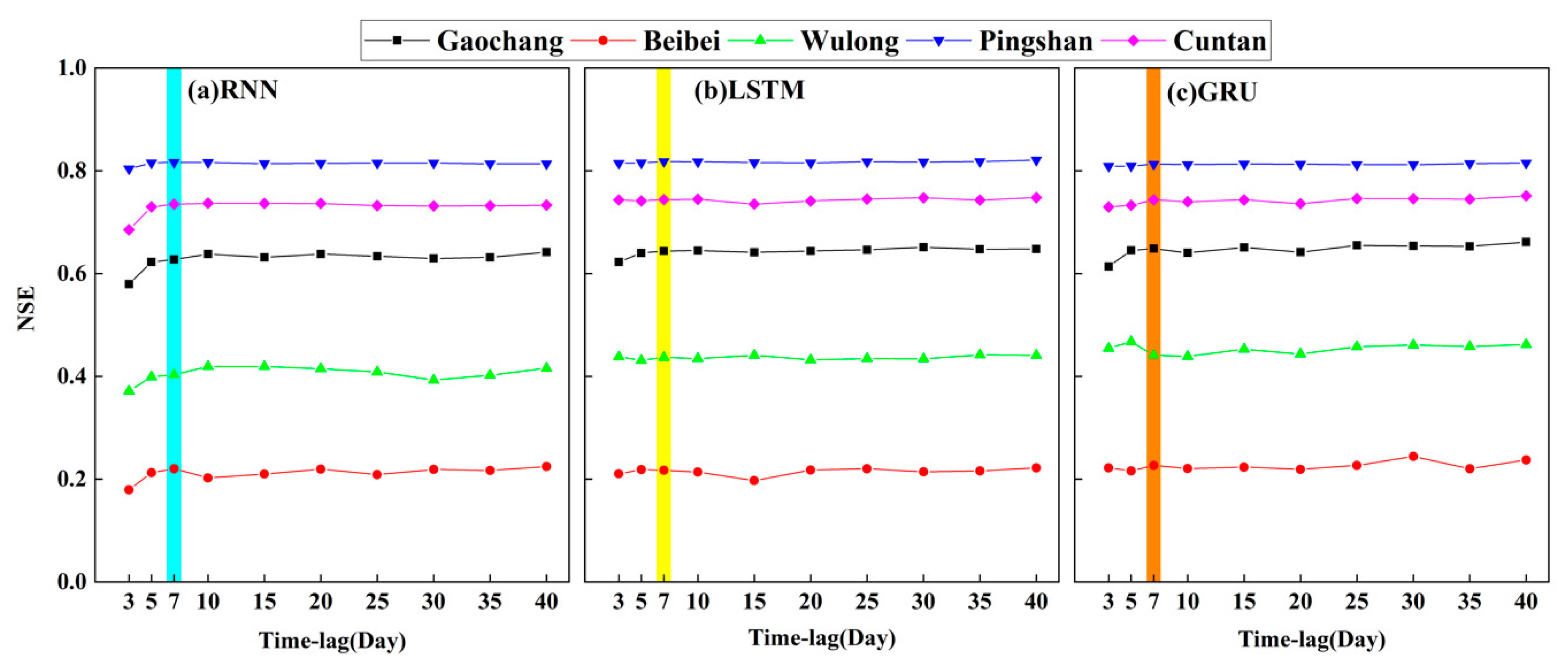
4.1.1. Performance Comparison among the RNN, LSTM, and GRU Models with Different Time Lags in Daily Runoff Prediction

The impact of the different time lags used in RNN, LSTM, and GRU models on daily runoff prediction results in Figure 5. The NSE of RNN, LSTM, and GRU models were gradually increased in short time lags. However, the number of time lags reached a particular value, which had a light effect. Therefore, choosing a specific value of time lags in results as an optimal parameter had greatly significant for daily runoff prediction. The optimal settings of the time lags at daily prediction were provided in Table 3. The optimal time lags of the three models were both 7 days, and the mean NSE were 0.560, 0.572, and 0.574. Overall, the varying time lags affected three models at daily runoff prediction.

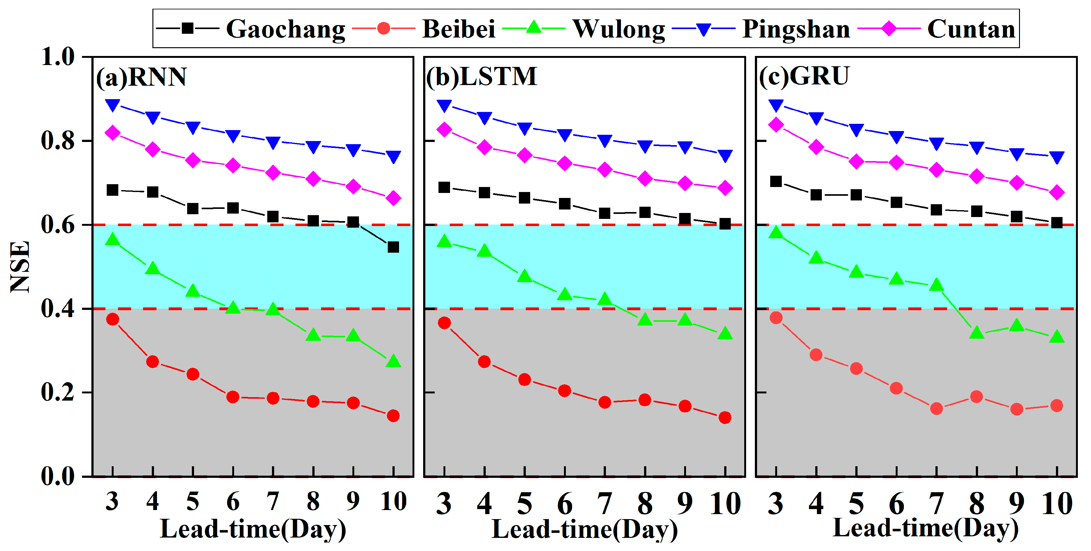
4.1.2. Multi-Day-Ahead Runoff Prediction

This section compared the different performances of the RNN, LSTM, and GRU models in multi-day ahead runoff prediction of optimal time-lags. Figure 6 shows the increase of lead time from 3 to 10 days had different influences in three models on the results of the runoff prediction. It can be seen that the accuracy of the three models gradually decreased with the increase of lead time.
As the lead time increased from 3 to 10 days, the predicted results for Pingshan and Cuntan were excellent. Likewise, the RNN model had excellent prediction results at Gaochang with lead time from 3 to 10 days, except for the performance of the RNN model, whose lead time equaled to 10 days. The prediction result of Wulong was reasonable when the lead time was less than or equal to 7 days. However, the prediction result was poor when the lead time was 8 to 10 days in Wulong. The overall prediction result for Beibei was poor. As a result, one day ahead was the best output in RNN, LSTM, and GRU at daily runoff prediction.

4.1.3. Modeling Parameter Optimization in Daily Runoff Prediction

This section compares the observed runoff processes with the simulated runoff processes in the RNN, LSTM, and GRU models when optimized time lag and lead time equaled 3 days. According to Table 4, the RMSE of the three models revealed that the RNN model was less effective than the LSTM and GRU models, but the result was not significant. Compared to the NSE of three models at each station, the best simulated Pingshan and the worst simulated Beibei were selected as the representatives for daily runoff prediction. Figure 7a,b, respectively, exhibits the Pingshan and Beibei predicted runoff processes in optimal time lag and lead time by three models. It can be observed that the performance of RNN, LSTM, and GRU were similar in daily runoff prediction when setting optimal parameters. Deep learning models successfully captured the runoff process in Pingshan and Beibei. However, it was hard to capture the high discharge in Beibei. Therefore, it could be demonstrated that RNN, LSTM, and GRU, although they had the reasonable capability in daily runoff prediction, still had significant shortcomings in predicting high discharge.

4.2. Ten-Day Runoff Prediction

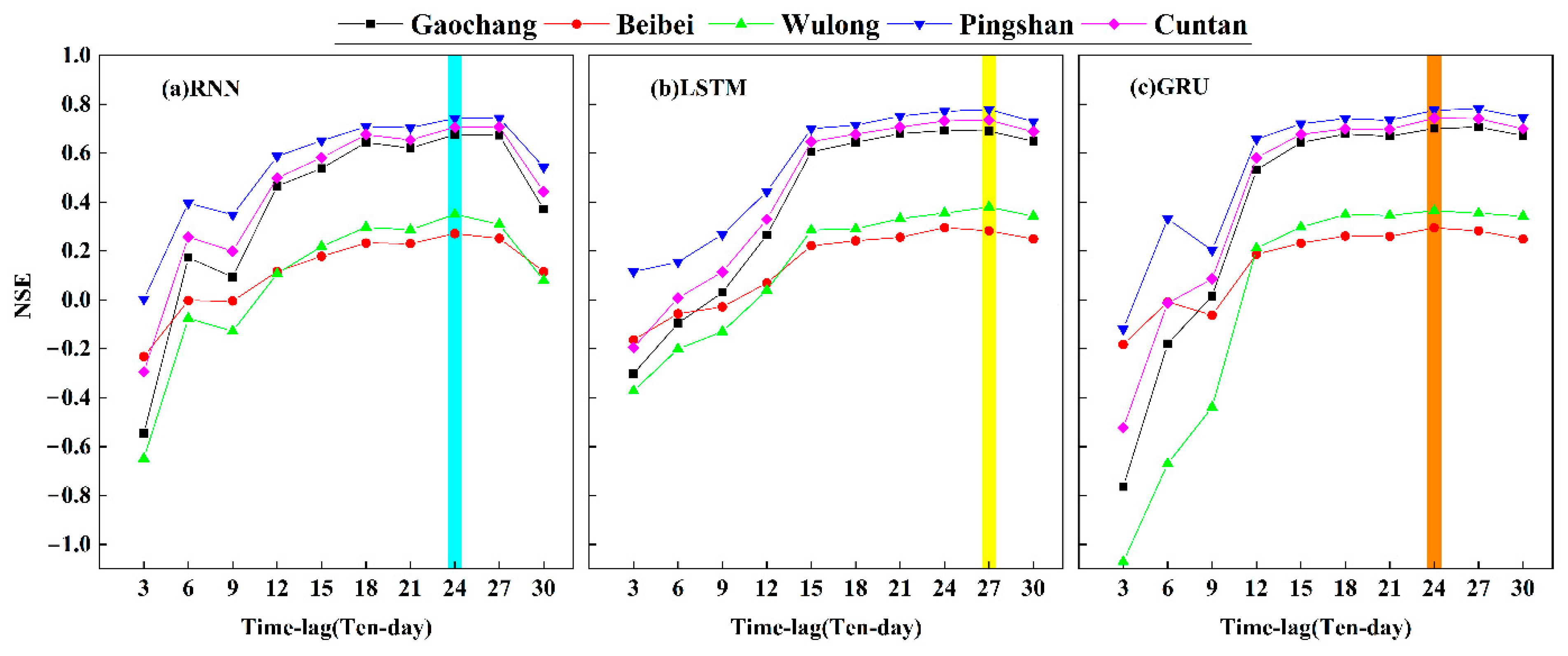
4.2.1. Performance Comparison among the RNN, LSTM, and GRU Models with Different Time Lags in Ten-Day Runoff Prediction

The performance of RNN, LSTM, and GRU for 10-day runoff prediction with different time lags is shown in Figure 8. It can be observed that variable time lags affected the NSE of the three models. NSE had a significant increase in the short time lags. In addition, there was only a slight variation of NSE when the time lag reached a specific value. Figure 8a–c, respectively, displays the slight NSE variation trend in the RNN, LSTM, and GRU models when the time lag begins with 12, 15, and 12 ten days. Significantly, the RNN model was different from other models. NSE had obvious change when time lag was equal to 30 ten days. The result of the runoff prediction may be affected by the exploding gradient in RNN [58]. The optimal time lags of the three models, and the mean NSE are shown in Table 5. The time lags of RNN, LSTM, and GRU, respectively, set to 24, 27, and 24 ten days would have the best results.

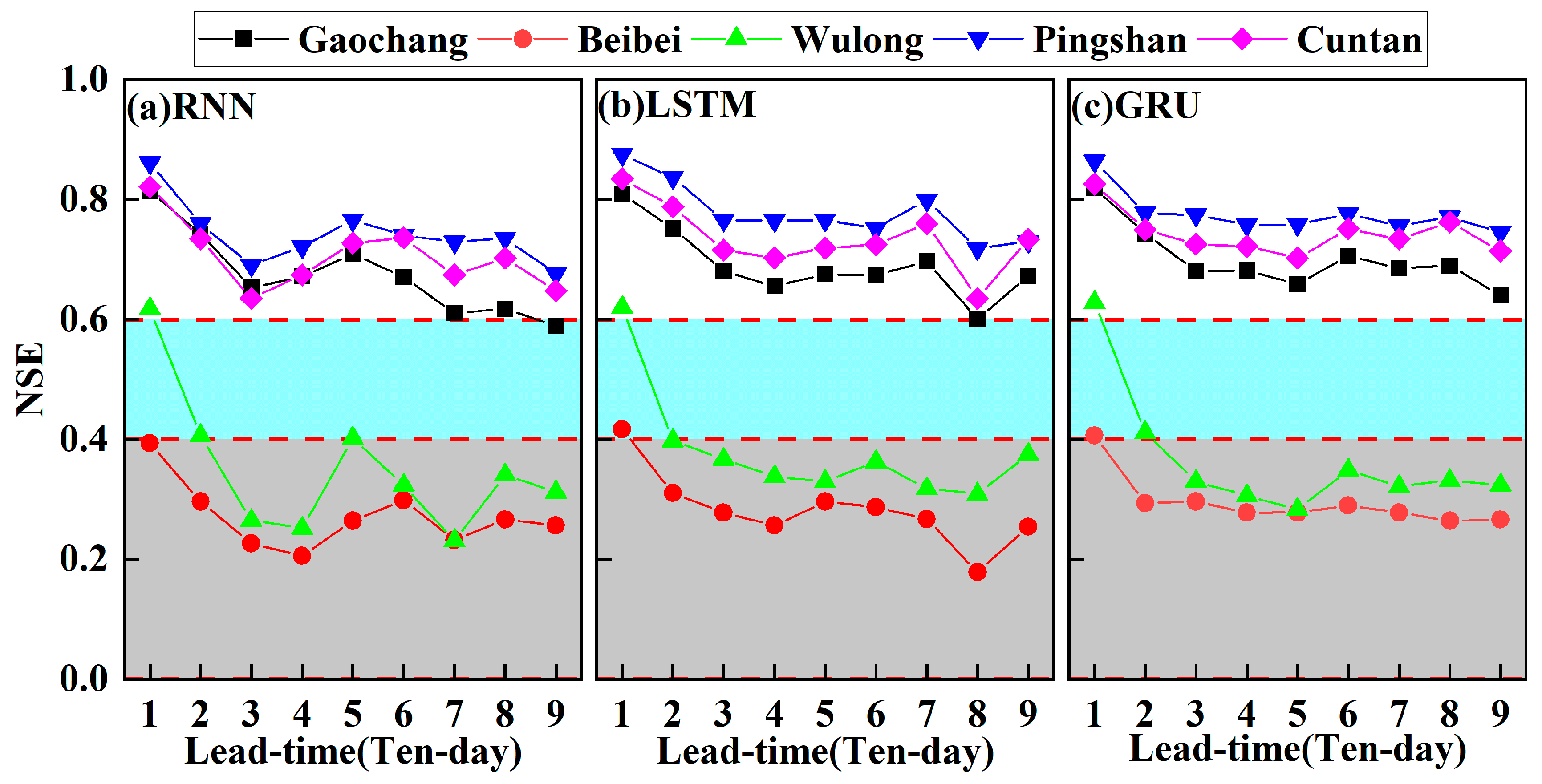
4.2.2. Multi-Ten-Day-Ahead Runoff Prediction

This section set lead time from 1–9 ten days in Figure 9 to compare the multi-ten-day-ahead runoff prediction in optimal time lags. The NSE of RNN, LSTM, and GRU models were fluctuant with the increase of the time lags, but it was easy to find the linear relation between them. Nevertheless, as the lead time increased from 1 ten day to 9 ten days, the prediction results for PingShan, Gaochang, and Cuntan were excellent. PingShan had excellent prediction results at lead time equaling 1 ten day and poor prediction results at the other lead time. The prediction results for Beibei were poor overall. In general, the predicted performance of each station was optimal at lead time of 1 ten day. Therefore, we could choose 1 ten days ahead as the best output in RNN, LSTM, and GRU at ten-day runoff prediction.

4.2.3. Modeling Parameter Optimization in Ten-Day Runoff Prediction

According to Table 6, the difference in RMSE of the three models was not significant, but the RMSE of RNN was always inferior to LSTM and GRU. Compared to the NSE of each station, the best simulated Pingshan and the worst simulated Beibei were selected as the representatives for ten-day runoff prediction. We compared the observed runoff processes with the RNN, LSTM, and GRU models when time lag and lead time were optimal in Pingshan and Beibei, as shown in Figure 10a,b. Although three models were well-simulated with observed discharge in Pingshan and Beibei, the result was similar to daily runoff prediction. It was hard to capture the high discharge in different years. The problem generally existed in the simulation of runoff prediction by deep learning models, for which the primary reason was underfitting [59]. As a result, we also needed to carefully consider the flood application at ten-day runoff prediction.

4.3. Monthly Runoff Prediction

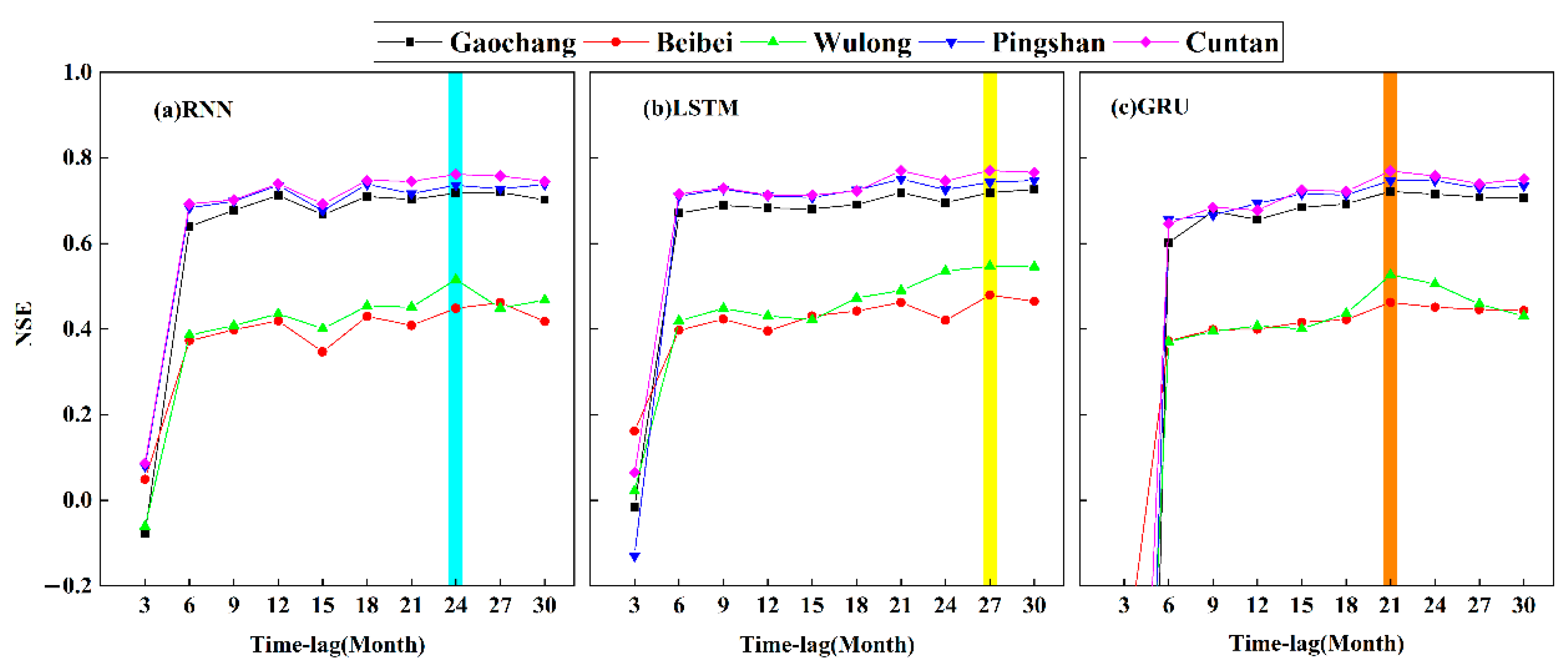
4.3.1. Performance Comparison among the RNN, LSTM, and GRU Models with Different Time Lags in Monthly Runoff Prediction

Figure 11 exhibits the performance of RNN, LSTM, and GRU at monthly runoff prediction. Again, it can be found that the three models had terrible performance when time-lag was equal to 3 months. In particular, the NSE of the GRU model was less than −0.2, which was the worst performance of the three models. According to Figure 11c, when the time lag was equal to 3 months, the NSE of Gaochang, Beibei, Wulong, Pingshan, and Cuntan were −3.5, −0.4, −1.8, −2.5, and −1.7, respectively. However, the variance of NSE was no longer an evident trend of fluctuation after the time lag of 6 months. As shown in Table 7, the optimal time lags of RNN, LSTM, and GRU were 24, 27, and 21 months, which means NSE was 0.636, 0.652, and 0.646.

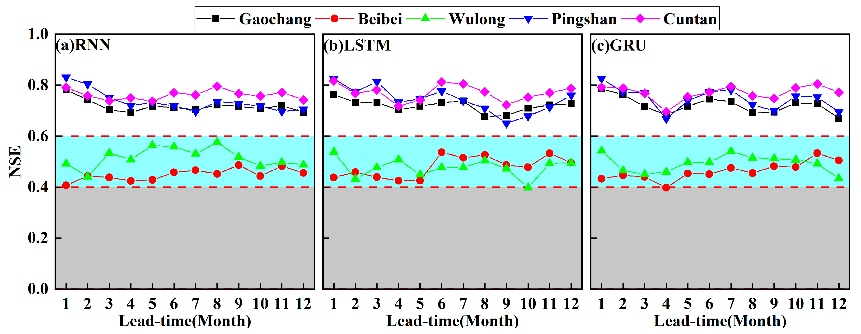
4.3.2. Multi-Month-Ahead Runoff Prediction

Figure 12 shows the NSE of RNN, LSTM, and GRU models in the optimal monthly time lags when setting the lead time from 1 to 12 months. Again, the predicted performance of PingShan, Cuntan, and Gaochang was all excellent. Likewise, the predicted performance of Beibei and Wulong was all reasonable. Moreover, it revealed that the NSE of the three models had no significant change with the increase of lead times at monthly runoff prediction. One month ahead was the best output for Pingshan, Cuntan, and Gaochang. Except for the output of RNN for Wulong, the one-month output of LSTM and GRU were the best. Except for the RNN prediction results, the results of LSTM and GRU were all best in one-month-ahead prediction for Wulong. Although the best output of Beibei was not one month ahead, the difference between the NSE of one month ahead and the best NSE in RNN, LSTM, and GRU was 16.1%, 17.7%, and 18.8%, respectively, which was not significant. Therefore, according to the above analysis, we suggest that one month ahead can be the best output at monthly runoff prediction.

4.3.3. Modeling Parameter Optimization in Monthly Runoff Prediction

According to Table 8, the RMSE of RNN was greater than LSTM and GRU at monthly runoff prediction. Compared to the NSE of each station, the best simulated Pingshan and the worst simulated Beibei were selected as the representatives for monthly runoff prediction. We set the optimal time lag and lead time to compare the observed with the predicted discharge from RNN, LSTM, and GRU models in Pingshan and Beibei. As shown in Figure 13, the NSE of the three models was higher than 0.8 in Pingshan and was higher than 0.4 in Beibei, for which the result of simulations can reach the requirement of runoff prediction. However, the problem of monthly runoff prediction was similar to daily and ten-day runoff prediction. For example, three models were hard to capture the high discharge at monthly runoff prediction, and it was also hard to capture low discharge. In addition, the underfitting effect of deep learning was prominent at monthly runoff prediction. Generally, RNN, LSTM, and GRU models could predict the process of monthly runoff. However, applying RNN, LSTM, and GRU in monthly runoff prediction was insufficient when faced with extreme runoff events.

4.4. Comparison of the Runoff Prediction at Different Time Scales

To analyze the parameters of RNN, LSTM, and GRU models that affected the result of runoff prediction, it was significant to divide into the time series of runoff by daily, ten-day, and monthly scales. The essence of deep learning model runoff prediction was a time-series prediction problem that took a series of past runoff data as input and a fixed-length runoff data series as output; therefore, time lags and lead times as important parameters had different effects at multiple time scales of runoff prediction [60]. Based on the previous analysis, we found that the increase of time lag would reduce the effect on NSE after time lag reached a specific value at different time scales. The above results corresponded with Gao et al. [37] finding the regularity of the short-term runoff prediction by GRU and LSTM. Besides, increased lead time was linearly related to decreased NSE at daily and ten-day runoff prediction. The increased lead time was poorly correlated with the input time lag in runoff prediction on daily and ten day, which may result in the loss of prediction accuracy, and this research result was consistent with the results of flood prediction by Hu et al. [61]. There was no significant linear relationship between NSE and lead time at monthly runoff predictions, but the lead-time length also had a slight effect on the final prediction results. Therefore, the lead-time length also played an influential role in different time scales: daily, ten day, and monthly. Overall, the setting of time lag and the output of lead time in the deep learning model is very important to the accuracy of runoff prediction results. As a result, the runoff’s time-series scale should be considered when we estimate the influence of time lags. In addition, we chose the exact lead times to obtain the best results at different time scales of runoff prediction [62].
Comparing Figure 6, Figure 9 and Figure 12, we found that the effect of lead time on the prediction results would decrease as the time scale increased. The possible reason for this phenomenon was the upscaling of the daily runoff data through our preprocessing, which had generalized the noise information in the data, resulting in less information for the deep learning model to learn, thus reducing the impact on the output results [63,64]. Moreover, Figure 7, Figure 10 and Figure 13 indicate that it is necessary to improve the simulation accuracy of extreme hydrological events in daily, ten-day, and monthly runoff prediction [65]. As a result, RNN, LSTM, and GRU are generally applicable for runoff prediction at different time scales at most stations.
This study presented that the simulation accuracy differed between stations. The deep learning model more greatly outperformed runoff predictions in PingShan, Cuntan, and Gaochang than in Beibei and Wulong. A possible cause of this phenomenon was the influence of human activity on runoff processes. The key to runoff prediction deep learning models was finding the data’s regulation [66]. However, the Jialingjiang basin controlled by Beibei Station and the Wujiang basin controlled by Wulong Station were the main areas of human activity in the upper Yangtze River basin [67]. The cascaded reservoirs interfered with the runoff process in the basin [68,69]. As a result, the deep learning model was affected to some extent in the learning process, making it challenging to find regulation between the data.
In addition, the simulation of runoff processes at different stations was affected by multiple factors, such as climate and human activity [70]. However, this paper focused on the effects of time lag and lead time on the prediction results of RNN, LSTM, and GRU models at multiple time scales. The increased influence factors would improve the uncertainty of results. Therefore, we only considered the observed and simulated discharge of stations. In the subsequent study, we will try to introduce upstream station discharge and atmospheric circulation factors to evaluate the influence of different factors on runoff prediction [71].

5. Conclusions

This paper divided the runoff time series by daily, ten-day, and monthly scales to explore the performance of RNN, LSTM, and GRU models by various time lag and lead time. The three models were applied to the upper Yangtze River. Some important conclusions can be summarized as:
(1)
In daily runoff prediction, the optimal time lag was 7 days, and the optimal lead time was 3 days in RNN, LSTM, and RNN models. The prediction process of runoff achieved a good relationship with observation in optimal parameters settings. However, the models still had significant shortcomings in predicting high discharge.
(2)
In ten-day runoff prediction, the time lags of RNN, LSTM, and GRU models, respectively, were set to 24, 27, and 24 ten-days, and we set the lead time of 1 ten day as that which would have the best results. However, the three models proved hard to capture the high discharge at the process of ten-day runoff.
(3)
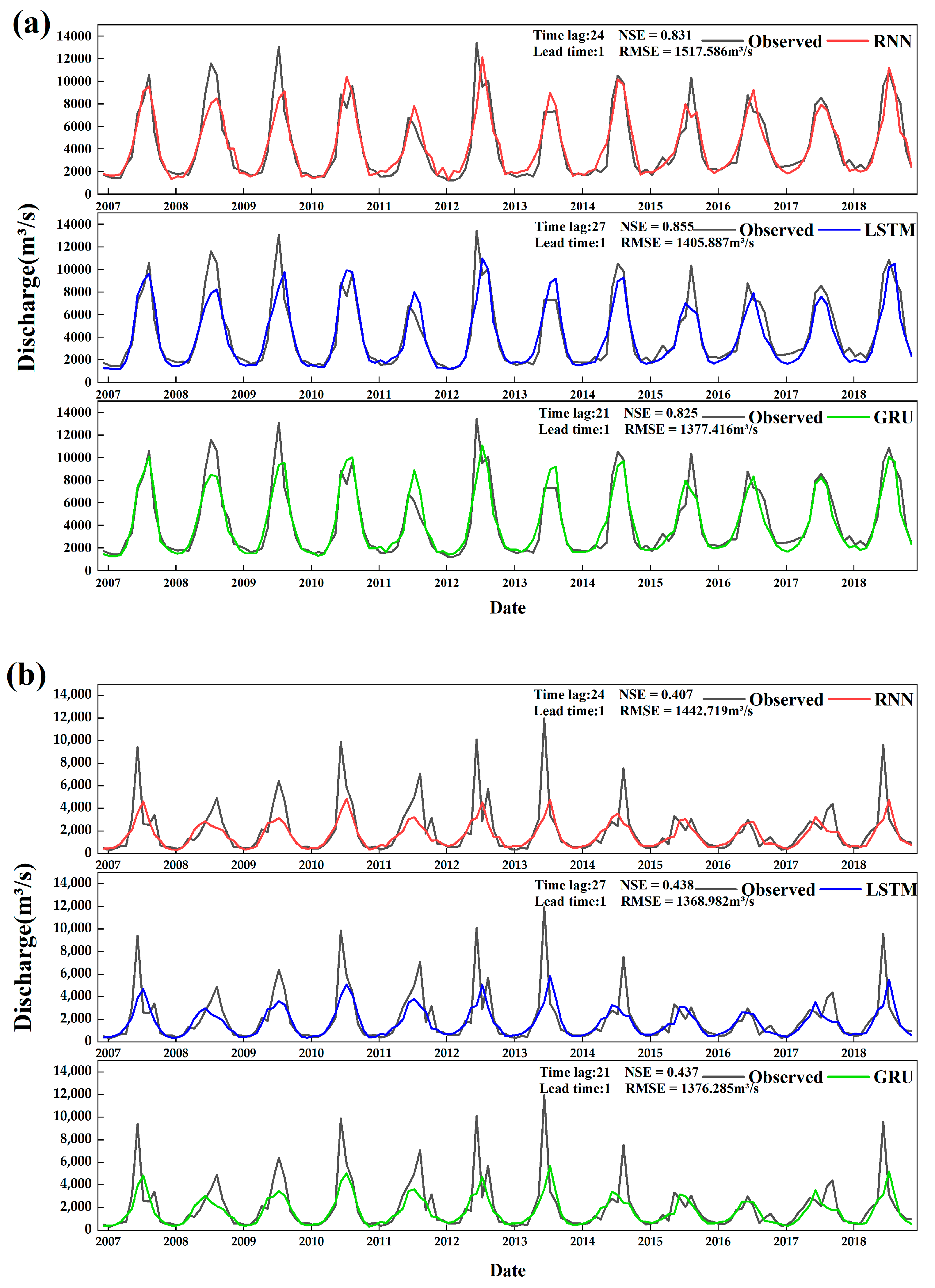
In monthly runoff prediction, the optimal time-lags were 24, 27, and 21 months, and optimal lead time was 1 month of RNN, LSTM, and GRU models. Although the three models were well-simulated with observed discharge at monthly runoff prediction, it was hard to accurately capture the low and high discharge.
(4)
The length of time lag and the lead time greatly impacted the results of RNN, LSTM, and GRU models at daily, ten-day, monthly runoff prediction. With the increase of time lags, the simulation accuracy stabilized after a specific time lag at multiple time scales of runoff prediction. Increased lead time was linearly related to decreased NSE at daily and ten-day runoff prediction. However, there was no significant linear relationship between NSE and lead time at monthly runoff prediction. The RMSE of the three models revealed that RNN was inferior to LSTM and GRU in runoff prediction. In addition, RNN, LSTM, and GRU models could not accurately predict extreme runoff events at different time scales.

Author Contributions

Formal analysis and writing—original draft, Y.R.; methodology, conceptualization, writing—review and editing, S.Z.; investigation, J.L.; data analysis, Z.T. and X.H.; methodology, Z.L.; conceptualization, J.S. and J.X. All authors have read and agreed to the published version of the manuscript.

Funding

This research was funded by the Hubei Key Laboratory of Intelligent Yangtze and Hydroelectric Science Foundation (ZH20020001), the Strategic Priority Research Program of the Chinese Academy of Sciences (Grant No. XDA23040500), and the Youth Innovation Promotion Association, CAS (No.2021385), and the Central Guidance on Local Science and Technology Development Fund of Chongqing City (No.2021000069).

Institutional Review Board Statement

Not applicable.

Informed Consent Statement

Not applicable.

Data Availability Statement

The datasets used or analyzed during the current study are available from the corresponding author on reasonable request.

Acknowledgments

We thank anonymous reviewers for their valuable comments to improve the manuscript.

Conflicts of Interest

The authors declare no conflict of interest.

References

  1. Mosavi, A.; Ozturk, P.; Chau, K. Flood prediction using machine learning models: Literature review. Water 2018, 10, 1536. [Google Scholar] [CrossRef] [Green Version]
  2. You, G.J.; Thum, B.; Lin, F. The examination of reproducibility in hydro-ecological characteristics by daily synthetic flow models. J. Hydrol. 2014, 511, 904–919. [Google Scholar] [CrossRef]
  3. Bai, H.; Li, G.; Liu, C.; Li, B.; Zhang, Z.; Qin, H. Hydrological probabilistic forecasting based on deep learning and Bayesian optimization algorithm. Hydrol. Res. 2021, 52, 927–943. [Google Scholar] [CrossRef]
  4. Fang, Y.; Zhang, X.; Corbari, C.; Mancini, M.; Niu, G.; Zeng, W. Improving the Xin’anjiang hydrological model based on mass–energy balance. Hydrol. Earth Syst. Sci. 2017, 21, 3359–3375. [Google Scholar] [CrossRef] [Green Version]
  5. Gautam, S.; Costello, C.; Baffaut, C.; Thompson, A.; Svoma, B.; Phung, Q.; Sadler, E. Assessing Long-Term hydrological impact of climate change using an ensemble approach and comparison with global gridded Model-A case study on good Water creek experimental Watershed. Water 2018, 10, 564. [Google Scholar] [CrossRef] [Green Version]
  6. Troin, M.; Arsenault, R.; Wood, A.W.; Brissette, F.; Martel, J.L. Generating ensemble streamflow forecasts: A review of methods and approaches over the past 40 years. Water Resour. Res. 2021, 57, e2020WR028392. [Google Scholar] [CrossRef]
  7. Graeff, T.; Zehe, E.; Blume, T.; Francke, T.; Schröder, B. Predicting event response in a nested catchment with generalized linear models and a distributed Watershed model. Hydrol. Process 2012, 26, 3749–3769. [Google Scholar] [CrossRef]
  8. Valizadeh, N.; Mirzaei, M.; Allawi, M.F.; Afan, H.A.; Mohd, N.S.; Hussain, A.; El-Shafie, A. Artificial intelligence and geostatistical models for stream-flow forecasting in ungauged stations: State of the art. Nat. Hazards 2017, 86, 1377–1392. [Google Scholar] [CrossRef]
  9. Gao, Y.; Yuan, Y.; Wang, H.; Schmidt, A.R.; Wang, K.; Ye, L. Examining the effects of urban agglomeration polders on flood events in Qinhuai River basin, China with HEC-HMS model. Water Sci. Technol. 2017, 75, 2130–2138. [Google Scholar] [CrossRef]
  10. Chen, Y.; Gao, J.; Bin, Z.; Qian, J.; Pei, R.; Zhu, H. Application study of IFAS and LSTM models on runoff simulation and flood prediction in the Tokachi River basin. J. Hydroinform. 2021, 23, 1098–1111. [Google Scholar] [CrossRef]
  11. Rujner, H.; Leonhardt, G.; Marsalek, J.; Viklander, M. High-resolution modelling of the grass swale response to runoff inflows with Mike SHE. J. Hydrol. 2018, 562, 411–422. [Google Scholar] [CrossRef]
  12. Li, C.; Zhu, L.; He, Z.; Gao, H.; Yang, Y.; Yao, D.; Qu, X. Runoff Prediction Method Based on Adaptive Elman Neural Network. Water 2019, 11, 1113. [Google Scholar] [CrossRef] [Green Version]
  13. Kan, G.; Yao, C.; Li, Q.; Li, Z.; Yu, Z.; Liu, Z.; Ding, L.; He, X.; Liang, K. Improving event-based rainfall-runoff simulation using an ensemble artificial neural network based hybrid data-driven model. Stoch. Environ. Res. Risk. A 2015, 29, 1345–1370. [Google Scholar] [CrossRef]
  14. Amin, S.; Van Moer, W.; Handel, P.; Ronnow, D. Characterization of concurrent Dual-Band power amplifiers using a dual Two-Tone excitation signal. IEEE T. Instrum. Meas. 2015, 64, 2781–2791. [Google Scholar] [CrossRef]
  15. Elshorbagy, A.; Corzo, G.; Srinivasulu, S.; Solomatine, D.P. Experimental investigation of the predictive capabilities of data driven modeling techniques in hydrology-Part 2: Application. Hydrol. Earth. Syst. Sci. 2010, 14, 1943–1961. [Google Scholar] [CrossRef] [Green Version]
  16. Muñoz, P.; Orellana-Alvear, J.; Willems, P.; Célleri, R. Flash-Flood forecasting in an andean mountain catchment—Development of a Step-Wise methodology based on the random forest algorithm. Water 2018, 10, 1519. [Google Scholar] [CrossRef] [Green Version]
  17. Li, Z.; Kang, L.; Zhou, L.; Zhu, M. Deep learning framework with time series analysis methods for runoff prediction. Water 2021, 13, 575. [Google Scholar] [CrossRef]
  18. Bergen, K.J.; Johnson, P.A.; de Hoop, M.V.; Beroza, G.C. Machine learning for data-driven discovery in solid Earth geoscience. Science 2019, 363, eaau0323. [Google Scholar] [CrossRef]
  19. Shi, B.; Hu, C.H.; Yu, X.H.; Hu, X.X. New fuzzy neural network-Markov model and application in mid-to long-term runoff forecast. Hydrol. Sci. J. 2016, 61, 1157–1169. [Google Scholar] [CrossRef] [Green Version]
  20. Sharafati, A.; Tafarojnoruz, A.; Shourian, M.; Yaseen, Z.M. Simulation of the depth scouring downstream sluice gate: The validation of newly developed data-intelligent models. J. Hydro-Environ. Res. 2020, 29, 20–30. [Google Scholar] [CrossRef]
  21. Li, H.; Tian, L.; Wu, Y.; Xie, M. Improvement of mid-to long-term runoff forecasting based on physical causes: Application in Nenjiang basin, China. Hydrol. Sci. J. 2013, 58, 1414–1422. [Google Scholar] [CrossRef] [Green Version]
  22. Chu, H.; Wei, J.; Li, T.; Jia, K. Application of support vector regression for mid-and long-term runoff forecasting in “yellow river headWater” region. Procedia Eng. 2016, 154, 1251–1257. [Google Scholar] [CrossRef] [Green Version]
  23. Zhang, J.; Chen, X.; Khan, A.; Zhang, Y.; Kuang, X.; Liang, X.; Taccari, M.L.; Nuttall, J. Daily runoff forecasting by deep recursive neural network. J. Hydrol. 2021, 596, 126067. [Google Scholar] [CrossRef]
  24. Wang, Q.; Huang, J.; Liu, R.; Men, C.; Guo, L.; Miao, Y.; Jiao, L.; Wang, Y.; Shoaib, M.; Xia, X. Sequence-based statistical downscaling and its application to hydrologic simulations based on machine learning and big data. J. Hydrol. 2020, 586, 124875. [Google Scholar] [CrossRef]
  25. Xie, K.; Liu, P.; Zhang, J.; Han, D.; Wang, G.; Shen, C. Physics-guided deep learning for rainfall-runoff modeling by considering extreme events and monotonic relationships. J. Hydrol. 2021, 603, 127043. [Google Scholar] [CrossRef]
  26. Mao, G.; Wang, M.; Liu, J.; Wang, Z.; Wang, K.; Meng, Y.; Zhong, R.; Wang, H.; Li, Y. Comprehensive comparison of artificial neural networks and long short-term memory networks for rainfall-runoff simulation. Phys. Chem. Earth Parts A/B/C 2021, 123, 103026. [Google Scholar] [CrossRef]
  27. Thapa, S.; Li, H.; Li, B.; Fu, D.; Shi, X.; Yabo, S.; Lu, L.; Qi, H.; Zhang, W. Impact of climate change on snowmelt runoff in a Himalayan basin, Nepal. Environ. Monit. Assess. 2021, 193, 1–17. [Google Scholar] [CrossRef]
  28. Zhang, D.; Peng, Q.; Lin, J.; Wang, D.; Liu, X.; Zhuang, J. Simulating reservoir operation using a recurrent neural network algorithm. Water 2019, 11, 865. [Google Scholar] [CrossRef] [Green Version]
  29. Moazami Goudarzi, F.; Sarraf, A.; Ahmadi, H. Prediction of runoff within Maharlu basin for future 60 years using RCP scenarios. Arab. J. Geosci. 2020, 13, 605. [Google Scholar] [CrossRef]
  30. Feng, Z.; Niu, W.; Tang, Z.; Jiang, Z.; Xu, Y.; Liu, Y.; Zhang, H. Monthly runoff time series prediction by variational mode decomposition and support vector machine based on quantum-behaved particle swarm optimization. J. Hydrol. 2020, 583, 124627. [Google Scholar] [CrossRef]
  31. Nonki, R.M.; Lenouo, A.; Tshimanga, R.M.; Donfack, F.C.; Tchawoua, C. Performance assessment and uncertainty prediction of a daily time-step HBV-Light rainfall-runoff model for the Upper Benue River Basin, Northern Cameroon. J. Hydrol. Reg. Stud. 2021, 36, 100849. [Google Scholar] [CrossRef]
  32. Li, Y.; Wei, J.; Wang, D.; Li, B.; Huang, H.; Xu, B.; Xu, Y. A medium and Long-Term runoff forecast method based on massive meteorological data and machine learning algorithms. Water 2021, 13, 1308. [Google Scholar] [CrossRef]
  33. Han, H.; Choi, C.; Jung, J.; Kim, H.S. Deep learning with long short term memory based Sequence-to-Sequence model for Rainfall-Runoff simulation. Water 2021, 13, 437. [Google Scholar] [CrossRef]
  34. Moghadam, S.V.; Sharafati, A.; Feizi, H.; Marjaie, S.M.S.; Asadollah, S.B.H.S.; Motta, D. An efficient strategy for predicting river dissolved oxygen concentration: Application of deep recurrent neural network model. Environ. Monit Assess. 2021, 193, 798. [Google Scholar] [CrossRef]
  35. Chen, X.; Huang, J.; Wang, S.; Zhou, G.; Gao, H.; Liu, M.; Yuan, Y.; Zheng, L.; Li, Q.; Qi, H. A new Rainfall-Runoff model using improved LSTM with attentive long and short Lag-Time. Water 2022, 14, 697. [Google Scholar] [CrossRef]
  36. Chen, X.; Huang, J.; Han, Z.; Gao, H.; Liu, M.; Li, Z.; Liu, X.; Li, Q.; Qi, H.; Huang, Y.; et al. The importance of short lag-time in the runoff forecasting model based on long short-term memory. J. Hydrol. 2020, 589, 125359. [Google Scholar] [CrossRef]
  37. Gao, S.; Huang, Y.; Zhang, S.; Han, J.; Wang, G.; Zhang, M.; Lin, Q. Short-term runoff prediction with GRU and LSTM networks without requiring time step optimization during sample generation. J. Hydrol. 2020, 589, 125188. [Google Scholar] [CrossRef]
  38. Yue, Z.; Ai, P.; Xiong, C.; Hong, M.; Song, Y. Mid-to long-term runoff prediction by combining the deep belief network and partial least-squares regression. J. Hydroinform. 2020, 22, 1283–1305. [Google Scholar] [CrossRef]
  39. Ji, Y.; Dong, H.; Xing, Z.; Sun, M.; Fu, Q.; Liu, D. Application of the decomposition-prediction-reconstruction framework to medium- and long-term runoff forecasting. Water Supply. 2021, 21, 696–709. [Google Scholar] [CrossRef]
  40. Zhao, X.; Lv, H.; Lv, S.; Sang, Y.; Wei, Y.; Zhu, X. Enhancing robustness of monthly streamflow forecasting model using gated recurrent unit based on improved grey wolf optimizer. J. Hydrol. 2021, 601, 126607. [Google Scholar] [CrossRef]
  41. Zhong, W.; Guo, J.; Chen, L.; Zhou, J.; Zhang, J.; Wang, D. Future hydropower generation prediction of large-scale reservoirs in the upper Yangtze River basin under climate change. J. Hydrol. 2020, 588, 125013. [Google Scholar] [CrossRef]
  42. Xiao, Z.; Shi, P.; Jiang, P.; Hu, J.; Qu, S.; Chen, X.; Chen, Y.; Dai, Y.; Wang, J. The spatiotemporal variations of runoff in the yangtze river basin under climate change. Adv. Meteorol. 2018, 2018, 5903451. [Google Scholar] [CrossRef] [Green Version]
  43. Su, B.; Huang, J.; Zeng, X.; Gao, C.; Jiang, T. Impacts of climate change on streamflow in the upper Yangtze River basin. Clim. Change 2017, 141, 533–546. [Google Scholar] [CrossRef]
  44. Wang, Z.; Qiu, J.; Li, F. Hybrid models combining EMD/EEMD and ARIMA for Long-Term streamflow forecasting. Water 2018, 10, 853. [Google Scholar] [CrossRef] [Green Version]
  45. Elganiny, M.A.; Eldwer, A.E. Enhancing the forecasting of monthly streamflow in the main key stations of the river Nile basin. Water Resour. Regime Water Bodies 2018, 5, 660–671. [Google Scholar] [CrossRef]
  46. LeCun, Y.; Bengio, Y.; Hinton, G. Deep learning. Nature 2015, 521, 436–444. [Google Scholar] [CrossRef]
  47. Zhou, J.; Zhang, Y.; Tian, S.; Lai, S. Forecasting Rainfall with Recurrent Neural Network for irrigation equipment. IOP conference series. Earth Environ. Sci. 2020, 510, 42040. [Google Scholar] [CrossRef]
  48. Nguyen, V.Q.; Anh, T.N.; Yang, H. Real-time event detection using recurrent neural network in social sensors. Int. J. Distrib. Sens. Netw. 2019, 15, 812338417. [Google Scholar] [CrossRef] [Green Version]
  49. Zhang, J.; Zhu, Y.; Zhang, X.; Ye, M. Yang J. Developing a Long Short-Term Memory (LSTM) based model for predicting water table depth in agricultural areas. J. Hydrol. 2018, 561, 918–929. [Google Scholar] [CrossRef]
  50. Ahmed, N.; Campbell, M. Variational bayesian learning of probabilistic discriminative models with latent softmax variables. IEEE Trans. Signal Processing 2011, 59, 3143–3154. [Google Scholar] [CrossRef]
  51. Totaro, S.; Hussain, A.; Scardapane, S. A non-parametric softmax for improving neural attention in time-series forecasting. Neurocomputing 2020, 381, 177–185. [Google Scholar] [CrossRef]
  52. Geng, Z.; Chen, G.; Han, Y.; Lu, G.; Li, F. Semantic relation extraction using sequential and tree-structured LSTM with attention. Inform. Sci. 2020, 509, 183–192. [Google Scholar] [CrossRef]
  53. Liu, X.; Zeng, Z.; Wunsch, D.C., II. Memristor-based LSTM network with in situ training and its applications. Neural Netw. 2020, 131, 300–311. [Google Scholar] [CrossRef] [PubMed]
  54. Ayzel, G.; Heistermann, M. The effect of calibration data length on the performance of a conceptual hydrological model versus LSTM and GRU: A case study for six basins from the CAMELS dataset. Comput. Geosci. 2021, 149, 104708. [Google Scholar] [CrossRef]
  55. Thapa, S.; Zhao, Z.; Li, B.; Lu, L.; Fu, D.; Shi, X.; Tang, B.; Qi, H. Snowmelt-Driven streamflow prediction using machine learning techniques (LSTM, NARX, GPR, and SVR). Water 2020, 12, 1734. [Google Scholar] [CrossRef]
  56. Sharafati, A.; Tafarojnoruz, A.; Motta, D.; Yaseen, Z.M. Application of nature-inspired optimization algorithms to ANFIS model to predict wave-induced scour depth around pipelines. J. Hydroinform. 2020, 22, 1425–1451. [Google Scholar] [CrossRef]
  57. Sharafati, A.; Tafarojnoruz, A. Yaseen Z M. New stochastic modeling strategy on the prediction enhancement of pier scour depth in cohesive bed materials. J. Hydroinform. 2020, 22, 457–472. [Google Scholar] [CrossRef]
  58. Ishida, K.; Kiyama, M.; Ercan, A.; Amagasaki, M.; Tu, T. Multi-time-scale input approaches for hourly-scale rainfall–runoff modeling based on recurrent neural networks. J. Hydroinform. 2021, 23, 1312–1324. [Google Scholar] [CrossRef]
  59. Li, W.; Kiaghadi, A.; Dawson, C. Exploring the best sequence LSTM modeling architecture for flood prediction. Neural Comput. Appl. 2021, 33, 5571–5580. [Google Scholar] [CrossRef]
  60. Cheng, M.; Fang, F.; Kinouchi, T.; Navon, I.M.; Pain, C.C. Long lead-time daily and monthly streamflow forecasting using machine learning methods. J. Hydrol. 2020, 590, 125376. [Google Scholar] [CrossRef]
  61. Hu, C.; Wu, Q.; Li, H.; Jian, S.; Li, N.; Lou, Z. Deep learning with a long Short-Term memory networks approach for Rainfall-Runoff simulation. Water 2018, 10, 1543. [Google Scholar] [CrossRef] [Green Version]
  62. Callegari, M.; Mazzoli, P.; de Gregorio, L.; Notarnicola, C.; Pasolli, L.; Petitta, M.; Pistocchi, A. Seasonal river discharge forecasting using support vector regression: A case study in the italian alps. Water 2015, 7, 2494–2515. [Google Scholar] [CrossRef] [Green Version]
  63. Wang, F.; Tian, D.; Lowe, L.; Kalin, L.; Lehrter, J. Deep learning for daily precipitation and temperature downscaling. Water Resour. Res. 2021, 57, e2020WR029308. [Google Scholar] [CrossRef]
  64. Baño-Medina, J.; Manzanas, R.; Gutiérrez, J.M. Configuration and intercomparison of deep learning neural models for statistical downscaling. Geosci. Model Dev. 2020, 13, 2109–2124. [Google Scholar] [CrossRef]
  65. Fang, W.; Xue, Q.; Shen, L.; Sheng, V.S. Survey on the application of deep learning in extreme weather prediction. Atmosphere 2021, 12, 661. [Google Scholar] [CrossRef]
  66. Liu, Y.; Zhang, T.; Kang, A.; Li, J.; Lei, X. Research on Runoff Simulations Using Deep-Learning Methods. Sustainability 2021, 13, 1336. [Google Scholar] [CrossRef]
  67. Liu, Y.; Xu, J.; Yao, L.; Guo, P.; Yuan, Z. The land use pattern and its changes in the upper reaches of the Yangtze River from 1980 to 2015. IOP conference series. Earth Environ. Sci. 2021, 676, 12097. [Google Scholar] [CrossRef]
  68. Zhang, J.; Zhang, M.; Song, Y.; Lai, Y. Hydrological simulation of the Jialing River Basin using the MIKE SHE model in changing climate. J. Water Clim. Change 2021, 12, 2495–2514. [Google Scholar] [CrossRef]
  69. Wu, X.; Xiang, X.; Chen, X.; Zhang, X.; Hua, W. Effects of cascade reservoir dams on the streamflow and sediment transport in the Wujiang River basin of the Yangtze River, China. Inland Waters Print 2018, 8, 216–228. [Google Scholar] [CrossRef]
  70. Li, S.; Xiong, L.; Li, H.; Leung, L.R.; Demissie, Y. Attributing runoff changes to climate variability and human activities: Uncertainty analysis using four monthly Water balance models. Stoch. Environ. Res. Risk A 2016, 30, 251–269. [Google Scholar] [CrossRef]
  71. Zhou, J.; Liu, Y.; Guo, H.; He, D. Combining the SWAT model with sequential uncertainty fitting algorithm for streamflow prediction and uncertainty analysis for the Lake Dianchi Basin, China. Hydrol. Process 2014, 28, 521–533. [Google Scholar] [CrossRef]
Figure 1. Major tributaries and hydrological stations located in the upper of the Yangtze River (JSJ, Jinshajiang; JLJ, Jialingjiang; WJ, Wujiang; MJ, Minjiang).
Water 14 01692 g001
Figure 2. RNN network structure.
Water 14 01692 g002
Figure 3. LSTM network structure.
Water 14 01692 g003
Figure 4. GRU network structure.
Water 14 01692 g004
Figure 5. NSE value of (a) RNN, (b) LSTM, and (c) GRU with different time lags (3, 5, 7, 10, 15, 20, 25, 30, 35, and 40 days) at daily prediction.
Water 14 01692 g005
Figure 6. The performance of runoff prediction at the lead times of 3–10 days by (a) RNN, (b) LSTM, and (c) GRU models with optimal time lags.
Water 14 01692 g006
Figure 7. Observed and predicted discharge from RNN, LSTM, and GRU models at optimal time lag and lead time at daily scale in (a) Pingshan and (b) Beibei.
Water 14 01692 g007
Figure 8. NSE value of (a) RNN, (b) LSTM, and (c) GRU with different time lags (3, 6, 9, 12, 15, 18, 21, 24, 27, and 30 ten days) at ten-day prediction.
Water 14 01692 g008
Figure 9. The performance of runoff prediction at the lead times of 1–9 ten days by (a) RNN, (b) LSTM, and (c) GRU models with optimal time lags.
Water 14 01692 g009
Figure 10. Observed and predicted discharge from RNN, LSTM, and GRU models at optimal time-lag and lead time at ten-day scale in (a) Pingshan and (b) Beibei.
Water 14 01692 g010
Figure 11. NSE value of (a) RNN, (b) LSTM, and (c) GRU with different time lags (3, 6, 9, 12, 15, 18, 21, 24, 27, and 30 months) at monthly prediction.
Water 14 01692 g011
Figure 12. The performance of runoff prediction at the lead times of 1–9 months by (a) RNN, (b) LSTM, and (c) GRU models with optimal time lags.
Water 14 01692 g012
Figure 13. Observed and predicted discharge from RNN, LSTM, and GRU models at optimal time lag and lead time at monthly scale in (a) Pingshan and (b) Beibei.
Water 14 01692 g013
Table 1. The information of five control gauges.
PingshanBeibeiWulongGaochang
Longitude104.16106.42107.75104.42
Latitude28.6329.8529.3228.8
Catchment area (km2)458,592156,14283,035135,378
Table 2. The time-lags and lead-times setting of models at daily, ten-day, and monthly scales.
ScaleParameter
DailyTime lag 35710152025303540
Lead time 345678910
Ten-dayTime lag 36912151821242730
Lead time 123456789
MonthlyTime lag 36912151821242730
Lead time123456789101112
Table 3. The optimal time-lag settings at daily prediction.
Time-Lag (Day)Mean NSE
RNN70.560
LSTM70.572
GRU70.574
Table 4. The performance of RNN, LSTM, and GRU models at daily runoff prediction with optimal time lag and lead time.
GaochangBeibeiWulongPingshanCuntan
NSERMSE
(m3/s)
NSERMSE
(m3/s)
NSERMSE
(m3/s)
NSERMSE
(m3/s)
NSERMSE
(m3/s)
RNN0.682 1277.144 0.374 2415.775 0.562 1153.855 0.888 1000.388 0.819 3468.217
LSTM0.689 1256.343 0.366 2408.034 0.558 1150.255 0.887 968.240 0.827 3348.614
GRU0.703 1238.188 0.378 2393.691 0.579 1126.187 0.888 967.555 0.839 3282.597
Table 5. The optimal time-lag settings at ten-day prediction.
Time Lag (Ten-Day)Mean NSE
RNN240.549
LSTM270.573
GRU240.576
Table 6. The performance of RNN, LSTM, and GRU models at ten-day runoff prediction with optimal time lag and lead time.
GaochangBeibeiWulongPingshanCuntan
NSERMSE
(m3/s)
NSERMSE
(m3/s)
NSERMSE
(m3/s)
NSERMSE
(m3/s)
NSERMSE
(m3/s)
RNN0.814 871.792 0.393 1784.135 0.617 930.174 0.861 1353.233 0.821 3183.543
LSTM0.809 819.733 0.417 1711.835 0.620 880.313 0.875 1306.992 0.834 3010.574
GRU0.819 841.442 0.415 1749.562 0.629 902.709 0.864 1299.684 0.826 3096.534
Table 7. The optimal time-lag settings at monthly prediction.
Time-Lag (Month)Mean NSE
RNN240.636
LSTM270.652
GRU210.646
Table 8. The performance of RNN, LSTM, and GRU models at monthly runoff prediction with optimal time lag and lead time.
GaochangBeibeiWulongPingshanCuntan
NSERMSE
(m3/s)
NSERMSE
(m3/s)
NSERMSE
(m3/s)
NSERMSE
(m3/s)
NSERMSE
(m3/s)
RNN0.782 723.898 0.407 1442.719 0.493 766.991 0.831 1517.586 0.791 3194.933
LSTM0.783 716.806 0.438 1368.982 0.538 734.883 0.855 1405.887 0.816 2998.444
GRU0.789 699.183 0.437 1376.285 0.587 739.440 0.825 1377.416 0.794 3022.717
Publisher’s Note: MDPI stays neutral with regard to jurisdictional claims in published maps and institutional affiliations.

