Assessment of the Potential of Coordinating Two Interacting Monitoring Networks within the Lerma-Santiago Hydrologic System in Mexico

Abstract

Water quality monitoring networks in the global south often display inefficiencies because monitoring strategies are frequently designed based on subjective professional judgments to define the temporal and spatial attributes of the networks, leading to poor cost–benefit relationships. The Lerma-Santiago Hydrological System (LSHS) in Mexico currently experiences severe environmental degradation caused by uncontrolled pollutant emissions from urban centers, agricultural, livestock, and industrial activities settled in the basin. While both the national and state authorities monitor this hydrological system, there has never been an effort to assess the monitoring efficiency of these two networks. The aim of the present study was to assess through multivariate statistical analyses the potential for coordination between these two interacting networks. For this purpose, two independent large water quality datasets with temporal and spatial attributes measured by two different authorities (the federal and the state) were used to identify those sites where coordination should be rationalized and those parameters that should continue to be monitored. The case study herein presented highlights the duplication in efforts to monitor surface water quality in the Lerma-Santiago hydrologic system, which implies a lack of coordination between the authorities and shows that water quality monitoring networks have not been reassessed since they were first implemented. Furthermore, using the case study of the Lerma-Santiago in Mexico, we expanded on various deficiencies, such as the use of different sampling frequencies and analytical methods by the authorities and inefficient communication among federal and state authorities. This study has revealed a large potential for coordinating two water quality monitoring networks (WQMN) in the Lerma-Santiago Hydrological System and a methodological approach that may be used to assess this potential. Coordination strategies for WQMNs can lead to significant cost reductions, extended network reach, and higher overall data quality in developing countries with limited financial resources and technical capabilities.

1. Introduction

1.1. Water Quality Monitoring in Developing Countries

Many developing countries are experiencing rapid urban development as well as agricultural and industrial growth. As a result, these countries are experiencing environmental degradation as they move along a path towards industrialization. Some of the main reasons for environmental damage in the global south is the inefficiency of governmental policies for environmental protection, limited financial, and technical resources to monitor resource usage and ecosystems health and their inability to act on the monitoring information when it is available [1].

The assessment of water resources requires a full comprehension of the processes affecting water quantity and quality. The establishment of water quality monitoring networks (WQMNs) involves the definition of the monitoring purpose and the desired information to be gathered, the monitoring network design (e.g., the temporal and spatial attributes), sampling or onsite measurement, laboratory analyses, data processing and verification, and data analysis. Such activities are performed to obtain information regarding the physical, chemical, and biological characteristics of water resources spatially distributed across a delimited region, usually hydrographic basins [2]. WQMNs help elucidate the various processes affecting water quality, allow the identification of problematic areas and the detection of both spatial and temporal trends, as well as providing water managers with the necessary information for water quality management. Moreover, these networks should fulfill these objectives in an accurate and efficient manner [2,3].

Surface water quality is strongly affected by point and nonpoint sources of anthropogenic pollution. Additionally, fast population growth and limited sanitation infrastructure exacerbate the presence of conflicts for water uses (e.g., irrigation, energy generation, public water supply, industry) [4]. Nevertheless, water quality monitoring in developing countries is often restricted by the availability of financial and technical resources. This hinders the effective development and use of WQMNs to provide policy makers with the information they need to make more informed decisions. Furthermore, WQMNs in developing countries often display inefficiencies such as monitoring redundancies because monitoring strategies are frequently designed based on subjective professional judgments to define the temporal and spatial attributes of WQMNs. Furthermore, once WQMMs are in use, they are rarely reassessed or readjusted, which leads to poor cost–benefit relationships [3]. Moreover, multiple authorities often overlap regarding their responsibilities for water management. As a result, there is often uncertainty in terms of which level of government is responsible for various aspects.

1.2. The Lerma-Santiago Hydrological System as a Case Study

Mexico is a clear example of a developing country experiencing rapid agro-industrial and urban growth. The impact of this growth can be observed in most waterbodies across the country and particularly in the lower Lerma and upper Santiago Hydrological System (LSHS), which comprises segments of the Lerma River, Zula River, Santiago River, and El Ahogado Stream, shown in Figure 1, and is known as the Santiago-Guadalajara basin. The LSHS experiences severe environmental degradation caused by intensive anthropogenic activities [5].

In Mexico, the water quality of surface water sources, coastal zones, and aquifers have been monitored through the federal WQMN of the National Commission of Water (CONAGUA) since 1996. By 2019, this network had 4655 sampling points across the country. Fifteen of these monitoring sites were established by CONAGUA within the LSHS in 2012 (Figure 1) [6]. Additionally, because the LSHS crosses the Mexican State of Jalisco, in 2009, the Jalisco State Water Commission (CEA) began to monitor periodically and to publish systematically the water quality data from the LSHS to evaluate the actions taken locally to mitigate the pollution in this hydrological system. The state WQMN now has 20 monitoring sites (Figure 1) [7]. As a result, both CONAGUA and CEA monitor LSHS sites close to each other [8]. There are likely some duplicated and possibly redundant efforts in monitoring the LSHS due to a lack of coordination between the federal and state entities, translating into the inefficient use of public resources for water management.

While both the national and local focus are important for the management of the LSHS at the river basin scale, there has never been an effort to assess the monitoring efficiency of these WQMNs collectively. Thus, there is a need to rationalize the two WQMNs by assessing the spatial distribution of the monitoring sites and the water quality parameters measured. Furthermore, the high costs associated with the WQMNs have been an obstacle to their expansion. The rationalization of these networks may reduce costs by eliminating less important water quality parameters and redundant monitoring sites [5,9].

1.3. Objective

The aim of the present study was to assess the rationalization potential of two interacting (joint) WQMNs in the LSHS basin administered by the federal and state authorities (CONAGUA and CEA), respectively, through multivariate statistical analyses. Two independent, large water quality datasets with temporal and spatial attributes measured by each authority were used to (i) identify the more relevant monitoring sites for possible prioritization and (ii) to identify the more relevant parameters that should continue to be monitored. In addition, those monitoring sites and water quality parameters that may be discontinued were identified.

Multivariate statistical techniques such as principal component analysis (PCA), cluster analysis (CA), discriminant analysis (DA), and principal factor analysis (PFA) have been used effectively for the assessment of WQMNs by various researchers in developing countries where monitoring strategies had been rarely reassessed or readjusted due to the lack of technical expertise [10]. For instance, Moura Calazans et al. [4] evaluated and proposed adjustments to the WQMN in the Paraopeba River basin (Brazil) comprised of 30 monitoring sites using multivariate statistical methods. Similarly, Moura Calazans et al. [10] conducted a WQMN optimization project for the WQMN for the Velhas River basin (Brazil) to identify the most relevant water quality parameters and monitoring sites. De Almeida et al. [3] assessed the São Paulo State (Brazil) WQMN to increase its spatial representativeness, as their analysis indicated monitoring site redundancy above 20%. Mavukkandy et al. [11] evaluated the monitoring efficiency of the WQMN in the Kabbini River basin of Kerala (India) and identified the insignificant monitoring sites in explaining the annual variance of the dataset. Peña-Guzmán et al. [12] proposed a redesign of the Tunjuelo River (Colombia) WQMN that would reduce the monitoring sites from nine to seven, which would reduce the sample acquisition and analysis costs across the network by 50%. Other approaches have been used for the rationalization of WQMNs. For instance, Mahjouri and Kerachian [13] evaluated and revised the spatial and temporal sampling frequencies of the water quality monitoring system of the Jajrood River in Tehran (Iran) using discrete entropy theory through a micro-genetic algorithm-based optimization model.

In the present study, PCA was initially applied to both water quality datasets to identify the key parameters to understand the variability in the water quality and to identify those that may be discontinued in favor of measuring other water quality parameters that are not currently measured. CA was used to identify the monitoring sites of both interacting WQMNs that respond similarly to the sources of pollution within the basin and that produce redundant information. DA was used to test the discriminating ability of the clusters previously identified by CA. These analyses were performed to determine the homogeneous groups of monitoring sites within the combined set of the monitoring sites belonging to both WQMNs (as a possible joint network) with a special focus on the comparison of neighboring monitoring sites to test for pairwise differences.

2. Materials and Methods

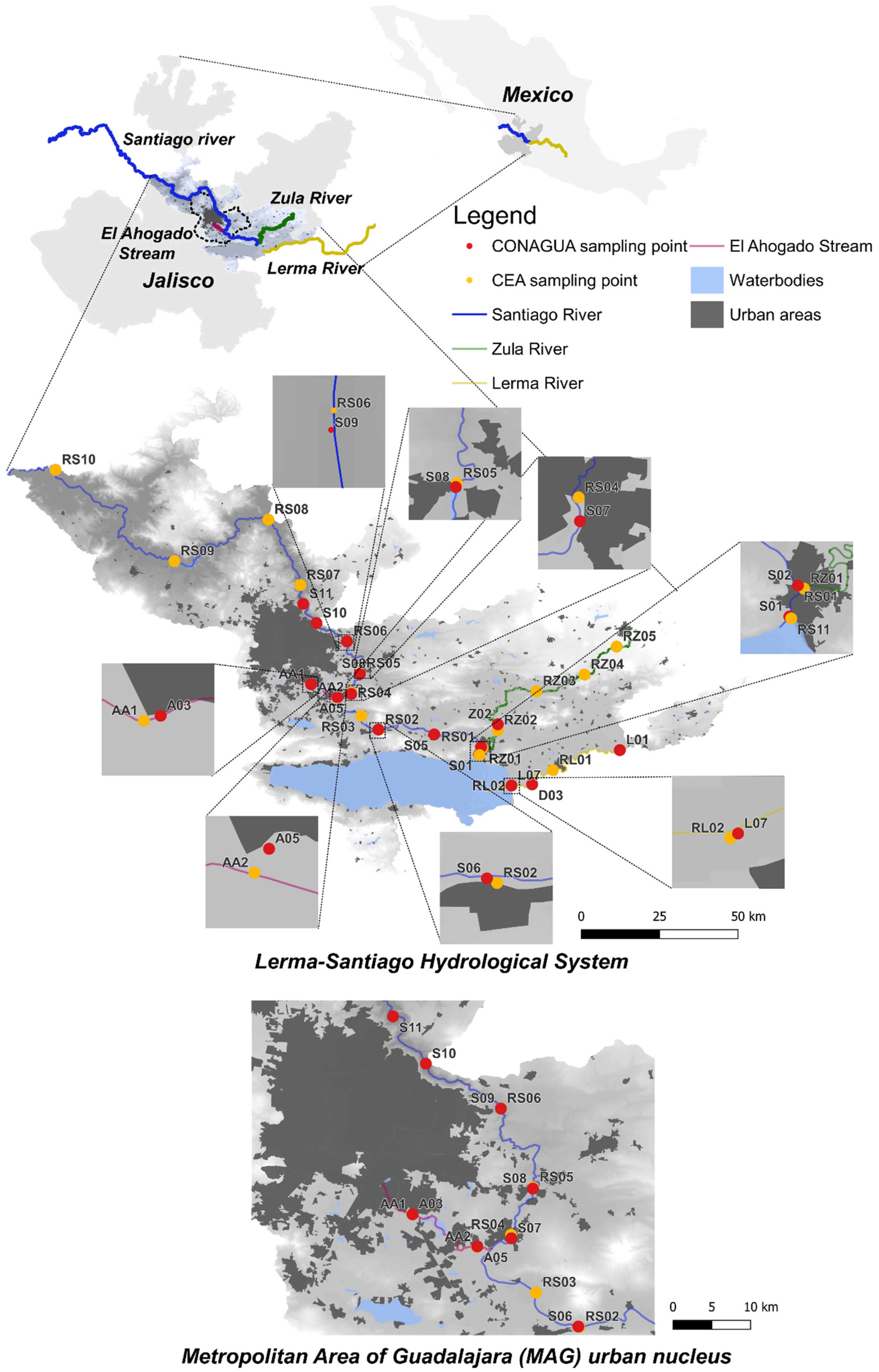
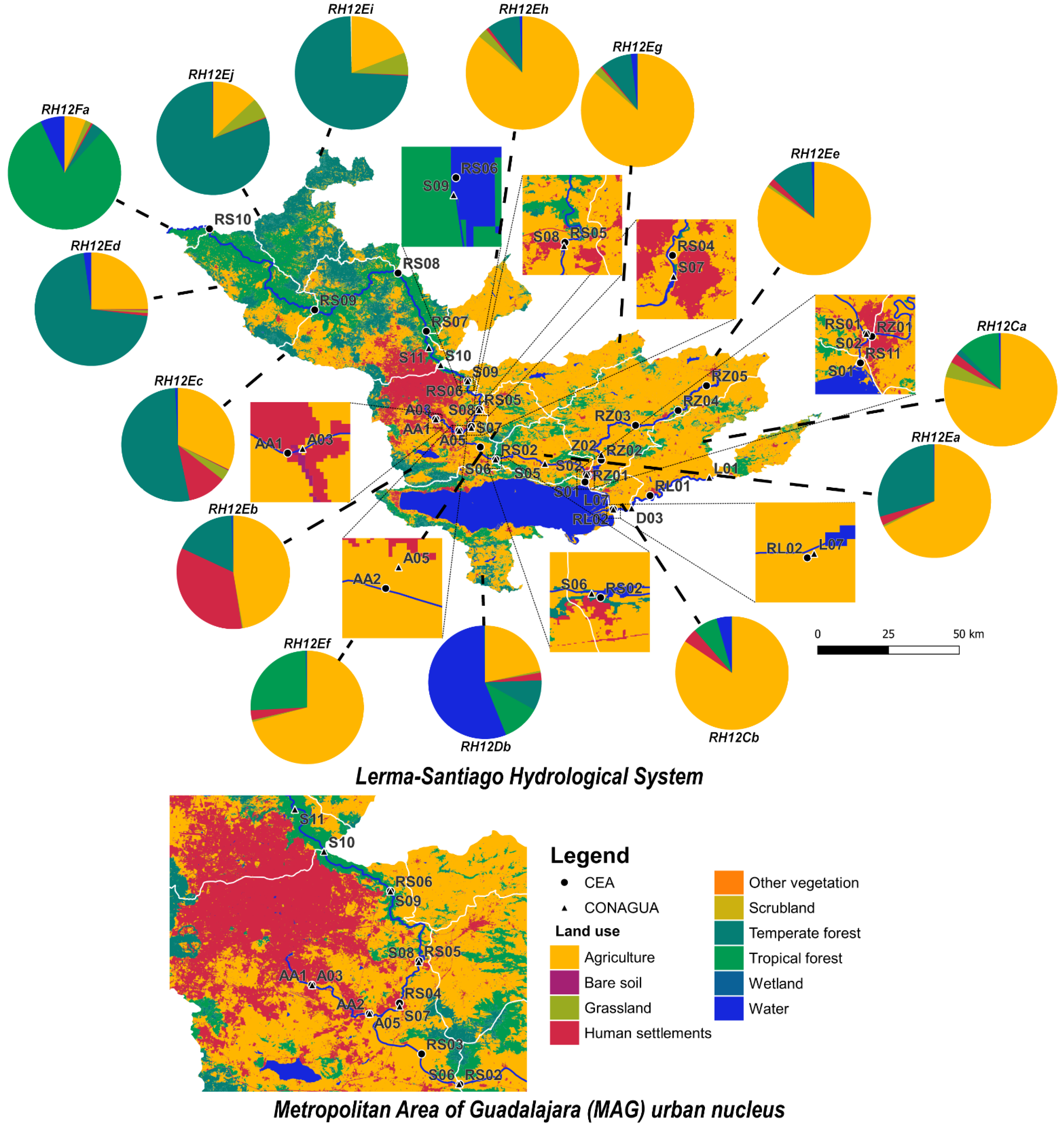
2.1. Study Area

The Lerma-Santiago hydrologic system (LSHS) herein studied consists of the Lerma-Chapala, the Santiago-Guadalajara, and the Zula basins. These three basins are comprised of fourteen sub-basins (see Figure 1). The Lerma River flows for 700 km from the state of Mexico to Lake Chapala in Jalisco state. The Santiago River flows for 433 km from Lake Chapala through the western section of the state of Jalisco, crossing the Guadalajara metropolitan area (GMA, the second largest metropolitan area in Mexico). The Santiago River then exits Jalisco and flows through the state of Nayarit and discharges to the Pacific Ocean (Figure 1). The Zula River and El Ahogado Stream are relevant tributaries to the Santiago River, flowing through agricultural and urban–industrial intensive regions, respectively [5,14,15]. The El Ahogado Stream receives significant loads of pollutants from partially treated or untreated urban wastewater from the El Ahogado WWTP, which is now over its treatment capacity by approximately 86,400 cubic meters/day (cmd). Additionally, the Agua Prieta WWTP, which discharges directly into Santiago River in the northern part of Guadalajara, is below its capacity by 172,800 cmd due to the lack of a wastewater collector tunnel section. The El Ahogado and Agua Prieta WWTPs receive approximately 20% and 80% of the GMA wastewater, respectively [5]. Although the GMA population of 5 million inhabitants is largely dependent on surface water from the Santiago-Guadalajara basin to meet its water demand [5,9], a large fraction of the industrial and urban wastewater generated within the basin is discharged without adequate treatment to the Santiago River or its tributaries [9].

The LSHS is widely known as the most polluted hydrological system in Mexico because of intense industrial activity, agricultural and livestock production, uncontrolled landfills and open dumps, and untreated urban wastewater discharges [5]. This multifactorial pollution problem has grown to be a significant public health concern, as the poor water quality within the basin has been correlated with health effects in population [16].

In the present study, we focused on the monitoring sites along the main channel of the Santiago River, as well as those located near the intersections of the Santiago River with the Lerma River, Lake Chapala, the Zula River, and the El Ahogado Stream (Figure 1). This study did not include those monitoring sites within Lake Chapala since they are only monitored by the federal authorities, and no rationalization was required.

The most recent land-use data (2018) for the LSHS was recovered from CONABIO [17] and reclassified according to Gebhardt et al. [18] reclassification methodology. Figure 2 shows that there are three main land-cover types in the basin: agriculture in the east, settlements in the central region, and forested land in the west. This figure allows clear identification of the distribution of land-cover types in each of the sub-basins.

2.2. The Water Quality Monitoring Networks and the Water Quality Data

As observed in Figure 1, the WQMN of CONAGUA within the LSHS is consists of 15 monitoring sites (red points), while the WQMN of CEA consists of 20 monitoring (yellow points), resulting in 35 monitoring sites managed by both authorities. These monitoring sites are distributed along the Lerma River (5 sites), the Zula River (6 sites), the Santiago River (20 sites), and the El Ahogado Stream (4 sites). CONAGUA and CEA have officially monitored 103 and 40 water quality parameters since 2012 and 2009, respectively [6,7]. However, the databases were not homogeneous (i.e., not all parameters were sampled at all monitoring sites and with the same sampling frequency in both datasets). Some parameters showed interruption of monitoring and changes in the sampling frequency. On average, CEA made 9.5 observations every year for each parameter at each sampling site, while the average for CONAGUA was 4.7 yearly observations made for each parameter at each monitoring site.

To select the parameters to be included in this study, the water quality parameter with the highest number of observations was identified and set to 100%. The number of observations for each remaining parameter was calculated as a percentage. Those parameters with a percentage of observations under 80% were excluded, as suggested by Sutadian et al. [19]. All water quality parameters included in this study and their abbreviations are presented in

Table 1. Water quality parameters included in this study.

Abbreviation	Parameter	Abbreviation	Parameter
Al	Aluminum	Ni	Nickel
ALKY	Alkalinity	NO2	Nitrite
As	Arsenic	NO3	Nitrate
Ba	Barium	ON	Organic nitrogen
BOD5	Biochemical oxygen demand	ORTO_PO4	Orthophosphates
BOD5_SOL	Soluble biochemical oxygen demand	Pb	Lead
Cd	Cadmium	pH	Hydrogen potential
CN-	Cyanide	Sulfide	Sulfur
COD	Chemical oxygen demand	SO4	Sulfates
COD_SOL	Soluble Chemical oxygen demand	SS	Suspended solids
COND	Conductivity	TC	Total coliforms
Cr	Chromium	TDS	Total dissolved solids
Cu	Copper	TEMP	Temperature
DO	Dissolved oxygen	TEMPA	Ambient temperature
E_COLI	E. coli	TH	Total hardness
F-	Fluoride	TKN	Total Kjeldahl nitrogen
FC	Fecal coliforms	TN	Total nitrogen
Fe	Iron	TOC	Total organic carbon
FOG	Fat, oil, and grease	TOC_SOL	Soluble organic carbon
Hg	Mercury	TP	Total phosphorus
MBAS	Methylene blue active substances	TS	Total solids
Mn	Manganese	TSS	Total suspended solids
Na	Sodium	TURB	Turbidity
NH3	Ammonia	Zn	Zinc

.

The parameters that met the minimum data criteria, shown in Figure 3, were included for further analyses (34 monitored by CONAGUA and 40 monitored by CEA). Figure 3 displays all the water quality parameters monitored by either CONAGUA, CEA, or both authorities. The red circle, the CONAGUA set, represents all the water quality parameters measured exclusively by CONAGUA, while the yellow circle, the CEA set, represents all the water quality parameters measured exclusively by CEA. The water quality parameters measured by both CONAGUA and CEA are displayed in the blue region where both circles overlap. Regarding these parameters in the blue region, a total of 19,346 and 62,240 water quality observations were made by CONAGUA and CEA, respectively.

The laboratory analyses were performed by CEA and CONAGUA following the standard methods [20,21] that are recognized by the National Institute of Metrology for standardization and industrial quality [22].

Table 2. Monitoring sites of both interacting WQMNs within the hydrologic system.

Surface Water Source	CONAGUA	CEA	Neighboring Monitoring Sites
Lerma River	L01, L07, D03	RL01, RL02	RL02-L07
Zula River	Z02	RZ01, RZ02, RZ03, RZ04, RZ05
Santiago River	S01, S02, S05, S06, S07, S08, S09, S10, S11	RS01, RS02, RS03, RS04, RS05, RS06, RS07, RS08, RS09, RS10, RS11	S08-RS05, S09-RS06, RS04-S07, S06-RS02, S01-RS11
El Ahogado Stream	A03, A05	AA-1 AA-2	AA1-A03 AA2-A05

summarizes the location of the monitoring sites used in the present study. Special attention was paid to neighboring monitoring sites less than 1 km apart.

2.3. Data Pre-Processing

Water quality data were required to be pre-processed before further analyses because both datasets exhibited large gaps. The first preparation step was to rearrange data monthly to aid in identifying gaps. The second preparation step was to remove records labeled as “less than” or “below detection limits.” Since the actual value remained uncertain for such records, the below-detection-limit records were removed, and the value of the detection limit was used. The third preparation step was the detection of outliers. Outlier detection was addressed with two different methods depending on whether the data for any given parameter (and for any given monitoring site) presented a normal or a skewed distribution. The methods for outlier detection were thoroughly described by Casillas-García et al. [5]. As a fourth preparation step, multiple imputations by chained equations [23] were performed along with the classification and regression tree method to replace all missing values by recalculated values.

2.4. Assessment of the Monitoring Networks through Multivariate Statistical Analyses

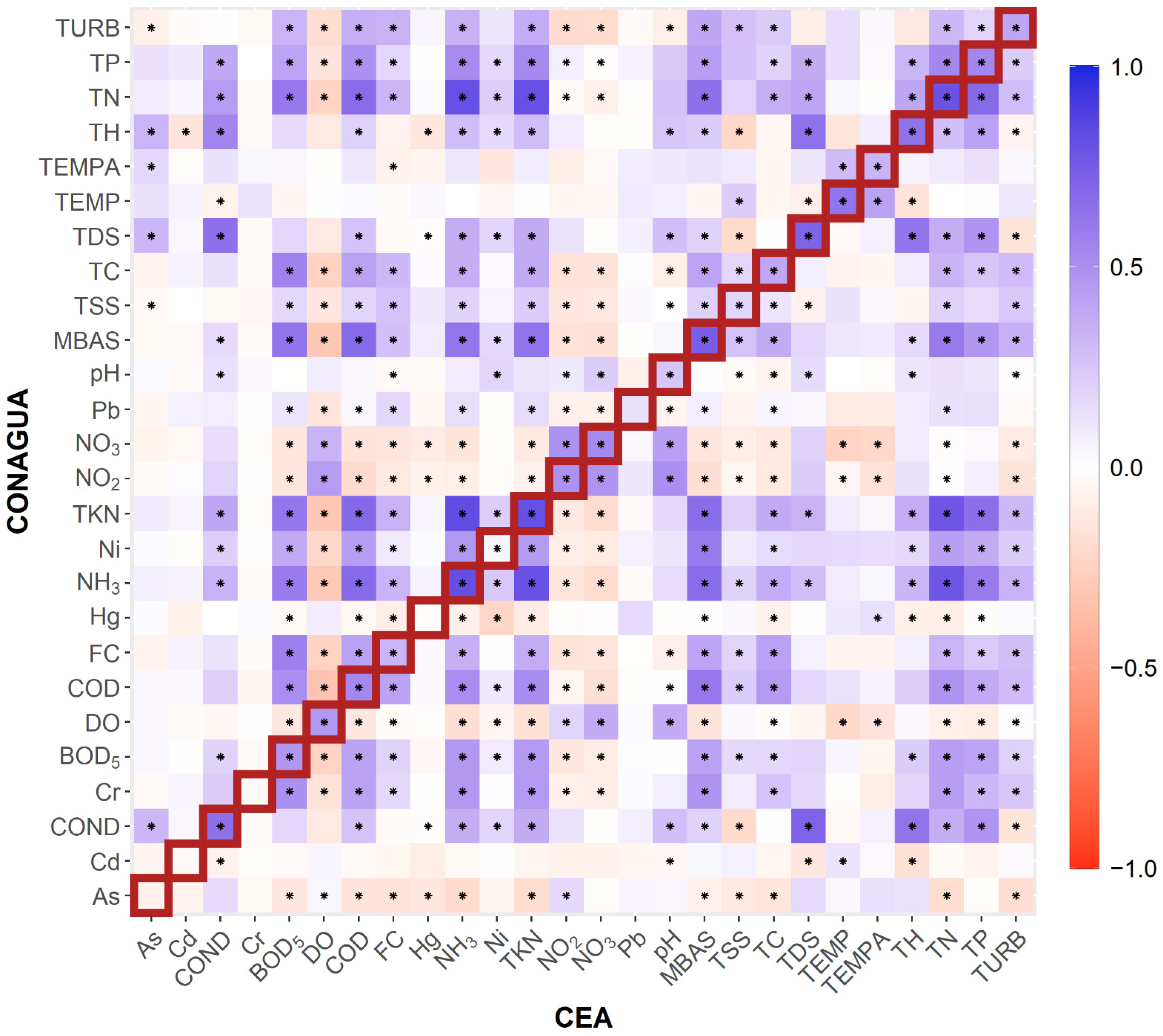
2.4.1. Principal Component and Correlation Analyses to Assess the Rationalization Potential of the Water Quality Parameters

Principal component analysis (PCA) was used for the identification of groups of highly correlated water quality parameters monitored by one or both authorities. PCA is a multivariate statistical technique used to reduce the dimensionality of water quality datasets and to maximize the variance by calculating novel uncorrelated variables, called the components, as linear functions of those in the original dataset [5,24]. This reduction occurs when there is substantial redundancy between the data, and therefore, a reduced number of elements can often explain most of the information [10]. To perform PCA, a multivariate random vector $X=\left(X_1,X_2,\dots ,X_n\right)$ with mean $\mathsf{\mu }$ and covariance $\mathsf{\Sigma }$ was considered. In this study, such a multivariate vector is given by the water quality parameters. Thus, $n$ different linear combinations of $X$ were obtained as:

$$Y_i={\displaystyle \sum }_{j=1}^n{\varphi }_{ij}{X}_j$$

(1)

For suitable multipliers ${\varphi }_{ij}$ resulting in $n$ components $Y_i$, $i=1,\dots , n$, of $X$. The weights ${\varphi }_{ij}$ are chosen so that the $y_i$ have the largest possible variances, are mutually orthogonal, and have a unit length so that ${\sum }_{j=1}^n{\varphi }_{ij}^2=1$. In this study, the PCA was used to identify the main parameters responsible for explaining the greater variability of water quality and the different sources of pollution. Biplots were constructed to ease the interpretation of the correlations among parameters, where each vector represents a monitored parameter within the dataset, and its length reflects the variance of the parameter. Vectors presenting smaller angle differences exhibit higher correlation than those with larger angle differences [25]. Four independent biplots were developed in this study: (i) the first one with the subset of water quality parameters measured exclusively by CONAGUA; (ii) the second one with the subset of water quality parameters measured by CEA; (iii) the third one with the subset of water quality parameter measured by both authorities, which showed consistency (high correlation) between authorities; and (iv) the fourth one with the subset of water quality parameter measured by both authorities but failed to show consistency (low correlation) between authorities.

Pearson correlation analyses were performed to test the correlations between the water quality parameters measured by both CEA and CONAGUA (Figure 3) with a focus on the comparison of neighboring monitoring sites (Table 1) to test the pairwise observations made by these authorities [26]. The temporal resolution of both data sets (CONAGUA and CEA) was considered, and only temporally and spatially paired observations were used to test the comparability of the time-corresponding data in neighboring monitoring sites. The Pearson’s correlation coefficient was calculated as follows:

$$r_{xy}=\frac{{\sum }_{i=1}^n\left(x_i-\overline{x}\right)\left(y_i-\overline{y}\right)}{\left(n-1\right){\mathsf{\sigma }}_x{\mathsf{\sigma }}_y}$$

(2)

where $\overline{x}$ and $\overline{y}$ denote the sample means, ${\mathsf{\sigma }}_x$ and ${\mathsf{\sigma }}_y$, are the sample standard deviations, and $\left(x_1,y_1\right),\left(x_2,y_2\right),\dots ,\left(x_n,y_n\right)$ are a set of $n$ observed pairs of pairwise observations of two water quality parameters at neighboring monitoring sites.

2.4.2. Cluster and Discriminant Analyses to Assess the Rationalization Potential of the Monitoring Sites

Cluster analysis (CA) was used to group the 15 (CONAGUA) and 20 (CEA) monitoring sites according to the spatial similarity of water quality. CA is frequently used to find monitoring sites that respond similarly to different sources of pollution affecting water quality, as it allows determination of clusters of monitoring sites, where the within-cluster variance is minimized, and the between-cluster variance is maximized. The resulting clusters display low heterogeneity, while objects from different clusters would show high external heterogeneity [26]. The clustering criteria was the silhouette index, $S_i\in \left[-1,1\right]$, which can estimate the goodness-of-fit and validate the number of clusters formed. The optimal number of clusters $k$ is the one that maximizes the average silhouette over a range of possible values for $k$ [27]. An average silhouette index greater than or equal to 0.27 as well as absence of negative values were the criteria considered to delineate the most appropriate number of groups [3]. To define the silhouette index $s\left(i\right)$ for the $i\mathrm{th}$ observation of water quality parameters, A was denoted as the cluster to which the $i\mathrm{th}$ has been assigned, and the average similarity $\mathrm{a}\left(i\right)$ of $i$ to all other objects of A was calculated. Then, the measure of dissimilarity was given by the Euclidean distance. Then, C was denoted as any other cluster different from A, and the average dissimilarity of $i$ to all objects of C, $d\left(i,C\right),$ was computed. After computing $d\left(i,C\right)$ for all clusters $C \ne A$, the smallest of all was selected$:$

$$b\left(i\right)=\underset{C\ne A}{\min } d\left(I,C\right)$$

(3)

Then, the silhouette index $s\left(i\right)$ was obtained as follows:

$$s\left(i\right)=\frac{b\left(i\right)-a\left(i\right)}{\max \left\{a\left(i\right),b\left(i\right)\right\}}$$

(4)

A dendrogram was constructed to ease the interpretation of the CA. The dendrogram allows for the identification of the monitoring sites that present high homogeneity in water quality (monitoring sites in the same cluster) and those with high heterogeneity (monitoring sites belonging to different clusters) [10].

Discriminant analysis (DA) was then used as a validation measure to test the discriminating ability of the clusters determined by CA. Linear discriminant analysis (LDA) was used to determine the probability of an observation or a set of observations belonging to each class (cluster) as follows:

$$f_k\left(X\right)\equiv \mathrm{Pr}\left(X|Y=k\right)$$

(5)

where $Y$ is the qualitative response variable (in this case the clusters), $X$ represents the set of water quality parameters, and $k$ represents the classes (cluster $A, B, \dots , K$). Linear discriminant analysis may be used to determine the probability of an observation belonging to the kth class given the predictors’ observations. Then, the Bayes’ theorem states:

$$\mathrm{Pr}\left(Y=k|X=x\right)=\frac{{\pi }_k{f}_k\left(x\right)}{{\sum }_{l=1}^k{\pi }_l{f}_l\left(x\right)}$$

(6)

where $f_k\left(x\right)$ is the density function, and ${\pi }_k$ is the prior probability of an observation of belonging to the $k\mathrm{th}$ class [28].

Discriminant analysis (DA) is somewhat like CA except that in DA, the groups (or clusters) are already known (as determined by CA), and the user is testing the ability of a set of variables to discriminate between the clusters [2]. Scatterplots were used to display the scores of the two first linear discriminant functions resulting from the DA to aid the visual interpretation of the clusters.

The multivariate statistics were performed using the programming language for statistical computing R (4.1.2) and the RStudio 1.4 IDE. The packages used were: tidyverse, ggdendro, corrplot, ggcorrplot, FactoMineR, factoextra, multcomp, clustertend, NbClust, pvclust, fpc, lubridate, openxlsx, and ggpubr. Geospatial analyses were performed in QGIS 3.20.2.

3. Results and Discussion

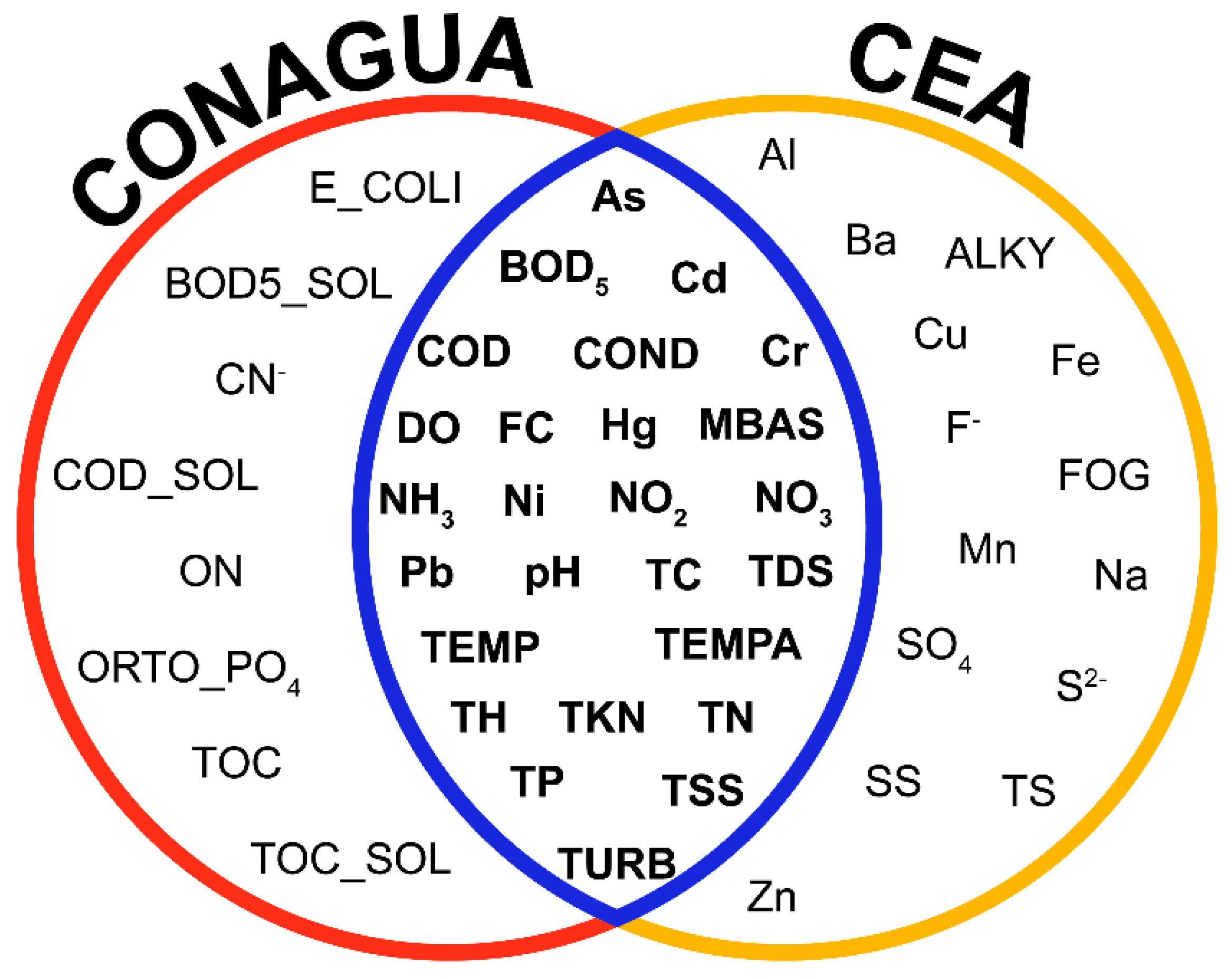
3.1. Rationalization of the Water Quality Parameters Currently Measured by Both Authorities

This section discusses the rationalization potential of the water quality parameters to identify those that could be discontinued from the monitoring program of at least one of the authorities without substantial information loss as well as potentially to start monitoring emerging water quality parameters not currently measured in the LSHS by either of the authorities. As depicted in Figure 3, there is a subset of water quality parameters that is currently measured by both authorities. Furthermore, these parameters are, in some cases, measured at neighboring monitoring sites with a proximity of 1 km or less (Table 1).

As seen in Figure 4, the pairwise observations of the water quality parameters made by both authorities at neighboring sites, shown in the diagonal, are highly correlated. Of the 26 coinciding parameters in the matrix diagonal, there were 21 pairs that presented significant correlations between the CEA and CONAGUA datasets. While these significant correlations evidence the consistency of the observations made by both authorities at neighboring sites; the same information is produced by both authorities. Additionally, typical correlations among different water quality parameters (outside of the diagonal) are present in Figure 4. Organic pollution-related parameters, such as BOD₅, TN, and TP, are highly correlated. In the same manner, DO displayed consistent negative correlations with pollutants known to decrease oxygen availability (such as BOD_5, COD, and TSS) and to contribute to eutrophication processes (such as TN and TP). If two water quality parameters are highly correlated, it means some of the information may be redundant, and perhaps one could stop measuring one of these two highly correlated variables (and potentially estimate its value from the remaining one). The parameters that should continue to be measured must be identified based on their significance, the stakeholders’ preference, or the presence of the parameters in local or international standards [29]. Discarding variables is not only convenient from a pragmatic standpoint (reducing costs, equipment, and time) but also to simplify the analysis through the elimination of information redundancies [30] and to include new parameters, such as emerging pollutants, such as antibiotics, surfactants, hormones, endocrine-disrupting compounds, and fire retardants, among others. These compounds have major impacts on terrestrial and aquatic ecosystems and human life owing to their acute and chronic toxicities and thus should be monitored in WQMNs [31].

The pairwise measurements of water quality parameters by both WQMNs may also limit the interpretation of the water quality data due to the generation of different or even contradicting observations between WQMNs. As seen in Figure 4, there were some inconsistencies among the data reported by these two independent WQMNs for five pairs of coinciding parameters (in the matrix diagonal), all of them heavy metals, which displayed nonsignificant correlations (As, Cd, Cr, Hg, and Pb). These nonsignificant correlations among coinciding parameters indicate possible inconsistencies in the data reported by CEA and CONAGUA for the parameters measured at neighboring monitoring sites. While these inconsistencies may result from the presence of point sources of pollution within the range of the monitoring sites, which may alter the representativeness of the actual conditions of the monitoring site [32], these differences frequently derive from differences in the analytical or sampling methods used by each authority, as each laboratory is equipped with its own instrumentation and personnel and therefore presents different calibration and sensitivity ranges [32].

As an example, Figure 5 presents the temporal trends of selected coinciding parameters measured by both authorities at one pair of neighboring sites (A03 and AA01). The temporal trend of Cr reported by both authorities is displayed in Figure 5a, which also displayed a nonsignificant correlation in Figure 4. The difference in the detection limits achieved by the different authorities can be clearly seen for the case of Cr. Furthermore, even when the observations made by CONAGUA were above the CEA limit of detection in 2016 and 2017, there were inconsistencies in the results reported by both authorities, as CONAGUA failed to report these higher concentrations of Cr.

In contrast, Figure 5b displays the temporal pairwise observations made by both authorities for COND. They are highly consistent and reflect the behavior over the year of this water quality parameter. This consistent behavior reported by both authorities is also depicted as a significant correlation for COND in Figure 4. The pairwise measurements made by both authorities for FC (Figure 5c) also displayed inconsistencies, as an increasing trend was reported by CEA from 2015 but not by CONAGUA. The report of pairwise measurements by CEA and CONAGUA that are different or contradicting shows a clear lack of communication between these authorities. The implementation of efficient communication networks among these authorities can greatly increase the effectiveness of the WQMNs. Information generated by the monitoring programs should be efficiently processed and uploaded into information systems to provide decision makers and stakeholders accurate and clear information [32].

To assess further the redundancies between the water quality parameters measured by both authorities, a PCA was developed to assess inter-parameter associations to identify parameters that might potentially serve as indicators of a wider set of parameters [30]. As shown by Figure 6, the water quality parameters measured exclusively by CEA (Figure 6a) and CONAGUA (Figure 6b) displayed the expected correlations between water quality parameters. The typically correlated physical parameters (TSS, TURB, COND, TH, and TDS) are highly correlated in both datasets. The correlation between nutrient-related parameters (NKJ, NH₃, TN, N_ORG, TP, and PO4) is another indicator of the proper distribution of the vectors of the water quality parameters among both datasets. Microbiological parameters (E. coli, FC, and TC) and heavy metals (Hg, Pb, Cr, Cd, Cu, Zn, and Ni) were also found to be highly correlated in both datasets. Furthermore, the oxygen-depletion parameters (DBO, DQO, DQO_SOL, and OD) were also highly correlated.

Regarding the water quality parameters that are measured independently by both authorities (CEA and CONAGUA), the vectors of the water quality observations made by both authorities displayed almost perfect correlations (Figure 6c), indicating that most water quality parameters measured both by CEA and CONAGUA are consistent. For instance, Figure 6c shows that the vector of measurements made for COND by CONAGUA (vector in red) and the vector of measurements made by CEA (vector in yellow) produce a very small angle, which reflects a perfect correlation. However, the vectors of heavy metals (Cr, Ni, Pb, Hg, and As), shown in Figure 6d, presented larger angles and exhibited lower correlation than those in Figure 6c.

3.2. Rationalization of the Monitoring Sites for a Possible Joint WQMN

The selection of appropriate monitoring sites is the most crucial task in designing WQMNs. Clustering analysis allowed for the assessment of similarities (and dissimilarities) among monitoring sites regarding their water quality features [26,32]. Figure 7 presents the resulting dendrogram for the combined set of monitoring sites from both WQMNs considering only the water quality parameters measured by both authorities (those in the blue region of Figure 3). Independent clusters reflect different water quality conditions throughout the LSHS. The monitoring sites in the same group are considered to reflect similar water features. Moreover, when neighboring monitoring sites are allocated in the same cluster these can be considered to produce redundant information in relation to the water quality parameters.

The monitoring sites located within the same sub-basins were grouped together because they share similar water quality features, as can be generally seen in Figure 7, largely due to their land cover distribution (Figure 2), which has a direct effect in water quality (Fiquepron et al., 2013). The monitoring sites located in highly urban and industrial sub-basins, such as RH2Eb (with clusters H, I, J, and K), or in highly forested sub-basins, such as RH12Ed andRH12Ej (with cluster E), were clustered together, respectively, as seen in Figure 7. Forested areas are known to have a positive effect on surface water resources by the retention of pollutants and the reduction of runoff rates [33,34]. Conversely, industrial and urban areas are prone to surface pollutant transport due to low surface permeability and increased surface runoff [35,36] as well through storm water discharge pipes or industrial discharge (legal or illegal)

Monitoring sites RZ-05-CEA, RZ-04-CEA, and AA-01-CEA, which correspond to cluster A, B, and G, respectively, were found to produce unique water quality features, which are different from most other monitoring sites. Furthermore, it is interesting to note that the clusters A and G (corresponding to the RZ-05-CEA and AA-01-CEA monitoring sites, respectively) are those with the greatest Euclidean distance in relation to the other clusters, indicating a large difference in water quality between them. Clusters A and B are located within the RH12Ee, which presents one of the largest areas of agricultural land cover (84%) and is known to have one of the highest livestock densities in the state. Cluster G is located downstream of the MAG and the El Ahogado wastewater treatment plant, which receives most of the urban wastewater and runoff produced in the MAG. Agricultural and municipal pollution are significant contributors to pollution of the Santiago River that explain the cluster patterns shown in Figure 7 [33,36,37].

Figure 7 shows that most pairs of neighboring sites were grouped within the same cluster. This not only indicates that most of the neighboring monitoring sites share similar water quality features but also highlights the duplicated efforts of these overlapping WQMNs [26]. The pairs of neighboring sites that were not clustered together can be related to the analytical methods employed to evaluate specific water quality parameters by both authorities (CEA and CONAGUA), specifically heavy metals. For instance, both AA1-A03 and RL02-L07 neighboring pairs are in industrialized urban areas, that are highly polluted by heavy metals. However, the methods used by each authority for the determination of these pollutants as well as their detection limits can significantly differ, as presented in Figure 5a for the case of Cr. The method employed by CEA for heavy metal detection is atomic absorption spectrometry (AAS); however, this method has the limitation of relatively high detection limits (in the range of µg/L) [38]. CONAGUA uses inductively coupled plasma—atomic emission spectrometry (ICP-AES) and inductively coupled plasma—mass spectrometry (ICP-MS), which has detection limits in the range of ng/L or lower [39]. These unclustered neighboring sites are in heavily urbanized and industrial sub-basins, as displayed by Figure 2 (RH12Eb and RH12Cb for AA1-A03 and RL02-L07, respectively), in which previous studies have reported heavy metal pollution.

While the cluster analysis indicates the monitoring sites eligible for exclusion following a statistical approach, the optimization of the WQMNs does not necessarily imply reduction in the number of monitoring sites, as these sites may serve other purposes, such as trend analysis, establishment of reference conditions, and water body representativeness. Some monitoring sites may be located downstream of major pollution sources to account for the effect of anthropogenic activities (mostly in terms of point sources of pollution [30]. Therefore, a careful territorial analysis must be made before deciding on the exclusion of specific monitoring sites.

The LDA was used as a validation procedure for the cluster analysis (Figure 8). Figure 8c displays the scatterplot for the scores resulting for the spatial DA and suggests that the linear discriminant functions correctly assign the water quality observations to the clusters; thus, the water quality observations offer enough information to discriminate between the previously identified clusters. Figure 8a,b are displayed as proof of the overall inconsistencies regarding the measurement of heavy metals by both authorities. Figure 8a was developed to test the ability of the discriminant functions to classify water quality observations between the authorities when heavy metals were considered, while Figure 8b was developed to test the ability of the discriminant functions to classify water quality observations between authorities when heavy metals were not considered. As shown in these figures, there is overall consistency between authorities for most water quality parameters except for heavy metals.

3.3. Main Deficiencies of the WQMNs within the Context of the LSHS and Potentialities for Developing Countries

Any new configuration of the WQMNs must be based on a cost-effective and targeted approach. The resource optimization from the readjustment of the WQMNs can be an opportunity for the expansion of the network either spatially, by the addition of new relevant monitoring stations, or analytically, by the expansion of water quality parameters within the network. Since all the current monitoring sites are located on the main stream of LSHS, the system information can be enriched with monitoring sites located on the tributaries. A geostatistical approach can be useful to propose new locations based on geographic, hydrological, pollution source, and population data [40]. The water quality data monitored at these new locations can be analyzed using multivariate analysis to discard sites with redundant information and maintain monitoring at sites providing the most valuable information through an iterative approach. Currently, CEA and CONAGUA only monitor traditional physical, chemical, and biological parameters (Figure 3); however, with rising interest in emerging pollutants [31,32], developing countries have the possibility to redesign and optimize current WQMNs and expand their monitoring capabilities to new high-interest parameters without significantly increasing operational costs [32]. The incorporation of emerging contaminants in the LSHS WQMN must be based on the level of concern. The most concerning contaminants may be incorporated in the permanent WQMN, while those of less concern may be monitored with a lower frequency. Highly concerning contaminants include pesticides, plasticizers, polyaromatic hydrocarbons (PAH), flame retardants, pharmaceuticals, antibiotics, personal care products, microplastics, and other persistent organic pollutants (POPs). Scrutiny and future regulation should be based on persistence level and the effect severity of the effects on ecosystems and human health [41,42].

Because the databases were not homogeneous (i.e., not all parameters are sampled at all monitoring sites and the sampling frequency differs), there is a need to adopt a unified sampling frequency in both WQMNs. However, due to the high costs of a monthly sampling frequency as adopted by CEA, a monthly frequency may only be adopted by CONAGUA for priority parameters at the monitoring sites. The harmonization among sampling frequencies between WQMNs allows for the comparison between stations and between different territories as well as for the determination of optimal sampling frequencies based on previously obtained data [32].

The sampling and laboratory methodologies used for the determination of many of the variables integrating the WQMNs are highly sensitive to non-homogeneities derived from environmental and anthropogenic variables related to the organization and operation of each WQMN. For instance, as discussed in Section 3.1, there are inconsistencies in the values reported by both authorities for heavy metals due to differences in the detection limits in each authority.

To increase the quality of the collected data, these interacting WQMNs should coordinate efforts and resources to harmonize methodologies (sampling frequencies and analytical methods, equipment, detection limits, etc.) [26,32]. The recommendation for heavy metal determination in the LSHS is the standardization of a common technique between both authorities involved in water quality monitoring. Moreover, harmonizing the monitoring objectives opens up a debate about which authority should monitor which parameters. This could be a political and bureaucratic obstacle to the rationalization of the monitoring program, whereas harmonizing monitoring sites, sampling frequency, and water quality parameters could be a more fruitful endeavor.

All harmonization efforts may be useless if a clear channel of communication and collaboration among the participating authorities is lacking. The establishment of transparent and accessible information platforms would allow for a better exploitation of the collected data and for clear and efficient use of the obtained information by policymakers and relevant stakeholders [26,32]. This approach requires the cooperation between the local and national authorities involved in the LSHS management. The creation of communication channels (e.g., online databases, webpage fora or panels, decision support systems) for the systematic exchange of information, experience, and good practices is highly recommended. An optimal channel should facilitate communication between researchers and decision makers [43]. However, applicability of this approach is challenging in developing countries, where economic, institutional, political, and social conditions are unstable. This situation can lead to failures in monitoring programs, as the optimal implementation requires a strong and long-term cooperation and coordination between all the stakeholders involved.

WQMN in developing countries are often limited by financial resources and technical capabilities and therefore have to prioritize resource allocation [1]. Optimization of monitoring sites, water quality parameters, and sampling frequency are common strategies for cost reduction from WQMNs [32]. Similar to the results herein presented, other studies have reported efforts in WQMN optimization. For instance, Noori et al. [44] and Noori et al. [45] conducted studies where monitoring sites were removed from a WQMN in Iran due to redundancies observed in the data matrix, and specific water quality parameters were selected as relevant based on their temporal variation. Resource reallocation presents greater opportunities for developing countries with multiple WQMNs, where harmonization strategies can lead to significant cost reductions, extended network reach, and higher overall data quality [32].

4. Conclusions

The present case study highlights the duplication in effort to monitor surface water quality in the LSHS basin, showing a lack of coordination between the authorities. The rationalization potential showed that water quality parameters could be discontinued from the monitoring program of at least one of the authorities without substantial information loss and potentially to start monitoring emerging water quality parameters not currently measured in the LSHS by either of the authorities. The multivariate analysis indicated those monitoring sites eligible for exclusion that would allow for the expansion of other parts of the LSHS not currently monitored, including relevant tributaries to the LSHS, which are not currently monitored.

However, the redesign and potential expansion of the joint WQMN should consider local conditions, such as available financial resources, land use, and legal requirements. Furthermore, using the case study of the LSHS in Mexico, we examined various deficiencies such as the use of different sampling frequencies and analytical methods by the authorities and lack of communication systems among stakeholders within the context and feasibilities in developing countries and proposed possible solutions to improve the performance of the joint WQMN.

References

1. Trevathan, J.; Atkinson, I.; Read, W.; Johnstone, R.; Bajema, N.; McGeachin, J. Establishing Low Cost Aquatic Monitoring Networks for Developing Countries. In Communications: Wireless in Developing Countries and Networks of the Future; Pont, A., Pujolle, G., Raghavan, S.V., Eds.; Springer: Berlin/Heidelberg, Germany, 2010; pp. 39–50. [Google Scholar] [CrossRef] [Green Version]
2. Khalil, B.; Ouarda, T.B.M.J. Statistical approaches used to assess and redesign surface water-quality-monitoring networks. J. Environ. Monit. 2009, 11, 1915–1929. [Google Scholar] [CrossRef] [PubMed]
3. De Almeida, R.G.B.; Lamparelli, M.C.; Dodds, W.K.; Cunha, D.G.F. Spatial optimization of the water quality monitoring network in São Paulo State (Brazil) to improve sampling efficiency and reduce bias in a developing sub-tropical region. Environ. Sci. Pollut. Res. 2022, 29, 11374–11392. [Google Scholar] [CrossRef] [PubMed]
4. Calazans, G.M.; Pinto, C.C.; da Costa, E.P.; Perini, A.F.; Oliveira, S.C. The use of multivariate statistical methods for optimization of the surface water quality network monitoring in the Paraopeba river basin, Brazil. Environ. Monit. Assess. 2018, 190, 491. [Google Scholar] [CrossRef]
5. Casillas-García, L.F.; de Anda, J.; Yebra-Montes, C.; Shear, H.; Díaz-Vázquez, D.; Gradilla-Hernández, M.S. Development of a specific water quality index for the protection of aquatic life of a highly polluted urban river. Ecol. Indic. 2021, 129, 107899. [Google Scholar] [CrossRef]
6. CONAGUA. Calidad del agua en México 2021. Available online: http://www.gob.mx/conagua/articulos/calidad-del-agua (accessed on 2 February 2022).
7. CEA. Sistema de Calidad Del Agua-CEA Jalisco 2022. Available online: http://info.ceajalisco.gob.mx/sca/ (accessed on 1 February 2022).
8. Rizo-Decelis, L.D.; Andreo, B. Water Quality Assessment of the Santiago River and Attenuation Capacity of Pollutants Downstream Guadalajara City, Mexico. River Res. Appl. 2016, 32, 1505–1516. [Google Scholar] [CrossRef]
9. Rizo-Decelis, L.D.; Pardo-Igúzquiza, E.; Andreo, B. Spatial Prediction of Water Quality Variables along a Main River Channel, in Presence of Pollution Hotspots. Sci. Total Environ. 2017, 605–606, 276–290. [Google Scholar] [CrossRef]
10. Calazans, G.M.; Pinto, C.C.; da Costa, E.P.; Perini, A.F.; Oliveira, S.C. Using Multivariate Techniques as a Strategy to Guide Optimization Projects for the Surface Water Quality Network Monitoring in the Velhas River Basin, Brazil. Environ. Monit. Assess. 2018, 190, 726. [Google Scholar] [CrossRef]
11. Mavukkandy, M.O.; Karmakar, S.; Harikumar, P.S. Assessment and Rationalization of Water Quality Monitoring Network: A Multivariate Statistical Approach to the Kabbini River (India). Environ. Sci. Pollut. Res. 2014, 21, 10045–10066. [Google Scholar] [CrossRef]
12. Peña-Guzmán, C.A.; Soto, L.; Diaz, A. A Proposal for Redesigning the Water Quality Network of the Tunjuelo River in Bogotá, Colombia through a Spatio-Temporal Analysis. Resources 2019, 8, 64. [Google Scholar] [CrossRef] [Green Version]
13. Mahjouri, N.; Kerachian, R. Revising River Water Quality Monitoring Networks Using Discrete Entropy Theory: The Jajrood River Experience. Environ. Monit. Assess. 2011, 175, 291–302. [Google Scholar] [CrossRef]
14. Aparicio, J. Hydrology of the Lerma-Chapala Watershed. In The Lerma-Chapala Watershed; Springer: Boston, MA, USA, 2001; pp. 3–30. [Google Scholar] [CrossRef]
15. CONAGUA. Programa de medidas preventivas y de mitigación de la sequía en la cuenca Lerma-Chapala. 2015. Available online: https://www.gob.mx/conagua/acciones-y-programas/programas-de-medidas-preventivas-y-de-mitigacion-a-la-sequia-pmpms-por-consejo-de-cuenca (accessed on 1 February 2022).
16. McCulligh, C.; Arellano-García, L.; Casas-Beltrán, D. Unsafe waters: The hydrosocial cycle of drinking water in Western Mexico. Local Environ. 2020, 25, 576–596. [Google Scholar] [CrossRef]
17. CONABIO. Mapa Nacional de Referencia, Cobertura de Suelo, 1:20000. INEGI, CONAFOR. 2018. Available online: https://monitoreo.conabio.gob.mx/snmb_charts/descarga_datos_madmex.html (accessed on 1 February 2022).
18. Gebhardt, S.; Maeda, P.; Wehrmann, T.; Argumedo Espinoza, J.; Schmidt, M. A proper Land Cover and Forest Type Classification Scheme for Mexico. In The International Archives of the Photogrammetry, Remote Sensing and Spatial Information Sciences; Copernicus GmbH: Göttingen, Germany, 2015; pp. 383–390. [Google Scholar] [CrossRef] [Green Version]
19. Sutadian, A.D.; Muttil, N.; Yilmaz, A.G.; Perera, B.J.C. Development of a water quality index for rivers in West Java Province, Indonesia. Ecol. Indic. 2018, 85, 966–982. [Google Scholar] [CrossRef]
20. American Public Health Association; American Water Works Association; Water Pollution Control Federation (Eds.) Standard Methods: For the Examination of Water and Wastewater, 20th ed.; American Public Health Association: Washington, DC, USA, 1998. [Google Scholar]
21. American Public Health Association; American Water Works Association; Water Environment Federation (Eds.) Standard Methods for the Examination of Water and Wastewater, 21st ed.; American Public Health Association: Washington, DC, USA, 2005. [Google Scholar]
22. EMA. ¿Qué Es Ema? 2022. Available online: https://www.ema.org.mx/portal_v3/index.php/que-es-ema (accessed on 2 February 2022).
23. Little, R.J.A.; Rubin, D.B. Statistical Analysis with Missing Data, 3rd ed.; Wiley: Hoboken, NJ, USA, 2020. [Google Scholar]
24. Gradilla-Hernández, M.S.; de Anda, J.; Garcia-Gonzalez, A.; Meza-Rodríguez, D.; Yebra Montes, C.; Perfecto-Avalos, Y. Multivariate water quality analysis of Lake Cajititlán, Mexico. Environ. Monit. Assess. 2019, 19, 5. [Google Scholar] [CrossRef]
25. Zuur, A.F.; Ieno, E.N.; Smith, G.M. Analysing Ecological Data; Statistics for Biology and Health; Springer: New York, NY, USA, 2007; ISBN 978-0-387-45972-1. [Google Scholar]
26. Chapman, D.V.; Bradley, C.; Gettel, G.M.; Hatvani, I.G.; Hein, T.; Kovács, J.; Liska, I.; Oliver, D.M.; Tanos, P.; Trásy, B.; et al. Developments in water quality monitoring and management in large river catchments using the Danube River as an example. Environ. Sci. Policy 2016, 64, 141–154. [Google Scholar] [CrossRef] [Green Version]
27. Kaufman, L.; Rousseeuw, P.J. Finding Groups in Data: An Introduction to Cluster Analysis; John Wiley & Sons: Hoboken, NJ, USA, 2009. [Google Scholar]
28. James, G.; Witten, D.; Hastie, T.; Tibshirani, R. An Introduction to Statistical Learning: With Applications in R, 2nd ed.; Springer: New York, USA, 2021. [Google Scholar]
29. Khalil, B.; Ouarda, T.B.M.J.; St-Hilaire, A.; Chebana, F. A Statistical Approach for the Rationalization of Water Quality Indicators in Surface Water Quality Monitoring Networks. J. Hydrol. 2010, 386, 173–185. [Google Scholar] [CrossRef]
30. Varekar, V.; Yadav, V.; Karmakar, S. Rationalization of water quality monitoring locations under spatiotemporal heterogeneity of diffuse pollution using seasonal export coefficient. J. Environ. Manag. 2021, 277, 111342. [Google Scholar] [CrossRef]
31. Vasilachi, I.C.; Asiminicesei, D.M.; Fertu, D.I.; Gavrilescu, M. Occurrence and Fate of Emerging Pollutants in Water Environment and Options for Their Removal. Water 2021, 13, 181. [Google Scholar] [CrossRef]
32. Harmancioglu, N.B.; Ozkul, S.D.; Alpaslan, M.N. Water Quality Monitoring and Network Design; Springer: Dordrecht, The Netherlands, 1998; pp. 61–106. [Google Scholar] [CrossRef]
33. Fiquepron, J.; Garcia, S.; Stenger, A. Land use impact on water quality: Valuing forest services in terms of the water supply sector. J. Environ. Manag. 2013, 126, 113–121. [Google Scholar] [CrossRef]
34. Kreye, M.M.; Adams, D.C.; Escobedo, F.J. The Value of Forest Conservation for Water Quality Protection. Forests 2014, 5, 862–884. [Google Scholar] [CrossRef] [Green Version]
35. Hall, M.J.; Ellis, J.B. Water Quality Problems of Urban Areas. GeoJournal 1985, 11, 265–275. [Google Scholar] [CrossRef]
36. McGrane, S.J. Impacts of Urbanisation on Hydrological and Water Quality Dynamics, and Urban Water Management: A Review. Hydrol. Sci. J. 2016, 61, 2295–2311. [Google Scholar] [CrossRef]
37. Diaz-Vázquez, D.; Cummings, S.C.A.; Rodríguez, D.M.; Guerrero, C.S.; de Anda, J.; Gradilla-Hernández, M.S. Evaluation of Biogas Potential from Livestock Manures and Multicriteria Site Selection for Centralized Anaerobic Digester Systems: The Case of Jalisco, México. Sustainability 2020, 12, 3527. [Google Scholar] [CrossRef]
38. Draghici, C.; Jelescu, C.; Dima, C.; Coman, G.; Chirila, E. Heavy Metals Determination in Environmental and Biological Samples. In Environmental Heavy Metal Pollution and Effects on Child Mental Development; Simeonov, L.I., Kochubovski, M.V., Simeonova, B.G., Eds.; Springer: Dordrecht, The Netherlands, 2011; pp. 145–158. [Google Scholar]
39. Moor, C.; Lymberopoulou, T.; Dietrich, V.J. Determination of Heavy Metals in Soils, Sediments and Geological Materials by ICP-AES and ICP-MS. Mikrochim. Acta 2001, 136, 123–128. [Google Scholar] [CrossRef] [Green Version]
40. Jiang, J.; Tang, S.; Han, D.; Fu, G.; Solomatine, D.; Zheng, Y. A Comprehensive Review on the Design and Optimization of Surface Water Quality Monitoring Networks. Environ. Model. Softw. 2020, 132, 104792. [Google Scholar] [CrossRef]
41. EC. European Parlament. Directive 2000/60/EC of the European Parliament and of the Council of 23 October 2000 Establishing a Framework for Community Action in the Field of Water Policy; Office for Official Publications of the European Communities: Luxembourg, 2000. Available online: https://www.eea.europa.eu/policy-documents/directive-2000-60-ec-of (accessed on 2 February 2022).
42. Dulio, V.; van Bavel, B.; Brorström-Lundén, E.; Harmsen, J.; Hollender, J.; Schlabach, M.; Slobodnik, J.; Thomas, K.; Koschorreck, J. Emerging Pollutants in the EU: 10 Years of NORMAN in Support of Environmental Policies and Regulations. Environ. Sci. Eur. 2018, 30, 5. [Google Scholar] [CrossRef]
43. Faby, J.-A.; Neveu, G.; Jacquin, N. Towards a European-Wide Exchange Network for Improving Dissemination of Integrated Water Resources Management Research Outcomes. Environ. Sci. Policy 2005, 8, 307–319. [Google Scholar] [CrossRef]
44. Noori, R.; Sabahi, M.S.; Karbassi, A.R.; Baghvand, A.; Taati Zadeh, H. Multivariate Statistical Analysis of Surface Water Quality Based on Correlations and Variations in the Data Set. Desalination 2010, 260, 129–136. [Google Scholar] [CrossRef]
45. Noori, R.; Karbassi, A.; Khakpour, A.; Shahbazbegian, M.; Badam, H.M.K.; Vesali-Naseh, M. Chemometric Analysis of Surface Water Quality Data: Case Study of the Gorganrud River Basin, Iran. Environ. Model. Assess. 2012, 17, 411–420. [Google Scholar] [CrossRef]
Figure 1. Distribution of the monitoring sites of the CEA and CONAGUA WQMNs within the LSHS.
Water 14 01687 g001
Figure 2. Distribution of the land-cover types within the subbasins of the LSHS based on CONABIO (2018) data.
Water 14 01687 g002
Figure 3. Ven diagram displaying the subsets of the water quality parameters measured by CONAGUA and CEA.
Water 14 01687 g003
Figure 4. Correlation matrix for the water parameters measured by both CONAGUA and CEA at neighboring monitoring sites.
Water 14 01687 g004
Figure 5. Time series plots of selected parameters, (a) Cr (b) COND, and (c) FC, with pairwise measurements by CONAGUA and CEA at neighboring monitoring sites (A03 and AA01).
Water 14 01687 g005
Figure 6. Biplots for the water quality parameters monitored by (a) CEA and (b) CONAGUA exclusively and (c,d) the parameters measured by both CEA and CONAGUA. The angles between two vectors reflect their correlations; the smaller the angle the greater the correlation.
Water 14 01687 g006
Figure 7. Dendrogram and spatial distribution map presenting the clusters of monitoring sites managed by CONAGUA and CEA. The clusters within the grey rectangles in the dendrogram group those monitoring sites with similar water quality features.
Water 14 01687 g007
Figure 8. Scatterplot for the scores of the two first linear discriminant functions using the standard method: (a) classification between authorities including heavy metals, (b) classification between authorities not including heavy metals, and (c) classification between clusters.
Water 14 01687 g008