A Comparative Analysis of Infiltration Models for Groundwater Recharge from Ephemeral Stream Beds: A Case Study in Al Madinah Al Munawarah Province, Saudi Arabia

Abstract

Groundwater recharge is strongly influenced by the infiltration process. In this research, the Philip, Horton, Kostiakov, and Green–Ampt infiltration models were tested for the ability to describe the infiltration process in the ephemeral stream beds located in Al Madinah Al Munawarah Province in Saudi Arabia. Infiltration data were obtained from double-ring infiltrometer tests in 14 locations distributed over the province. The method of least squares through an objective function optimization formalism is utilized to estimate the parameters of each model. The results show high variability in the parameters of each model over the tests. Individual tests showed that some models were better for representing specific tests than other models. On average, the Kostiakov empirical model was the best at describing the 14 infiltration tests with only 2 empirical parameters, since it had the minimum root mean square error (RMSE) for the cumulative infiltration depth F (1.13 cm), and it also had the same RMSE for the infiltration rates f (0.1 cm/min), similar to other models. Moreover, the Kostiakov model had an acceptable correlation coefficient R = 0.61 for f, and R = 0.99 for F. The results imply significant variability in the groundwater recharge rates from flash floods in the region.

1. Introduction

The infiltration process is defined as the vertical water movement from the ground surface into the soil [1]. This process takes place in the hydrological cycle when water moves on the ground as overland flows. Estimation of infiltration rates is of the utmost importance for runoff predictions, groundwater recharge estimation, and the designing of hydraulic and irrigation structures. In arid regions, the process of infiltration occurs frequently during the propagation of flash floods passing in the ephemeral streams on a dry bed [2].

Infiltration modeling is often categorized into two approaches, namely physically based and empirically based models. The physically based approaches require the solution of the Richards’ equation [3], which describes theoretically the movement of water into the soil. Richards’ equation can be expressed in different forms, and one of the commonly used expressions reads as follows:

$$\frac{\partial \theta }{\partial t}=\frac{\partial \theta }{\partial z}\left[D\left(\theta \right)\frac{\partial \theta }{\partial z}\right]-\frac{\partial K\left(\theta \right)}{\partial z}$$

(1)

where $\theta$ is the volumetric water content, $K\left(\theta \right)$ is the hydraulic conductivity as a function of the volumetric water content, $D\left(\theta \right)$ is called the soil diffusivity as a function of volumetric water content, and z is the depth below the soil surface.

Solving Equation (1) at specified initial and boundary conditions is rather difficult under some flow conditions and requires detailed input data. The solution uses numerical methods for solving nonlinear differential equations [4]. However, recently, the decomposition method could be used in the future to solve such nonlinear equations [5,6,7,8]. The Philip [9] and Green and Ampt [10] models are simpler models that emerged from Richards’ equation.

Among the empirically based models, there are the Horton [11,12] and Kostiakov models [13]. The Philip, Green and Ampt, Horton, and Kostiakov models are the most commonly used equations in hydrological research, engineering, and irrigation applications because of their simplicity and capability of fitting field infiltration data.

The published literature on infiltration studies through ephemeral streams in general, and in the Kingdom of Saudi Arabia (KSA) in particular, is limited. Some of the published literature is reviewed below.

Some studies estimated infiltration from rainfall-runoff data using some loss function techniques. The authors of [14] used the Φ-index method to estimate the infiltration losses from rainfall in the Yiba basin and found out that 93% of the rainfall was lost during the infiltration process at the catchment scale.

Some other studies focused on the estimation of infiltration from the transmission losses in ephemeral streams due to flood movement on the dry bed channel. The authors of [15] used the extended two-parameter Muskingum model to develop the three-parameter Muskingum model that incorporates transmission losses. They found out the maximum transmission could reach 84% of the incoming inflow to the channel’s reach in the Yiba basin located in the southwestern part of SA. The authors of [15] generalized the analytical solution given by Hayami [16] for modeling diffusive flood wave propagation in rivers to model flood waves in ephemeral streams, with transmission losses described by a decay parameter which was estimated to range between 0.43 and 1.4 h⁻¹ for the Yiba basin. This decay parameter describes the loss rate of the flood wave while passing through the ephemeral stream which is contributing to the infiltration process.

The authors of [17] performed hydrological modeling in Wadi Itwad in southwestern SA for flood hazard assessment. In the analysis, they carried out infiltration tests in the wadi alluvium to estimate the hydrological parameters of the ephemeral channel bed for curve number estimation and, consequently, estimation of the flood hazards. They used the Horton and Philp models to model the infiltration tests. The results show that the saturated hydraulic conductivity varied between 0.66 and 39.4 m/day for the Philip model, while it varied between 0.12 and 2.4 m/day based on the Horton model. It is quite clear that there was high variability either within a single model or even between the two models.

Recently, several researchers used new techniques such as neural networks and fuzzy logic to estimate the infiltration parameters for assessing the infiltration process and soil hydraulic properties, among those [18,19,20,21,22,23,24,25,26,27] who studied the influence of agriculture activities on infiltration. They concluded that agricultural activity can increase the hydraulic conductivity of the soil and, in turn, the water storativity due to the rainfall effect. In arid, sandy regions, deeper soil recharge replenishment occurs more during the rainy season than during the freeze-thaw seasons in winter and spring [28].

The main objectives of this paper are as follows:

-

To estimate the soil hydrological parameters (such as hydraulic conductivity, soil sorptivity, and initial infiltration rates) of the ephemeral stream bed that are useful for flood prediction, groundwater recharge, and irrigation studies in the Al Madinah Al Munawarah Province;

-

To perform a simple statistical analysis to estimate the spatial variability of the soil parameters from the field tests and obtain an overview regarding the degree of this variability. This is important in sensitivity and uncertainty analyses in rainfall-runoff modeling;

-

To test the best infiltration model (Philip, Horton, Kostiakov, and Green and Ampt) suited to interpreting the infiltration process in the ephemeral stream bed, utilizing field data from double-ring infiltrometer tests;

-

To recommend the best one to use in hydrological modeling in the arid region of Saudi Arabia and similar regions.

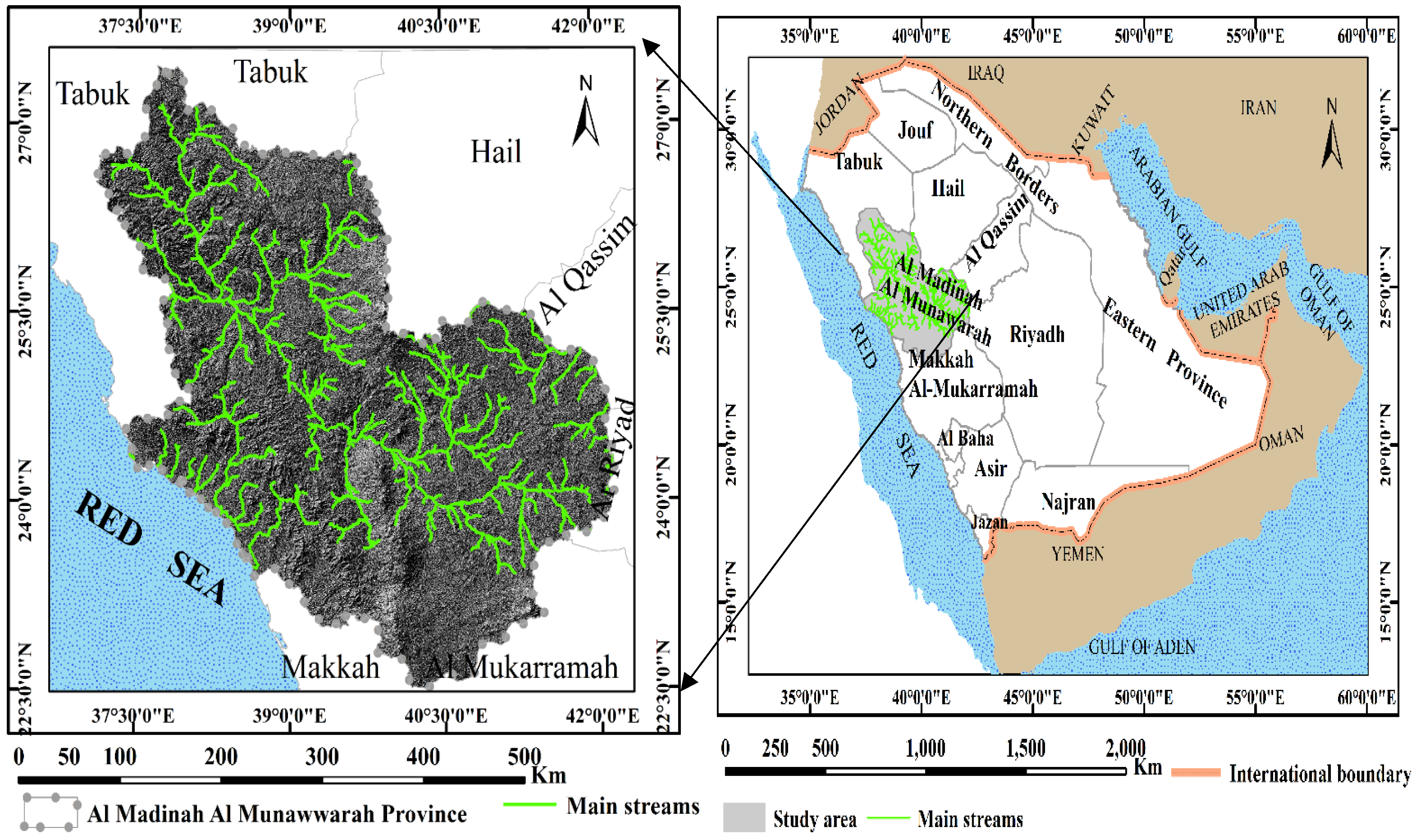
2. Study Area and Data Collection

Al Madinah Al Munawarah Province is located in the northern central part of Saudi Arabia. It is bounded by the provinces of Makkah Al-Mukarramah and Riyadh to the south, by the Red Sea in the west, by Tabuk Province in the north, and the provinces of Hail and Al Qassim to the east. The study province is restricted between latitudes 22°29′00″ and 27°29′00″ N and longitudes 37°27′00″ and 42°07′00″ E with an area of about 176,715.6 Km² and a perimeter of about 2900.2 km, as shown in Figure 1.

2.1. Climate

Climate is considered one of the main factors which influences the water resources and hydrological behavior of the hydrographic basins. According to [29], Saudi Arabia is characterized by distinguished climatic regions due to high spatial and temporal temperature variability. The study province of Al Madinah Al Munawarah, which extends from the Tihama-Asir coastal area of Saudi Arabia inland toward the northeast, has different climate and water conditions where, according to [30], the study area lies within an arid and hyper-arid sector of the desert, and it is influenced greatly by a highly mountainous area [31]. This study depended on 6 rainfall stations and 3 meteorological stations for a time duration ranging from 33 to 49 years. The parameters of air temperature, relative humidity, and evaporation were based on 3 meteorological stations over a duration of about 40 years (1973–2012), as shown in Figure 2.

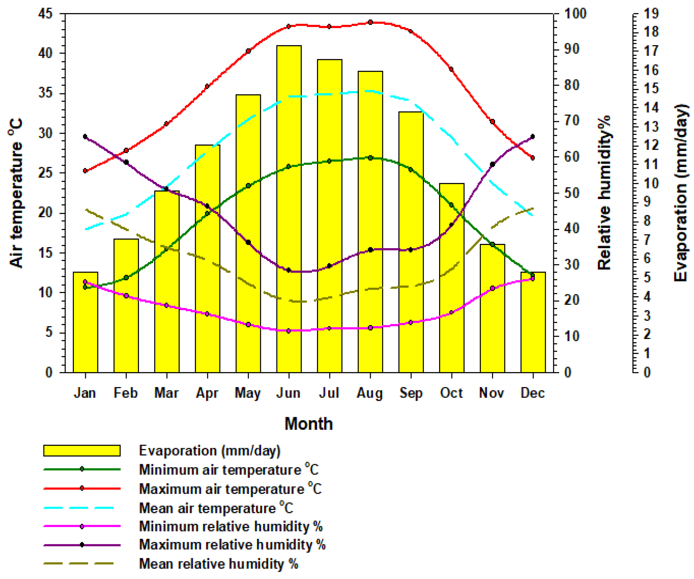
2.1.1. Air Temperature

Temperatures in the study area can vary both temporally and spatially, with hot summers and warm winters having mean air temperatures of 35.4 °C in August and 17.9 °C in January, as shown in Figure 2. According to [32], the spatial variations in air temperature are due to elevation variations, where the mountainous areas are characterized by low temperature values while the coastal areas are characterized by high temperatures.

2.1.2. Evaporation

Evaporation is an important meteorological parameter for determination of the initial water losses, especially from surface water. Evaporation is controlled by many other meteorological elements, such as air temperature, relative humidity, solar radiation, and wind speeds. Generally, the evaporation rate is high in the Kingdom of Saudi Arabia due to the arid conditions, and in the study province, it ranges from 5.33 mm/day in December and January to 17.3 mm/day in June, as shown in Figure 2.

2.1.3. Relative Humidity

The relative humidity is closely related to temperature, where it increases with a decrease in air temperature and decreases with an increase in air temperature. In the study province, the average relative humidity ranges from 19.9% in June to 45.8% in December, as shown in Figure 2.

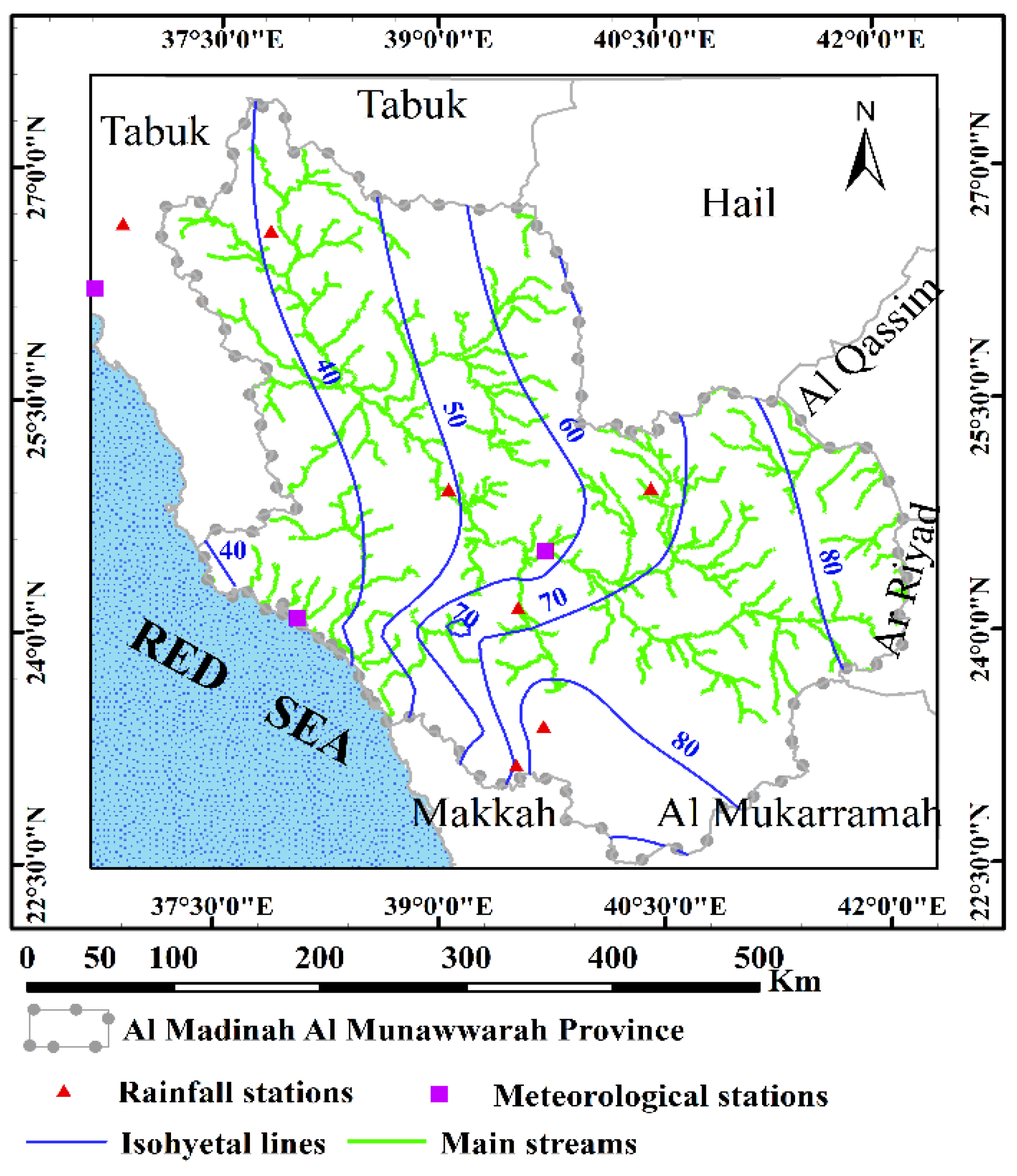
2.1.4. Rainfall

The study province of Al Madinah Al Munawarah, is located in a hyper-arid to arid zone. Several factors control the rainfall intensity in the study area, including topographic conditions, air temperatures, and atmospheric pressures. The authors of [33,34] presented details of the systems which elaborate upon the water harnessing efficiency from wadis through distinctive physical methods, field case studies, sample interpretations, and various applications to different models.

We considered the annual rainfall data of 6 rainfall stations and 3 meteorological stations for 50 years (1966–2014). The Isohyetal map was created over 50 years (1966–2014), as shown in Figure 3, with an annual mean range from 40 mm to 80 mm. The maximum values of rainfall depth occurred at the high elevations (upstream portions), while the minimum values occurred in the low elevation area (downstream portions).

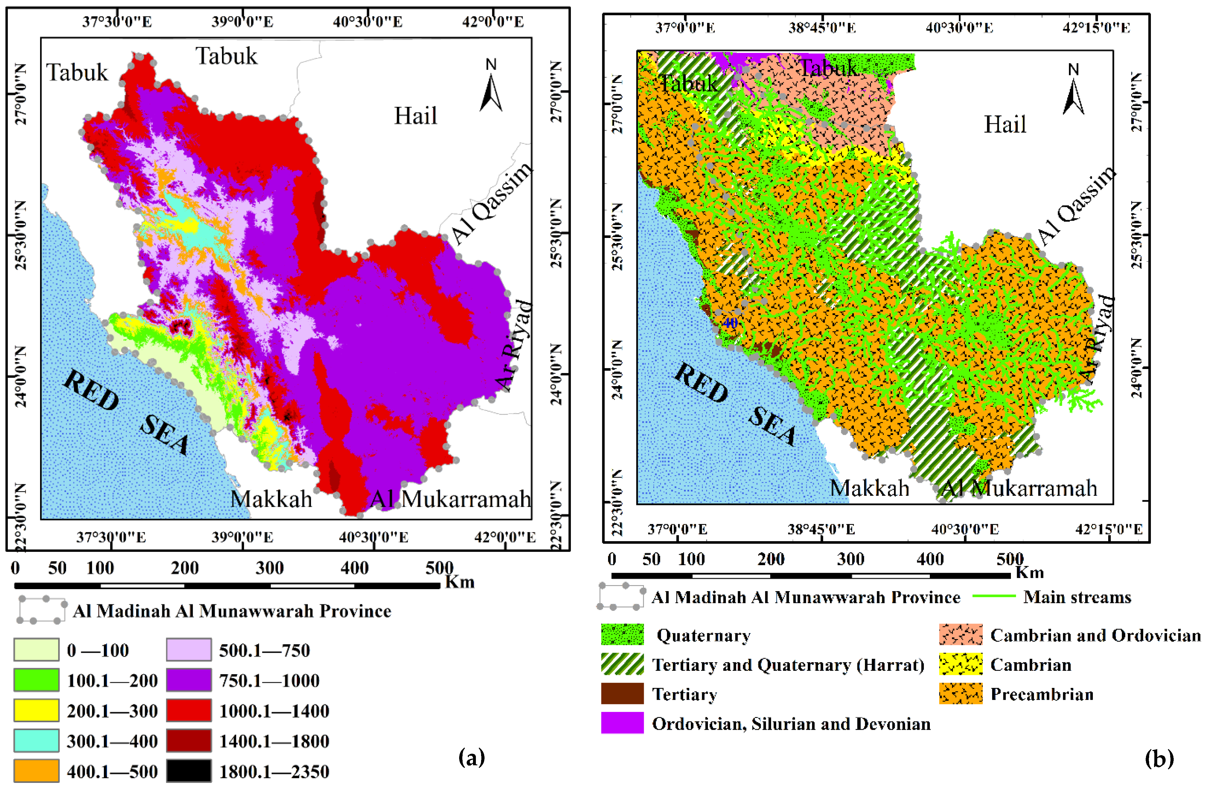
2.2. Geomorphology

Al Madinah Al Munawarah Province is located in the central part of the western zone of the KSA, with elevation ranges between 0 m at the Red Sea coastal line and about 2350 m at the Hijaz Mountains, as shown in Figure 4a. This portion comprises the coastal plain, foothills, and Hijaz Mountains as follows:

• The coastal plain (lowland areas) is located between the sabkhas alongside the Red Sea shoreline and the foothills, with widths varying from 20 km to 100 km. Usually, the lowland areas are inundated by flash floods along the major valleys of the drainage basins which are cross the Red Sea’s direction. This part is characterized by alluvial deposits which are suitable for groundwater recharge of the unconfined aquifers [35,36].
• The foothills (hilly areas) extend from the coastal plain to the mountainous range, with widths ranging between 60 km and 150 km and elevations about 400 m above mean sea level. This area is gently sloping and partly plateaus, and it is composed of boulders and alluvial deposits which are characterized by high permeability for water infiltration and aquifer recharge. Most of the stream networks originate from the Hijaz mountainous series crossing the hilly areas to the coastal plain.
• The Hijaz Mountains (highland areas) extend east from the hilly areas parallel to the Red Sea and are characterized by sharply high elevations that reach 3000 m. The stream networks are initiated from these highland areas and cross toward the lowland areas. Many hydrologic basins are located in the study province, which is called a coastal basin, and draining their water toward the Red Sea.

2.3. Geology

Geology plays a very important factor and has a direct impact on surface and groundwater by controlling the hydrological performance of the drainage basins, such as through the basin form, stream order, flashflood flow direction, and groundwater recharge of the unconfined aquifers.

Al Madinah Al Munawarah Province is located in the western part of the KSA (Arabian Shield), which belongs to the eastern boundary of the Red Sea rift. The Red Sea rift was initiated in the Oligocene and sustained into the Holocene age. Precambrian rocks outcrop alongside the northeastern edge of the Red Sea. The Al Madinah Al Munawarah plain is characterized by the presence of several volcanic intrusions and dikes that have occurred through the progress of the Red Sea rift. Figure 4b shows the geology of the study province.

The most important characteristic of Al Madinah Al Munawarah Province from a geological point of view is the presence of the volcanic Harrats, which represent about 20% of the study area and are distributed in many places (the south, north, northwest, west, and east). The Harrats are dark-colored basaltic rocks that were formed as a result of the eruption of lava from the ground to the surface during the Tertiary and Quaternary eras.

Additionally, the quaternary deposits represent about 13% of the study province and are considered the main shallow aquifer of the study area. These deposits are composed of boulders, gravels, and sands and are intercalated with some shales.

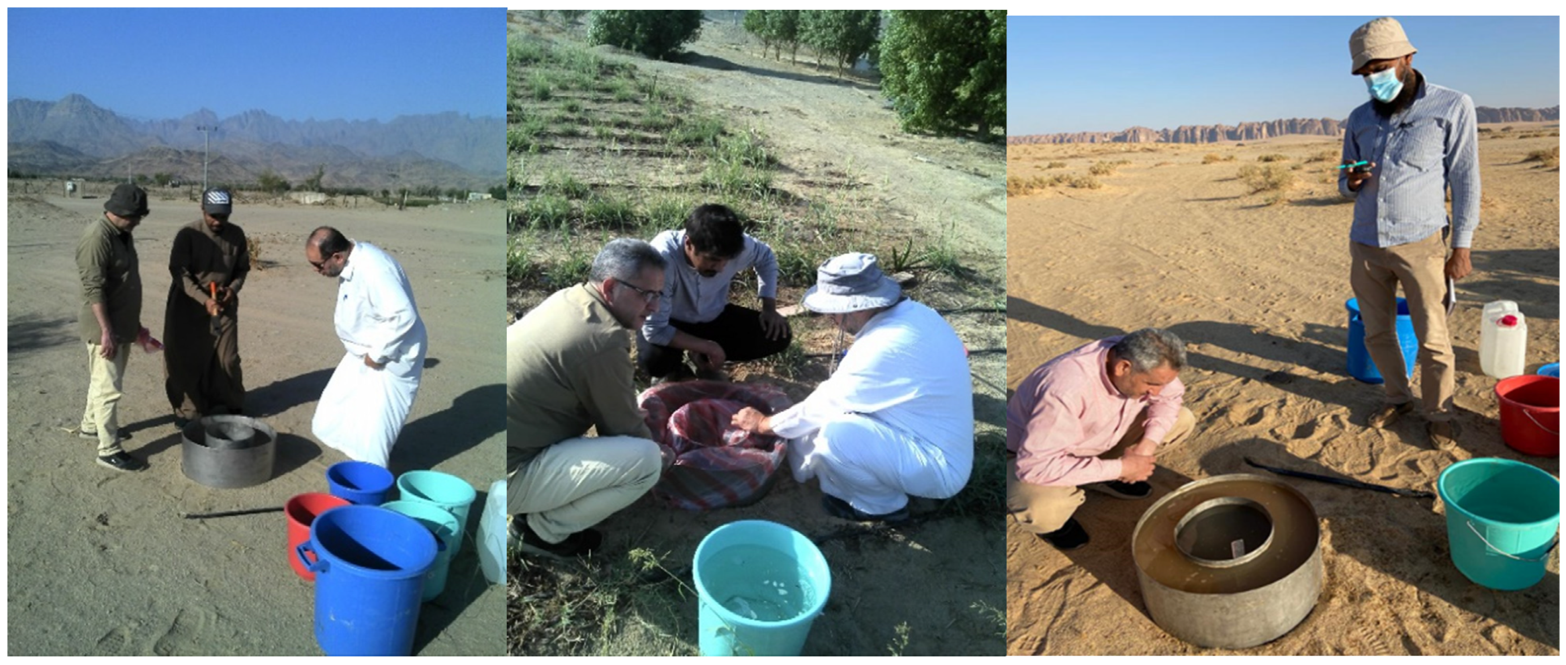
2.4. Infiltration Tests

The locations of the infiltration tests in this study are displayed in Figure 5. They covered Al Madinah Al Munawarah Province as shown in the figure. The locations of these tests were mainly in the alluvium, the ephemeral streams that help in understanding the infiltration characteristics for flash floods and consequently the transmission losses. Figure 6 shows the field measurements of the 14 tests in the study area. The figure shows high variability in the infiltration behavior that will be discussed in the following sections.

3. Methodology

3.1. Field Infiltration Tests

Double-ring infiltrometers are widely used for infiltration testing all over the world. According to [37,38], the infiltration tests in the study area were conducted using a double-ring infiltrometer. There are basic tools that must be present to conduct infiltration tests, and they are as follows: double rings (outer and inner), a rod of wood, a hammer for pushing down the rings into the soil, water buckets, a ruler for measuring the infiltrated water from the inner ring, and a stopwatch for controlling the time of infiltration.

The infiltrometers were composed of two rings 25 and 50 cm in diameter, with a ruler scale implanted into the soil about 10 cm using calm shocks by hammering without any turbulences or fluctuations in the soil structures, as shown in Figure 7. A constant water level was kept inside the infiltrometer. The external ring played a crucial role in preventing horizontal water seepage from the inner ring, allowing cylindrical flow through the inner ring. The infiltration test continued by water percolating into the soil over time, recording measurements until an approximate constant infiltration rate was reached.

3.2. Infiltration Models Used in the Analysis

Famous infiltration models were used to fit the infiltration data, namely the Philip [39], Horton [11,12], Kostiakov [13], and Green and Ampt [10] models. The equations used for these models are given in the following subsection.

3.2.1. Philip Model

The Philip infiltration equation is expressed as

$$f\left(t\right)=\frac{S}{2\sqrt{t}}+K_P$$

(2)

where f(t) is the infiltration rate at the time t, S is the soil sorptivity, K_P is the hydraulic conductivity of the soil, and t is the time since infiltration started.

The Philip cumulative infiltration depth F(t) is given by

$$F\left(t\right)=S\sqrt{t}+K_{P}t$$

(3)

The method of least squares (MLS) is formulated by the following objective function, which needs to be minimized to obtain the fitting parameters S and K_P:

$$Obj\left(S,K_P\right)=\min {{\displaystyle \sum }}_{i=1}^n{\left(\widehat{F}\left(t_i\right)-\left[S\sqrt{t_i}+K_P{t}_i\right]\right)}^2$$

(4)

where $\widehat{F}\left(t_i\right)$ is the observed cumulative infiltration (cm), t_i is the time corresponding to the observed cumulative infiltration (min), and n is the number of observations.

3.2.2. Horton Model

The Horton infiltration equation was also tested for fitting the infiltration data. The Horton model is given by

$$f\left(t\right)=f_c+\left(f_o-f_c\right)e^{-kt}$$

(5)

where f_o is the initial infiltration rate, f_c is the ultimate infiltration rate (equilibrium infiltration rate after the soil has been saturated), and k is the decay coefficient.

The Horton cumulative infiltration depth F(t) is given by

$$F\left(t\right)=f_{c}t+\frac{\left(f_o-f_c\right)}{k}\left(1-e^{-kt}\right)$$

(6)

The equation is fitted to the infiltration test data, and the parameters f_o, f_c, and k are estimated using the MLS. A similar formalism can be made as in Equation (4) to read

$$Obj\left(f_o,f_c,k\right)=\min {\displaystyle \sum }_{i=1}^n{\left(\widehat{F}\left(t_i\right)-\left[f_c{t}_i+\frac{\left(f_o-f_c\right)}{k}\left(1-e^{-k{t}_i}\right)\right]\right)}^2$$

(7)

3.2.3. Kostiakov Model

The Kostiakov infiltration equation is given by

$$f\left(t\right)=a{t}^b$$

(8)

where a and b are the model parameters.

The Kostiakov cumulative infiltration depth F(t) is the integration of the above equation, yielding

$$F\left(t\right)=\frac{a}{b+1}{t}^{b+1}$$

(9)

By fitting Equation (9) to the field test data, the parameters a and b can be estimated using the LSM. A similar formalism can be made as in Equation (4) to read

$$Obj\left(a,b\right)=\min {\displaystyle \sum }_{i=1}^n{\left(\widehat{F}\left(t_i\right)-\left[\frac{a}{b+1}{t}_i^{b+1}\right]\right)}^2$$

(10)

3.2.4. Green and Ampt Model

The Green and Ampt infiltration equation is given by

$$f\left(t\right)=K_S\left[1+\frac{\psi \Delta \mathsf{\theta }}{F\left(t\right)}\right]$$

(11)

where K_s is the saturated hydraulic conductivity of the soil, $\psi$ is the matric potential, $\Delta \mathsf{\theta }$ is the change in volumetric water content from the initial water content to the porosity, and F(t) is the cumulative infiltration depth.

The Green and Ampt cumulative infiltration depth F(t) is given by

$$F\left(t\right)=K_{S}t+\psi \Delta \mathsf{\theta }\ln \left[1+\frac{F\left(t\right)}{\psi \Delta \mathsf{\theta }}\right]$$

(12)

Equation (12) is fitted to the infiltration test data, and the parameters K_s, $\psi$, and $\Delta \mathsf{\theta }$ are estimated using the MLS. A similar formalism can be made as in Equation (4) to read

$$Obj\left(K_S, \psi ,\Delta \mathsf{\theta }\right)=\min {\displaystyle \sum }_{i=1}^n{\left(\widehat{F}\left(t_i\right)-\left[K_S{t}_i+\psi \Delta \mathsf{\theta }\ln \left(1+\frac{F\left(t\right)}{\psi \Delta \mathsf{\theta }}\right)\right]\right)}^2$$

(13)

The authors used a ready-made routine in Excel software for solving the optimization of the objective functions based on the gradient method, and the solution was performed several times until conversion to the optimized solution was achieved. Therefore, the parameters were estimated based on minimizing the objective function.

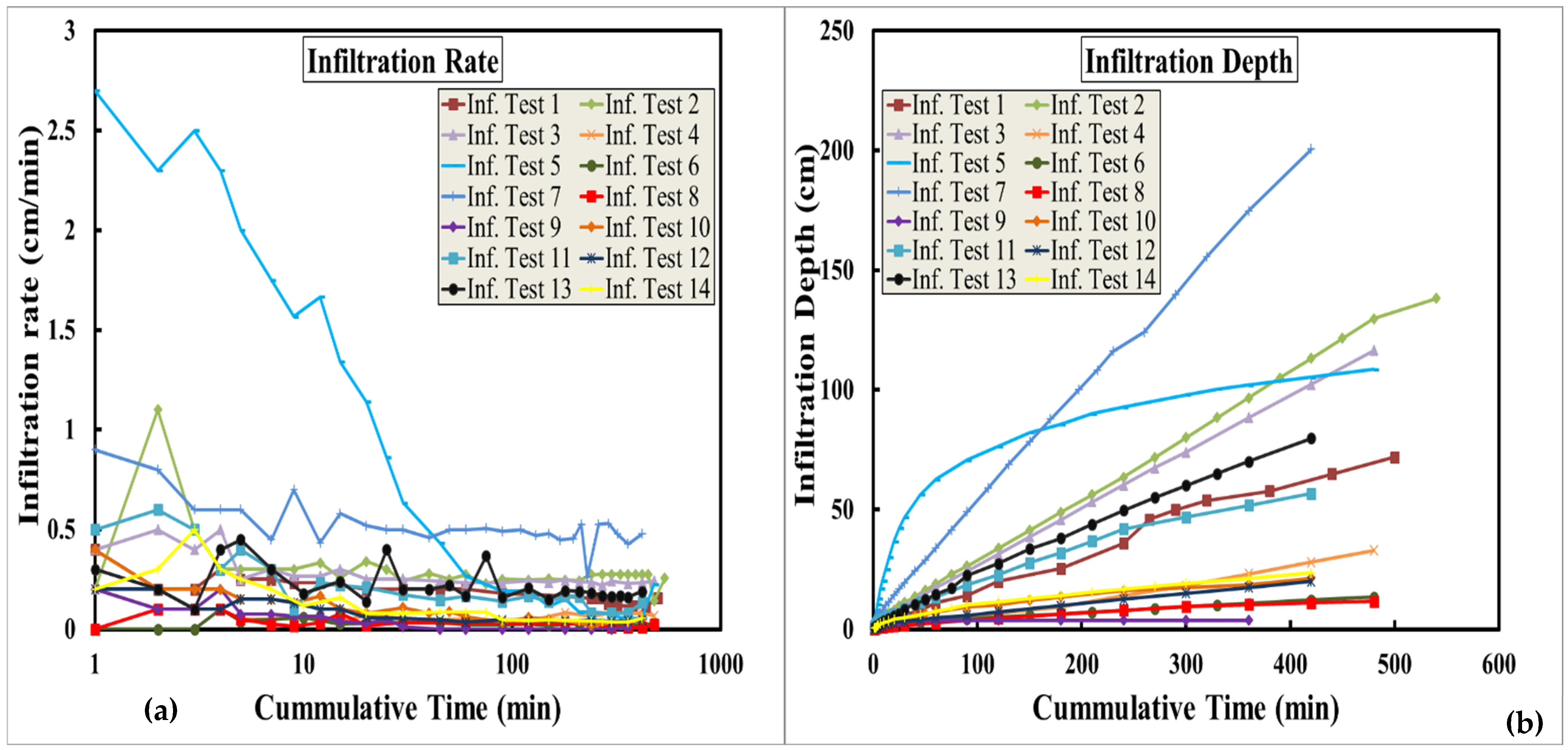
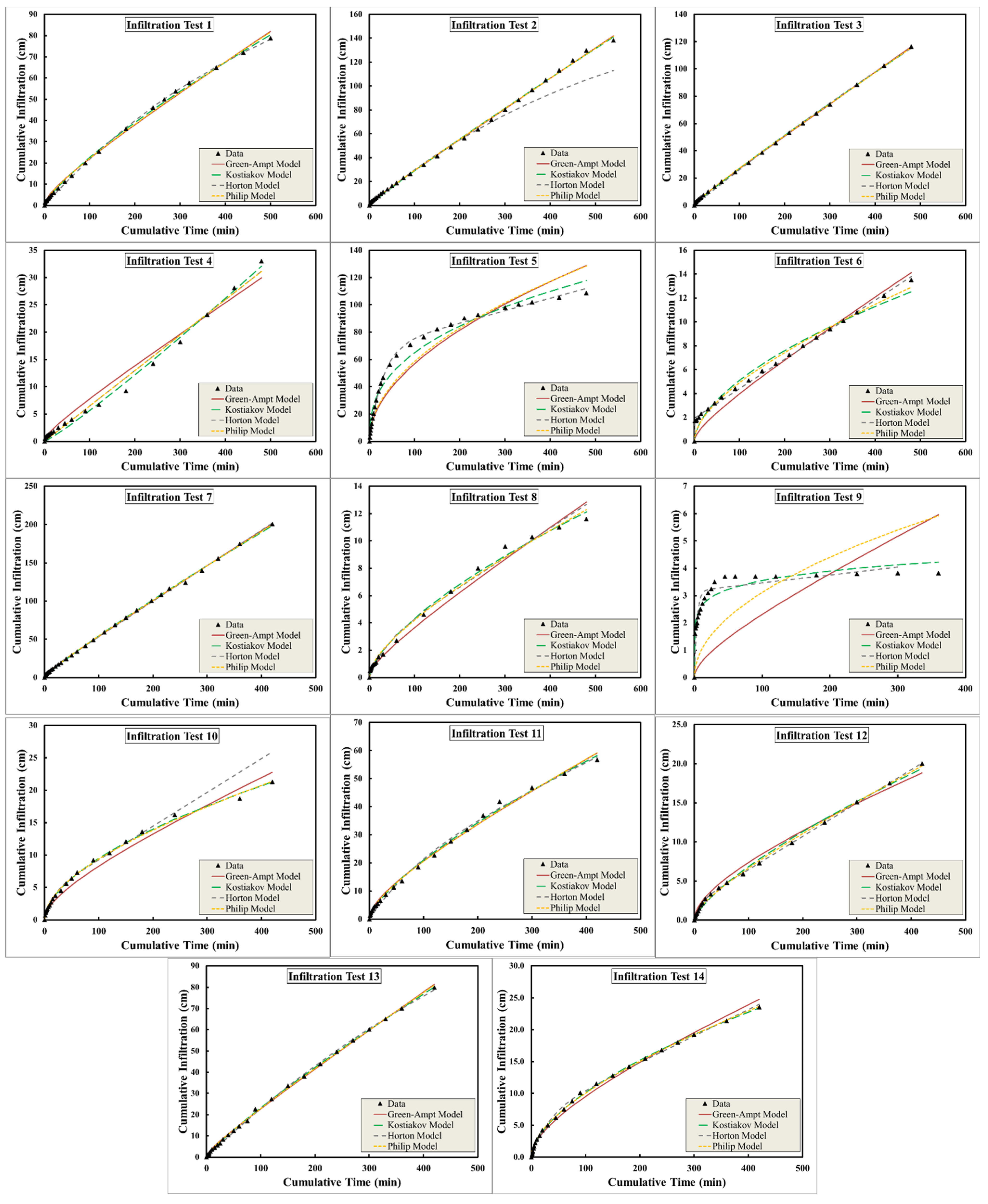
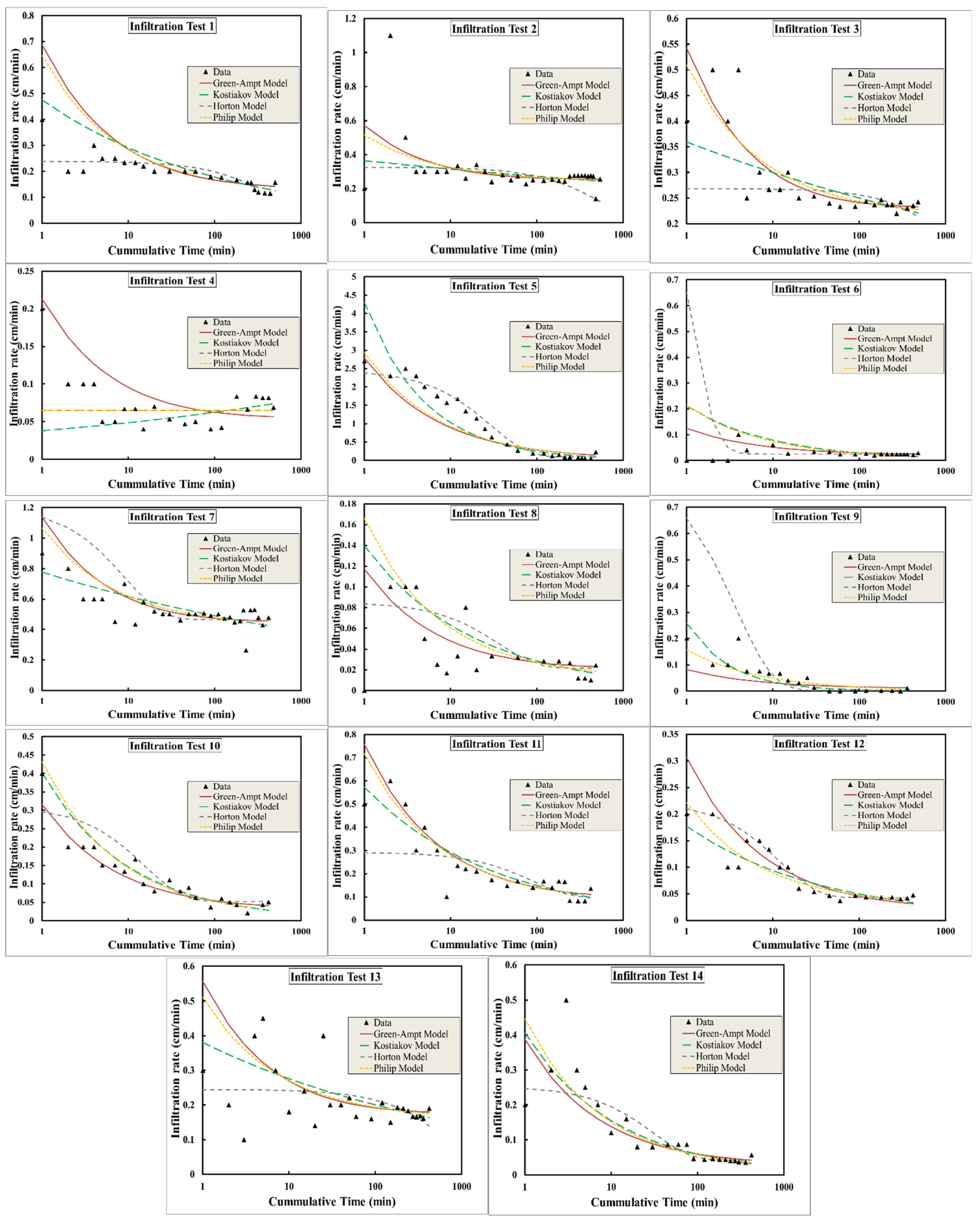
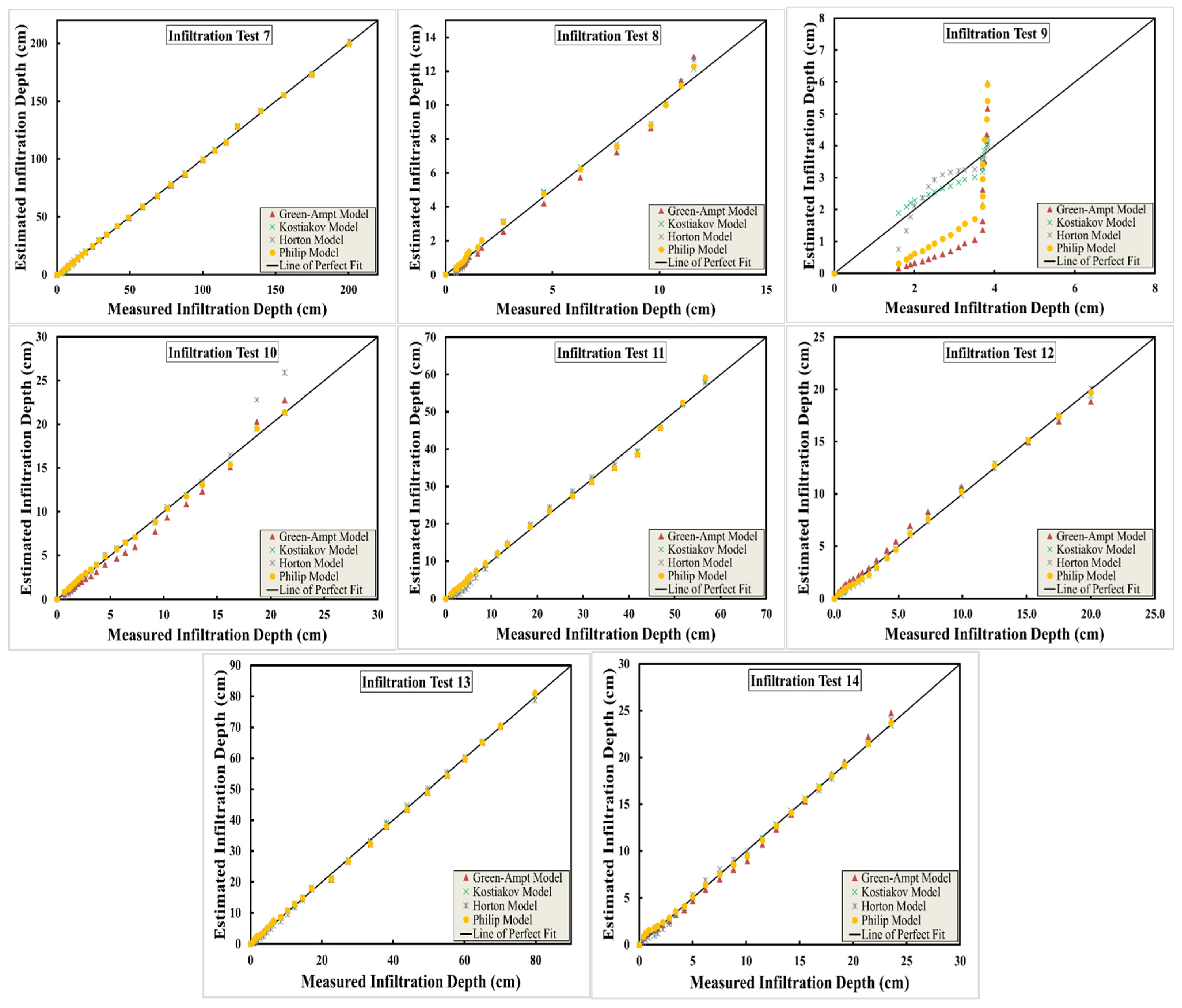
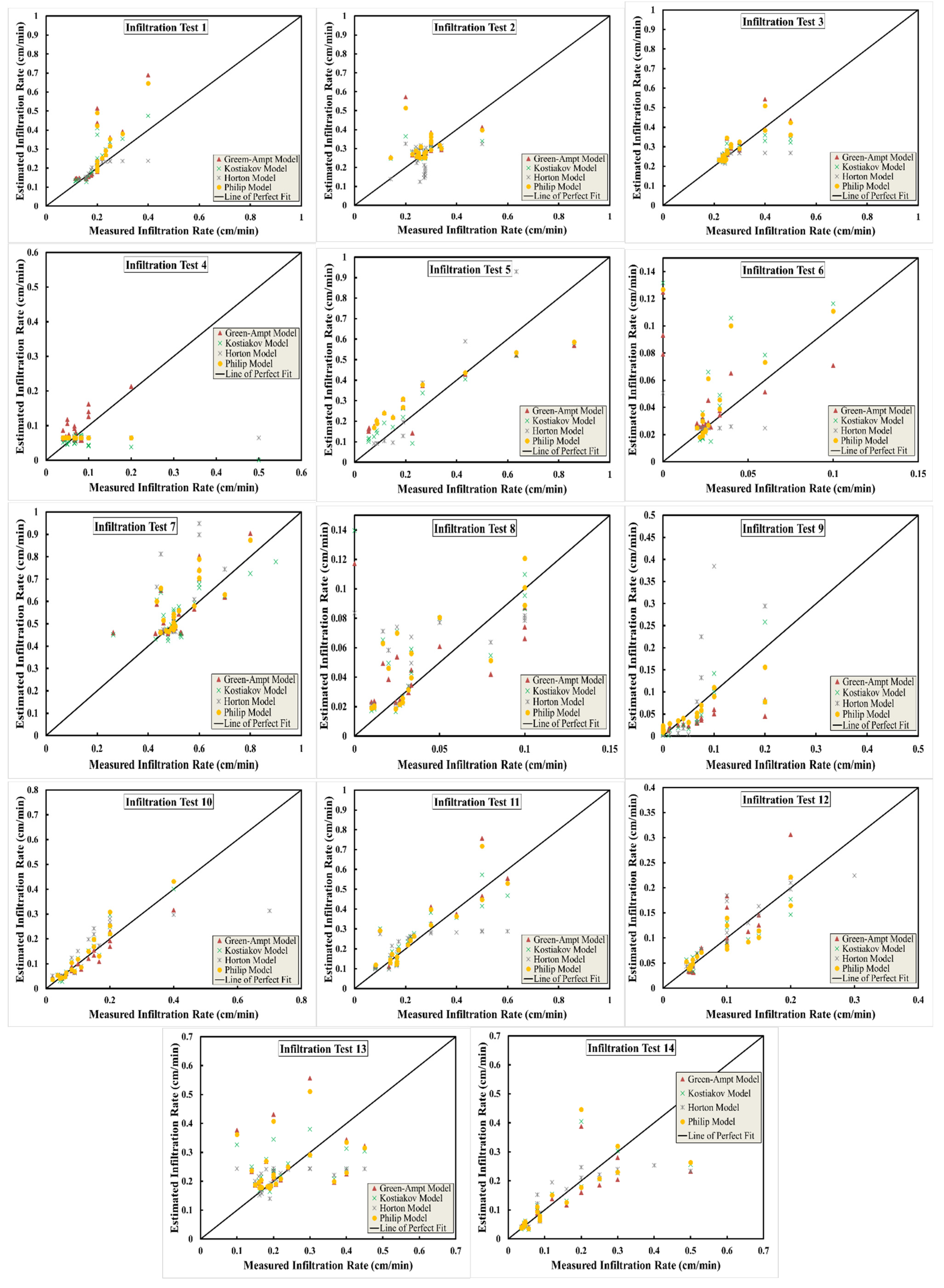
4. Results and Discussions

4.1. Comparison of the Various Infiltration Models

Figure 8 and Figure 9 display a comparison between the fitted and measured infiltration depths (Figure 8) and the measured infiltration rates (Figure 9) based on the four infiltration models used. The general overview shows that the infiltrated depth was fitted better to the models in comparison with the infiltration rates. The reason for that is the infiltrated depth is an integration of the infiltration rates, and therefore the presentation showed a better fit to the data. The high variability in the infiltration rates concerning the models is also obvious, which is an indication of the high variability in the soil characteristics in the test location (inherent variability) and between the locations (spatial variability), which seems to be typical for the region.

The majority of the tests showed agreement between the measured and infiltration equations in terms of infiltration depth. They showed the same behavior with different degrees of agreement with the measured data. Tests 5 and 9 showed the highest discrepancies between the model fitting and the measurements. Both tests showed the same behavior, where the waterfront progressed quickly early, while at the late time it progressed slowly. The reason for this behavior could be because, in the early time, two mechanisms (gravity and capillarity) were both acting downward, letting the water infiltrate quickly into the soil while at a later time, when the amount of water increased, the gravity dominated, and if there was a water table near the ground’s surface, the waterfront ceased to proceed down and touch the water table. Consequently, there would be a rise of the water table.

Table 1. Parameters of the infiltration models with summary statistics.

Inf. Test No.	Horton			Philip		Kostiakov		Green-Ampt		Mean (K, cm/min)	SD (K, cm/min)	CV (K)	Max (K, cm/min)	Min (K, cm/min)
	fc (cm/min)	fo (cm/min)	k (min−1)	S (cm/min.5)	Kp (cm/min)	a (cm/min b)	b	Ks (cm/min)	Ψ∆θ (cm)
1	0.002	0.239	0.002	1.06	0.116	0.787	8.69	0.134	5.308	0.308	0.343	0.90	0.787	0.00200
2	0.003	0.326	0.002	0.552	0.238	0.389	0.94	0.253	1.21	0.215	0.160	1.34	0.389	0.00300
3	0.00026	0.269	0.00047	0.591	0.214	0.39	0.92	0.231	1.241	0.207	0.160	1.29	0.390	0.00026
4	0.00027	0.065	0.000001	0	0.065	0.034	1.10	0.055	1.127	0.030	0.023	1.32	0.055	0.00027
5	0.091	2.463	0.035	5.86	0	11.398	0.38	0.023	680.1	3.837	5.346	0.72	11.398	0.02300
6	0.025	3.11	1.594	0.411	0.008	0.371	0.57	0.024	0.985	0.140	0.163	0.86	0.371	0.02400
7	0.465	1.216	0.11	1.307	0.412	0.864	0.9	0.449	2.989	0.593	0.192	3.09	0.864	0.44900
8	0.022	0.085	0.027	0.309	0.012	0.213	0.65	0.021	0.986	0.085	0.090	0.95	0.213	0.02100
9	0.003	0.863	0.271	0.312	0	1.897	0.14	0.011	0.981	0.637	0.891	0.71	1.897	0.00300
10	0.052	0.313	0.064	0.843	0.009	0.713	0.56	0.033	5.12	0.266	0.316	0.84	0.713	0.03300
11	0.095	0.293	0.011	1.278	0.078	0.81	0.71	0.094	10.221	0.333	0.337	0.99	0.810	0.09400
12	0.042	0.225	0.082	0.387	0.029	0.245	0.72	0.022	7.622	0.103	0.101	1.02	0.245	0.02200
13	0.002	0.245	0.001	0.704	0.159	0.441	0.86	0.175	2.16	0.206	0.181	1.14	0.441	0.00200
14	0.041	0.254	0.032	0.864	0.014	0.697	0.58	0.031	8.609	0.256	0.312	0.82	0.697	0.03100
Max	0.47	3.11	1.59	5.86	0.41	11.40	8.69	0.45	680.06	3.84	5.35	3.09	11.40	0.45
Min	0.00026	0.07	0.000001	0.00	0.00	0.03	0.14	0.01	0.98	0.03	0.02	0.71	0.06	0.00026
Mean	0.06	0.71	0.16	1.03	0.10	1.37	1.27	0.11	52.04	0.52	0.62	1.14	1.38	0.05
SD	0.12	0.91	0.40	1.39	0.12	2.81	2.07	0.12	174.21	0.94	1.33	0.58	2.81	0.11
CV	1.93	1.27	2.53	1.34	1.21	2.05	1.64	1.10	3.35	1.82	2.16	0.50	2.04	2.24

Max = maximum value of the parameter; Min = minimum value of the parameter; Mean = mean value of the parameter; SD = standard deviation; CV = coefficient of variation.

shows the parameters of each model.

For the Horton model (a three-parameter model: f_o, f_c, and k), fo varied between 3.11 cm/min and 0.07 cm/min with CV = 1.27. The results indicate high variability in the initial infiltration rates f_o. Most of the tests showed relatively moderate values, except Test 4, which had the lowest value. This lowest value could be interpreted as the soil having fine sediments that impeded the water’s flow downward. The final infiltration capacity, f_c, corresponding to the saturated hydraulic conductivity in the vertical direction of the surface soil, varied between 0.47 cm/min and 0.00026 cm/min with CV = 1.93. Again, high variability was observed in f_c, indicating different soil types in these wadi beds. Moreover, the variability in f_c was higher than the variability in f_o. This is an indication of the variability in the hydraulic characteristics of the soil profile. The decay parameter k is an indication of how fast or slow the infiltration process is. The decay k was extremely variable (CV = 2.43), where the extreme minimum value was 10⁻⁷ min⁻¹ (very slow infiltration in Test 4) while the minimum was 0.00047 (slow infiltration), and the extreme maximum value was 1.59 min⁻¹ (very fast infiltration in Test 6) while the maximum value was 0.271 min⁻¹ (fast infiltration). Excluding the extreme values, the variability in the decay parameter dropped to CV = 1.39.

For the Philip model (a two-parameter model: S and K_p), the value of S varied between 0 and 5.86 cm/min^0.5 with CV = 1.34. The minimum nonzero value was 0.309 cm/min^0.5. The zero value of S was also reported in the recent study by [40]. This indicates that full saturation of the soil was reached during the experiment (Test 4). This result was confirmed by the Horton model, where k = 10⁻⁷ min⁻¹ (very slow infiltration in Test 4), which means a high degree of soil saturation. The value of K_p, which is a representation of the saturated hydraulic conductivity, varied between 0 and 0.41 cm/min with CV = 1.21. The minimum nonzero value was 0.009 cm/min. When the zero values were removed, the CV reduced to 1.05.

The comparison between the saturated hydraulic conductivity estimated by the Horton model f_c and K_p from the Philip model showed discrepancies due to the basic background between the two models. The Horton model has an empirical one, but the Philip model is a physically based model. The CV of f_c (1.93) was higher than the CV of K_p (1.05). This indicates that f_c is more highly variable than K_p. The reason for this can be because the Horton model has a three-parameter space to search for the optimum solution values, which can lead to high variability in the parameters, while the Philip model has a two-parameter space to search for the optimum solution so that it is more restricted and leads to less variability. The zero values of K_p at Tests 5 and 9 could be attributed to a thin impermeable layer that is encountered during the process of infiltration and does not allow the process to continue. This is obvious in Figure 9 (Tests 5 and 9), where the cumulative infiltration depth levels off at a later time.

For the Kostiakov model (a two empirical parameter model: a and b), the coefficient parameter a varied between 0.03 and 11.4 with CV = 2.05. Meanwhile, the exponent parameter b varied between 0.14 and 8.69 with CV = 1.64. The parameters still showed high variability in the range of availability of the physical parameters of other models, while this model seemed to be more flexible to fit the data and provide nonzero values for both parameters. Nevertheless, these parameters are empirical and have no physical interpretation.

For the Green and Ampt model (a quasi-two physical parameter model: K_s and $\left(\psi \Delta \mathsf{\theta }\right),$ the saturated hydraulic conductivity K_s varied between 0.01 and 0.45 cm/min with CV = 1.1. The value of the CV of K_s was in agreement with the CV of K_p in the Philip model after excluding the zeros (1.05). This at least shows coherence between the two models. The parameter $\left(\psi \Delta \mathsf{\theta }\right)$ is the multiplication of the matric head and the change in the volumetric water content. It varied between 0.98 cm and 680.06 cm (Test 5) with CV = 3.35. This is very high variability. This test showed the highest initial infiltration among all tests (3.11 cm/min). It indicated the high dryness of the soil, and that the capillarity was very significant, which appeared in the figure. However, the maximum value seems to be an outlier. The lower value below the maximum was 10.2 cm, which looks reasonable, and removing the outlier would lead the CV to reach 0.85.

Since saturated hydraulic conductivity is one of the significant parameters in the infiltration process, we therefore will elaborate on its analysis. In Table 1 (the last five columns), we studied the statistics of the saturated hydraulic conductivity estimated from three models (Horton (f_c), Philip (K_p), and Green–Ampt, (K_s)). The average value, the standard deviation (SD), the CV, and the minimum and maximum were calculated for each test and all tests overall. The results show that there was variability of the mean K for the overall tests, with a minimum K = 0.03 cm/min (Test 4), a maximum K = 3.84 cm/min (Test 5), and CV(K) = 1.82, which indicates high variability in the overall mean hydraulic conductivity between the tests. The SD (K) varied between the tests and had a minimum value of 0.02 cm/min (Test 4) and a maximum value of 5.35 cm/min (Test 5) with CV = 2.16. The minimum CV between the tests was 0.71 (Test 9), and the maximum CV was 3.09 (Test 7). The maximum of the maximum values between the tests was 11.4 cm/min (Test 5), while the minimum of the maximum values between the tests was 0.06 cm/min (Test 4). The maximum of the minimum values between the tests was 0.45 cm/min (Test 7), while the minimum of the minimum values between the tests was 0.00026 cm/min (Test 3).

From the aforementioned analysis, one may conclude the following:

There is variability in the various models for estimating the saturated hydraulic conductivity. This could be due to the theoretical background of each model.

Tests 3, 4, 5, 7, and 9 among the 14 tests showed the highest variability in terms of extreme values in the saturated hydraulic conductivity statistics.

4.2. Estimated Versus Measured Infiltration Depths and Rates

Figure 10 and Figure 11 show a plot between the estimated and measured infiltration depths and rates, respectively. The comparison shows the estimated infiltration based on the four models that appeared with symbols in the figures, and the line of perfect fit is presented. Statistical measures of the model performance are displayed in

Table 2. Statistical measures of the performance of the infiltration models.

Inf. Test No.	Horton				Philip				Kostiakov				Green-Ampt				Max R and Min RMSE				Best Model
	f (cm/min)		F (cm)		f (cm/min)		F (cm)		f (cm/min)		F (cm)		f (cm/min)		F (cm)		f (cm/min)		F (cm)
	R	RMSE	R	RMSE	R	RMSE	R	RMSE	R	RMSE	R	RMSE	R	RMSE	R	RMSE	R	RMSE	R	RMSE
1	0.319	0.263	0.999	0.936	0.718	0.096	0.998	1.210	0.850	0.060	0.990	0.790	0.830	0.107	0.990	1.330	0.850	0.060	0.999	0.790	Kostiakov
2	0.294	0.178	0.994	8.680	0.468	0.157	0.999	1.390	0.452	0.164	0.999	1.674	0.460	0.157	0.999	1.288	0.468	0.157	0.999	1.288	Philip/Green-Ampt
3	0.325	0.079	1.000	1.401	0.816	0.047	1.000	0.563	0.775	0.056	1.000	1.020	0.811	0.049	0.999	0.411	0.816	0.047	1.000	0.411	Philip
4	0.156	0.034	0.995	0.951	0.000	0.034	0.995	0.951	−0.781	0.042	0.998	0.803	0.732	0.032	0.991	1.399	0.732	0.032	0.998	0.803	Kostiakov/Green-Ampt
5	0.984	0.165	0.999	1.684	0.922	0.450	0.973	9.986	0.898	0.457	0.987	6.374	0.932	0.442	0.968	10.751	0.984	0.165	0.999	1.684	Horton
6	0.973	0.144	0.999	0.184	−0.107	0.064	0.993	0.566	−0.080	0.064	0.989	0.647	−0.119	0.038	0.997	0.853	0.973	0.038	0.999	0.184	Horton
7	0.623	0.171	1.000	1.416	0.868	0.088	1.000	1.154	0.738	0.089	0.999	1.706	0.830	0.106	0.999	1.122	0.868	0.088	1.000	1.122	Philip
8	0.420	0.030	0.996	0.441	0.394	0.042	0.997	0.316	0.448	0.037	0.994	0.281	0.384	0.032	0.995	0.479	0.448	0.030	0.997	0.281	Kostiakov
9	0.753	0.153	0.953	0.318	0.892	0.031	0.774	1.445	0.842	0.034	0.961	0.281	0.890	0.050	0.744	1.830	0.892	0.031	0.961	0.281	Kostiakov/Philip
10	0.770	0.047	0.992	1.378	0.960	0.032	0.998	0.352	0.958	0.030	0.999	0.280	0.962	0.027	0.993	0.916	0.962	0.027	0.999	0.280	Kostiakov/Green-Ampt
11	0.591	0.105	0.998	1.329	0.885	0.070	0.998	1.113	0.893	0.063	0.999	0.941	0.897	0.076	0.998	1.180	0.897	0.063	0.999	0.941	Kostiakov
12	0.900	0.025	1.000	0.066	0.899	0.022	0.999	0.220	0.910	0.023	0.993	0.360	0.901	0.035	0.998	0.574	0.910	0.022	1.000	0.066	Horton
13	0.403	0.085	0.785	1.000	0.339	0.104	0.999	0.673	0.405	0.088	0.999	0.448	0.320	0.111	0.999	0.801	0.405	0.085	0.999	0.448	Kostiakov
14	0.858	0.063	0.999	0.352	0.774	0.073	0.999	0.299	0.795	0.069	1.000	0.215	0.773	0.073	0.998	0.541	0.858	0.063	1.000	0.215	Horton
Max	0.98	0.26	1.00	8.68	0.96	0.45	1.00	9.99	0.96	0.46	1.00	6.37	0.96	0.44	1.00	10.75
Min	0.16	0.03	0.79	0.07	−0.11	0.02	0.77	0.22	−0.78	0.02	0.96	0.22	−0.12	0.03	0.74	0.41
Mean	0.60	0.11	0.98	1.44	0.63	0.09	0.98	1.45	0.58	0.09	0.99	1.13	0.69	0.10	0.98	1.68
SD	0.27	0.07	0.06	2.07	0.34	0.10	0.06	2.40	0.47	0.11	0.01	1.53	0.30	0.10	0.06	2.55
CV	0.45	0.62	0.06	1.44	0.54	1.12	0.06	1.66	0.81	1.17	0.01	1.35	0.44	1.08	0.07	1.52

R = correlation coefficient between measured and estimated f and F; RMSE = root mean square error between measured and estimated f and F; Max = maximum value of the coefficient; Min = minimum value of the coefficient; Mean = mean value, SD = standard deviation; CV = coefficient of variation. The boldfaced numbers are the max R for both f and F. The boldfaced italicized numbers are the minimum RMSE for both f and F.

. The table shows two statistical measures—the correlation coefficient between the measured and estimated infiltration rates and depths (R) and the root means square error (RMSE) for every test—and the overall statistics of the measures (minimum, maximum, mean, standard deviation, and CV) for both R and RMSE as well as for both the infiltration rates f and infiltration depths F, respectively. R shows how strong or weak the relation between the measured and estimated infiltration is, and RMSE shows the average error in the estimation. The last four columns in Table 2 show the maximum R and the minimum RMSE for both f and F, respectively. The boldfaced numbers in the table show the corresponding model with the maximum R, while the boldfaced italicized numbers show the corresponding model with the minimum RMSE. The fifth column shows the best model based on R and RMSE.

For the Horton model, R varied between 0.16 (Test 6) and 0.98 (Test 5) with CV = 0.45 for f. The majority of the tests showed high correlation, except for Test 6, which showed the lowest correlation. For F, R varied between 0.79 (Test 13) and 1 (Tests 3, 7, and 12) with CV = 0.06, showing quite low variability. The R for F was always higher than the R for f, and this was due to the integration of f to obtain F (i.e., the accumulation of f improved the correlation R). Regarding the accuracy of the model, the RMSE was estimated. The RMSE varied between 0.025 (Test 12) and 0.26 cm/min (Test 1) for f with CV = 0.62, showing moderate variability. Meanwhile, for F, the RMSE varied between 0.07 (Test 12) and 8.68 cm (Test 2) with CV = 1.44, showing relatively high variability.

For the Philip model, R varied between −0.11 (Test 6) and 0.96 (Test 10) with CV = 0.54 for f, and the majority of the tests showed high correlation, except for Test 6, which showed a low and negative correlation. Test 4 had no correlation, since the data in these tests did not show a regular pattern with an indication of soil heterogeneity in the site of the tests (see Figure 10, Tests 4 and 6). For F, R varied between 0.77 (Test 9) and 1 (Tests 3 and 7) with CV = 0.06, showing quite low variability. The RMSE varied between 0.02 (Test 12) and 0.45 cm/min (Test 5) for f with CV = 1.12, showing high variability. Meanwhile, for F, the RMSE varied between 0.22 cm (Test 12) and 9.9 cm (Test 5) with CV = 1.66, showing high variability.

For the Kostiakov model, R varied between −0.34 (Test 4) and 0.96 (Test 10) with CV = 0.63 for f. The majority of the tests showed high correlation, except for Test 4, which showed low and negative correlation similar to Philip’s model, as mentioned in the above paragraph (see Figure 10, Test 4). For F, R varied between 0.96 (Test 9) and 1 (Tests 3 and 14) with CV = 0.01, which showed very low variability. The RMSE varied between 0.02 (Test 12) and 0.46 cm/min (Test 5) for f with CV = 1.17, showing high variability. Meanwhile, for F, the RMSE varied between 0.22 cm (Test 14) and 6.37 cm (Test 5) with CV = 1.35, showing high variability. The overall results of the Kostiakov model had great similarities with the Philip model in terms of R and RMSE. Although they are from different backgrounds, the first is an empirical model, while the last is a physically based model.

For the Green–Ampt model, R varied between −0.12 (Test 6) and 0.96 (Test 10) with CV = 0.44 for f. The majority of the tests showed relatively high correlation, except for Test 6, which showed a low and negative correlation. For F, R varied between 0.74 (Test 9) and 0.999 (Tests 2 and 13) with CV = 0.07, which showed low variability. The RMSE varied between 0.03 (Test 4) and 0.44 cm/min (Test 5) for f with CV = 1, showing high variability. Meanwhile, for F, the RMSE varied between 0.41 cm (Test 3) and 10.75 cm (Test 5) with CV = 1.52, showing high variability.

The overall results show that each test could be better presented by a specific model based on the maximum R and the minimum RMSE. The best fit could either be observed in f or F. The last column in Table 2 shows the best model for each test. The Kostiakov model seems to best fit most of the tests (7/14) (i.e., 50% of the tests), the Horton model represents 29%, the Philip model represents 14% and the Green–Ampt model represents 7%.

5. Conclusions and Recommendations

(1) The infiltration tests showed highly variable soil parameters. The initial infiltration rate f_o, based on the Horton model varied between 0.07 and 3.11 cm/min with CV = 1.27. The saturated hydraulic conductivity K obtained from the 3 infiltration models (Horton (f_c), Philip (K_p), and Green and Ampt (K_s)) and based on the 14 tests, on average, varied between 0.03 and 3.84 cm/min with CV = 1.82. The sorptivity coefficient S in the Philp equation, which reflects the matric properties of the soils, varied between almost 0.0 and 5.86 cm/min^0.5. The parameter $\left(\psi \Delta \mathsf{\theta }\right)$ in the Green and Ampt model varied between 0.98 cm and 10.2 cm after removing the outlier with CV = 0.85. These results imply significant variability in the groundwater recharge rates from flash floods in the region.

(2) The plots of the infiltration rate f demonstrated always having high variability in the tests when compared with the cumulative infiltration F. The reason for this is the integration of f to find F, where the accumulation of the values due to integration diminishes the high variability in f.

(3) Based on the comparison between the models’ performance, on average across the 14 tests, it has been shown that the Green and Ampt model had the highest R = 0.69 for f and R = 0.98 for F while having an RMSE = 0.1 cm/min for f and RMSE = 1.68 cm for F. Other models had lesser R values that varied between 0.57 and 0.63 for f but had R = 0.98 for F. In addition, the RMSE for f of all models was 0.1 cm/min. The minimum RMSE for F was 1.13 cm for the Kostiakov model, while other models varied between 1.44 and 1.68 cm. Therefore, the Kostiakov model seems to be the best model to represent these tests on average, since it had the minimum RMSE for F (1.13 cm) and had the same RMSE for f (0.1 cm/min) with acceptable R = 0.61 for f and R = 0.99 for F.

(4) The Kostiakov model best fit 50% of the tests, while the Horton model 29%, the Philip model fit 14%, and the Green–Ampt model fit 7%. The variability in the various models to estimate the saturated hydraulic conductivity could be due to the theoretical background of each model. Tests 3, 4, 5, 7, and 9 among the 14 tests showed the highest variability in terms of extreme values in the saturated hydraulic conductivity statistics.

For future work, it would be interesting to test other infiltration models different from the ones used in the current study. Additionally, applications of such models in different arid regions worldwide would provide generation of the current conclusions.

References

- Garg, S.; Goel, A. Infiltration—A Critical Review. In Sustainable Engineering; Springer: Berlin/Heidelberg, Germany, 2019; pp. 111–120. [Google Scholar]
- Elfeki, A.M.; Ewea, H.A.R.; Bahrawi, J.A.; Al-Amri, N.S. Incorporating transmission losses in flash flood routing in ephemeral streams by using the three-parameter Muskingum method. Arab. J. Geosci. 2014, 8, 5153–5165. [Google Scholar] [CrossRef]
- Richards, L.A. Capillary conduction through porous mediums. Physics 1931, 1, 313–318. [Google Scholar] [CrossRef]
- Rawls, W.J.; Ahuja, L.R.; Brakensiek, D.L.; Shirmohammadi, A. Infiltration and soil water movement. In Handbook of Hydrology; McGraw-Hill, Inc.: New York, NY, USA, 1993. [Google Scholar]
- Li, W.; Pang, Y. Application of Adomian decomposition method to nonlinear systems. Adv. Differ. Equ. 2020, 1, 67. [Google Scholar] [CrossRef]
- Turkyilmazoglu, M. Nonlinear Problems via a Convergence Accelerated Decomposition Method of Adomian. J. Comput. Model. Eng. Sci. 2021, 127, 1–22. [Google Scholar] [CrossRef]
- Turkyilmazoglu, M. Accelerating the convergence of Adomian decomposition method (ADM). J. Comput. Sci. 2019, 31, 54–59. [Google Scholar] [CrossRef]
- García-Olivares, A. Analytical solution of nonlinear partial differential equations of physics. Kybernetes 2003, 32, 548–560. [Google Scholar] [CrossRef] [Green Version]
- Philip, J.R. The theory of Infiltration. Soil. Sci. 1957, 83, 345–357. [Google Scholar] [CrossRef]
- Green, W.H.; Ampt, G.A. Studies in soil physics—Part 1: The flow of air and water through soils. J. Agric. Sci. 1911, 4, 1–24. [Google Scholar]
- Horton, R.E. The role of infiltration in the hydrological cycle. EOS Trans. Am. Geophys. Union 1933, 14, 446–460. [Google Scholar] [CrossRef]
- Horton, R.E. Analysis of runoff-plot experiments with varying infiltration capacity. EOS Trans. Am. Geophys. Union 1939, 20, 693–711. [Google Scholar] [CrossRef]
- Kostiakov, A.N. On the dynamics of the coefficients of water percolation in soils and on the necessity of studying it from a dynamic point of view for purpose of amelioration. Trans. 6th Commun. Int. Soc. Soil Sci. 1932, 1, 17–21. [Google Scholar]
- Allam, M.N.; Balkhair, K.S. Case study evaluation of the geomorphologic instantaneous unit hydrograph. Water Resour. Manag. 1987, 1, 267–291. [Google Scholar] [CrossRef]
- Noor, K.; Elfeki, A.M. Development of a generalized Hayami solution for modelling of a diffusive flood wave in arid and non-arid regions. Nat. Hazards 2017, 88, 121–144. [Google Scholar] [CrossRef]
- Hayami, S. On the propagation of flood waves. Bull.-Disaster Prev. Res. Inst. Kyoto Univ. 1951, 1, 1–16. [Google Scholar]
- Elfeki, A.; Masoud, M.; Basahi, J.; Zaidi, S. A unified approach for hydrological modeling of arid catchments for flood hazards assessment: Case study of wadi Itwad, southwest of Saudi Arabia. Arab. J. Geosci. 2020, 13, 490. [Google Scholar] [CrossRef]
- Schaap, M.G.; Leij, F.J. Using neural networks to predict soil water retention and soil hydraulic conductivity. Soil Tillage Res. 1998, 47, 37–42. [Google Scholar] [CrossRef]
- Erzin, Y.; Gumaste, S.D.; Gupta, A.K.; Singh, D.N. Artificial neural network (ANN) models for determining hydraulic conductivity of compacted fine-grained soils. Can. Geotech. J. 2009, 46, 955–968. [Google Scholar] [CrossRef]
- Arshad, R.R.; Sayyad, G.; Mosaddeghi, M.; Gharabaghi, B. Predicting saturated hydraulic conductivity by artificial intelligence and regression models. ISRN Soil Sci. 2013, 2013, 308159. [Google Scholar] [CrossRef] [Green Version]
- Al-Sulaiman, M.A.; Aboukarima, A.M. Distribution of natural radionuclides in the surface soil in some areas of agriculture and grazing located in west of Riyadh, Saudi Arabia. J. Appl. Life Sci. Int. 2015, 7, 1–12. [Google Scholar] [CrossRef]
- Saito, T.; Yasuda, H.; Suganuma, H.; Inosako, K.; Abe, Y.; Kojima, T. Predicting Soil Infiltration and Horizon Thickness for a Large-Scale Water Balance Model in an Arid Environment. Water 2016, 8, 96. [Google Scholar] [CrossRef] [Green Version]
- Singh, B.; Sihag, P.; Singh, K. Modelling of impact of water quality on infiltration rate of soil by random forest regression. Modeling Earth Syst. Environ. 2017, 3, 999–1004. [Google Scholar] [CrossRef]
- Sihag, P. Prediction of unsaturated hydraulic conductivity using fuzzy logic and artificial neural network. Modeling Earth Syst. Environ. 2018, 4, 189–198. [Google Scholar] [CrossRef]
- Masoud, M.H.Z.; Basahi, J.M.; Zaidi, F.K. Assessment of artificial groundwater recharge potential through estimation of permeability values from infiltration and aquifer tests in unconsolidated alluvial formations in coastal areas. Environ. Monit. Assess 2019, 191, 31. [Google Scholar] [CrossRef] [PubMed]
- Huang, J.; Wu, P.; Zhao, X. Effects of rainfall intensity, underlying surface and slope gradient on soil infiltration under simulated rainfall experiments. Catena 2013, 104, 93–102. [Google Scholar] [CrossRef]
- Liu, Y.; Cui, Z.; Huang, Z.; López-Vicente, M.; Wu, G. Influence of soil moisture and plant roots on the soil infiltration capacity at different stages in arid grasslands of China. Catena 2019, 182, 104147. [Google Scholar] [CrossRef]
- Cheng, Y.; Yang, W.; Zhan, H.; Jiang, O.; Shi, M.; Wang, Y. On the Origin of Deep Soil Water Infiltration in the Arid Sandy Region of China. Water 2020, 12, 2409. [Google Scholar] [CrossRef]
- Almazroui, M.A.; Al Khalaf, A.K.; Abdel Basset, H.M.; Hasanean, H.M. Detecting Climate Change Signals in Saudi Arabia Using Surface Temperature; King Abdelaziz University: Jeddah, Saudi Arabia, 2009. [Google Scholar]
- Köppen, W. Das Geographische System der Klimate. In Handbuch der Klimatologie; Köppen, W., Geiger, R., Eds.; Gebrüder Borntraeger: Berlin, Germany, 1936; pp. 1–44. [Google Scholar]
- Trewartha, G.T. An Introduction to Climate, 3rd ed.; McGraw-Hill: New York, NY, USA, 1954. [Google Scholar]
- Hevesi, J.; Flint, A.; Istok, J. Precipitation estimation in mountainous terrain using multivariate geostatistics: Part 1. J. Appl. Meteorol. Climatol. 1992, 31, 661–688. [Google Scholar] [CrossRef]
- Al-Turki, S. Water Resources in Saudi Arabia with Particular Reference to Tihama Asir Province. Ph.D. Thesis, University of Durham, Durham, UK, 1995. Available online: http://core.kmi.open.ac.uk/download/pdf/9640285.pdf (accessed on 23 December 2013).
- Subyani, A.M. Topographic and seasonal influences on precipitation variability in southwest Saudi Arabia. J. King Abdulaziz Univ. 1999, 11, 89–102. [Google Scholar] [CrossRef]
- Sen, Z. Wadi Hydrology; CRC Press: Boca Raton, FL, USA, 2008; 368p. [Google Scholar]
- Abu-Alainine, H.A. Geomorphology, 5th ed.; Dar Al-Nahdah Al-Arabia: Beirut, Lebanon, 1979. [Google Scholar]
- Al-Sharif, A.S. Geography of Saudi Arabia; Dar Al Marrekh Press: Riyadh, Saudi Arabia, 1977; Volume 1. [Google Scholar]
- Burgy, R.H.; Luthin, J.N. A test of the single-and double-ring types of infiltrometers. EOS Trans. Am. Geophys. Union 1956, 37, 189–192. [Google Scholar] [CrossRef]
- Parr, J.R.; Bertrand, A.R. Water Infiltration into Soils. Adv. Agron. 1960, 12, 311–363. [Google Scholar] [CrossRef]
- Angelaki, A.; Sihag, P.; Sakellariou-Makrantonaki, M.; Tzimopoulos, C. The effect of sorptivity on cumulative infiltration. Water Supply 2021, 21, 606–614. [Google Scholar] [CrossRef]